Hyperspectral Classification Based on Texture Feature Enhancement and Deep Belief Networks


Abstract

1. Introduction
- We first promote a band group method to separate the bands of hyperspectral data into different band groups. Multi-texture features are used to select a sample band in each band group.
- We propose a novel algorithm to enhance the texture features of hyperspectral data. We advocate the use of guided filter to complete the procedure of texture feature enhancement (TFE).
- An optimal DBN structure is proposed with consideration of learning and deep features extraction. The learned features are exploited in Softmax to address the classification problem. Furthermore, with enhanced texture features, accurate classification maps can be generated by considering spatial information.
2. The Related Work
2.1. Restricted Boltzmann Machines (RBM)
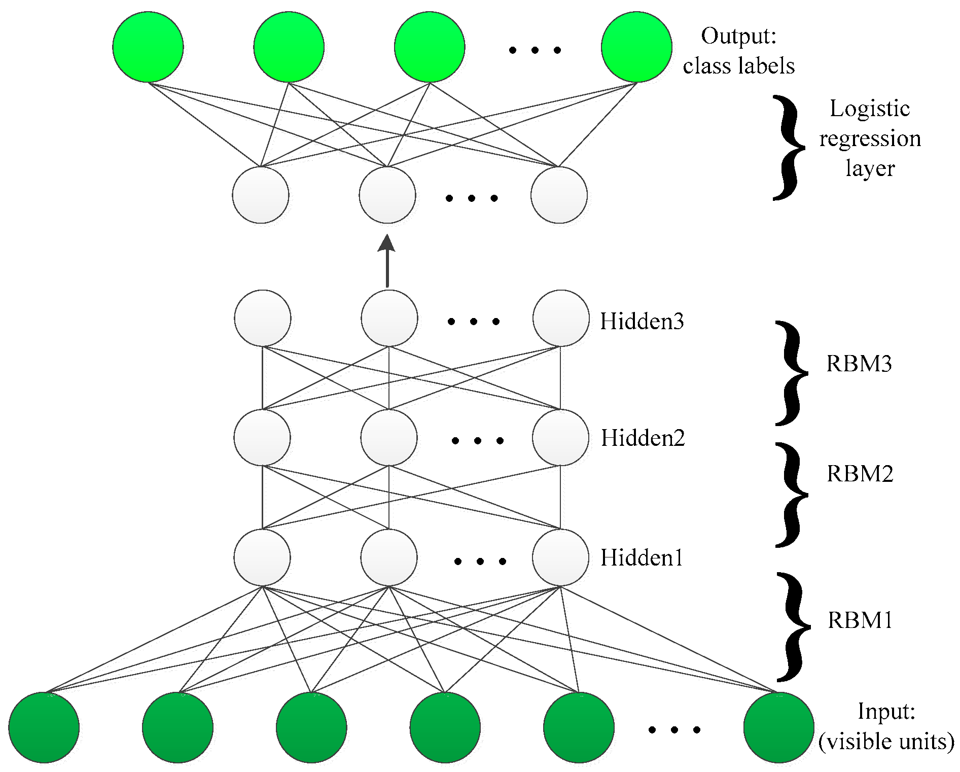
2.2. Deep Belief Learning
3. The Proposed Framework
3.1. Band Grouping and Sample Band Selection
3.2. Texture Feature Enhancement
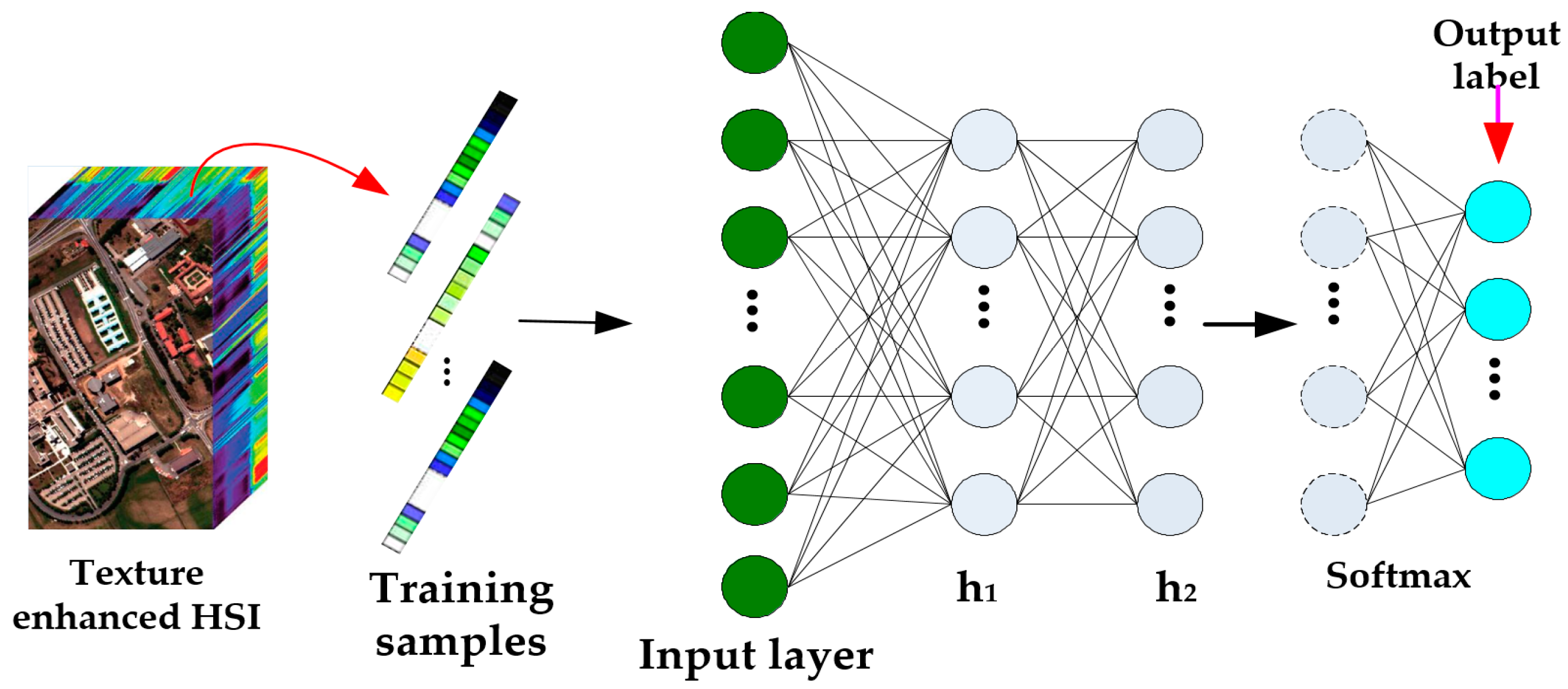
3.3. DBN Classification Model
4. Experiments
4.1. Datasets
4.2. Parameters Tuning and Analysis
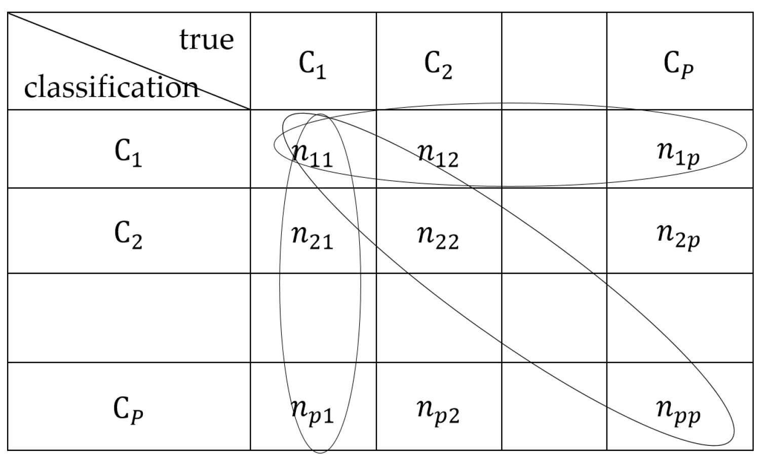
4.3. Evaluation Criteria
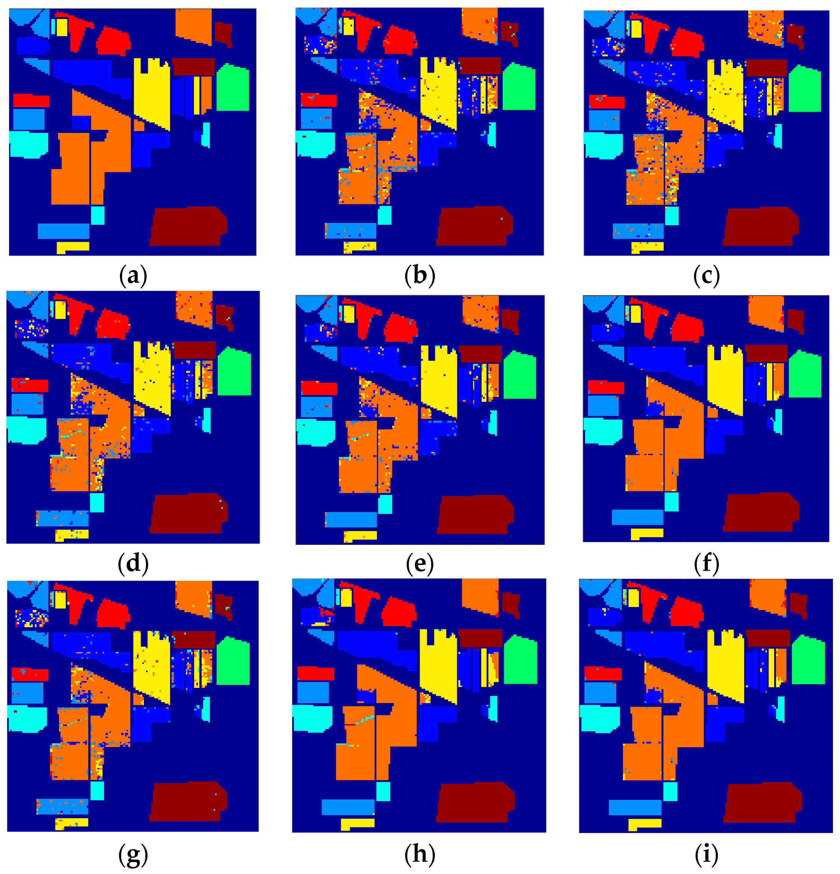
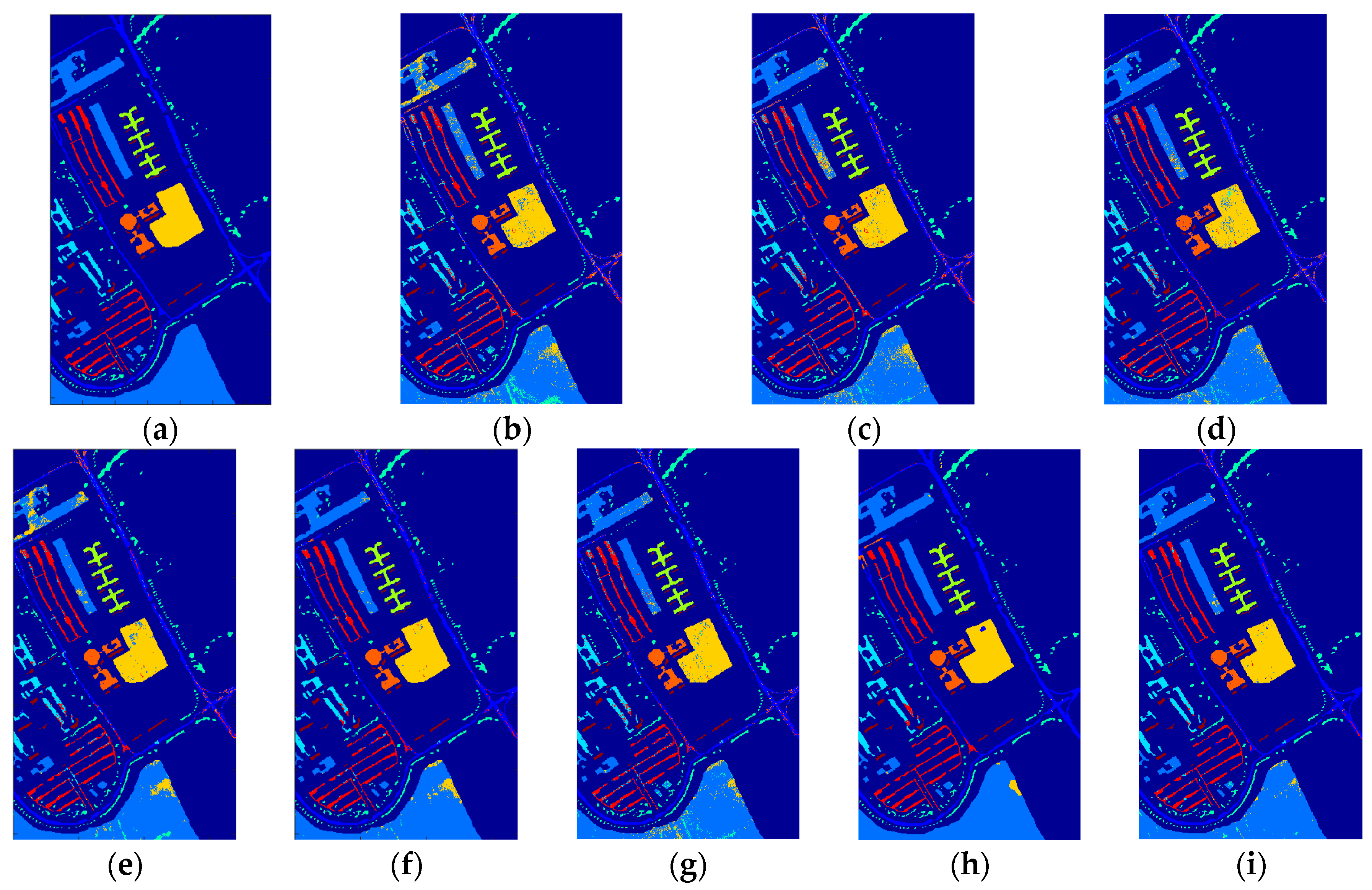
5. Experimental Results and Discussion
5.1. Compared Methods and Band Groups
5.2. Discussion on Effectiveness of the Proposed TFE
5.3. Discussion on Classification Results and Statistical Test
6. Conclusions
Acknowledgments
Author Contributions
Conflicts of Interest
References
- Adão, T.; Hruška, J.; Pádua, L.; Bessa, J.; Peres, E.; Morais, R.; Sousa, J.J. Hyperspectral Imaging: A Review on UAV-Based Sensors, Data Processing and Applications for Agriculture and Forestry. Remote Sens. Agric. Veg. 2017, 9, 1110. [Google Scholar] [CrossRef]
- Yokoya, N.; Chan, J.C.W.; Segl, K. Potential of Resolution-Enhanced Hyperspectral Data for Mineral Mapping Using Simulated EnMAP and Sentinel-2 Images. Remote Sens. 2016, 8, 172. [Google Scholar] [CrossRef]
- Merentitis, A.; Debes, C.; Heremans, R. Ensemble Learning in Hyperspectral Image Classification: Toward Selecting a Favorable Bias-Variance Tradeoff. IEEE J. STARS 2014, 7, 1089–1102. [Google Scholar] [CrossRef]
- He, J.; He, Y.; Zhang, C. Determination and Visualization of Peimine and Peiminine Content in Fritillaria thunbergii Bulbi Treated by Sulfur Fumigation Using Hyperspectral Imaging with Chemometrics. Molecules 2017, 22, 1402. [Google Scholar] [CrossRef] [PubMed]
- Richards, J.A.; Jia, X. Using Suitable Neighbors to Augment the Training Set in Hyperspectral Maximum Likelihood Classification. IEEE Geosci. Remote Sens. Lett. 2008, 5, 774–777. [Google Scholar] [CrossRef]
- Leonenko, G.; Los, S.O.; North, P.R.J. Statistical Distances and Their Applications to Biophysical Parameter Estimation: Information Measures, M-Estimates, and Minimum Contrast Methods. Remote Sens. 2013, 5, 1355–1388. [Google Scholar] [CrossRef]
- Zhang, J.; Mani, I. KNN Approach to Unbalanced Data Distributions: A Case Study Involving Information Extraction. In Proceedings of the ICML 2003 Learning Imbalanced Datasets, Washington, DC, USA, 21–24 August 2003. [Google Scholar]
- Mathew, J.; Luo, M.; Pang, C.K.; Chan, H.L. Kernel-based SMOTE for SVM classification of imbalanced datasets. In Proceedings of the IECON 2015 41st Annual Conference of the IEEE Industrial Electronics Society, Yokohama, Japan, 9–12 November 2015; pp. 001127–001132. [Google Scholar]
- Immitzer, M.; Atzberger, C.; Koukal, T. Tree Species Classification with Random Forest Using Very High Spatial Resolution 8-Band WorldView-2 Satellite Data. Remote Sens. 2012, 4, 2661–2693. [Google Scholar] [CrossRef]
- Dobigeon, N.; Tourneret, J.Y.; Chang, C.I. Semi-Supervised Linear Spectral Unmixing Using a Hierarchical Bayesian Model for Hyperspectral Imagery. IEEE Trans. Signal Process. 2008, 56, 2684–2695. [Google Scholar] [CrossRef]
- Zhang, L.; Wei, W.; Zhang, Y.; Li, F.; Yan, H. Structured sparse BAYESIAN hyperspectral compressive sensing using spectral unmixing. In Proceedings of the 2014 6th Workshop on Hyperspectral Image and Signal Processing: Evolution in Remote Sensing (WHISPERS), Lausanne, Switzerland, 24–27 June 2014. [Google Scholar]
- Yu, H.; Gao, L.; Li, J.; Li, S.S.; Zhang, B.; Benediktsson, J.A. Spectral-Spatial Hyperspectral Image Classification Using Subspace-Based Support Vector Machines and Adaptive Markov Random Fields. Remote Sens. 2016, 8, 355. [Google Scholar] [CrossRef]
- Chen, H.M.; Wang, H.C.; Chai, J.W.; Chen, C.C.C.; Xue, B.; Wang, L.; Yu, C.; Wang, Y.; Song, M.; Chang, C.I. A Hyperspectral Imaging Approach to White Matter Hyperintensities Detection in Brain Magnetic Resonance Images. Remote Sens. 2017, 9, 1174. [Google Scholar] [CrossRef]
- Kayabol, K. Bayesian Gaussian mixture model for spatial-spectral classification of hyperspectral images. In Proceedings of the 2015 23rd European Signal Processing Conference (EUSIPCO), Nice, France, 31 August–4 September 2015; pp. 1805–1809. [Google Scholar]
- Ramo, R.; Chuvieco, E. Developing a Random Forest Algorithm for MODIS Global Burned Area Classification. Remote Sens. 2017, 9, 1193. [Google Scholar] [CrossRef]
- Starck, J.; Elad, M.; Donoho, D. Image decomposition via the combination of sparse representation and a variational approach. IEEE Trans. Image Process. 2005, 14, 1570–1582. [Google Scholar] [CrossRef] [PubMed]
- Wright, J.; Yang, A.Y.; Ganesh, A.; Sastry, S.S.; Ma, Y. Robust face recognition via sparse representation. IEEE Trans. Pattern Anal. Mach. Intell. 2009, 31, 210–226. [Google Scholar] [CrossRef] [PubMed]
- Zhang, L.; Zhou, W.D.; Chang, P.C.; Yan, Z.; Wang, T.; Li, F.Z. Kernel Sparse Representation-Based Classifier. IEEE Trans. Signal Process. 2012, 60, 1684–1695. [Google Scholar] [CrossRef]
- Chen, Y.; Nasrabadi, N.M.; Tran, T.D. Hyperspectral image classification using dictionary-based sparse representation. IEEE Trans. Geosci. Remote Sens. 2011, 49, 3973–3985. [Google Scholar] [CrossRef]
- Chen, Y.; Nasrabadi, N.M.; Tran, T.D. Hyperspectral image classification via kernel sparse representation. IEEE Trans. Geosci. Remote Sens. 2013, 51, 217–231. [Google Scholar] [CrossRef]
- Li, W.; Tramel, E.W.; Prasad, S.; Fowler, J.E. Nearest regularized subspace for hyperspectral classification. IEEE Trans. Geosci. Remote Sens. 2014, 52, 477–489. [Google Scholar] [CrossRef]
- Kang, X.; Li, S.; Benediktsson, J.A. Spectral–Spatial Hyperspectral Image Classification with Edge-Preserving Filtering. IEEE Trans. Geosci. Remote Sens. 2014, 52, 2666–2677. [Google Scholar] [CrossRef]
- Chen, C.; Li, W.; Su, H.; Liu, K. Spectral-Spatial Classification of Hyperspectral Image Based on Kernel Extreme Learning Machine. Remote Sens. 2014, 6, 5795–5814. [Google Scholar] [CrossRef]
- Wang, T.; Zhang, H.; Lin, H.; Fang, C. Textural–Spectral Feature-Based Species Classification of Mangroves in Mai Po Nature Reserve from Worldview-3 Imagery. Remote Sens. 2016, 8, 24. [Google Scholar] [CrossRef]
- Zhong, Y.; Jia, T.; Zhao, J.; Wang, X.; Jin, S. Spatial-Spectral-Emissivity Land-Cover Classification Fusing Visible and Thermal Infrared Hyperspectral Imagery. Remote Sens. 2017, 9, 910. [Google Scholar] [CrossRef]
- Peng, B.; Li, W.; Xie, X.; Du, Q.; Liu, K. Weighted-Fusion-Based Representation Classifiers for Hyperspectral Imagery. Remote Sens. 2015, 7, 14806–14826. [Google Scholar] [CrossRef]
- Fukushima, K. Neocognitron: A hierarchical neural network capable of visual pattern recognition. Neural Netw. 1988, 1, 119–130. [Google Scholar] [CrossRef]
- Ciresan, D.C.; Meier, U.; Masci, J.; Gambardella, L.M.; Schmidhuber, J. Flexible, high performance convolutional neural networks for image classification. In Proceedings of the Joint Conference Artificial Intelligence (IJCAI ’11), Barcelona, Catalonia, Spain, 16–22 July 2011; pp. 1237–1242. [Google Scholar]
- Lee, H.; Kwon, H. Going Deeper with Contextual CNN for Hyperspectral Image Classification. IEEE Trans. Image Process. 2017, 26, 4843–4855. [Google Scholar] [CrossRef] [PubMed]
- Chen, Y.; Jiang, H.; Li, C.; Jia, X.; Ghamisi, P. Deep Feature Extraction and Classification of Hyperspectral Images Based on Convolutional Neural Networks. IEEE Trans. Geosci. Remote Sens. 2016, 54, 6232–6251. [Google Scholar] [CrossRef]
- Chen, Y.; Zhao, X.; Jia, X. Spectral–Spatial Classification of Hyperspectral Data Based on Deep Belief Network. IEEE J. STARS 2015, 8, 2381–2392. [Google Scholar] [CrossRef]
- Özdemir, A.O.B.; Gedik, B.E.; Çetin, C.Y.Y. Hyperspectral classification using stacked autoencoders with deep learning. In Proceedings of the 2014 6th Workshop on Hyperspectral Image and Signal Processing: Evolution in Remote Sensing (WHISPERS), Lausanne, Switzerland, 24–27 June 2014. [Google Scholar]
- Hinton, G.E.; Slakhutdinov, R.R. Reducing the Dimensionality of Data with Neural Networks. Science 2006, 313, 504–507. [Google Scholar] [CrossRef] [PubMed]
- Ohanian, P.P.; Dubes, R.C. Performance evaluation for four classes of textural features. Pattern Recognit. 1992, 25, 819–833. [Google Scholar] [CrossRef]
- Xue, B.; Yu, C.; Wang, Y.; Song, M.; Li, S.; Wang, L. A subpixel target detection approach to hyperspectral image classification. IEEE Trans. Geosci. Remote Sens. 2017, 55, 5093–5114. [Google Scholar] [CrossRef]
- Foody, G.M. Thematic map comparison: Evaluating the statistical significance of differences in classification accuracy. Photogramm. Eng. Remote Sens. 2004, 70, 627–633. [Google Scholar] [CrossRef]


| No. | Feature | Formula |
|---|---|---|
| Energy | ||
| Entropy | ||
| Contrast | ||
| Mean | ||
| Homogeneity |
| No. | Classes | Training | Testing |
|---|---|---|---|
| 1 | Corn-notill | 300 | 1160 |
| 2 | Corn-mintill | 300 | 534 |
| 3 | Grass-pasture | 300 | 197 |
| 4 | Hay-windrowed | 300 | 189 |
| 5 | Soybean-notill | 300 | 668 |
| 6 | Soybean-mintill | 300 | 2168 |
| 7 | Soybean-clean | 300 | 314 |
| 8 | Woods | 300 | 994 |
| Total | 2400 | 6224 |
| No. | Classes | Training | Testing |
|---|---|---|---|
| 1 | Asphalt | 300 | 6331 |
| 2 | Meadows | 300 | 18,349 |
| 3 | Gravel | 300 | 1799 |
| 4 | Trees | 300 | 2764 |
| 5 | Painted metal sheets | 300 | 1045 |
| 6 | Bare Soil | 300 | 4729 |
| 7 | Bitumen | 300 | 1030 |
| 8 | Self-Blocking Bricks | 300 | 3382 |
| 9 | Shadows | 300 | 647 |
| Total | 2700 | 40,076 |
| No. | Classes | Training | Testing |
|---|---|---|---|
| 1 | Brocoli_green_weeds_1 | 300 | 1709 |
| 2 | Brocoli_green_weeds_2 | 300 | 3426 |
| 3 | Fallow | 300 | 1676 |
| 4 | Fallow_rough_plow | 300 | 1094 |
| 5 | Fallow_smooth | 300 | 2378 |
| 6 | Stubble | 300 | 3659 |
| 7 | Celery | 300 | 3279 |
| 8 | Grapes_untrained | 300 | 10,971 |
| 9 | Soil_vinyard_develop | 300 | 5903 |
| 10 | Corn_senesced_green_weeds | 300 | 2978 |
| 11 | Lettuce_romaine_4wk | 300 | 768 |
| 12 | Lettuce_romaine_5wk | 300 | 1627 |
| 13 | Lettuce_romaine_6wk | 300 | 616 |
| 14 | Lettuce_romaine_7wk | 300 | 770 |
| 15 | Vinyard_untrained | 300 | 6968 |
| 16 | Vinyard_vertical_trellis | 300 | 1507 |
| Total | 4800 | 49,329 |
| Datasets | 1 Layer | 2 Layers | 3 Layers | 4 Layers |
|---|---|---|---|---|
| Indian Pines | 0.8919 | 0.8948 | 0.8892 | 0.8432 |
| University of Pavia | 0.9090 | 0.9123 | 0.9065 | 0.8994 |
| Salinas | 0.9123 | 0.9228 | 0.9104 | 0.9064 |
| Class | SVM | RBFNN | O_DBN | SVM_TFE | RBFNN_TFE | CNN | EPF-G-c | Our Proposed |
|---|---|---|---|---|---|---|---|---|
| 1 | 0.8578 | 0.8672 | 0.8562 | 0.9069 | 0.9638 | 0.9107 | 0.9757 | 0.9690 |
| 2 | 0.9251 | 0.9288 | 0.9532 | 0.9625 | 0.9944 | 0.7783 | 0.9736 | 0.9888 |
| 3 | 0.9391 | 0.9543 | 0.9594 | 0.9594 | 0.9949 | 0.8462 | 0.9314 | 0.9594 |
| 4 | 0.9841 | 1 | 0.9947 | 1 | 1 | 0.9793 | 0.9793 | 1 |
| 5 | 0.9162 | 0.9237 | 0.9172 | 0.9506 | 0.9910 | 0.7842 | 0.9268 | 0.9880 |
| 6 | 0.8054 | 0.7975 | 0.8189 | 0.8962 | 0.9553 | 0.9348 | 0.9855 | 0.9613 |
| 7 | 0.9363 | 0.9459 | 0.9490 | 0.9522 | 0.9809 | 0.8442 | 0.9873 | 0.9682 |
| 8 | 0.9940 | 0.9950 | 0.9909 | 1 | 1 | 0.9929 | 0.9881 | 1 |
| OA | 0.8837 | 0.8854 | 0.8948 | 0.9343 | 0.9751 | 0.8983 | 0.9754 | 0.9756 |
| AA | 0.9197 | 0.9265 | 0.9270 | 0.9535 | 0.9850 | 0.8838 | 0.9685 | 0.9793 |
| Kappa | 0.8559 | 0.8582 | 0.8617 | 0.9180 | 0.9688 | 0.8736 | 0.9692 | 0.9694 |
| Class | SVM | RBFNN | O_DBN | SVM_TFE | RBFNN_TFE | CNN | EPF-G-c | Our Proposed |
|---|---|---|---|---|---|---|---|---|
| 1 | 0.8585 | 0.8643 | 0.8563 | 0.9132 | 0.9646 | 0.8440 | 0.9474 | 0.9571 |
| 2 | 0.7577 | 0.7631 | 0.7496 | 0.8877 | 0.9620 | 0.9270 | 0.9606 | 0.9661 |
| 3 | 0.9113 | 0.9353 | 0.8400 | 0.8873 | 0.9849 | 0.9492 | 0.9645 | 0.9692 |
| 4 | 0.9688 | 0.9844 | 0.9495 | 0.9895 | 1 | 1.0000 | 1 | 1 |
| 5 | 0.7917 | 0.7434 | 0.8037 | 0.8675 | 0.9272 | 0.9087 | 0.965 | 0.9396 |
| 6 | 0.9307 | 0.9341 | 0.9417 | 0.9643 | 0.9862 | 0.8538 | 0.9686 | 0.9836 |
| 7 | 0.7861 | 0.8710 | 0.8466 | 0.8617 | 0.9716 | 0.9490 | 0.9936 | 0.9882 |
| 8 | 0.9930 | 0.9940 | 0.9970 | 0.9990 | 1 | 0.9909 | 1 | 1 |
| Precision | 0.8747 | 0.8862 | 0.8731 | 0.9213 | 0.9746 | 0.9278 | 0.9750 | 0.9755 |
| Class | SVM | RBFNN | O_DBN | SVM_TFE | RBFNN_TFE | CNN | EPF-G-c | Our Proposed |
|---|---|---|---|---|---|---|---|---|
| 1 | 0.7466 | 0.7733 | 0.8650 | 0.8534 | 0.9029 | 0.9758 | 0.9579 | 0.9458 |
| 2 | 0.8442 | 0.8980 | 0.9281 | 0.9058 | 0.9601 | 0.9832 | 0.9993 | 0.9728 |
| 3 | 0.8533 | 0.8377 | 0.8410 | 0.8922 | 0.9305 | 0.7795 | 0.9511 | 0.9550 |
| 4 | 0.9801 | 0.9602 | 0.9765 | 0.9772 | 0.9787 | 0.9096 | 0.9677 | 0.9881 |
| 5 | 0.9990 | 0.9990 | 0.9990 | 0.9981 | 0.9971 | 0.9830 | 0.9372 | 0.9990 |
| 6 | 0.9108 | 0.9492 | 0.9125 | 0.9558 | 0.9903 | 0.8153 | 0.9263 | 0.9873 |
| 7 | 0.9456 | 0.9583 | 0.8990 | 0.9544 | 0.9932 | 0.6680 | 0.9885 | 0.9893 |
| 8 | 0.8430 | 0.8628 | 0.8613 | 0.9101 | 0.9571 | 0.8562 | 0.9421 | 0.9438 |
| 9 | 1 | 1 | 0.9985 | 1 | 1 | 0.9985 | 0.9895 | 1.0000 |
| OA | 0.8555 | 0.8888 | 0.9123 | 0.9133 | 0.9568 | 0.9211 | 0.9671 | 0.9696 |
| AA | 0.9025 | 0.9154 | 0.9201 | 0.9385 | 0.9678 | 0.8855 | 0.9622 | 0.9757 |
| Kappa | 0.8103 | 0.8525 | 0.8824 | 0.8845 | 0.9418 | 0.8943 | 0.9590 | 0.9590 |
| Class | SVM | RBFNN | O_DBN | SVM_TFE | RBFNN_TFE | CNN | EPF-G-c | Our Proposed |
|---|---|---|---|---|---|---|---|---|
| 1 | 0.9795 | 0.9798 | 0.9675 | 0.9836 | 0.9877 | 0.8531 | 0.9822 | 0.9837 |
| 2 | 0.9720 | 0.9841 | 0.9763 | 0.9869 | 0.9980 | 0.9341 | 0.9756 | 0.9978 |
| 3 | 0.6657 | 0.6905 | 0.7568 | 0.7803 | 0.8876 | 0.8766 | 0.9711 | 0.9261 |
| 4 | 0.7657 | 0.8906 | 0.8207 | 0.9122 | 0.9808 | 0.9678 | 0.9642 | 0.9437 |
| 5 | 0.9831 | 0.9981 | 0.9849 | 0.9943 | 1 | 0.9981 | 0.9900 | 0.9877 |
| 6 | 0.6714 | 0.7388 | 0.7735 | 0.7456 | 0.8639 | 0.9484 | 0.9450 | 0.9189 |
| 7 | 0.5084 | 0.5583 | 0.6515 | 0.7567 | 0.8575 | 0.9592 | 0.9157 | 0.9586 |
| 8 | 0.8312 | 0.8028 | 0.8645 | 0.8394 | 0.8772 | 0.8752 | 0.9864 | 0.9117 |
| 9 | 1 | 1 | 0.9985 | 0.9985 | 1 | 0.9985 | 0.8779 | 0.9969 |
| Precision | 0.8197 | 0.8492 | 0.8660 | 0.8886 | 0.9392 | 0.9345 | 0.9565 | 0.9583 |
| Class | SVM | RBFNN | O_DBN | SVM_TFE | RBFNN_TFE | CNN | EPF-G-c | Our Proposed |
|---|---|---|---|---|---|---|---|---|
| 1 | 0.9965 | 0.9971 | 0.9947 | 0.9982 | 0.9988 | 1.0000 | 1.0000 | 0.9947 |
| 2 | 0.9947 | 0.9947 | 1 | 0.9956 | 0.9950 | 0.9933 | 0.9994 | 0.9962 |
| 3 | 0.9976 | 0.9988 | 0.9976 | 0.9976 | 0.9982 | 0.9589 | 0.9994 | 0.9976 |
| 4 | 0.9963 | 0.9963 | 0.9963 | 0.9954 | 0.9954 | 0.9838 | 0.9973 | 0.9973 |
| 5 | 0.9886 | 0.9849 | 0.9811 | 0.9874 | 0.9899 | 0.9898 | 0.9992 | 0.9853 |
| 6 | 0.9981 | 0.9986 | 0.9978 | 0.9981 | 0.9981 | 0.9995 | 0.9984 | 0.9973 |
| 7 | 0.9970 | 0.9963 | 0.9957 | 0.9960 | 0.9966 | 0.9988 | 0.9989 | 0.9963 |
| 8 | 0.8606 | 0.8567 | 0.8315 | 0.8761 | 0.8893 | 0.8379 | 0.8690 | 0.9085 |
| 9 | 0.9934 | 0.9985 | 0.9939 | 0.9942 | 0.9966 | 0.9896 | 0.9911 | 0.9949 |
| 10 | 0.9661 | 0.9758 | 0.9426 | 0.9698 | 0.9775 | 0.8848 | 0.9715 | 0.9614 |
| 11 | 0.9987 | 0.9961 | 0.9961 | 0.9987 | 0.9987 | 0.8919 | 1 | 1 |
| 12 | 0.9994 | 1 | 1 | 0.9994 | 1 | 0.9685 | 0.9992 | 0.9994 |
| 13 | 0.9968 | 0.9951 | 0.9984 | 0.9951 | 0.9951 | 0.9534 | 0.9987 | 0.9968 |
| 14 | 0.9792 | 0.9857 | 0.9948 | 0.9857 | 0.9805 | 0.9159 | 0.9978 | 0.9948 |
| 15 | 0.6972 | 0.7336 | 0.7646 | 0.7941 | 0.7916 | 0.7673 | 0.8856 | 0.9127 |
| 16 | 0.9920 | 0.9900 | 0.9854 | 0.9920 | 0.9914 | 0.9695 | 1 | 0.9887 |
| OA | 0.9212 | 0.9266 | 0.9228 | 0.9387 | 0.9421 | 0.9155 | 0.9543 | 0.9622 |
| AA | 0.9658 | 0.9687 | 0.9669 | 0.9733 | 0.9746 | 0.9439 | 0.9816 | 0.9826 |
| Kappa | 0.9114 | 0.9175 | 0.9133 | 0.9312 | 0.9350 | 0.9051 | 0.9486 | 0.9575 |
| Class | SVM | RBFNN | O_DBN | SVM_TFE | RBFNN_TFE | CNN | EPF-G-c | Our Proposed |
|---|---|---|---|---|---|---|---|---|
| 1 | 0.9988 | 0.9994 | 0.9971 | 0.9994 | 1 | 0.9801 | 1 | 1 |
| 2 | 0.9985 | 0.9985 | 0.9980 | 0.9994 | 0.9994 | 0.9947 | 0.9995 | 0.9991 |
| 3 | 0.9744 | 0.9721 | 0.9489 | 0.9830 | 0.9824 | 0.9976 | 0.9782 | 0.9682 |
| 4 | 0.9909 | 0.9864 | 0.9847 | 0.9918 | 0.9900 | 0.9973 | 0.9991 | 0.9900 |
| 5 | 0.9941 | 0.9970 | 0.9978 | 0.9920 | 0.9895 | 0.9315 | 0.9987 | 0.9924 |
| 6 | 0.9995 | 0.9997 | 0.9884 | 0.9992 | 0.9995 | 0.9978 | 0.9997 | 0.9940 |
| 7 | 0.9966 | 1 | 1 | 0.9951 | 1 | 0.9957 | 0.9991 | 0.9973 |
| 8 | 0.8209 | 0.8372 | 0.8592 | 0.8729 | 0.8726 | 0.8952 | 0.9162 | 0.9415 |
| 9 | 0.9956 | 0.9916 | 0.9898 | 0.9931 | 0.9927 | 0.9810 | 0.9475 | 0.9926 |
| 10 | 0.9517 | 0.9735 | 0.8699 | 0.9534 | 0.9674 | 0.9325 | 0.9627 | 0.9487 |
| 11 | 0.9808 | 0.9922 | 0.8242 | 0.9935 | 0.9948 | 0.9831 | 0.9994 | 0.9785 |
| 12 | 0.9909 | 0.9897 | 0.9748 | 0.9933 | 0.9921 | 1.0000 | 0.9987 | 0.9933 |
| 13 | 0.9777 | 0.9919 | 0.9935 | 0.9871 | 0.9839 | 0.9968 | 0.9920 | 0.9731 |
| 14 | 0.8737 | 0.9245 | 0.8235 | 0.9256 | 0.8945 | 0.9506 | 0.9359 | 0.8899 |
| 15 | 0.7803 | 0.7747 | 0.7344 | 0.8187 | 0.8341 | 0.5128 | 0.7777 | 0.8559 |
| 16 | 0.9701 | 0.9920 | 0.9861 | 0.9658 | 0.9953 | 0.9854 | 0.9946 | 0.9900 |
| Precision | 0.9559 | 0.9638 | 0.9356 | 0.9665 | 0.9680 | 0.9458 | 0.9687 | 0.9690 |
| Algorithms | Indian Pines | Pavia University | Salinas |
|---|---|---|---|
| SVM | 31.16/Yes | 68.33/Yes | 41.19/Yes |
| RBFNN | 31.34/Yes | 69.27/Yes | 41.39/Yes |
| O_DBN | 2.78/Yes | 3.74/Yes | 3.32/Yes |
| SVM_TFE | 31.95/Yes | 73.29/Yes | 41.21/Yes |
| RBFNN_TFE | 32.82/Yes | 74.84/Yes | 42.49/Yes |
| CNN | 3.50/Yes | 3.00/Yes | 4.49/Yes |
| EPF_G_c | 32.16/Yes | 75.13/Yes | 41.21/Yes |
© 2018 by the authors. Licensee MDPI, Basel, Switzerland. This article is an open access article distributed under the terms and conditions of the Creative Commons Attribution (CC BY) license (http://creativecommons.org/licenses/by/4.0/).
Share and Cite
Li, J.; Xi, B.; Li, Y.; Du, Q.; Wang, K. Hyperspectral Classification Based on Texture Feature Enhancement and Deep Belief Networks. Remote Sens. 2018, 10, 396. https://doi.org/10.3390/rs10030396
Li J, Xi B, Li Y, Du Q, Wang K. Hyperspectral Classification Based on Texture Feature Enhancement and Deep Belief Networks. Remote Sensing. 2018; 10(3):396. https://doi.org/10.3390/rs10030396
Chicago/Turabian StyleLi, Jiaojiao, Bobo Xi, Yunsong Li, Qian Du, and Keyan Wang. 2018. "Hyperspectral Classification Based on Texture Feature Enhancement and Deep Belief Networks" Remote Sensing 10, no. 3: 396. https://doi.org/10.3390/rs10030396
APA StyleLi, J., Xi, B., Li, Y., Du, Q., & Wang, K. (2018). Hyperspectral Classification Based on Texture Feature Enhancement and Deep Belief Networks. Remote Sensing, 10(3), 396. https://doi.org/10.3390/rs10030396