Abstract
The Cushing Hub in Oklahoma, one of the largest oil storage facilities in the world, is federally designated as critical national infrastructure. In 2014, the formerly aseismic city of Cushing experienced a Mw 4.0 and 4.3 induced earthquake sequence due to wastewater injection. Since then, an M4+ earthquake sequence has occurred annually (October 2014, September 2015, November 2016). Thus far, damage to critical infrastructure has been minimal; however, a larger earthquake could pose significant risk to the Cushing Hub. In addition to inducing earthquakes, wastewater injection also threatens the Cushing Hub through gradual surface uplift. To characterize the impact of wastewater injection on critical infrastructure, we use Differential Interferometric Synthetic Aperture Radar (DInSAR), a satellite radar technique, to observe ground surface displacement in Cushing before and during the induced Mw 5.0 event. Here, we process interferograms of Single Look Complex (SLC) radar data from the European Space Agency (ESA) Sentinel-1A satellite. The preearthquake interferograms are used to create a time series of cumulative surface displacement, while the coseismic interferograms are used to invert for earthquake source characteristics. The time series of surface displacement reveals 4–5.5 cm of uplift across Cushing over 17 months. The coseismic interferogram inversion suggests that the 2016 Mw 5.0 earthquake is shallower than estimated from seismic inversions alone. This shallower source depth should be taken into account in future hazard assessments for regional infrastructure. In addition, monitoring of surface deformation near wastewater injection wells can be used to characterize the subsurface dynamics and implement measures to mitigate damage to critical installations.
1. Introduction
Cushing, Oklahoma, the “pipeline crossroads of the world,” is home to the largest crude oil storage facility in the United States and the Keystone pipeline. Wastewater injection threatens this critical national energy infrastructure through both large, instantaneous ground acceleration from induced seismicity and through smaller, incremental, longer term movement from ground surface deformation [1].
Prior to 2009, seismicity in Oklahoma was concentrated along the Meers fault zone, southwest of the recently reactivated Nemaha and Wilzetta fault zones [2]. Since seismicity initiated in Cushing in 2014, three earthquake sequences have ruptured two fault zones (Figure 1). The October 2014 sequence, just south of Cushing, consisted of two moderate sized, shallow earthquakes, a Mw 4.0 on 7 October followed by a Mw 4.3 on 10 October [3]. The aftershock alignment revealed the reactivation of the unmapped Cushing fault, a 5 km long, N80W striking, left-lateral, strike-slip conjugate fault within the Wilzetta–Whitetail fault zone [3].
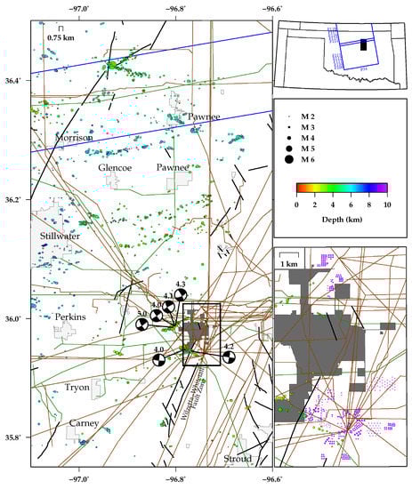
Figure 1.
Map of geocoded area of interest showing relocated seismicity from May 2013 to November 2016 [5] (scaled colored circles), focal mechanisms for major Cushing earthquakes, faults [15] (black lines), municipal boundaries (light gray polygons), Cushing city boundary (dark gray polygon), gaslines (green lines), oil pipelines (brown lines), and outline of Sentinel-1A footprint (blue rectangle). The top right figure shows the outline of Sentinel-1A footprint (blue rectangle) and the location of the geocoded area (filled black rectangle). The bottom right figure is an inset with a zoomed in view of Cushing showing critical infrastructure such as gaslines (green lines), oil pipelines (brown lines), and storage tanks (purple dots).
In 2015, the seismicity shifted to the west of Cushing to an unmapped northwest striking, right-lateral, strike-slip fault. The 2015 sequence consisted of an M4.1 on 18 September, an M4.0 on 25 September, and an M4.3 on 10 October [4,5]. The November 2016 sequence occurred on the southern end of the same unmapped fault. This third sequence consisted of 48 earthquakes of M3 or greater, most of which were foreshocks, while only six were aftershocks [4]. The Mw 5.0 mainshock on 7 November 2016 was characterized as a right-lateral, strike-slip event. The aftershock pattern revealed that the mainshock ruptured around the rupture planes of 2015 M4 earthquakes [6]. The 2015 and 2016 sequences occurred in an area where static stress change from the 2014 sequence is negligible [3].
The 2016 mainshock caused significant damage to buildings and infrastructure in downtown Cushing [7]. Even though the damage to oil and gas infrastructure was minimal due to its location, the smaller October 2014 earthquake sequence reactivated the Cushing fault which underlies this critical infrastructure. The increase in static stress from the 2014 sequence suggests the Cushing fault can host earthquakes as large as the 2011 Mw 5.6 Prague earthquake [3].
Although it is well-established that large-scale wastewater disposal in the Arbuckle formation is linked to the recent rise in seismicity in Oklahoma [4,8,9,10,11], few studies in Oklahoma have shown surface deformation resulting from induced seismicity [12] or from wastewater injection [13] or both [14]. In our two-part study, we observe both the surface deformation leading up to the November 2016 Mw 5.0 earthquake and its coseismic signal using a satellite radar technique known as Differential Interferometric Synthetic Aperture Radar (DInSAR). In the first half, we perform a spatiotemporal correlation analysis of DInSAR derived surface deformation, wastewater injection, and seismicity in Cushing, OK. In the second half of the analysis, we invert for the source of the November 2016 event using DInSAR coseismic images, we classify photos of structural damage for the event, and compare their spatial signature.
2. Data
2.1. Synthetic Aperture Radar Data
To measure the surface displacement before and during the 2016 earthquake sequence, we process 32 European Satellite Agency (ESA) Copernicus Sentinel-1A (S1A) Synthetic Aperture Radar (SAR) Single Look Complex (SLC) images from the Alaska Satellite Facility (ASF). The SAR images spanning the Cushing area correspond to ascending relative orbit 34, frames 109–113 (north) and 114–118 (south), swaths 2 and 3 (Figure 1). Table 1 lists the acquisition dates used for this study. The dates are separated by a dashed horizontal line, with preearthquake dates listed above and postearthquake dates listed below the horizontal line. We multilook the data, applying 12 looks in range and two looks in azimuth. For time series pairs, we apply a temporal baseline threshold of 12 days to minimize decorrelation due to vegetation (Table 2). We make an exception for a few pairs by increasing the temporal baseline up to 60 days to complete the network connectivity. For the source inversion, we pair images with a temporal baseline threshold of 36 days (Figure 2).

Table 1.
Sentinel-1A acquisition dates used in the study.
Table 2.
Perpendicular and temporal baselines for S1A time series interferograms. Bperp = Perpendicular baseline. T = Temporal baseline.
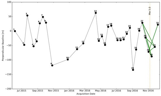
Figure 2.
Perpendicular baseline plot for pairs (solid lines) showing acquisition dates (circles) and 2016 Mw 5.0 Cushing earthquake (vertical gold dashed line). Gray lines are the preearthquake pairs used in time series analysis while green lines are coseismic pairs used for source inversion.
2.2. Damage Data
We assess the damage caused by the Mw 5.0 event by analyzing damage data collected by the Earthquake Engineering Research Institute (EERI) reconnaissance team following the 7 November 2016 earthquake. The EERI Clearinghouse database [16] consists of over 1400 photos of damage for the 2016 Pawnee and Cushing earthquakes (Figure 3). Each of these photos contains information including the latitude and longitude, and a description of damage.
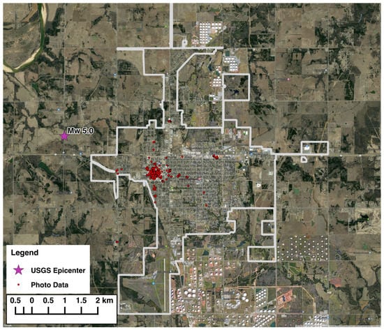
Figure 3.
Damage data (red circles) for the city of Cushing (gray outline) and the United States Geological Survey (USGS) Mw 5.0 epicenter (magenta star). Each red circle represents a collected photo of building and infrastructure damage. A single building or infrastructure can have multiple photos of damage associated (multiple data points).
3. Methods
3.1. InSAR Processing
We perform interferometry on the SAR data using the Jet Propulsion Laboratory (JPL)/Caltech Interferometric SAR Scientific Computing Environment (ISCE) software [17]. The interferograms are corrected for topography using a 10-meter United States Geological Survey (USGS) National Elevation Dataset (NED) Digital Elevation Model (DEM). A Gaussian filter of strength 0.6 is applied to facilitate the unwrapping process. Interferograms are unwrapped using the Statistical-Cost, Network-Flow Algorithm for Phase Unwrapping (SNAPHU) algorithm [18,19,20]
The time series of the cumulative surface displacement in the satellite line-of-sight (LOS) for the preseismic interferograms is constructed using the Generic InSAR Analysis Toolbox (GIAnT) software [21]. In GIAnT, we mask pixels whose phase coherence is less than 0.35, we correct for the atmospheric phase delay using the European Centre for Medium-Range Weather Forecasts (ECMWF) global atmospheric model, and we deramp the interferograms. After applying the corrections, we generate the time series using the New Small BAseline Subset (NSBAS) algorithm [22]. We select a reference region in the town of Carney, southwest of Cushing. This region was selected to ensure coherence over the time series.
3.2. Macroseismic Field
The EERI reconnaissance team specified a damage level from light to severe for structural, non-structural, and foundation damage for each photo based on post-earthquake site observations [7]. We assign a Modified Mercalli Intensity (MMI) to each set of photos and damage description representing a single building or site [23]. This process was based on matching qualitative descriptions of the MMI scale to the damage descriptions, similar to the technique used by the USGS to quantify damage from Did You Feel It? responses (Table 3) [24,25]. The MMI intensity that matched the observed damage then was assigned to that site. In the event that the observations and descriptions fell between two intensity levels, the higher intensity level was selected to avoid underestimating damage.
Table 3.
Modified Mercalli Intensity (MMI) classification with damage descriptions for the built and natural environments. Modified from Wald and Dewey [25,26].
4. Results
4.1. Surface Displacement Time Series
The surface displacement time series spans 5 June 2015 to 2 November 2016, ending five days before the Mw 5.0 earthquake. The cumulative displacement time series image reveals a broad region of 4 to 6 cm of uplift across the city of Cushing (Figure 4) over 17 months. The broad deformation signal does not correlate with topography nor streams, rivers, or other waterbodies. These waterbodies, which are common sources of noise, do correlate with areas of decoherence (Figure 5). Other broad regions of uplift are also observed in the cities of Stillwater and Perkins. We extract time series for pixels within two regions of interest, the Mw 5.0 earthquake (Figure 6) and downtown Cushing (Figure 7). We compare the displacement time series to seismicity using the Schoenball and Ellsworth [5] waveform-relocated earthquake catalog from May 2013 to November 2016, with a magnitude of completeness of 2.6. Note that the October 2014 Mw 4.3 earthquake featured in earlier figures was downgraded to a Mw 4.2 in the relocated earthquake catalog. Figures, henceforth, will reflect the downgraded magnitude. In addition to seismicity, we also compare the displacement data to monthly injection rates of of class II (oil and gas-related) Underground Injection Control (UIC) wells from the Oklahoma Corporation Commission (OCC) [27]. Wells are split into two types, type 2R for Enhanced Oil Recovery and type 2D for Salt-Water Disposal (SWD). Any well injecting above 300,000 bbl/month is classified as a high-rate injection well. A summary of the UIC wells within 6 km of our regions of interest are presented in Table 4 and Table 5. Wells that have injected or are currently injecting into the Arbuckle have an additional column of information, injection period, where the table lists the time period that the well was injecting into the Arbuckle before the well was plugged and recompleted into a shallower formation, typically the Wilcox formation.
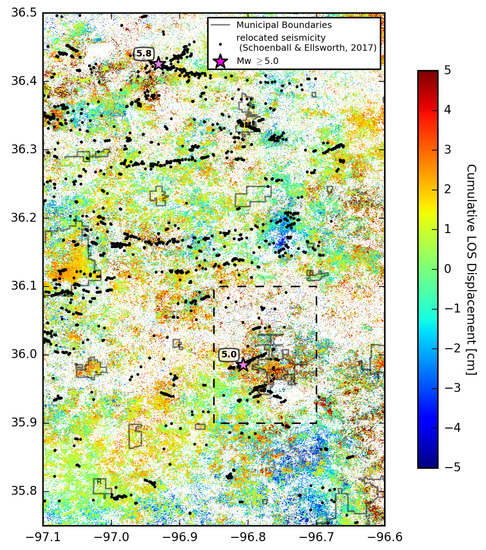
Figure 4.
Cumulative displacement image for geocoded area of interest overlaid with relocated seismicity [5] (black dots), relocated earthquakes > Mw 5.0 (magenta stars), outline of municipalities (gray polygons), reference region (R), and inset location for Figure 5 (dashed rectangle).
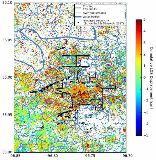
Figure 5.
Cumulative displacement image for Cushing overlaid with rivers and streams (blue lines), waterbodies (blue polygons), relocated seismicity [5] (black dots), relocated earthquakes > Mw 5.0 (magenta stars), and outline of Cushing (black polygon). Pixels not satisfying a coherence threshold of 0.35 have been masked and are colored white.
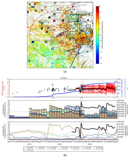
Figure 6.
Cumulative displacement image for selected region near the Mw 5.0 earthquake. (a) cumulative displacement image for selected region (purple polygon). Also overlaid are injection wells (black squares), faults [15], and relocated seismicity [5] (black dots). Relocated M4+ earthquakes (magenta stars) and wells within 6 km of polygon (dashed line) are also plotted and labeled. (b) all three plots feature the average LOS displacement time series for the polygon (black line) and dates of M4+ earthquakes within 6 km (gold vertical dashed lines). Top: LOS displacement time series for each of the pixels within the polygon (transparent red lines), cumulative number of earthquakes within 6 km (blue line), and earthquake magnitudes (light blue circles). Middle: Total monthly injection rate for the 15 injection wells within 6 km of the polygon. Bottom: Individual well monthly injection rates for the 15 wells within 6 km of the polygon.
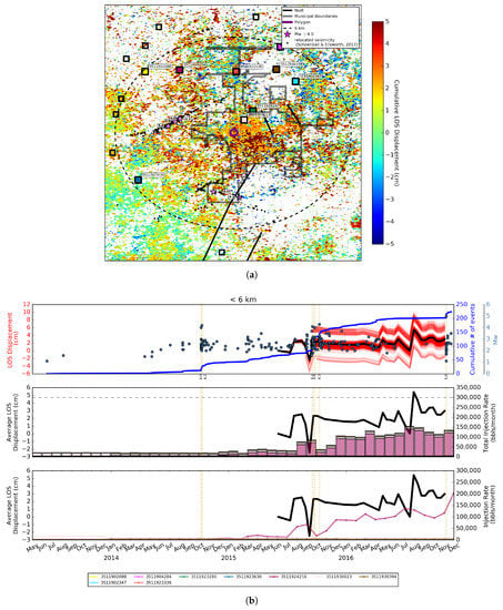
Figure 7.
Cumulative displacement image for selected region in downtown Cushing. (a) cumulative displacement image for selected region (purple polygon). Also overlaid are injection wells (black squares), faults [15], outline of Cushing (gray polygon), and relocated seismicity [5] (black dots). Relocated M4+ earthquakes (magenta stars) and wells within 6 km of polygon (dashed line) are also plotted and labeled. (b) all three plots feature the average LOS displacement time series for the polygon (black line) and dates of M4+ earthquakes within 6 km (gold vertical dashed lines). Top: LOS displacement time series for each of the pixels within the polygon (transparent red lines), cumulative number of earthquakes within 6 km (blue line), and earthquake magnitudes (light blue circles). Middle: Total monthly injection rate for the nine injection wells within 6 km of the polygon. Bottom: Individual well monthly injection rates for the nine wells within 6 km of the polygon.
Table 4.
Class II Underground Injection Control (UIC) wells within 6 km of Mw 5.0 earthquake. * = High-rate injection well. 2R = Enhanced Oil Recovery well. 2D = Salt-Water Disposal well.
Table 5.
Class II Underground Injection Control (UIC) wells within 6 km of downtown Cushing. 2R = Enhanced Oil Recovery well. D = Salt-Water Disposal well.
The cumulative displacement image for the Mw 5.0 earthquake region (Figure 6) shows steady uplift, reaching a maximum of 4.5 cm during the 2015 earthquake sequence. Following the 2015 events, the ground subsides but begins to uplift again almost reaching 4 cm of uplift in the summer of 2016. Although there is no immediate response of ground displacement to injection, there is an increase in displacement during the 2015 earthquake sequence. There was approximately 0.5 cm of uplift that occurred before the Mw 5.0 event. There are 15 UIC wells within 6 km of the Mw 5.0 earthquake (Table 4). All but one well, 2R well API:3511923625, are 2D injection. 2D well API:3511923843, the only high-rate injection well, was high-rate in 2014, just two months before the first Cushing earthquake sequence of 2014.
For downtown Cushing, Figure 7 also shows steady uplift over time with a maximum displacement of 5.5 cm. The temporal signature of the displacement is strikingly similar to the signal for the Mw 5.0 earthquake region. The time series differ in the amplitude of displacement during the 2015 earthquakes and during the summer before the 2016 earthquake. During the 2015 earthquakes, the Mw 5.0 earthquake region, which is near the 2015 events, uplifts 2 cm more than downtown Cushing. Conversely, downtown Cushing experiences 2 cm of uplift more than the Mw 5.0 earthquake region a few months before the Mw 5.0 earthquake. There are nine low-rate UIC wells within 6 km of downtown Cushing, all but one is 2D (Table 5). Six of the nine wells are within 6 km of the Mw 5.0 earthquake region. Unlike the area near the Mw 5.0 earthquake, none of the wells within 6 km of downtown Cushing are injecting into the Arbuckle formation. Thus, the column, “Injection Period,” is omitted from Table 5.
4.2. Source Characterization
We construct six deramped coseismic interferograms (Figure 8) (Table 6). Interferograms 1 to 3 are the least saturated by an atmospheric signal. Interferogram 4, with a 5-day preseismic signal and a 7-day postseismic signal, best represents the earthquake deformation; however, it is heavily saturated by an atmospheric signal. We attribute the atmospheric signal to acquisition date 2 November 2016 due its presence in interferograms 4 through 6. Despite the atmospheric signal, we can see more than 1.6 cm of LOS displacement in opposite directions on both sides of the fault.
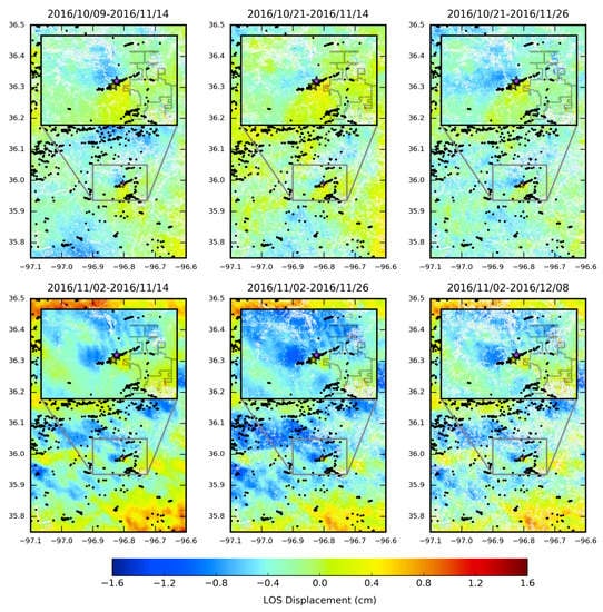
Figure 8.
Deramped, masked coseismic interferograms overlaid with relocated seismicity [5] (black dots), relocated Mw 5.0 epicenter [5] (orange-red star), and USGS epicenter for Mw 5.0 earthquake (magenta star).
Table 6.
S1A coseismic interferograms. Bperp = Perpendicular baseline. T = Temporal baseline.
We average the six coseismic interferograms to increase the signal-to-noise ratio. Using the Pyrocko Kite software [28], we forward model LOS displacement by defining the event as a double-couple point source. We apply a genetic algorithm inversion scheme based on Covariance Matrix Adaptation (CMA-ES) for minimization between our observations and model in a least square sense (L2 norm). We perform 300 evaluations using the USGS National Earthquake Information Center (NEIC) parameters as a priori values. We list our best fit parameters and the the USGS NEIC parameters in Table 7. Our best fit parameters result in an underestimation of displacement (Figure 9), especially on the eastern side of the fault, suggesting the earthquake fault has a smaller dip, and thus has a greater oblique component than our almost purely strike-slip fault model. Forward modeling the USGS NEIC parameters results in an even greater underestimation of displacement on both sides of the fault, suggesting that the earthquake source is shallower than their estimated of 4.4 km (Figure 10).
Table 7.
Inversion parameters.
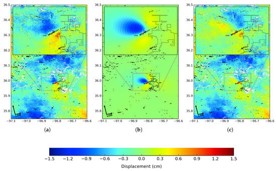
Figure 9.
Best fit forward model comparison to observed LOS displacement. Also plotted is relocated seismicity [5] (black dots), relocated Mw 5.0 epicenter [5] (orange-red star), USGS Mw 5.0 epicenter (magenta star), and the overlapping best-fit Mw 5.0 epicenter (purple star). (a) Observed LOS displacement. (b) Modeled LOS displacement. (c) Residual LOS displacement.
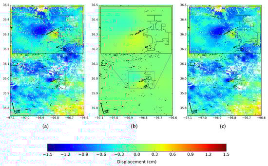
Figure 10.
Forward modeling of 2016 Mw 5.0 earthquake using USGS source parameters. Also plotted is relocated seismicity [5] (black dots), relocated Mw 5.0 epicenter [5] (orange-red star), USGS Mw 5.0 epicenter (magenta star), and the overlapping best-fit Mw 5.0 epicenter (purple star). (a) Observed LOS displacement. (b) Modeled LOS displacement. (c) Residual LOS displacement.
4.3. Damage Assessment
Earthquakes cause building and infrastructure damage through both dynamic shaking and permanent vertical or horizontal displacements of the ground surface. For large earthquakes, obvious manifestations of ground deformation effects include surface fault rupture, large lateral or vertical ground displacements associated with liquefaction, sand boils, landslides, and linear fissures, tilting or racking of homes, and foundation damage [29]. Indicators of more subtle impacts of ground deformation might include utility line breaks, damage to streets, curbs, sidewalks, plumbing, pipe bursts, and foundation cracks. Some examples of damage from ground acceleration are cracks in walls, spalling of exterior facade, permanent drift, and foundation damage. To assess damage from the 2016 Mw 5.0 Cushing earthquake, we remove duplicate data entries for the same damage site representing multiple photos of varying instances of damage. Thus, each point represents a unique damage site where a photo was taken (Figure 11). The selected photos [7] of damage at American Legion, North Route 18 water main, Lion’s Club, and Cimarron Tower from the 2016 Mw 5.0 earthquake, attest to the maximum MMI VII intensity (Figure 12). For comparison with the modeled surface displacement, we select sites with damage indicators like pipe bursts, vertical offsets, and drops in elevation to indicate damage potentially caused or exacerbated by ground deformation (Table 8). Using the preferred parameters, we model the vertical and horizontal components of the surface displacement field (Figure 13) and compare it to the ground failure damage sites. Sites 2 and 3, in the outskirts of town, occur in an area of either high vertical or horizontal displacement. The damage within downtown Cushing at sites 1,4, and 5 can potentially be attributed to a combination of differential settlement and ground acceleration. From Figure 13, we can see the majority of building damage from the earthquake is located in the Central Business District of downtown Cushing, OK. The buildings in this area were constructed between approximately 1910–1940 and are predominantly unreinforced masonry construction with wood framing. When the buildings were constructed, they were not designed to resist wind or seismic forces and thus the buildings may not have complete vertical load paths, or seismic detailing [7]. It is possible that some of the homes in more deformed regions have less damage because the buildings were constructed at a later date or because accelerations were locally lower there. Additionally, the varying geologic conditions between sites, including soil properties, have an impact on the intensity of dynamic shaking, which directly impacts the damage observed. There is a lack of strong motion instrumentation to quantify the differences in dynamic shaking intensity between sites [30].
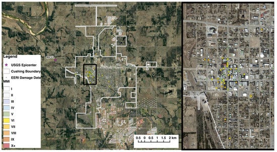
Figure 11.
Google satellite imagery overlaid with Modified Mercalli Intensity (MMI) classified Earthquake Engineering Research Institute (EERI) damage data for the 2016 Cushing earthquake and outline of Cushing (gray polygon).
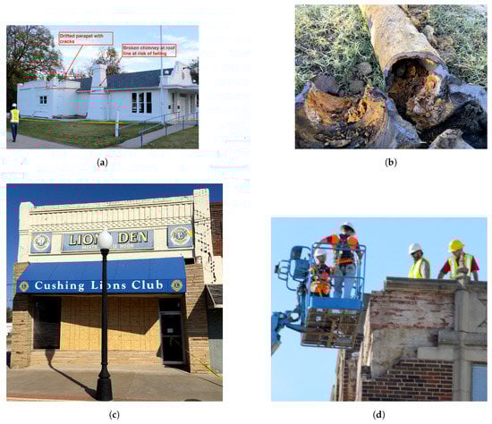
Figure 12.
Examples of characteristic of MMI VII damage from the 2016 Mw 5.0 Cushing earthquake. (a) Damage to the unreinforced masonry American Legion building in Cushing, showing a drifted parapet and chimney broken at roof line and at risk of falling. Although not shown, the back wall fell out. (b) Damage to a water main at North Route 18 showing complete pipe burst potentially due to permanent horizontal and vertical ground deformations. (c) Damage to the unreinforced masonry Lion’s Den in Cushing, showing severe racking at approximately 3 degrees, and separation from the adjacent building. The building collapsed completely a short time after the earthquake. (d) Damage to the Cimarron Tower in Cushing, showing spalling from the exterior facade and parapet. Although not shown, a water line inside the building broke during the earthquake and was not shut off for 24 h resulting in water damage from the 4th floor down. Photos adapted from the EERI Clearinghouse Database [16].
Table 8.
Buildings and infrastructure damage from ground deformation in addition to ground shaking. Damage description from Earthquake Engineering Research Institute (EERI) [16].
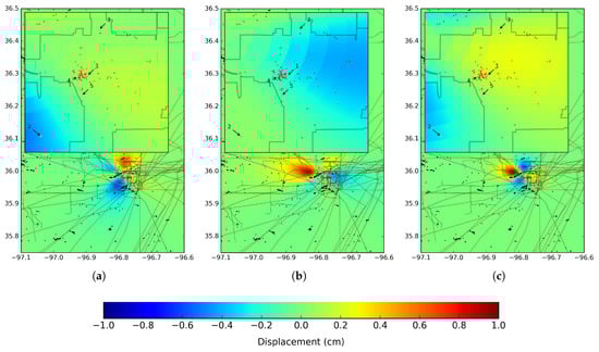
Figure 13.
Model displacement components overlaid with EERI damage data (red circles) and Federal Emergency Management Agency (FEMA) Hazards U.S. (HAZUS) oil (brown line) and gas (green line) pipeline data. Also plotted is relocated seismicity [5] (black dots), relocated Mw 5.0 epicenter [5] (orange-red star), and USGS Mw 5.0 epicenter (magenta star). The locations of buildings or infrastructure damaged by ground failure are plotted and labeled with a unique ID from Table 8. (a) North component. (b) East component. (c) Vertical component.
5. Discussion
Since the late 2015 lift on the 40-year ban on U.S. oil exports, a surge in U.S. shale oil production has strained pipeline and storage capacity. Surface displacement through an induced earthquake or through wastewater injection can damage this critical infrastructure, significantly impacting the U.S. economy and the environment. Our time series analysis reveals 4 to 6 cm of positive LOS displacement (uplift) over ∼17 months (June 2015 to November 2016), a double in the uplift rate presented by Loesch and Sagan [13] of 4.4 cm over ∼49 months (December 2006 to January 2011). Loesch and Sagan [13] use an SBAS time series analysis of Japan Aerospace Exploration Agency (JAXA) Advanced Land Observing Satellite (ALOS) Phased Array L-band Synthetic Aperture Radar (PALSAR) images to show a broad uplift signal spanning 4 km. Our regions of uplift generally overlap; however, their uplift signal extends northeast by approximately 1 km. The JAXA ALOS PALSAR time series has greater coherence than our S1A time series due its longer, L-band wavelength, minimizing interference with vegetation.
We propose that the cumulative wastewater injection from multiple wells into shallow layers is causing pore pressure increase and in turn regional uplift. In downtown Cushing, none of the wastewater injection wells within 6 km are injecting into or deeper than the Arbuckle formation. In this same region, we are seeing the greatest localized regional uplift. Figure 14 shows that, although regional uplift is caused by the 2015 earthquakes, the ground continues to uplift into our final cumulative displacement image.
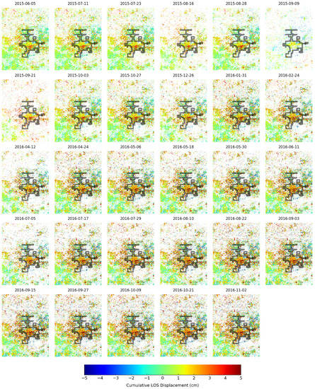
Figure 14.
Cumulative displacement time series slices overlaid with Cushing city boundary (gray outline).
We attribute the 2014, 2015, and 2016 sequences to deep wastewater injection into the Arbuckle formation by local wastewater injection wells. When wastewater was injected into the Arbuckle, the pore pressure increase reduced the effective normal stress on an existing fault, inducing slip. Another possible explanation is the combined pore pressure increase from injection into the Arbuckle and shallower formations resulted in a pore pressure gradient, facilitating in situ fluid to flow into existing faults within the Arbuckle. The fluid flow reduced the frictional strength of the fault, inducing slip [31].
Figure 15 presents injection data for all UIC wells within 10 km of downtown Cushing. Data for the resulting 33 UIC injection wells dates back to 2011. Although we cannot comment on the source of the regional uplift from 2006 to 2011, we do see a significant increase in total injected volume per month starting in 2014 and peaking in 2015. From 2011 to 2018, only a single UIC well, API 3511923843, injects at high-rates. The period at which API 3511923843 injects at high-rates into the Arbuckle immediately precedes the 2014 earthquake sequence.
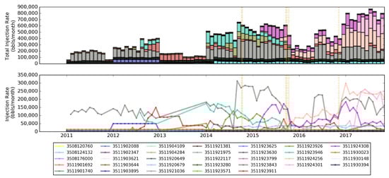
Figure 15.
Class II Underground Injection Control (UIC) injection rates for wells within 10 km of downtown Cushing.
Our inversion suggests the depth of the 2016 Mw 5.0 earthquake is much shallower than that of the USGS model. The shallower source is in agreement with the Schoenball and Ellsworth [5] depth estimate of 3.625 km within the crystalline basement. Past studies [32,33,34] have attributed the discrepancy between seismic and geodetic source depths to the coarse approximation for the uppermost crust of the elastic halfspace model that does not consider possible rigidity contrasts. However, the observed MMI VII damage in downtown Cushing further supports a shallower source depth.
6. Conclusions
In our study, we characterize the impact of wastewater injection on the city of Cushing and its critical national infrastructure using DInSAR. In terms of long-term deformation, we observe 4 to 6 cm of regional uplift across the city over 17 months (Figure 16). We also successfully observe instantaneous, coseismic deformation from the 2016 Mw 5.0 earthquake. This is the best example of coseismic deformation associated with a moderate (5.0 ≤ M ≤ 5.9), shallow induced earthquake to date. Although the 2016 Mw 5.0 earthquake was too small to cause major infrastructure damage related to permanent displacement, a larger earthquake at this depth could have significant impacts. Following a magnitude 4.8–5.3 earthquake, the Oklahoma Department of Transportation (ODOT) mandates a 15-mile inspection radius from the epicenter of roads and bridges. Using critical infrastructure data in conjunction with high-resolution horizontal and vertical displacement maps derived from DInSAR can help identify those locations within such a large area that need to be prioritized for mitigation or remediation. Our source inversion demonstrates the potential for InSAR to facilitate rapid response efforts for shallow, moderate-sized earthquakes, especially in poorly seismically-instrumented areas.
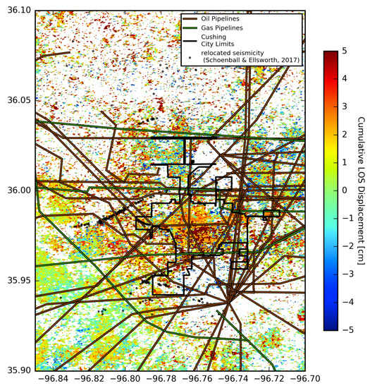
Figure 16.
Cumulative displacement overlaid with at risk FEMA HAZUS critical infrastructure.
Author Contributions
DInSAR construction and analysis by M.B.; damage data acquisition and analysis by B.W.B., coseismic inversion by M.B., visualizations by M.B., writing by M.B. and B.W.B., supervision by K.F.T. and A.B.L., funding acquisition by K.F.T. and A.B.L.
Funding
This research was funded by the National Science Foundation award number 1520846.
Acknowledgments
We would like to acknowledge four anonymous reviewers for their constructive comments and feedback. FEMA HAZUS data provided by NASA-EDECIDER. Relocated seismic data published in Schoenball and Ellsworth [5]. UIC Class II well data provided by the Oklahoma Corporation Commission (OCC) [27]. Reconnaissance data downloaded from EERI Clearinghouse website [16]. S1A SLCs and orbit data provided by ESA. S1A SLC data downloaded from the Alaska Satellite Facility (ASF) using the UNAVCO Seamless SAR Archive (SSARA) API. Oklahoma fault database downloaded from the Oklahoma Geological Survey [15]. Rivers, streams, and waterbody data is from the USGS National Hydrography Dataset. Ten-meter USGS NED DEM and 30 meter SRTM v.3 DEM downloaded from https://nationalmap.gov/elevation.html. 2014 moment tensor (MT) solutions obtained from McNamara et al. [3], 2015 M4.0 MT obtained from the St. Louis University North America MT catalog [35], and 2015 M4.1 and M4.3 and 2016 5.0 MT solutions obtained from USGS. The USGS National Earthquake Information Center moment tensors acquired from https://earthquake.usgs.gov/earthquakes/eventpage/us100075y8. Oklahoma municipal boundaries from the Oklahoma Office of Geographic Information OKMaps (https://okmaps.org/OGI/). Introductory figure made using Generic Mapping Tools v. 4.5.16 [36] and damage data figures made using QGIS v. 2.18.9 [37]. SAR data processed using ISCE software [17] v. 2.2.0 available through UNAVCO at http://winsar.unavco.org/isce.html or through the JPL Office of Technology Transfer http://ott.jpl.nasa.gov/index.php?page=software. DInSAR time series made using GIAnT software [21] v. 1.0 available from Caltech under a public license at http://earthdef.caltech.edu. Inversion completed using Pyrocko software [28] v. 2018.01.29 available at https://pyrocko.org.
Conflicts of Interest
The authors declare no conflict of interest.
Appendix A
The phase coherence images overlaid with municipal boundaries (Figure A1) show that the municipals are areas of consistent coherence. To avoid processing bias, we construct a time series using a reference region of 100 by 100 meters within the municipal boundary of Carney, OK, USA.

Figure A1.
Phase coherence images for preseismic pairs overlaid with municipal boundaries.
The wrapped coseismic interferograms for the 2016 Mw 5.0 earthquake (Figure A2), when compared to the unwrapped coseismic interferograms, can highlight unwrapping errors. No significant unwrapping errors are present in our coseismic unwrapped interferograms.

Figure A2.
Wrapped coseismic interferograms for 2016 Mw 5.0 Cushing earthquake.
References
- Sircar, S.; Power, D.; Randell, C.; Youden, J.; Gill, E. Lateral and Subsidence Movement Estimation Using InSAR. IGARSS 2004, 2991–2994. [Google Scholar] [CrossRef]
- Luza, K.V.; Madole, R.F.; Crone, A.J. Investigation of the Meers Fault in Southwestern Oklahoma. Oklahoma Geol. Surv. Spec. Publ. 1987, 87-1, 58. [Google Scholar]
- McNamara, D.E.; Hayes, G.P.; Benz, H.M.; Williams, R.A.; McMahon, N.D.; Aster, R.C.; Holland, A.; Sickbert, T.; Herrmann, R.; Briggs, R.; et al. Reactivated faulting near Cushing, Oklahoma: Increased potential for a triggered earthquake in an area of United States strategic infrastructure. Geophys. Res. Lett. 2015, 42, 8328–8332. [Google Scholar] [CrossRef]
- McGarr, A.; Barbour, A.J. Wastewater disposal and the earthquake sequences during 2016 near Fairview, Pawnee, and Cushing, Oklahoma. Geophys. Res. Lett. 2017, 44, 9330–9336. [Google Scholar] [CrossRef]
- Schoenball, M.; Ellsworth, W.L. Waveform-relocated earthquake catalog for Oklahoma and Southern Kansas illuminates the regional fault network. Seismol. Res. Lett. 2017, 88, 1252–1258. [Google Scholar] [CrossRef]
- Schoenball, M.; Ellsworth, W.L. A systematic assessment of the spatiotemporal evolution of fault activation through induced seismicity in Oklahoma and Southern Kansas. J. Geophys. Res. Solid Earth 2017, 122, 10189–10206. [Google Scholar] [CrossRef]
- Taylor, J.; Çelebi, M.; Greer, A.; Jampole, E.; Masroor, A.; Melton, S.; Norton, D.; Paul, N.; Wilson, E.; Xiao, Y. EERI Earthquake Reconnaissance Team Report: M5.0 Cushing, Oklahoma, USA Earthquake on November 7, 2016; EERI: Oakland, CA, USA, 2017. [Google Scholar]
- Ellsworth, W.L. Injection-induced earthquakes. Science 2013, 341, 1225942. [Google Scholar] [CrossRef] [PubMed]
- Walsh, F.R.; Zoback, M.D. Oklahoma’s recent earthquakes and saltwater disposal. Sci. Adv. 2015, 1, e1500195. [Google Scholar] [CrossRef] [PubMed]
- Weingarten, M.; Ge, S.; Godt, J.W.; Bekins, B.A.; Rubinstein, J.L. High-rate injection is associated with the increase in U.S. mid-continent seismicity. Science 2015, 348, 1336–1340. [Google Scholar] [CrossRef] [PubMed]
- Hincks, T.; Aspinall, W.; Cooke, R.; Gernon, T. Oklahoma’s induced seismicity strongly linked to wastewater injection depth. Science 2018, 359, 1251–1255. [Google Scholar] [CrossRef] [PubMed]
- Grandin, R.; Vallée, M.; Lacassin, R. Rupture process of the M w 5.8 Pawnee, Oklahoma, earthquake from Sentinel-1 InSAR and seismological data. Seismol. Res. Lett. 2017, 88, 994–1004. [Google Scholar] [CrossRef]
- Loesch, E.; Sagan, V. SBAS analysis of induced ground surface deformation from wastewater injection in east central Oklahoma, USA. Remote Sens. 2018, 10, 283. [Google Scholar] [CrossRef]
- Fielding, E.J.; Sangha, S.S.; Bekaert, D.P.S.; Samsonov, S.V.; Chang, J.C. Surface deformation of north-central Oklahoma related to the 2016 Mw 5.8 Pawnee earthquake from SAR interferometry time series. Seismol. Res. Lett. 2017, 88, 971–982. [Google Scholar] [CrossRef]
- Holland, A.A. Preliminary Fault Map of Oklahoma; Oklahoma Geological Survey: Norman, OK, USA, 2015. [Google Scholar]
- Earthquake Engineering Research Institute (EERI). EERI Oklahoma Photo Gallery; EERI: Oakland, CA, USA, 2016; Available online: http://www.eqclearinghouse.org/2016-09-03-oklahoma/maps-and-photos/photo-gallery/ (accessed on 21 October 2018).
- Rosen, P.A.; Gurrola, E.M.; Franco Sacco, G.; Zebker, H.A. The InSAR Scientific Computing Environment. In Proceedings of the 9th European Conference on Synthetic Aperture Radar, Nuremberg, Germany, 23–26 April 2012. [Google Scholar]
- Chen, C.W.; Zebker, H.A. Network approaches to two-dimensional phase unwrapping: intractability and two new algorithms. J. Opt. Soc. Am. A 2000, 17, 401. [Google Scholar] [CrossRef]
- Chen, C.; Zebker, H. Two-dimensional phase unwrapping with statistical models for nonlinear optimization. IGARSS 2000 2000, 7, 3213–3215. [Google Scholar] [CrossRef]
- Chen, C.W.; Zebker, H.A. Phase unwrapping for large SAR interferograms: Statistical segmentation and generalized network models. IEEE. T. Geosci. Remote 2002, 40, 1709–1719. [Google Scholar] [CrossRef]
- Agram, P.S.; Jolivet, R.; Riel, B.; Lin, Y.N.; Simons, M.; Hetland, E.; Doin, M.P.; Lasserre, C. New radar interferometric time series analysis toolbox released. EOS 2013, 94, 69–70. [Google Scholar] [CrossRef]
- Doin, M.P.; Lodge, F.; Guillaso, S.; Jolivet, R.; Lasserre, C.; Ducret, G.; Grandin, R.; Pathier, E.; Pinel, V. Presentation of the small baseline NSBAS processing chain on a case example: The Etna deformation monitoring from 2003 to 2010 using Envisat data. In Proceedings of the ESA Fringe 2011 Workshop, Frascati, Italy, 19–23 September 2011. [Google Scholar]
- Wood, H.O.; Neumann, F. Modified mercalli intensity scale of 1931. B. Seismol. Soc. Am. 1931, 21, 277–283. [Google Scholar]
- Wald, D.J.; Quitoriano, V.; Dengler, L.A.; Dewey, J.W. Utilization of the internet for rapid community intensity maps. Seismol. Res. Lett. 1999, 70, 680–697. [Google Scholar] [CrossRef]
- Wald, D.J.; Dewey, J.W. Did You Feel It? Citizens Contribute to Earthquake Science; U.S. Geological Survey: Reston, VA, USA, 2005.
- Wald, D.J.; Quitoriano, V.; Worden, B.; Hopper, M.; Dewey, J.W. USGS “Did You Feel It?” internet-based macroseismic intensity maps. Ann. Geophys. 2011, 54, 688–707. [Google Scholar] [CrossRef]
- Oklahoma Corporation Commission (OCC). Oklahoma Corporation Commission Oil and Gas Datafiles; Oklahoma Corporation Commission: Oklahoma, OK, USA, 2018. [Google Scholar]
- Pyrocko.org: Software for Seismology. Available online: https://pyrocko.org (accessed on 21 October 2018).
- Kramer, S.L.; Stewart, J.P. Geotechnical aspects of seismic hazards. In Earthquake Engineering: From Engineering Seismology to Performance-Based Engineering; Bozorgnia, Y., Bertero, V.V., Eds.; CRC Press: Boca Raton, FL, USA, 2004; Chapter 4; pp. 1–85. [Google Scholar] [CrossRef]
- Zalachoris, G.; Rathje, E.M.; Paine, J.G. V S30 Characterization of Texas, Oklahoma, and Kansas Using the P-Wave Seismogram Method. Earthq. Spectra 2017, 33, 943–961. [Google Scholar] [CrossRef]
- Brown, M.R.M.; Ge, S. Short note distinguishing fluid flow path from pore pressure diffusion for induced seismicity. Bull. Seismol. Soc. Am. 2018. [Google Scholar] [CrossRef]
- Ganas, A.; Kourkouli, P.; Briole, P.; Moshou, A.; Elias, P.; Parcharidis, I. Coseismic displacements from moderate-size earthquakes mapped by Sentinel-1 differential interferometry: The case of February 2017 Gulpinar Earthquake Sequence (Biga Peninsula, Turkey). Remote Sens. 2018, 10, 1089. [Google Scholar] [CrossRef]
- Amoruso, A.; Crescentini, L.; Fidani, C. Effects of crustal layering on source parameter inversion from coseismic geodetic data. Geophys. J. Int. 2004, 159, 353–364. [Google Scholar] [CrossRef]
- Cattin, R.; Briole, P.; Lyon-Caen, H.; Bernard, P.; Pinettes, P. Effects of superficial layers on coseismic displacements for a dip-slip fault and geophysical implications. Geophys. J. Int. 1999, 137, 149–158. [Google Scholar] [CrossRef]
- Herrmann, R. St. Louis University North America Moment Tensor catalog. Available online: http://www.eas.slu.edu/eqc/eqc_mt/MECH.NA/ (accessed on 21 October 2018).
- Wessel, P.P.; Smith, W.H.F. Generic Mapping Tools Graphics. 2004. Available online: http://gmt.soest.hawaii.edu/ (accessed on 21 October 2018).
- QGIS Development Team. QGIS Geographic Information System. Open Source Geospatial Foundation Project; OSGeo: Chicago, IL, USA, 2018. [Google Scholar]
© 2018 by the authors. Licensee MDPI, Basel, Switzerland. This article is an open access article distributed under the terms and conditions of the Creative Commons Attribution (CC BY) license (http://creativecommons.org/licenses/by/4.0/).