A Demand Prediction-Driven Algorithm for Dynamic Shared Autonomous Vehicle Relocation: Integrating Deep Learning and System Optimization

Abstract

This paper develops a dynamic repositioning mechanism for shared autonomous vehicles (SAVs) driven by travel demand. A prediction model for SAV travel demand is constructed by the proposed GRU-FC network. On this basis, an integer programming model for empty-vehicle dispatching which aims to maximize the SAV revenue while minimizing the costs of vehicle relocation and operation is formulated. The results indicate that, relative to relying solely on natural vehicle dispatching, the proposed dispatching scheme reduces empty vehicle dispatches by 21.00% and increases total system profit by 38.89%. The findings theoretically improve the dynamic optimization theory of SAV dispatching and provide theoretical support for algorithm design based on the “demand-pull” principle. The method proposed in this paper is beneficial to optimizing the dynamic vehicle dispatching theory of SAVs. It helps to boost system revenue, reduce empty driving costs, alleviate traffic pressure, and lower energy consumption and environmental pollution, thereby fostering sustainable urban mobility and supporting the Sustainable Development Goals of clean energy and sustainable cities.

1. Introduction

As an emerging mode of intelligent transportation, shared autonomous vehicles (SAVs) possess significant technological advantages and application potential [1]. Firstly, they eliminate the need for human drivers, which not only reduces labor costs but also enables more optimized in-vehicle space layouts to accommodate a greater number of passengers, thereby enhancing resource utilization efficiency [2]. For example, a simulation study by Fagnant and Kockelman [3] demonstrated that SAVs can reduce operational labor expenses by approximately 70%. Secondly, being free from the influence of drivers’ subjective preferences in route selection, SAVs can leverage intelligent decision-making systems to achieve globally optimal driving route planning [4]. Thirdly, SAVs offer continuous operational capability, meaning they can operate non-stop 24 h a day. As shown in the Austin case study by Fagnant and Kockelman [5], the stability of vehicle supply during peak hours has improved by over 40% compared to traditional models, thus avoiding supply shortages caused by issues such as driver shift changes during peak periods. However, SAVs encounter challenges in empty vehicle dispatching during actual operations. Particularly in large-scale operation scenarios, the rationality of dispatching algorithms directly impacts system efficiency. Inefficient algorithms may result in a series of problems, including escalating operational costs, delayed fulfillment of passenger demands, and increased energy consumption and pollutant emissions [6,7].

Traditional shared cars, specifically referring to ride-hailing taxis operating in most cities in China, rely primarily on drivers’ subjective decision-making for empty-vehicle cruising and relocation. During daytime operational periods, after completing a trip (dropping off passengers at the destination), drivers independently decide where to cruise or wait to accept new orders. This empty-vehicle movement (from the drop-off point of the previous trip to the pick-up point of the next trip) is a passive relocation process determined by individual drivers’ judgments rather than a centralized scheduling system. In this paper, this driver-led, non-centralized empty-vehicle movement is defined as natural empty-vehicle dispatching. However, with the proposal of the SAV concept and its pilot operations in certain cities, the lack of efficient empty-vehicle relocation strategies have emerged as a critical issue requiring urgent breakthroughs. Current mainstream relocation schemes [8] mostly adopt static algorithms, which calculate daily travel generation by considering historical travel volume, land use attributes of each district, population size, and other factors. These static algorithms, focused on minimizing total driving costs during dispatching, involve determining the relocation plan for each district, with greater emphasis on generating the most cost-effective driving routes in the subsequent path decision-making phase. Moreover, most of these schemes complete empty-vehicle transfer during non-operational periods (e.g., at night). During the operational period, empty driving from the drop-off point of the previous trip to the pick-up point of the next trip—referred to as natural dispatching in this paper—enables the natural relocation of vehicles. However, such non-real-time dispatching modes may result in significant supply–demand mismatch issues, such as insufficient vehicles during peak hours and in peak areas, while there are still surplus vehicles during off-peak hours and in off-peak areas. This further leads to problems including increased operating costs, loss of passengers, and a decrease in the overall attractiveness of the SAV system. Therefore, exploring dynamic relocation algorithms has become an inevitable requirement for enhancing the operational efficiency and service quality of SAVs.

SAVs are centered on serving passengers, with their service response speed and the extent of alignment with passenger demands directly determining the system’s market share and overall benefits. Accordingly, empty-vehicle relocation must prioritize meeting passengers’ travel demands as its core goal, and the fundamental logic of its algorithm design should adhere to the “demand-driven” principle [9]. Specifically, vehicles are dynamically allocated based on real-time and predicted travel demands to achieve precise deployment of empty vehicles across both temporal and spatial dimensions, thereby ensuring a dynamic balance between supply and demand. Concurrently, the cost factor in vehicle dispatching cannot be overlooked [10]. Optimizing dispatching strategies to reduce empty driving distance not only lowers operational costs but also effectively eases the pressure of empty-vehicle dispatching on road traffic, reduces energy consumption and environmental pollution [11], and realizes the coordinated enhancement of economic and social benefits. It follows that the design of SAV empty-vehicle dispatching algorithms needs to comprehensively address the core demands of both the demand and supply sides. Given this context, this paper will develop an optimal dynamic empty-vehicle relocation model aimed at maximizing the total system’s benefits, building upon SAV travel demand prediction.

The main contributions of this paper are as follows:

• A dynamic empty-vehicle relocation mechanism driven by demand prediction is developed to enable hourly demand response, facilitating supply–demand matching of SAVs across both temporal and spatial dimensions. By taking the maximization of system benefits as its objective, the mechanism allows the system to balance the interests of both the supply and demand sides. This hourly dynamic mechanism achieves finer-grained demand adaptation and avoids supply–demand mismatches in peak hours/areas.
• Leveraging the time continuity evolution characteristics and segment similarity features of trip distribution, a deep learning method that combines Gated Recurrent Unit (GRU) and Fully Connected Layers (FC Layers)—incorporating both time series capture and feature extraction—is proposed to achieve accurate prediction of SAV travel demand. Compared with single-model prediction (overreliance on historical OD data or lack of temporal dependencies), it captures long-term temporal rules and multi-dimensional correlations simultaneously, addressing traditional prediction’s staticity and lag to support real-time relocation.

The remaining chapters of this paper are structured as follows: Section 2 provides a review of existing related research. Section 3 establishes the SAV dynamic empty-vehicle relocation model and the travel volume prediction model. Section 4 employs actual online car-hailing data from Shenzhen City, China, for case analysis and method validation, and Section 5 presents conclusions and discusses future research directions.

2. Related Works

2.1. Methods of Empty-Vehicle Relocation

Traditional empty-vehicle relocation methods have certain limitations in timeliness and dynamic adaptability. In terms of scheduling cycles, several studies indicate that past practices predominantly adopted a daily static scheduling mode [12,13,14]. For instance, Yang et al. [15] focused on shared car operations and observed that they relied on centralized nighttime scheduling. While this approach can balance vehicle distribution to a certain extent, it fails to promptly respond to real-time and fluctuating demands during daytime operational periods, such as the sudden surge in ride demand in commercial areas during peak hours. This delayed scheduling results in supply–demand imbalances in specific regions, prolonged passenger waiting times, elevated order cancelation rates, and passenger attrition, which severely undermines the market competitiveness of the SAV system. Similarly, the scheduling model proposed by Nourinejad et al. [16] is based on fixed cycles, making it ineffective in addressing dynamic demand fluctuations.

In terms of scheduling strategies, most traditional methods prioritize minimizing total scheduling distance as their core objective. The inter-regional empty-vehicle allocation model developed by Nourinejad et al. [16] implements supplementary relocation based on vehicle ownership thresholds in fixed districts, adhering to such static strategies. It only presets vehicle quantities in each district using historical data and does not incorporate real-time travel volume to establish a dynamic adjustment mechanism. Studies by Jorge et al. [17] and Huang et al. [18,19] also employ similar static strategies, which struggle to flexibly adapt to rapid short-term demand changes, leading to a disconnect between scheduling schemes and actual operational scenarios.

2.2. Methods of SAV Travel Demand Prediction

The accuracy of travel demand prediction is directly related to the effectiveness of empty-vehicle relocation strategies [20]. However, current prediction methods have failed to effectively overcome the issues of static nature and lag in prediction results. In terms of model construction, traditional prediction models mostly rely on historical OD data and land use characteristics [21,22]. For instance, Repoux et al. [23] used a Markov model to predict the future state of stations based on historical order data. While this approach offers some predictive value, it fails to fully integrate dynamic variables such as real-time traffic flow and weather, resulting in notable deviations in prediction results during peak hours or in scenarios such as special weather conditions. Vateekul et al. [24] combined the Discrete Choice Model (DCM) and Deep Neural Network (DNN) in travel behavior research, which improved the prediction ability for some travel decisions but still could not cope with the dynamically complex demands of SAV travel scenarios. Additionally, recent studies have focused on optimizing the efficiency of deep convolutional neural network (CNN)-based models, which are widely used in feature extraction for demand prediction or image-related traffic tasks. For example, Zhang et al. [25] proposed a Wavelet-Based Physically Guided Normalization Dehazing Network (WBPGNDN), which enhances model speed and processing quality through frequency domain learning. This logic provides valuable insights for improving the efficiency of CNN-related feature extraction modules, e.g., fully connected layers in hybrid networks, in SAV travel demand prediction, addressing the potential issue of low inference speed in traditional CNN-based models.

2.3. Literature Summary

Based on the above analysis, we can see that research progress in SAV-related studies can be summarized across three key areas: In SAV empty-vehicle relocation, studies focus more on static schemes than dynamic algorithms. Static schemes rely on non-operational transfers and natural dispatching, with the goal of minimizing costs. Dynamic algorithms focus on improved demand fulfillment, while hub-based models achieve supply–demand balance through multi-modal integration. For demand prediction, methods have advanced from traditional statistical models which depend on historical data to deep learning. Deep learning approaches include single models for feature or temporal mining, CNNs for spatial extraction, and hybrid frameworks. In system optimization, research covers single-dimensional goals such as cost or wait time reduction and limited multi-dimensional efforts focusing on revenue-cost balance, which verify SAVs’ mobility potential.

Despite this progress, there are still significant synergistic deficiencies in the empty-vehicle relocation and travel demand prediction of SAVs. On the one hand, traditional relocation modes are limited by the daily relocation cycle and static supplementary strategies and cannot respond in a timely manner to real-time demand changes during the operation period, leading to reduced system attractiveness due to passenger attrition. On the other hand, the static tendency of travel demand prediction methods, which do not carry out rolling empty-vehicle relocation based on dynamic travel volume, makes it difficult to effectively support dynamic relocation decisions. Moreover, previous studies have focused on empty-vehicle relocation with the goal of minimizing the total relocation distance. A summary of recent related studies is shown in Table 1.

Table 1. Summary of the key literature on SAV operation and management.

Research Direction	Core Research Progress	Existing Gaps	Representative Literature
SAV Empty-Vehicle Relocation	Static schemes dominate: daily scheduling cycles, fixed-district thresholds, distance minimization. Dynamic algorithms boost demand fulfillment; hub models integrate multi-modal dynamics.	Static schemes fail to respond to real-time demand, causing imbalance and passenger loss. Dynamic/hub models lack real-time applicability or demand coupling.	[12,13,14,15,16,17,18,19,21]
SAV Travel Demand Prediction	From historical-data-based statistical models to deep learning. Deep learning: single models for feature/temporal mining, CNNs for spatial extraction, optimized CNN efficiency.	Traditional models lack dynamic variables. Deep learning lacks feature synergy or SAV adaptation.	[23,24,25]
System Optimization	Single-dimensional goals: cost, wait time, distance. Limited multi-dimensional revenue–cost balance. Verifies SAV mobility potential.	Single-dimensional optimization dominates. No system benefits consensus; lack of relocation–prediction synergy.	[20,22]

Therefore, this paper will construct a dynamic empty-vehicle relocation mechanism driven by travel demand prediction. By adopting a deep learning method that combines GRU and Fully Connected Layer, it will capture the time continuity evolution characteristics and segment similarity features of travel demand, and establish a high-precision model for predicting SAV travel demand to break through the static limitations of traditional prediction methods. On this basis, an integer programming model for empty-vehicle relocation will be constructed with the goal of maximizing system benefits, so as to realize hourly dynamic demand response. This will generate empty-vehicle relocation schemes that can accurately match real-time demands in temporal and spatial dimensions, and promote the dynamic balance between supply and demand of the SAV system.

3. Modeling

3.1. Problem Analysis

Our research focuses on empty-vehicle relocation for all SAVs within an urban area. Considering the total number of taxis and the quantity of pick-up/drop-off points in existing cities, spatially refining calculation results to the number of vehicles at each individual pick-up/drop-off hotspot would lead to enormous computing resource consumption due to the excessive number of such points and their even more numerous pairings. Therefore, for such large-scale, city-wide empty-vehicle relocation, we will relax the spatial granularity to the district level. Specifically, assuming there are $N$ districts, the output will be the volume of empty-vehicle relocation between any two districts $i$ and $j$.

In addition, since ride-sharing is one of the characteristics of SAVs, this paper needs to define the mode of ride-sharing. Generally, SAV and online car-hailing services currently mostly adopt the static ride-sharing mode, where all passengers are matched for ride-sharing by the platform before their trips begin. In contrast, the dynamic ride-sharing mode refers to the type where passengers who are already in transit or about to start their trips receive and agree to ride-sharing requests from other passengers during their journey. To simplify the model and align with the current operational rules of SAVs, this paper assumes the adoption of the static ride-sharing mode. This assumption is not only consistent with the operational status of most current SAV pilots and ride-hailing platforms but also helps focus the study on the core goal of optimizing empty-vehicle relocation. Its operational schematic diagram is shown in Figure 1.

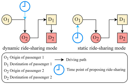
Figure 1. Schematic diagram of ride-sharing modes.

The core objective of the empty-vehicle relocation algorithm is to align the number of vehicles deployed in each district with its anticipated demand for the next time period. Specifically, higher demand signals greater importance within the transportation network, necessitating more vehicles; conversely, lower demand corresponds to lower importance, allowing for fewer deployments. Beyond satisfying passenger travel needs, the key consideration is identifying a relocation scheme that maximizes overall system benefits. To this end, the SAV system encompasses both supply and demand perspectives: passenger benefits are primarily derived from successful trip completion, while operational costs include energy consumption and vehicle maintenance. These factors are closely linked to fleet size, pricing, ride-sharing occupancy, travel volume, and inter-district relocation volumes, with the hourly relocation volume between districts serving as the key decision variable in this study. The proposed model aims to match post-relocation empty-vehicle distribution with passenger demand patterns, thereby fulfilling travel requirements. The fundamental logic of empty-vehicle relocation is illustrated in Figure 2 and Figure 3.

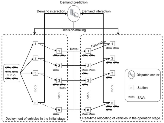
Figure 2. Schematic diagram of empty-vehicle dispatching process.

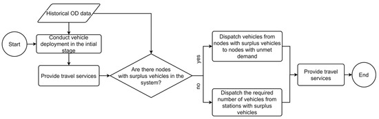
Figure 3. Vehicle relocating decision flowchart.

3.2. Method Selection

Based on several issues in the existing research summarized in Section 2, this paper proposes a model framework that integrates GRU-FC-based travel demand forecasting with an integer programming model for dynamic SAV relocation. Among the framework components, the upper-layer GRU-FC model captures the temporal continuity evolution characteristics of SAV demand via GRU and extracts multi-dimensional key features through the FC Layer. This enables accurate prediction of demand distribution in future time periods, providing data support for formulating scheduling schemes in advance and effectively addressing the problem of lagging demand forecasting. The lower-layer integer programming model takes maximizing total system benefits as its core objective, integrating passenger travel revenue, empty-vehicle energy consumption costs, and vehicle maintenance costs. Meanwhile, it ensures that the vehicle supply in each district meets the minimum demand through the constraint of safe vehicle quantity, reducing the empty driving rate while guaranteeing the passenger order completion rate, thus solving the dilemma of unbalanced benefits caused by single scheduling objectives. The combination of the upper and lower layers forms an hourly dynamic response mechanism: based on the hourly demand forecasts from the GRU-FC model, the integer programming model updates the inter-district empty-vehicle scheduling schemes on an hourly basis, achieving fine-grained matching of supply and demand in both temporal and spatial dimensions and addressing the temporal–spatial mismatch problem caused by traditional coarse-grained scheduling.

3.3. Parameter Calculation and Model Constraint

Firstly, we need to define the key variable of relocation points. For the convenience of calculation, each district is replaced by its centroid, and it is assumed that all vehicles departing from and arriving at any district are directed to this centroid. Therefore, according to the overall zoning of the area to be studied, assuming there are $N$ districts, then there are a corresponding $N$ stations. Further, a set of departure points (or arrival points) for SAVs is established as $\mathbf{N}=\{1,2,3,i,j,\dots ,N\}$, where $i$ and $j$ are different stations in the station set. Then, we define the deployment scale of a station at the initial moment as $n_i^0$, whose physical meaning is the number of vehicles deployed at station $i$ at time period $t=0$. Here, $t$ is the time period count, and its set is $\mathbf{T}=\{0,1,2\dots ,23\}$, with an interval of 1 h between adjacent $t$ values. And $n_{sav}$ is the total number of available shared autonomous vehicles.

The initial deployment scale $n_i^0$ of station $i$ is constrained by the total number of available shared autonomous vehicles, as shown in Formula (1).

$$\sum _{i\in \mathbf{N}}{n}_i^0=n_{sav}$$

(1)

As for travel volume, $w_{ijk}^t$ is defined as the SAV travel volume of ride-sharing passengers with $k$ people departing from station $i$ to station $j$ at the start of time period $t$. In particular, when $k=0$, this variable represents the relocation volume, denoted as $w_{ij0}^t$, which indicates the travel volume with 0 passengers moving from station $i$ to station $j$ during time period $t$ under the command of the dispatch center.

Regarding the number of ride-sharing passengers (k) mentioned above, the SAVs studied in this paper are assumed to be standard passenger vehicles widely used in the current market with a maximum passenger capacity of 5 people, so the number of ride-sharing passengers per vehicle $k$ belongs to the set $\mathrm{K}=\{0,1,2,3,4,5\}$.

Based on previous travel behavior analysis and modeling experience [26], it is known that the greater the travel volume in a certain area, the greater its travel supply, and the two are basically proportional. And higher travel demand in a district corresponds to a greater need for initial vehicle deployment. Therefore, in this paper, the proportion of the SAV deployment scale in the total number of vehicles $n_{sav}$ is determined according to the proportion of the SAV travel volume at a certain station at a certain time to the total travel volume. We define ${\epsilon }_i$ as the weight of the initial vehicle deployment scale at station $i$, which reflects the importance of station $i$ in the urban transportation network. Then,

$${\epsilon }_i=\sum _t^{\mathbf{T}}\sum _{j\in \mathbf{N}\backslash \left\{i\right\}}\sum _{k=1}^{\mathbf{K}}{w}_{ijk}^t/\sum _t^{\mathbf{T}}\sum _{i\in \mathbf{N}}\sum _{j\in \mathbf{N}\backslash \left\{i\right\}}\sum _{k=1}^{\mathbf{K}}{w}_{ijk}^t$$

(2)

where $w_{ijk}^t$ represents the travel volume of $k$ ride-sharing passengers departing from station $i$ to station $j$ at the start of time period $t$.

After obtaining ${\epsilon }_i$ via Formula (2), we can further calculate the initial vehicle deployment at each station using Formula (3). This step connects travel demand characteristics with initial resource allocation, forming the starting point of the entire dynamic relocation logic—without this weight calculation, the initial vehicle layout would lack demand-oriented guidance and lead to more frequent subsequent relocations.

$$n_i^0={\epsilon }_i{n}_{sav},\forall i\in \mathbf{N}$$

(3)

We define the number of vehicles at station $i$ at the start of time period $t$ as $n_i^t$. It is equal to the number of vehicles at station $i$ at the start of time period $(t-1)$ plus the number of vehicles arriving at station $i$ from other stations, minus the number of vehicles departing from station $i$, that is,

$$n_i^t=n_i^{t-1}+\sum _k^{\mathbf{K}}\sum _{j\in \mathbf{N}\backslash \left\{i\right\}}{w}_{jik}^{t-1}-\sum _k^{\mathbf{K}}\sum _{j\in \mathbf{N}\backslash \left\{i\right\}}{w}_{ijk}^{t-1},\forall i\ne j\in \mathbf{N},t\in \mathbf{T}$$

(4)

$n_i^t$ shall be positive, and the travel volume departing from any station shall not exceed the number of vehicles at that station.

$$n_i^t\ge 0,\forall i\in \mathbf{N},t\in \mathbf{T}$$

(5)

$$\sum _k^{\mathbf{K}}\sum _{j\in \mathbf{N}\backslash \left\{i\right\}}{\sigma }_k{w}_{ijk}^t\le n_i^t,\forall i\ne j\in \mathbf{N},t\in \mathbf{T}$$

(6)

where ${\sigma }_k$ is the weight of vehicles with $k$ ride-sharing passengers in the total number of travel vehicles (excluding relocation vehicles), which reflects passengers’ preference for the number of ride-sharing passengers.

We propose the concept of the safe number of vehicles, that is, the number of vehicles at station $i$ in time period $t$ that meets the minimum travel demand, denoted as ${\mathit{ns}}_i^t$. If the number of vehicles at station $i$ in the next time period $(t+1)$ is less than the safe number of vehicles, it is necessary to relocate empty vehicles to station $i$ from other stations. We define ${\mathit{ns}}_i^t$ as the average travel volume of station $i$ in the future $(\tau -t+1)$ time periods, that is,

$${ns}_i^t={\displaystyle \frac{{\sum }_t^{\tau }{\sum }_{k=1}^{\mathbf{K}}{\sum }_{j\in \mathbf{N}\left\{i\right\}}{w}_{ijk}^t}{\tau -t+1}},\forall i\in \mathbf{N},t<\tau \in \mathbf{T}$$

(7)

where $\tau$ refers to a certain time period after time period $t$. The safety vehicle quantity is calculated by averaging the total travel volume in district i over the future time periods (τ − t + 1). The division by (τ − t + 1) converts the total demand into an average demand per time period. This logic aligns with the actual operation scenario where SAVs circulate continuously, and the average demand can reasonably reflect the minimum vehicle number needed to cover periodic demand without excessive redundancy.

The ${\mathit{ns}}_i^t$ calculated from Formula (7) will be compared with the real-time vehicle number $n_i^t$, which is updated via Formula (4), to identify stations with vehicle surpluses or deficits. This comparison is the premise for determining the relocation volume in Formula (8) and (9), bridging the gap between demand prediction and practical empty-vehicle scheduling in the overall calculation logic.

We determine the number of vehicles to be relocated from station $i$ to station $j$ ($w_{ij0}^t$) based on the relationship between the number of vehicles at each of the two stations and their respective safe numbers of vehicles.

In time period $t$, if the number of vehicles at station $i$ is greater than its safe number of vehicles, and the number of vehicles at station $j$ is less than its safe number of vehicles, then the relocation volume of SAVs dispatched from station $i$ to station $j$ ($w_{ij0}^t$) shall not exceed the number of vehicles at station $i$ that is in excess of its safe number. That is,

$$\sum _{j\in \mathbf{N}\backslash \left\{i\right\}}{w}_{ij0}^t\le n_i^t-{ns}_i^t,n_i^t\ge {ns}_i^t,n_j^t\le {ns}_j^t,\forall i\ne j\in \mathbf{N},t\in \mathbf{T}$$

(8)

If the number of vehicles at station $i$ in time period $t$ is greater than its safe number of vehicles, and the number of vehicles at station $j$ is less than its safe number of vehicles, then the relocation volume dispatched from station $i$ to station $j$ ($w_{ij0}^t$) is equal to the difference between the safe number of vehicles at station $j$ and the actual number of vehicles there.

$$\sum _{i\in \mathbf{N}\backslash \left\{j\right\}}{w}_{ij0}^t={ns}_j^t-n_j^t,n_i^t\ge {ns}_i^t,n_j^t\le {ns}_j^t,\forall i\ne j\in \mathbf{N},t\in \mathbf{T}$$

(9)

Formula (8) and (9) work in tandem: Formula (8) sets the upper limit of relocatable vehicles from surplus stations, while Formula (9) defines the exact number needed to fill the deficit at target stations, ensuring the relocation volume is both feasible (within surplus capacity) and sufficient to meet the minimum demand of deficit stations.

Then, we define the profit of a SAV trip as $p_{ijk}$ (in Chinese Yuan, CNY), which represents the fee for a trip with $k$ ride-sharing passengers departing from station $i$ to station $j$; while the energy cost of a SAV trip is $c_{ij}$ (in CNY), indicating the energy cost consumed when traveling from station $i$ to station $j$. From an overall system perspective, the total fee paid by all passengers in the road network for travel services is defined as $R_{travel}$ (in CNY), the total energy cost paid by the SAV system for empty-vehicle relocation is defined as $C_{operation}$ (in CNY), and the total maintenance cost paid for vehicle maintenance is defined as $C_{maintenance}$ (in CNY) [27].

According to the current pricing rules of SAVs and with reference to the pricing rules of taxis, the price of a trip ($p_{ijk}$) is determined by means of tiered pricing. Its calculation formula is a piecewise function, which consists of four parts: the product of the interval prices of $d_{ij}\in (0,l_1]$, $d_{ij}\in (l_1,l_2]$, $d_{ij}\in (l_2,l_3]$ and $d_{ij}\in (l_3,\mathrm{\infty })$, the number of ride-sharing passengers $k$, and the price discount ${\rho }_k$ [28]. Herein, $d_{ij}$ is the driving distance of the vehicle from station $i$ to station $j$. To simplify the model, a four-tier pricing form is adopted: $l_1$, $l_2$ and $l_3$ are the three mileage standards that constitute the trip price, with $0<l_1<l_2<l_3$. ${\rho }_k$ is the travel price discount when the number of ride-sharing passengers is $k$. Then, $p_{ijk}$ is calculated by the following formula:

$$p_{ijk}=\left\{\begin{array}{c}\left[p_{{0\le d}_{ij}\le l_1}\right]k{\rho }_k,0<d_{ij}\le l_1\\ \left[p_{{0\le d}_{ij}\le l_1}+p_{l_1\le d_{ij}\le l_2}\left(d_{ij}-l_1\right)\right]k{\rho }_k,{l_1<d}_{ij}\le l_2\\ \left[p_{{0\le d}_{ij}\le l_1}+p_{l_1\le d_{ij}\le l_2}\left(l_2-l_1\right)+p_{{l_2\le d}_{ij}\le l_3}\left(d_{ij}-l_2\right)\right]k{\rho }_k,{l_2<d}_{ij}\le l_3\\ \left[p_{{0\le d}_{ij}\le l_1}+p_{l_1\le d_{ij}\le l_2}\left(l_2-l_1\right)+p_{{l_2\le d}_{ij}\le l_3}\left(l_3-l_2\right)+p_{d_{ij}\ge l_3}\left(d_{ij}-l_3\right)\right]k{\rho }_k,d_{ij}>l_3\end{array}\right.$$

(10)

where $p_{{0<d}_{ij}\le l_1}$, $p_{l_1<d_{ij}\le l_2}$, $p_{{l_2<d}_{ij}\le l_3}$, and $p_{d_{ij}>l_3}$, respectively, represent the mileage rates (in CNY/km) when the driving distance is within the specified intervals.

The energy cost consumed by the SAV when traveling from station $i$ to station $j$ ($c_{ij}$) can be calculated by the following formula:

$$c_{ij}=\mu d_{ij},\forall i\ne j\in \mathbf{N},\mu >0$$

(11)

where $\mu$ is the energy consumption cost (in CNY/km) paid for the SAV to travel a unit distance, and $d_{\mathit{ij}}$ is the driving distance (in km) of the vehicle from station $i$ to station $j$.

3.4. SAV Travel Volume Prediction

3.4.1. Modeling Framework

In the aforementioned calculation process, the SAV travel volume in future time periods is a key parameter for calculating the safe number of vehicles and scheduling plans, that is, $w_{ijk}^{\tau }$, the SAV travel volume between stations $i$ and $j$ in any future time period in Formula (7). Based on the observation of historical data, it is found that $w_{ijk}^{\tau }$ has obvious time series characteristics, which are specifically manifested in that the values of the same time period on different days are obviously similar, and the sequence values of multiple time periods on different days have similar time distribution characteristics. Therefore, based on previous modeling experience, we consider adopting a deep learning-based trend extrapolation method for prediction according to the historical data of this value.

To reduce feature redundancy and improve computational efficiency, we conducted a correlation analysis on the input features [29]. After extensive experiments, we selected variables $w_{ijk}^{\tau }$ with Pearson correlation coefficients above 0.21 as the main parameters for prediction [30]. Specifically, these include the daily average values of the same time period in the previous month $w_{ijk,month}^{\tau }$, the values of the same time period on the same day of the previous week $w_{ijk,week}^{\tau }$, and the sequence data from $(t-6)$ to the current time period $t:w_{ijk}^{t-6},w_{ijk}^{t-5},w_{ijk}^{t-4},\dots ,w_{ijk}^t$ (a total of 7 points of historical time period data of the current day). The results of the correlation analysis between the independent variables and the dependent variable are shown in Table 2.

Table 2. Correlation analysis results between independent variables and dependent variables.

Independent Variables	Correlation Coefficient (r)	Significance Level (p-Value)
$w_{ijk,month}^{\tau }$	0.68	0.002 **
$w_{ijk,week}^{\tau }$	0.82	0.000 ***
$w_{ijk}^t$	0.71	0.000 ***
$w_{ijk}^{t-1}$	0.65	0.005 **
$w_{ijk}^{t-2}$	0.52	0.031 **
$w_{ijk}^{t-3}$	0.41	0.092 **
$w_{ijk}^{t-4}$	0.33	0.175 *
$w_{ijk}^{t-5}$	0.25	0.289 *
$w_{ijk}^{t-6}$	0.21	0.356 *
$w_{ijk}^{t-7}$ and time periods before it	≤0.15	≥0.590 *

Note: * indicates p > 0.05, meaning the correlation is not significant; ** indicates p < 0.01, meaning the correlation is significant; *** indicates p < 0.001, meaning the correlation is highly significant.

The results indicate that all variables have obvious correlation with the decision variable. The variable with the highest correlation with $w_{ijk}^{\tau }$ is the travel volume in the same time period on the same day of the previous week $w_{ijk,week}^{\tau }$, followed by the travel volume at the current moment $w_{ijk}^t$.

3.4.2. Model Establishment

In terms of modeling methods, we constructed the GRU-FC hybrid network by integrating the Gated Recurrent Unit (GRU) with Fully Connected (FC) Layers, aiming to leverage the advantages of both components for accurate time series prediction of SAV travel demand.

The core logic of combining GRU and FC Layers lies in compensating for their respective limitations and forming synergy to cover two key requirements for SAV travel demand prediction: temporal dependency mining and multi-dimensional feature optimization. GRU excels at processing time-series data, avoiding gradient vanishing/explosion in long-sequence processing via its reset and update gates to capture the time-continuity evolution of SAV demand. However, GRU alone cannot effectively fuse non-temporal multi-source features that affect SAV travel volume.

FC Layers are integrated to address this gap, with their core role being to refine the temporal features extracted by GRU into a more predictive feature space. After the GRU layer outputs a hidden state vector encoding temporal dependencies, the FC Layers perform linear transformation to adjust vector dimension and introduce non-linearity via the ReLU (Rectified Linear Unit) activation function-fitting the complex non-linear relationships between multi-source features and SAV demand. This ensures the temporal rules from GRU are combined with multi-dimensional feature correlations from FC Layers, rather than treating the two in isolation.

The key benefit of this hybrid framework is avoiding the one-sidedness of single models: it overcomes single GRU’s inability to integrate non-temporal features and single FC Layers’ failure to capture temporal dependencies. By sequentially extracting temporal rules and optimizing multi-feature fusion, the GRU-FC network identifies both SAV demand fluctuation timing and volume, improving prediction accuracy and providing reliable data support for subsequent dynamic relocation decisions.

• GRU

The GRU is a variant of the Recurrent Neural Network (RNN), specifically simplified based on the Long Short-Term Memory (LSTM) network. Compared with LSTM, GRU introduces fewer parameters and has lower structural complexity, which allows it to maintain high computational efficiency while still achieving strong performance, making it applicable to a wide range of sequence processing tasks [31]. More importantly, GRU effectively addresses the problem of gradient vanishing or gradient explosion that traditional RNNs are prone to when processing long-sequence data, which enables it to handle data with long-term dependencies well; its model structure is shown in Figure 4. This ability to handle long-term dependent data is theoretically supported by Zhao et al. [32], whose stability theory for correlated sequential data strengthens GRU’s application basis in SAV demand prediction. For the context of this study (SAV hourly travel demand prediction), the preference for GRU over alternative models—such as the Markov chain model [22], DCM [18,25], and Back Propagation (BP) Neural Network [16,21]—stems from its better adaptability to the core needs of this task.

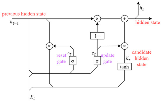
Figure 4. GRU structure diagram.

First, we define the reset gate:

$$r_{\tau }=Sigmoid\left(x_{\tau }+h_{\tau -1}\right)$$

(12)

$$x_{\tau }=\left[\begin{array}{c}{w}_{ijk,month}^{\tau }\\ w_{ijk,week}^{\tau }\\ w_{ijk}^{\tau }\end{array}\right]$$

(13)

where $x_{\tau }$ is the input variable of the time period $\tau$, including the daily average values of travel volume in the time period $\tau$ of the previous month $w_{ijk,month}^{\tau }$, the travel volume in the time period on the same day of the previous week $w_{ijk,week}^{\tau }$, and the travel volume in time period $\tau \left(w_{ijk}^{\tau }\right)$; $h_{\tau -1}$ is the output variable at time $(\tau -1)$, denoted as the previous hidden state. And for the Sigmoid, labeled as $\sigma$ in the figure, it is an S-shaped activation function used to control the flow of features [33].

On this basis, the update gate $z_{\tau }$ is defined as follows:

$$z_{\tau }=Sigmoid\left(x_{\tau }+h_{\tau -1}\right)=W_g{x}_{\tau }+U_g{h}_{\tau -1}$$

(14)

where $W_g$ and $U_g$ are the weight matrices corresponding to $x_{\tau }$ and $h_{\tau -1}$, respectively. The weight matrix changes when the reset gate or update gate performs operations.

Then we define ${\tilde{h}}_{\tau }$ as the flow state generated by the calculation of the input variable $x_{\tau }$ and the output variable at the previous moment $h_{\tau -1}$ in this gate operation, which is calculated as follows:

$${\tilde{h}}_{\tau }=\mathit{tanh}\left(r_{\tau }⨀h_{\tau -1}+x_{\tau }\right)$$

(15)

where tanh is an activation function.

$h_{\tau }$ is defined as the output variable obtained by synthesizing the previous hidden state $h_{\tau -1}$ and the flow state ${\tilde{h}}_{\tau }$ in this gate operation, denoted as the hidden state, which is calculated by the following formula:

$$h_{\tau }=\left(\left(1-z_{\tau }\right)h_{\tau -1}\right)+\left(z_{\tau }⨀{\tilde{h}}_{\tau }\right)$$

(16)

2.

FC Layer

The FC Layer is used to perform linear transformation and non-linear activation on input features, thereby realizing the mapping from the input space to the output space. The linear transformation operation and non-linear activation operation processes of its forward propagation are shown in Formulas (17) and (18), respectively.

$$z=W_l{h}_{\tau }+b$$

(17)

$$y_{\tau }=ReLU\left(z\right)=\mathit{max}\left(0,z\right)$$

(18)

where $h_{\tau }$ is the output variable predicted by the GRU, which serves as the input feature of the FC Layer; $y_{\tau }$ is the output variable of the FC Layer, i.e., the SAV travel volume $w_{ijk}^{\tau }$; $z$ is the intermediate result of linear transformation; $W_l$ is the weight matrix of the FC Layer; $b$ is the bias vector; and $ReLU$ is an activation function [34].

The backpropagation gradient calculation process of the FC Layer is shown in Formulas (19) and (20).

$${\displaystyle \frac{\partial L}{\partial W}}={\displaystyle \frac{\partial L}{\partial z}}{h}_{\tau }$$

(19)

$${\displaystyle \frac{\partial L}{\partial b}}={\displaystyle \frac{\partial L}{\partial z}}$$

(20)

where ${\displaystyle \frac{\partial L}{\partial z}}$ is the gradient of the loss function with respect to the linear transformation result $z$, and $L$ is the loss function.

Formulas (21) and (22) are used to update the weight matrix $W_l$ and the bias vector $b$, where $\alpha$ is the learning rate.

$$W_l=W_l-\alpha {\displaystyle \frac{\partial L}{\partial W_l}}$$

(21)

$$b=b-\alpha {\displaystyle \frac{\partial L}{\partial b}}$$

(22)

3.

Overall Structure of the Model

The FC Layer is used to process the feature information output by the GRU, and the most accurate model weights are fitted through iterative calculations. This part integrates the long-term cumulative effect of the GRU layer, which can effectively improve the accuracy of the model. The overall structure and modeling logic flow of the model are shown in Figure 5 and Figure 6, respectively.

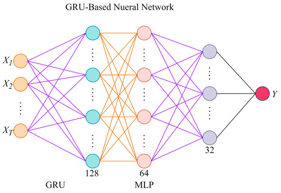
Figure 5. Model structure diagram.

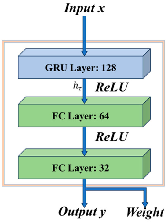
Figure 6. Logic procedure of the model.

The modeling procedure is as follows:

• Input historical data and time series data into the GRU layer, extract 128-dimensional hidden state vectors from each time step, and use the last time step as the input for the subsequent FC layer;
• In the FC layer, the 128-dimensional hidden state vectors output by the GRU layer are used as inputs, which then pass through two FC Layers in sequence to map the hidden state vectors to 32 dimensions, and then serve as the input for the output layer;
• Map the 32-dimensional hidden state vectors processed by the FC layer to a 1-dimensional output $y$, which is $w_{ijk}^{\tau }$.

3.5. Formulation of the System Optimal Model

The benefits and costs of the SAV system primarily encompass three aspects. Specifically, the system revenue refers to the total fees paid by passengers for travel services $R_{travel}$, which reflects the extent to which the system meets passengers’ needs. If the system enhances the supply–demand matching degree through an optimized empty-vehicle relocation strategy, thereby encouraging more people to choose SAV for travel, the system revenue will rise. In terms of costs, it includes the total energy cost incurred by the SAV system for empty-vehicle relocation $C_{Operation}$ and the total maintenance cost for vehicle upkeep $C_{maintenance}$. The calculation methods for each part are as follows:

The value of the total fees paid by passengers for travel services $R_{travel}$ is affected by the number of travel orders completed in time period $t$, i.e., $w_{ijk}^t$, the energy cost for completing one order $c_{ij}$, and the price of one trip $p_{ijk}$. It is calculated using the following formula:

$$R_{travel}=\sum _{t=1}^{\mathbf{T}}\sum _{i\in \mathbf{N}}\sum _{j\in \mathbf{N}\backslash \left\{i\right\}}\sum _{k=1}^{\mathbf{K}}\left(p_{ijk}-c_{ij}\right)w_{ijk}^t$$

(23)

The value of the total energy cost paid by the system for empty-vehicle scheduling $C_{operation}$ is affected by the dispatch volume of SAVs during the operation period $w_{ij0}^t$ and the energy cost consumed by empty driving of vehicles $c_{ij}$. It is calculated using Formula (24):

$$C_{operation}=\sum _{t=1}^{\mathbf{T}}\sum _{i\in \mathbf{N}}\sum _{j\in \mathbf{N}\backslash \left\{i\right\}}{c}_{ij}{w}_{ij0}^t$$

(24)

The value of the total vehicle maintenance cost $C_{maintenance}$ is affected by the total number of SAVs $n_{SAV}$ and the average daily maintenance cost per vehicle $c_m$ (in CNY), as shown in Formula (25):

$$C_{maintenance}=n_{sav}{c}_m$$

(25)

Then, the total profit of the SAV system $P$ can be expressed by Formula (26). The relocation strategy that can achieve the goal of maximizing $P$ is taken as the optimal SAV relocation strategy to be solved in this paper, where the dispatch volume from station $i$ to station $j$ during time period $t$ is the decision variable.

$$\begin{array}{ccc}maxP& =& R_{travel}-C_{operation}-C_{maitenance}\\ & =& \left[{\displaystyle \sum _{t=1}^{\mathbf{T}}}{\displaystyle \sum _{i\in \mathbf{N}}}{\displaystyle \sum _{j\in \mathbf{N}\backslash \left\{i\right\}}}\left({\displaystyle \sum _{k=1}^{\mathbf{K}}}\left(\left(p_{ijk}-c_{ij}\right)w_{ijk}^t\right)-c_{ij}{w}_{ij0}^t\right)-n_{sav}{c}_m\right]\end{array}$$

(26)

Notably, the system optimal model established above, i.e., Formulas (23)–(26), is structured as an integer linear programming model for SAV empty-vehicle dispatching. The core decision variable-hourly empty-vehicle relocation volume $w_{ij0}^t$ is constrained to non-negative integers, as it represents the discrete count of vehicles relocated between districts.

3.6. Solution of the Model

To solve the model, the travel cost matrix between stations must first be calculated, which requires obtaining the inter-station distance matrix $c_{ij}$. By integrating with the urban road network, the Floyd method [35] is employed to compute the shortest path in terms of driving distance along the urban road network, which serves as the distance between each pair of stations $d_{ij}$.

Given that the SAV empty-vehicle scheduling model is an integer linear programming model, the branch and bound algorithm is utilized for its solution [36], as this algorithm is well-suited for finding global optimal solutions to integer linear programming problems and can effectively handle the constraints of vehicle quantity balance and relocation volume limits in our model. For the SAV travel demand prediction model, the Mean Squared Error (MSE) is adopted as the loss function to quantify the discrepancy between the model’s predicted values and the actual values [37].

4. Case Study

4.1. Data Processing

Since SAV is in the trial operation stage in China, there are no actual large-scale SAV operation cases, particularly at the city scale. This paper primarily utilizes city-scale online-hailing taxi data for case studies. The GPS dynamic trajectory data and static basic data of online-hailing taxis are compiled by the Shenzhen Traffic Management Department and taxi GPS platforms [38,39]. Among these, the GPS trajectory data include such items as information collection time, longitude and latitude coordinates, occupancy status, and speed. The data were collected from January to October 2024. After cleaning and processing the original dataset, a total of 1449.6648 billion pieces of data were obtained. The data from January to May 2024 serve as the training dataset for the SAV travel volume prediction model, while the data from June to October function as the test dataset.

After data processing, the travel volume and OD information of each time period are obtained. The total hourly travel volume on a certain day in October 2024 is shown in Figure 7. The data show that the total daily travel volume has an obvious uneven time distribution. Specifically, there is a continuous daytime peak from 8:00 to 17:00, the highest peak of the whole day appears from 20:00 to 23:00, and the lowest peak of the whole day is from 4:00 to 5:00.

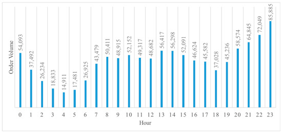
Figure 7. Hourly order volume of the day.

In terms of spatial distribution, the OD distribution among various districts is shown in Figure 8. The results indicate that online-hailing taxi trips are mainly concentrated among Nanshan District, Futian District, and Luohu District. Among them, the average daily OD volumes between Luohu and Futian, and between Nanshan and Futian, reach 349,647 and 171,074, respectively. For the sake of simplified calculation, this paper takes the districts of Shenzhen as traffic zones and uses their centroids as stations.

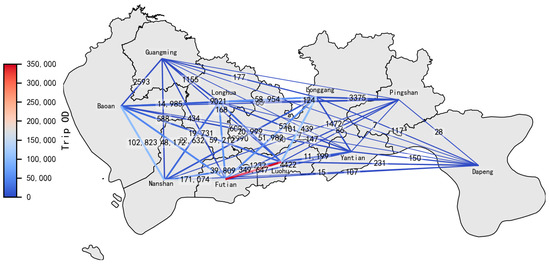
Figure 8. OD distribution of online-hailing taxi trips in Shenzhen.

4.2. Model Solution and Result Analysis

4.2.1. Model Solution

Based on the operation status of online-hailing taxis in Shenzhen [40] and Robo-Taxi in Wuhan and with reference to the actual taxi pricing standards currently implemented in Robo-Taxi in Wuhan, the mileage pricing scheme adopted in this paper are determined and presented in Table 3.

Table 3. Parameter value.

Parameters	Meaning	Values
$∆$	A calculation step	10 min
$l_1$	First-tier mileage for trip pricing	2 km
$l_2$	Second-tier mileage for trip pricing	20 km
$l_3$	Third-tier mileage for trip pricing	20 km
$l_3$	Third-tier mileage for trip pricing	35 km
$p_{{0 \le d}_{ij} \le l_1}$	Rate when the driving mileage is less than $l_1$, i.e., starting rate	10 CNY
$p_{{l_1 \le d}_{ij} \le l_2}$	Rate when the driving mileage is between $l_1$ and $l_2$	2.7 CNY/km
$p_{{l_2 \le d}_{ij} \le l_3}$	Rate when the driving mileage is between $l_2$ and $l_3$	3.51 CNY/km
$p_{d_{ij} \ge l_3}$	Rate when the driving mileage exceeds $l_3$	4.32 CNY/km
$\mu$	Energy cost per unit driving distance	0.175 CNY/km
$c_m$	Average daily maintenance cost of vehicles	16 CNY
${\sigma }_k$	Weight of vehicles with actual passenger load $k$ in the total number of vehicles (excluding relocation trip)	{0.2,0.3,0.4,0.05,0.05}

In addition, the value of energy cost per unit driving distance is derived from the official website of FAW Hongqi [41] and the official website of State Grid e-Charging [42]. By comparing the rated power supply of the vehicle with the maximum driving range, the electricity consumption per 1 km driven by the vehicle is obtained. Multiplying this value by the electricity price data from the official website of State Grid e-Charging, the value is 0.175 CNY/km. The average daily maintenance cost of taxis and the distribution data of actual passenger load are mainly from taxi management companies. On this basis, we assume that the travel volume of passengers participating in ride-sharing with $k=\{1,2,3,4,5\}$ is randomly allocated among each vehicle according to the weight ${\sigma }_k=\{0.2,0.3,0.4,0.05,0.05\}$. In addition, it is assumed that the travel price discount when the number of passengers participating in ride-sharing is $k$, hence ${\rho }_k=\{1.0,0.9,0.8,0.7,0.6\}$.

By adopting the SAV travel volume prediction model and empty-vehicle relocation model proposed in this paper, the hourly empty-vehicle relocation scheme between various districts is implemented. On this basis, results such as the number of relocation times and total system revenue are calculated and compared with the scenario where hourly empty-vehicle relocation is not conducted, so as to demonstrate the applicability and implementation effect of the method proposed in this paper.

4.2.2. Result Analysis

• Results of SAV Travel Prediction

The established deep learning model for SAV travel prediction is trained for 1000 rounds with a learning rate of 0.001, and the training loss function curve is shown in Figure 9. During the 992nd round of training, the value of the model’s loss function is the lowest, with a loss of 0.6924. The model selects the training results of this round as the optimal weight for model verification, and the comparison curve between the prediction results and the original data is shown in Figure 10. Through calculation, generally speaking, the prediction accuracy of SAV travel volume reaches 95.6%, indicating a good prediction effect.

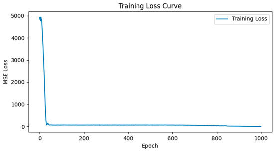
Figure 9. Training loss curve.

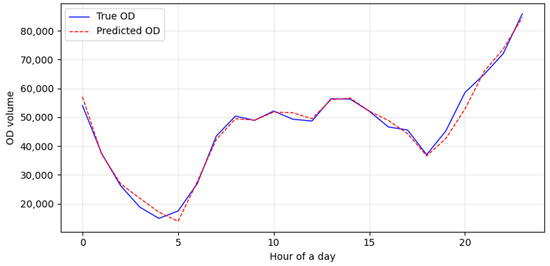
Figure 10. Comparison chart of prediction results and real data.

To further validate the model’s adaptability to SAV operation scenarios where temporal and spatial demand fluctuations are critical, two scenario-specific prediction indicators are supplemented: (1) Peak-hour prediction accuracy: when travel demand surges and directly affects relocation efficiency, the model achieves an accuracy of 93.2% for rush-hour periods (7:00–9:00 and 17:00–19:00). This confirms the GRU-FC model’s ability to capture short-term, high-intensity demand changes—an essential advantage for guiding relocation resource allocation to high-demand areas during peak hours. (2) Spatial prediction accuracy: Evaluated at the 1 km² district level, the model’s accuracy reaches 91.5%. This high spatial precision avoids “blind relocation” to low-demand areas, laying a foundation for improving the utilization of relocated empty vehicles.

2.

Results of System relocation

We take the scenario where there are no hourly system relocations and only natural relocations are relied on as the baseline scheme. Specifically, this means that SAVs travel empty naturally from the destination (drop-off point) of their previous trip to the departure point (pick-up point) of their next trip, without any additional centralized empty-vehicle relocations. The results show that, in the case of the baseline scheme, there are a total of 1,008,559 natural empty-vehicle relocations on average per day, the profit per vehicle is about CNY 357.30/day, and the total system profit is CNY 31,260,891.6/day. After adopting the system scheduling scheme derived from the model in this paper, there are an average of 716,077 natural empty-vehicle relocations and 80,685 system relocations per day. The profit per vehicle is about CNY 496.25/day, and the total system profit is CNY 43,417,905.0/day. The data indicates that, after adopting the system scheduling scheme provided in this paper, both the total system profit and the average profit per vehicle increased by 38.89% compared with those before implementation. The costs and benefits of the two compared schemes are shown in Table 4.

Table 4. Costs and benefits of different schemes.

Schemes	${\mathit{R}}_{\mathit{t}\mathit{r}\mathit{a}\mathit{v}\mathit{e}\mathit{l}}$ (CNY/day)	${\mathit{C}}_{\mathit{o}\mathit{p}\mathit{e}\mathit{r}\mathit{a}\mathit{t}\mathit{i}\mathit{o}\mathit{n}}$ (CNY/day)	${\mathit{C}}_{\mathit{m}\mathit{a}\mathit{i}\mathit{n}\mathit{t}\mathit{e}\mathit{n}\mathit{a}\mathit{n}\mathit{c}\mathit{e}}$ (CNY/day)	Profit (CNY/day)	Profit Per Vehicle-Hour (CNY/Vehicle-Hour)	Demand Fulfillment Rate (%)
Relocation scheme using our model	45,816,018.6	998,241.6	1,399,872.0	43,417,905.0	36.8	88.6
Natural relocation scheme using static algorithm (baseline)	34,119,763.6	1,459,000.0	1,399,872.0	31,260,891.6	26.5	66.5

As shown in Table 4, the proposed scheme achieves a profit per vehicle-hour of CNY 36.8/vehicle-hour—38.9% higher than the baseline’s CNY 26.5/vehicle-hour. This improvement indicates that the system’s resource utilization efficiency is significantly enhanced: under the same operating time, each SAV creates more economic value, which is attributed to the reduction in invalid empty driving and the optimization of relocation paths. Meanwhile, the demand fulfillment rate of the proposed scheme reaches 88.6%, 22.1 percentage points higher than the baseline’s 66.5%—this confirms that system relocations effectively alleviate supply–demand mismatches, ensuring more passenger orders are fulfilled and thus increasing the total travel volume ($R_{travel}$).

There are mainly two reasons for the increase in total system profit. Firstly, the system implements a unified relocation scheme, which reduces natural relocations. Compared with the baseline scheme, the average daily number of natural relocations has decreased by 292,482, accounting for 29.00% of the original daily average. Moreover, when including system relocations, the total number of empty-vehicle relocations in the optimized scheme is 211,797 less than that in the baseline scheme, representing 21.00% of the original daily average of natural relocations. While most of the reduced natural relocations are short-distance trips, and they are replaced by unified cross-district relocations generated by the algorithm, the total relocation cost is still reduced by approximately 32% due to the unified relocations. Moreover, natural relocations from an individual vehicle perspective lack optimization algorithm support and fail to achieve the economic efficiency of system-wide planned relocations. Thus, fewer natural relocations lead to higher profits. Another possible reason is that system relocations reduce passenger flow loss caused by vehicle shortages or excessive passenger waiting times, increasing total travel volume and thereby boosting total system profit. A comparison of the two schemes shows that adopting the relocation scheme proposed in this paper increases the average daily total SAV travel volume by 34.28% compared with the baseline scheme. This is directly reflected in the higher demand fulfillment rate of the proposed scheme (88.6% vs. 66.5% of the baseline) and further translates into a higher $R_{travel}$ (CNY 45.82 million/day vs. CNY 34.12 million/day of the baseline).

The all-day time distribution of natural and system relocation volumes in both schemes is shown in Figure 11. The results indicate that the all-day distribution trend of system relocations is largely consistent with that of SAV travel volumes, but they occur earlier than travel volumes.

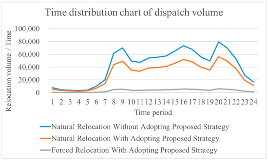
Figure 11. Time distribution of relocation volumes in system and natural schemes.

To clearly illustrate the average daily system relocation OD flows between districts, west-to-east flows are defined as upstream and depicted with blue arrows, while east-to-west flows are defined as downstream and shown with red arrows; the relocation volume of each flow is labeled near the base of the corresponding arrow, as shown in Figure 12. And the results show that the OD pair with the highest empty-vehicle relocation volume is between Futian and Luohu Districts, followed by that between Futian and Nanshan Districts. The total empty-vehicle relocation volume for these two pairs reaches 37,854 per day, accounting for 46.87% of the city’s total daily empty-vehicle relocations.

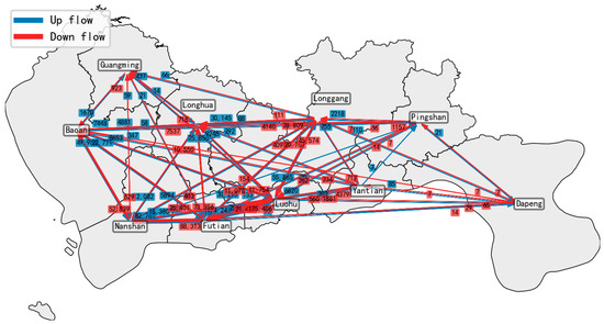
Figure 12. Average daily system relocation OD distribution across districts.

We further calculated the proportions of empty-vehicle relocation origins and destination distribution in each district throughout the day to the total system relocation volume, as shown in Table 5. The results indicate that the top 5 districts with the most empty-vehicle relocation origins are Futian, Luohu, Nanshan, Longgang, and Longhua (in descending order), which are also the top 5 districts with the most empty-vehicle relocation destinations. A high volume of empty-vehicle relocation origins indicates a large number of SAV trips ending in the district, while a high volume of destinations indicates a large number of SAV trips originating from it. Among them, the empty-vehicle relocation destinations in Futian and Luohu are greater than the origins, whereas the opposite is true for other districts. This suggests that, throughout the day, the number of centrifugal SAV trips from these two districts to peripheral areas exceeds that of centripetal SAV trips. However, overall, the all-day directional imbalance in each district is not significant.

Table 5. Proportions of system relocation departures and arrivals in each district to the total volume (%).

Districts	Origin District	Destination District
Luohu	23.46	25.47
Futian	29.66	32.02
Yantian	1.05	0.76
Baoan	9.21	8.63
Guangming	0.34	0.15
Pingshan	0.26	0.12
Longhua	8.49	7.62
Nanshan	15.75	15.6
Dapeng	0.07	0.02
Longgang	11.7	9.62

5. Conclusions

This paper establishes a travel demand-driven dynamic empty-vehicle relocation mechanism for SAVs. By integrating GRU and FC Layers, an SAV travel demand prediction model is developed. On this basis, an integer programming algorithm for SAV empty-vehicle relocation is proposed with the goal of maximizing system benefits, while balancing the interests of both supply and demand sides.

Compared with the baseline natural relocation scheme, the proposed hourly dynamic relocation scheme enhances spatiotemporal supply–demand matching, reducing empty-vehicle relocations and customer loss while increasing total travel volume and system profit. The GRU-FC model effectively captures the time series and spatial characteristics of SAV travel demand, providing reliable support for dynamic relocation decisions. Additionally, the scheme optimizes relocation costs and improves resource utilization efficiency, while raising demand fulfillment rates to balance economic benefits and user experience.

The research enriches the dynamic optimization theory of SAV relocation and provides practical support for “demand-pull”-oriented operational strategies, contributing to improved SAV service quality, reduced empty driving, and coordinated economic and social benefits.

Notably, this paper has certain limitations. Firstly, it does not integrate SAV empty-vehicle relocation with SAV passenger origin–destination and route planning. Future research will focus on two specific directions to address this limitation and further reduce the empty-vehicle rate while improving operational efficiency: (1) incorporating passengers’ OD choice by integrating taxi travel OD prediction modeling with empty-vehicle dispatching and (2) adding a dynamic optimal route decision modeling component to the empty-vehicle dispatching process. Additionally, in the early stage of SAV operation, large-scale urban-level empty-vehicle relocation focuses on increasing time granularity (e.g., the hourly relocation implemented in this paper). In the later stage, other advanced machine learning methods will be explored for SAV travel volume prediction; meanwhile, if computing resources and efficiency permit, spatial computing density can be enhanced by refining district divisions.

6. Discussions

The dynamic scheduling scheme and GRU-FC demand prediction model proposed in this study demonstrate multi-dimensional value in shared autonomous vehicle (SAV) operations. Their effectiveness stems from targeted solutions to the core pain points of traditional static scheduling schemes. From the perspective of operational efficiency, the scheme’s cost optimization effects and higher profit per vehicle-hour benefit from a unified cross-district scheduling mechanism. This mechanism replaces decentralized short-distance natural scheduling which lacks systematic planning. Meanwhile, the concentration of scheduling origin–destination (OD) pairs in core urban areas such as the Futian–Luohu Districts ensures that resources are accurately matched to high-demand areas and avoids blind scheduling.

By addressing the limitations of traditional prediction methods, the GRU-FC model further provides support for the aforementioned scheduling optimization. The model not only achieves excellent overall prediction accuracy but also exhibits advantages in scenario-specific prediction tasks, including high peak-hour prediction accuracy for demand surges during rush hours and refined spatial prediction accuracy for district-level scheduling. These capabilities ensure that scheduling decisions are based on real-time and reliable demand insights. In addition, the significant improvement in demand fulfillment rate directly reduces passenger flow loss caused by insufficient vehicle supply or excessive waiting times. This reflects the scheme’s ability to balance economic benefits such as profit growth and user experience, an aspect that is often overlooked in single-objective optimization studies.

References

- Zhang, C.; Huang, Y.; Ji, A.; Liu, H.; Li, J.; Ni, A.; Lu, W. Policy implications of the transit metropolis project: A quasi-natural experiment from China. Transp. Policy 2025, 162, 155–170. [Google Scholar] [CrossRef]
- Krueger, R.; Rashidi, T.H.; Rose, J.M. Preferences for shared autonomous vehicles. Transp. Res. Part C Emerg. Technol. 2016, 69, 343–355. [Google Scholar] [CrossRef]
- Fagnant, D.J.; Kockelman, K.M. The travel and environmental implications of shared autonomous vehicles, using agent-based model scenarios. Transp. Res. Part C Emerg. Technol. 2014, 40, 1–13. [Google Scholar] [CrossRef]
- Yantao, H.; Kockelman, K.M.; Truong, L.T. SAV operations on a bus line corridor: Travel demand, service frequency, and vehicle size. J. Adv. Transp. 2021, 2021, 5577500. [Google Scholar] [CrossRef]
- Fagnant, D.J.; Kockelman, K.M. Dynamic ride-sharing and fleet sizing for a system of shared autonomous vehicles in Austin, Texas. Transportation 2018, 45, 143–158. [Google Scholar] [CrossRef]
- Zhang, C.; Wu, S.; Huang, M.; Skitmore, M.; Yao, W.; Lu, X. Do carbon emissions trading pilot policies contribute to urban green transportation development? Transp. Res. Part D Transp. Environ. 2025, 140, 104654. [Google Scholar] [CrossRef]
- Li, X.; Zhang, Y.; Yang, Z.; Zhu, Y.; Li, C.; Li, W. Modeling choice behaviors for Ridesplitting under a carbon credit scheme. Sustainability 2023, 15, 12241. [Google Scholar] [CrossRef]
- Li, W.; Li, Y.; Deng, H.; Bao, L. Planning of electric public transport system under battery swap mode. Sustainability 2018, 10, 2528. [Google Scholar] [CrossRef]
- Castaneda, L.J.F.; Toro, E.M.; Gallego, R.R.A. Iterated local search for the vehicle routing problem with a private fleet and a common carrier. Eng. Optim. 2020, 52, 1796–1813. [Google Scholar] [CrossRef]
- Li, W.; Li, Y.; Fan, J.; Deng, H. Siting of carsharing stations based on spatial multi-criteria evaluation: A case study of Shanghai EVCARD. Sustainability 2017, 9, 152. [Google Scholar] [CrossRef]
- Wu, S.; Zou, Y.; Liu, D.; Chen, X.; Wang, Y.; Moeinaddini, A. Investigating Traffic Characteristics at Freeway Merging Areas in Heterogeneous Mixed-Flow Environments. Sustainability 2025, 17, 2282. [Google Scholar] [CrossRef]
- Brendel, A.B.; Lichtenberg, S.; Nastjuk, I.; Kolbe, L.M. Adapting carsharing vehicle relocation strategies for shared autonomous electric vehicle services. In Proceedings of the ICIS 2017 Proceedings, Seoul, Republic of Korea, 10–13 December 2017; Available online: https://aisel.aisnet.org/icis2017/IT-and-Social/Presentations/2 (accessed on 18 November 2025).
- Xu, M.; Meng, Q.; Liu, Z. Electric vehicle fleet size and trip pricing for one-way carsharing services considering vehicle relocation and personnel assignment. Transp. Res. Part B Methodol. 2018, 111, 60–82. [Google Scholar] [CrossRef]
- Overtoom, I.; Correia, G.; Huang, Y.; Verbraeck, A. Assessing the impacts of shared autonomous vehicles on congestion and curb use: A traffic simulation study in The Hague, Netherlands. Int. J. Transp. Sci. Technol. 2020, 9, 195–206. [Google Scholar] [CrossRef]
- Yang, J.; Hu, L.; Jiang, Y. An overnight relocation problem for one-way carsharing systems considering employment planning, return restrictions, and ride sharing of temporary workers. Transp. Res. Part E Logist. Transp. Rev. 2022, 168, 102950. [Google Scholar] [CrossRef]
- Nourinejad, M.; Zhu, S.; Bahrami, S.; Roorda, M.J. Vehicle relocation and staff rebalancing in one-way carsharing systems. Transp. Res. Part E Logist. Transp. Rev. 2015, 81, 98–113. [Google Scholar] [CrossRef]
- Jorge, D.; Molnar, G.; de Almeida Correia, G.H. Trip pricing of one-way station-based carsharing networks with zone and time of day price variations. Transp. Res. Part B Methodol. 2015, 81, 461–482. [Google Scholar] [CrossRef]
- Huang, K.; de Almeida Correia, G.H.; An, K. Solving the station-based one-way carsharing network planning problem with relocations and non-linear demand. Transp. Res. Part C Emerg. Technol. 2018, 90, 1–17. [Google Scholar] [CrossRef]
- Huang, K.; An, K.; de Almeida Correia, G.H. Planning station capacity and fleet size of one-way electric carsharing systems with continuous state of charge functions. Eur. J. Oper. Res. 2020, 287, 1075–1091. [Google Scholar] [CrossRef]
- Kim, S.; Lee, U.; Lee, I.; Kang, N. Idle vehicle relocation strategy through deep learning for shared autonomous electric vehicle system optimization. J. Clean. Prod. 2022, 333, 130055. [Google Scholar] [CrossRef]
- Loo, B.P.Y. Transport, Urban. In International Encyclopedia of Human Geography, 2nd ed.; Elsevier: Amsterdam, The Netherlands, 2020; pp. 457–462. [Google Scholar]
- Jorge, D.; Correia, G.H.A.; Barnhart, C. Comparing optimal relocation operations with simulated relocation policies in one-way carsharing systems. IEEE Trans. Intell. Transp. Syst. 2014, 15, 1667–1675. [Google Scholar] [CrossRef]
- Repoux, M.; Kaspi, M.; Boyacı, B.; Geroliminis, N. Dynamic prediction-based relocation policies in one-way station-based carsharing systems with complete journey reservations. Transp. Res. Part B Methodol. 2019, 130, 82–104. [Google Scholar] [CrossRef]
- Vateekul, P.; Sri-Iesaranusorn, P.; Aiemvaravutigul, P.; Chanakitkarnchok, A.; Rojviboonchai, K. Recurrent Neural-Based Vehicle Demand Forecasting and Relocation Optimization for Car-Sharing System: A Real Use Case in Thailand. J. Adv. Transp. 2021, 2021, 8885671. [Google Scholar] [CrossRef]
- Zhang, S.; Zhang, X.; Shen, L.; Wan, S.; Ren, W. Wavelet-Based Physically Guided Normalization Network for Real-time Traffic Dehazing. Pattern Recognit. 2025, 172, 112451. [Google Scholar] [CrossRef]
- Cartenì, A. The acceptability value of autonomous vehicles: A quantitative analysis of the willingness to pay for shared autonomous vehicles (SAVs) mobility services. Transp. Res. Interdiscip. Perspect. 2020, 8, 100224. [Google Scholar] [CrossRef]
- Zong, F.; Zeng, M.; Yu, P. A parking pricing scheme considering parking dynamics. Transportation 2024, 51, 1349–1371. [Google Scholar] [CrossRef]
- Zong, F.; Zeng, M.; Li, Y.X. Congestion pricing for sustainable urban transportation systems considering carbon emissions and travel habits. Sustain. Cities Soc. 2024, 101, 105198. [Google Scholar] [CrossRef]
- Li, D.; Cao, J.; Li, R.; Wu, L. A spatio-temporal structured LSTM model for short-term prediction of origin-destination matrix in rail transit with multisource data. IEEE Access 2020, 8, 84000–84019. [Google Scholar] [CrossRef]
- Zong, F.; Wu, T.; Jia, H. Taxi drivers’ cruising patterns-Insights from taxi GPS traces. IEEE Trans. Intell. Transp. Syst. 2018, 20, 571–582. [Google Scholar] [CrossRef]
- Lee, E.H.; Kho, S.Y.; Kim, D.K.; Cho, S.H. Travel time prediction using gated recurrent unit and spatio-temporal algorithm. Proc. Inst. Civ. Eng.-Munic. Eng. 2021, 174, 88–96. [Google Scholar] [CrossRef]
- Zhao, H.; Yan, L.; Hou, Z.; Lin, J.; Zhao, Y.; Ji, Z.; Wang, Y. Error Analysis Strategy for Long-Term Correlated Network Systems: Generalized Nonlinear Stochastic Processes and Dual-Layer Filtering Architecture. IEEE Internet Things 2025, 12, 33731–33745. [Google Scholar] [CrossRef]
- Dey, R.; Salem, F.M. Gate-variants of gated recurrent unit (GRU) neural networks. In Proceedings of the 2017 IEEE 60th International Midwest Symposium on Circuits and Systems, Boston, MA, USA, 6–9 August 2017; pp. 1597–1600. [Google Scholar]
- Zong, F.; Zhao, K.; Jiang, S.; Zhang, Z.M. Detecting Highway Pavement Diseases by Developing an Improved YOLOv5 Algorithm. In Proceedings of the International Conference on Artificial Intelligence and Autonomous Transportation, Beijing, China, 6–8 December 2024; Springer Nature: Singapore, 2024; pp. 142–151. [Google Scholar]
- Pešić, D.; Šelmić, M.; Macura, D.; Rosić, M. Finding optimal route by two-criterion Fuzzy Floyd’s algorithm-case study Serbia. Oper. Res. 2020, 20, 119–138. [Google Scholar] [CrossRef]
- Shen, H.; Ding, T.; Mu, C.; Jia, W.; Yuan, Y.; Xue, Y.; Ge, H.; Chang, X.; Li, F. Interval Carbon Emission Flow Model and Bi-Level Branch-and-Bound Algorithm for Power Systems Considering Renewable Energy Uncertainty. Energy 2025, 333, 137344. [Google Scholar] [CrossRef]
- Song, K.; Ma, H.; Zhang, H.; Yan, L. Research of relu output device in ternary optical computer based on parallel fully connected layer. J. Supercomput. 2024, 80, 7269–7292. [Google Scholar] [CrossRef]
- Zhang, D.; Zhao, J.; Zhang, F.; He, T. UrbanCPS: A cyber-physical system based on multi-source big infrastructure data for heterogeneous model integration. In Proceedings of the ACM/IEEE Sixth International Conference on Cyber-Physical Systems, Seattle, WA, USA, 14–16 April 2015; pp. 238–247. [Google Scholar]
- Han, G. Study on the Taxi Operation Monitoring and Decision support Based on Multi-source Data. Traffic Eng. 2020, 20, 62–68. (In Chinese) [Google Scholar]
- Shenzhen Bendibao. Available online: http://sz.bendibao.com/jt/shenzhenchuzuchedongtai/ (accessed on 18 November 2024). (In Chinese).
- Official Website of FAW Hongqi. Available online: https://hongqi.faw.cn/model/E-QM5 (accessed on 13 February 2025). (In Chinese).
- Official Website of State Grid e-Charging. Available online: http://www.evs.sgcc.com.cn/ (accessed on 18 November 2024). (In Chinese).
Disclaimer/Publisher’s Note: The statements, opinions and data contained in all publications are solely those of the individual author(s) and contributor(s) and not of MDPI and/or the editor(s). MDPI and/or the editor(s) disclaim responsibility for any injury to people or property resulting from any ideas, methods, instructions or products referred to in the content. |
© 2026 by the authors. Licensee MDPI, Basel, Switzerland. This article is an open access article distributed under the terms and conditions of the Creative Commons Attribution (CC BY) license.