Abstract
Biodiversity loss is a global environmental concern, mainly driven by human-induced factors, encompassing both direct and indirect drivers. This study investigates the long-term relationship between either the Human Footprint Index (HFI), which measures the extent of human pressures (i.e., direct drivers), or the Gross Domestic Product (GDP), a measure of economic growth (i.e., indirect driver) and biodiversity change, using bird population trends as indicators. The analysis was based on time-series data for Portugal (2004–2023) aggregated at national and sub-national scales, representative of different socio-economic contexts. Multi-species indices were regressed against either the HFI or GDP using Autoregressive Distributed Lag (ARDL) to identify long-run relationships. Bird population trends varied by species group (common, agricultural, and forest birds) and socio-economic context underscoring the importance of sub-national assessments. The HFI and GDP had varying predictive value across species groups and socio-economic contexts, with the HFI showing greater consistency, particularly as a predictor for agricultural birds. While most models showed a negative association between species abundance and either the HFI or GDP, revealing a signal of socio-economic pressures on bird populations at sub-national scales, some models suggested mixed results, indicating that conservation policies must take local contexts into account.
1. Introduction
Human activities and resource use have increased dramatically, especially since the mid-20th century, driven by factors such as population growth, urbanization, and technological advancements [1]. These activities have led to widespread changes observed globally, with Earth’s landscapes and systems being drastically transformed [1,2]. As a result, biodiversity change and loss have emerged among the most critical environmental challenges we face today [3].
In addition to the ethical questions, the decline in biodiversity might ultimately result in ecosystems losing their capacity to deliver ecosystem services and, thus, threaten human well-being [3,4,5,6]. Ecosystem services are “the contributions that ecosystems make to human well-being” [7], and are classified into three main categories: provisioning services (such as food or clean water), regulating services (such as climate regulation or disease regulation), or cultural services (for spiritual, aesthetic, or recreational purposes) [7]. Land use change, including habitat conversion for resource extraction—particularly for provisioning services [8,9]—along with habitat degradation and fragmentation, often leads to environmental degradation and biodiversity loss, undermining the maintenance of regulation and cultural ecosystem services [5,8,9,10].
Pressures, such as those measured by the Human Footprint Index (HFI), directly impact ecosystems and act as the direct drivers of biodiversity change (i.e., factors that operate directly on nature and are the immediate cause of biodiversity change [5]). The HFI, introduced by Sanderson et al. [11] in the early 2000s, combines multiple pressures into a single metric, making it a valuable tool for assessing and tracking human influence on ecosystems. The HFI generates a cumulative threat map that measures both the extent and intensity of human impact on ecosystems across the entire planet. Over the years, the HFI has been calculated in different ways, incorporating increasingly dynamic datasets as technology advances [12]. It is composed of eight variables that function as proxies of both direct and indirect human pressures: (1) built environments, (2) population density, (3) electric infrastructure, (4) croplands, (5) pasture lands, (6) roads, (7) railways, and (8) navigable waterways [13]. Each variable contributes differently to the index, as they have distinct characteristics that affect how their pressure is captured [13].
The trends in these direct drivers are ultimately shaped by indirect drivers, such as economic growth or governance systems [5]. Economic growth, in particular, is a key factor influencing the trends in direct pressures [5,10]. Economic growth refers to the increase in the production of goods and services in an economy over a period of time [10], and it is typically quantified by the Gross Domestic Product (GDP). GDP is often viewed as a proxy indicator of a nation’s prosperity and is associated with improvements in human well-being, despite its shortcomings for the purpose [14].
Ecosystem services provide the essential inputs for economic development [9]. However, while benefiting from these services, economic activities often put significant pressures on ecosystems and natural resources, eventually leading to their depletion and potentially resulting in both environmental and economic collapse [15]. Therefore, there might be a conflict between preserving biodiversity and pursuing economic growth [10].
The impact of economic growth on biodiversity has predominantly been assessed at supranational scales, often yielding inconclusive results. However, most studies indicate a negative relationship between economic prosperity and biodiversity conservation, with potential implications for long-term sustainability [16,17].
In response to these concerns, the concept of Degrowth argues that economic growth should neither be viewed as a goal nor a necessity. Instead, it defends that societies should deliberately reduce production and consumption, leading to a lower GDP [18,19]. Conversely, proponents of Decoupling, or Green Growth, argue that economic growth can and should be pursued without increasing natural resource consumption, waste, or emissions [20,21]. They suggest that greater financial capacity, combined with technological advancements, can drive investment in conservation and promote more sustainable practices, allowing economic growth to coexist with biodiversity conservation [17,22,23].
Given these contrasting theoretical frameworks and the inherently localized nature of biodiversity impacts, it is important to understand how biodiversity responds at more localized scales, where decisions on ecosystem use are implemented. Moreover, it is important to understand whether these responses are consistent across different socio-economic contexts for informing effective conservation strategies.
Here, we aim to assess and compare the long-term response of biodiversity to direct human pressures and to economic growth at national and sub-national scales in continental Portugal. Specifically, we investigate how the HFI, as an indicator of direct pressures, and GDP, as an indicator of economic growth, influence trends in bird population abundance. We also compare the predictive capacity of these indicators at sub-national scales and assess whether their effects differ across varying socio-economic contexts. We use bird census data to calculate multi-species indices as these are regarded as good biodiversity indicators due to their responsiveness to change, timeliness, and scalability, and also due to the availability of long-term data [24,25,26].
2. Materials and Methods
2.1. Study Design and Multi-Scale Approach
A multi-scale approach was implemented to investigate the response of bird population abundance to the HFI and GDP at both national and sub-national scales. Specifically, bird population abundance data collected between 2004 and 2023 in 10 km × 10 km grid cells (hereafter, bird data cells—Appendix A) (see Section 2.2) were used to estimate yearly abundance indices that were regressed against time-series data of the HFI and GDP (see Section 2.3). This analysis was conducted at the national scale, using all 170 bird data cells available from the Common Birds Census (CAC), provided by the Portuguese Society for the Study of Birds (SPEA), for continental Portugal, and at the sub-national scale, employing two clustering approaches (Figure 1 and Figure 2).
Figure 1.
Bird data cells’ cluster categories for the HFI (left) and GDP (right).
Figure 2.
Methodology scheme for national and sub-national analysis.
In the first sub-national clustering approach, bird data cells were classified and grouped based on their 2020 HFI values into three categories: low, medium, and high HFI. In the second sub-national clustering approach, bird data cells were grouped according to the GDP levels of the corresponding NUTS III regions (the highest resolution available) in 2020, and were categorized into low, medium, and high GDP categories. The HFI was chosen for its ability to combine various direct human pressures, providing a measure of human impact on ecosystems, while GDP was selected because it is a widely recognized measure of economic growth. By clustering based on the HFI and GDP, we adopted a stratified approach that captured different socio-economic contexts—one reflecting the degree of landscape transformation and the other the economic scale.
The thresholds defining the limits of each cluster category were determined using the Jenks Natural Breaks method, which maximizes the variance between classes and minimizes the variance within classes [27]. Subsequently, minor adjustments were made to ensure a balanced distribution of bird data cells across clusters. For the first sub-national clustering approach, 30 bird data cells were included in the “high HFI” cluster, 50 in the “medium HFI” cluster, and 90 in the “low HFI” cluster. For the second sub-national clustering approach, 28 bird data cells comprised the “high GDP” cluster, 47 the “medium GDP” cluster, and 95 the “low GDP” cluster. The resulting division of bird data cells for the two approaches is shown in Figure 1. We acknowledge that clustering thresholds can influence group configurations and, consequently, the results. Preliminary testing showed that, in this case, alternative thresholds led to highly unbalanced cluster sizes, compromising statistical robustness and group comparability. Therefore, we did not pursue alternative thresholds or conduct sensitivity analyses. This represents a limitation that should be considered when interpreting the findings of this study.
At both the national scale and within each cluster, multi-species indices for common, agricultural, and forest birds (Appendix B) were computed (see Section 2.4) and used as dependent variables in time-series models, with either the HFI or GDP as the independent variables (see Section 2.5). Although GDP and the HFI are related, as economic activity often comes at the cost of human pressures on the environment [10], they represent distinct dimensions of socio-economic dynamics and were therefore analyzed as independent variables separately. Additionally, their time series were not significantly correlated (p-value > 0.05) in any of the cases.
2.2. Bird Species Data
Throughout this study, population abundance trends of common birds resident in continental Portugal were employed as indicators of biodiversity change. To develop these indicators, we utilized data from the CAC, provided by SPEA, covering a 20-year period from 2004 to 2023 [28]. The CAC is a bird monitoring program conducted by volunteers and comprises of data on 65 different species of common birds in continental Portugal. The sampling unit is the 10 km × 10 km UTM (Universal Transverse Mercator coordinate system) grid square. Alonso et al. [28] details the methodology employed in data collection.
In total, available data account for 170 bird data cells (Figure 1) distributed throughout the country. Appendix A contains the UTM codes of each bird data cell, the total number of visits between 2004 and 2023, and other relevant information.
2.3. Anthropogenic Data
The HFI variable was derived from two complementary datasets. Cell clustering, based on 2020 data, was performed using the dataset with finer spatial resolution (300 m, 2000–2020 [12]), while the time series was extracted from Mu et al. [29], which provided a longer temporal coverage (2000–2022), allowing for a consistent time series from 2004 to 2022 (Appendix C, Figure A1). HFI values for each bird data cell for each year were extracted from ArcGIS Pro (version 3.1.41833) by calculating the average value within that area.
Portuguese national GDP was obtained from AMECO database [30] (Appendix C, Figure A2), while the NUTS III dataset (the highest resolution available), used in the sub-national analyses, was obtained from Statistics Portugal [31]. We have employed the GDP deflator available in AMECO (base year 2015 (This is the base year provided in the AMECO national-scale GDP deflator and was adopted, for consistency, for the NUTS III regional data as well)) to convert both national and regional GDP data from nominal to real values. For each NUTS III region and at the national level, nominal GDP was divided by the national-level AMECO GDP deflator and multiplied by 100 to give real GDP. The lack of data availability for region-specific GDP deflators and the limited price and inflation variation between regions in the same country make this a pragmatic and consistent approach to conducting our work using comparable national and regional GDP datasets in real value.
2.4. Estimation of Species Population Trends
In line with Alonso et al. [28], the 65 studied species, all considered “common” species (i.e., abundant and widespread species), were divided and categorized as one of three habitat categories—“agricultural” (23 species), “forest” (19 species), and “other” (23 species)—as presented in Appendix B. Along with the individual species indices, multi-species indices were also calculated for common, agricultural, and forest categories. Since the “other species” category includes a wide variety of species that inhabit diverse habitat types, they were not analyzed as a single group.
Annual changes in bird population abundance were estimated using the abundance values gathered for each species, per year and per bird data cell. The annual indices took the first year of study, 2004, as the baseline, assigning it a value of 1. Subsequent annual indices were calculated based on the 2004 value.
Indices were calculated in R 4.3.2 software, using TRends & Indices for Monitoring data (TRIM) (rtrim 2.1.1 package) [32] for individual indices, and the Multi-Species Indicator Tool (MSI) (adaptations from the MSI 3.1 script) [33] for the multi-species indices.
In this work, both Models 2 and 3 from rtrim package were used. Model 2 considers the site effects for each location and adds a linear time effect. Model 3 incorporates both site effects for each location and time effects for each year [32,34]. Since Model 3 considers that the species counts differ between places, it was used when analyzing on a large, national scale. However, when downsizing to a sub-national scale, there was insufficient data for applying Model 3, so Model 2 was used instead. The models’ outputs for each species consisted of a population index for every year of the study and its associated standard error.
Then, the MSI used individual species’ annual indices and their corresponding standard errors to calculate the multi-species annual indices for a specific group, along with their confidence intervals [33]. They are projected using Monte Carlo simulations, where each annual index for each species is simulated 1000 times by sampling from a normal distribution , where is the natural logarithm of the index and is the standard error on the log scale [33]. After each simulation, the geometric mean and the standard error of the simulated species indices are used to compute the multi-species indices and confidence intervals for each year, using the Delta method [33]. Then, they are back-transformed to the index scale [33]. In addition to calculating annual indices for each group as percentages, the MSI also estimates linear and smooth trends using Monte Carlo simulations based on confidence intervals and limits. These trends are not only used for visual representations but also to classify the indices into categories such as “uncertain”, “stable”, “strong increase”, “moderate increase”, “steep decline”, or “moderate decline”, according to Soldaat et al. [33] (Table 1).
Table 1.
MSI trend classification [33] (CI = confidence interval; CL = confidence limit).
2.5. Time Series Correlation Analysis
After obtaining multi-species indices that represent the birds’ population trends at the national and sub-national levels, these time series were used as dependent variables and regressed against either the HFI or GDP (independent variables). The goal was to investigate the existence of a long-term effect of the HFI or GDP on species population abundance.
Time series analysis was conducted using the software EViews 12 SV. To test the presence of significant long-run relationships between the variables, we utilized Autoregressive Distributed Lag (ARDL) models, motivated by the small sample size and mixed order of integration for our variables [35,36]. To ensure that the ARDL Bounds test for cointegration was valid and avoid the risk of spurious regression, we conducted unit root tests to verify that all the time series were at most a first-order integrated process—I(1).
In our analysis, we estimated ARDL models including a restricted constant and no trend, which is the standard (Case II in EViews), and suitable when the variables have different levels but do not exhibit systematic trends [36]. The lag length assigned to each variable was selected based on the Akaike Information Criterion [37], after setting a maximum lag length of four. The residuals of ARDL models were tested to ensure no trace of serial correlation or heteroskedasticity.
The Bounds test then determined whether a long-run relationship (cointegration) existed between variables [36]. For two variables (dependent Y and independent X), the general ARDL model is:
On the l.h.s. of Equation (1) is the change in the dependent variable and on the r.h.s. are, respectively, a constant , the short-run dynamics of Y, the short-run dynamics of X, the long-run relationship between the two, and an error term . The Bounds test examines whether the long-run coefficients are jointly zero () (null hypothesis). If this hypothesis is rejected, then there is evidence for a long-run cointegration relationship linking the dependent and independent variables. This is performed by comparing the Wald test F-statistic against the Pesaran critical values [36] at the 5% and 1% significance levels.
If the Bounds test leads to the conclusion of cointegration, the long-run relationship between the variables can be meaningfully estimated as:
With , , and . The coefficient communicates the long-term effect of the independent variable (HFI or GDP) on the dependent variable (multi-species population indices), e.g., if the coefficient associated with GDP is negative and significant, it strongly suggests that the multi-species index is negatively affected as GDP increases. It is important to note that these coefficients are tied to the units of their respective variables, so they may have different orders of magnitude, depending on whether they are associated with the HFI or GDP.
Although for long-run cointegration analysis the Bounds test results and the significance of the error-correction term and long-run coefficients are of primary importance, each model’s goodness of fit is evaluated by also observing the R-squared metric.
3. Results
3.1. Bird Population Trends
Bird population trends, between 2004 and 2023, varied across spatial scales, socio-economic contexts, and species groups (Figure 3).
Figure 3.
Population trends of common (left), agricultural (middle), and forest (right) birds for each conducted approach—national (first row), sub-national HFI clusters (second row), sub-national GDP clusters (third row)—in the period between 2004 and 2023. The graphics in the first row, the national approach, use the same data as those in Alonso et al. [28].
At the national level, and according to the MSI classification system (Table 1), common bird species have maintained a stable trend over the past 20 years. Contrastingly, agricultural bird populations have experienced a moderate decline, while forest birds have shown a moderate increase during the same period.
The indices calculated by HFI clusters, which represent different levels of human direct pressures and landscape transformation, reveal that in areas with high HFI values, common birds exhibited stable trends, as well as agricultural birds, whereas forest birds experienced a moderate decline. In regions with medium HFI values, all three groups—common, agricultural, and forest birds—had moderate increases. Finally, in areas with low HFI values, common birds and agricultural birds had a moderate decline, and forest birds had a moderate increase.
Regarding GDP clusters, which represent different levels of economic activity, results show that in high GDP zones, common and forest birds experienced a moderate increase, while agricultural birds remained stable. In areas with medium GDP values, population trends for agricultural and forest birds were stable, while common birds experienced a moderate increase. In low GDP zones, common and agricultural birds experienced a moderate decline, and forest species had a moderate increase.
3.2. Long-Run Relationship Between the Population Trends, HFI, and GDP
ARDL models were used to regress population trends against either the HFI or GDP and Bounds tests were conducted to assess the presence of a long-run relationship between the variables. Table 2 presents the results of these tests, along with the coefficients and R-squared values of the significant models.
Table 2.
Results for national and sub-national approaches. The MSI classification (↔—stable; ↑—moderate increase; ↓—moderate decline) is indicated per bird group and scale of analysis. Coefficients and R-squared values are presented for the ARDL models (ns—not significant).
On the national scale, only two models demonstrated a significant long-run relationship. Specifically, agricultural birds responded to the HFI, while common bird populations responded to GDP. Both models exhibited negative coefficients, indicating that increases in the HFI and GDP are associated with declines in the national agricultural bird index and common bird index, respectively.
When regressing the bird indices for each HFI cluster with the HFI as independent variable, a significant long-run relationship was found in most cases (seven out of nine), except for agricultural birds in medium HFI zones and common birds in low HFI zones. In areas with a medium HFI, the associated coefficient was positive for common and forest birds, as was the case for forest birds in zones with a low HFI. Conversely, the coefficient was negative in the remaining cases.
When GDP was the independent variable, using the same clusters, a long-run relationship was found for five out of nine models: for common and agricultural birds in high HFI areas, for common and forest birds in medium HFI areas, and for agricultural birds in low HFI areas. Most models presented a negative coefficient associated with GDP, except for common birds in medium HFI areas, which showed a positive coefficient.
When clustering the bird data cells by GDP levels, and using the HFI as the independent variable, five out of nine models demonstrated significant long-run relationships: agricultural birds in all three GDP levels and common birds in medium and low GDP areas. The associated coefficients were negative in all cases, except for common birds in medium GDP zones, which presented a positive response to the HFI in the long-run.
Using the same bird data cell clustering, but with GDP as the independent variable, most long-run relationships were not significant, except for agricultural and forest birds in high GDP zones and for agricultural birds in medium GDP zones (three out of nine models). Among the models with significant results, all were associated with negative coefficients for GDP.
4. Discussion
4.1. Bird Population Trends at National and Sub-National Levels
Bird population trends varied by spatial scale, socio-economic context, and species groups (Figure 3, Table 2). This finding points to the need for a better understanding of scale effects on aggregated trends and for refining assessment scales to better align available data with policy needs [38]. Moreover, while multi-species indices reveal only moderate changes or stable trends at the species group level, some individual species exhibited strong declines or increases (see Appendix B). For declining species, these patterns may justify and call for targeted conservation approaches [39]. Furthermore, because the base year for the study was 2004, the observed trends pertain only to that time interval and may not be representative of longer-term patterns. For example, increasing trends could reflect recovery trajectories that may not yet be sufficient to compensate for or exceed past losses.
At the national level, agricultural birds have experienced a moderate decline over the past 20 years, while forest birds showed a moderate increase, leading to a stable trend for the overall common birds. Similar trends have been reported for Europe. Rigal et al. [40] reported declines in both agricultural and forest bird species, with agricultural birds declining more sharply. In the same study, however, and in line with national results, forest species showed positive trends in Portugal. Gregory et al. [41,42] confirmed declines in agricultural birds, with stable or rising populations of forest birds, a pattern also noted by Burns et al. [26] for Mediterranean forests. The decline in agricultural bird populations in Europe is often attributed to two distinct drivers: agricultural intensification and agricultural abandonment [40,43,44], though numerous other factors may also contribute. This latter phenomenon might also contribute to explaining the increasing trends in forest birds across Europe. As agricultural areas are left uncultivated, natural vegetation can regrow, leading to habitat recovery that benefits forest species [40,43].
At the sub-national scale, agricultural bird populations increased in areas with a medium HFI, declined in areas with a low HFI or GDP, and remained stable in areas with a high HFI and GDP or medium GDP (Figure 3, Table 2). Forest birds, on the other hand, increased in areas of low and medium HFI and of high and low GDP, decreased in areas of high HFI, and remained stable in areas with medium GDP (Figure 3, Table 2).
The contrasting trends of forest birds in areas of high HFI, where a declining trend is observed, and in areas of high GDP, where an increasing trend is observed, could be explained by the features of bird data cells included in these clusters (Figure 1). Although similar population trends might be expected across the two clusters, the high HFI cluster is circumscribed to areas with high urban densification and infrastructure, such as the coastal areas near Lisbon and some cells in the Algarve region. In contrast, the high GDP cluster includes peri-urban and natural areas in the Metropolitan Area of Lisbon, while excluding areas experiencing high human pressures—despite lacking a strong economic profile, like the bird data cells in the Algarve region. These contrasting results highlight the importance of assessing biodiversity responses to pressures and drivers at relevant scales.
Moreover, the distinct abundance trends observed in each cluster indicate that national scale analyses cannot fully capture the nuanced trends present at sub-national levels, underscoring the importance of considering smaller scales in assessment and policy.
4.2. Long-Term Response of Biodiversity to Economic Growth and Human Activity
Significant long-term associations were found, either with the HFI or GDP, for most species groups and tested scales (Table 2). Three main patterns emerge. First, the stratification of bird data cells based on HFI values yielded more significant models than the stratification based on GDP. Second, and relatedly, models using the HFI as the independent predictor yielded more significant long-run relationships and generally higher R-squared values compared to those using GDP as the predictor. Both findings suggest that the HFI may be a suitable predictor of bird population changes at sub-national scales and over large time intervals. This can likely be attributed to the HFI’s composition, as it incorporates multiple factors that directly influence ecosystems, such as urbanization and infrastructure development. The limited explanatory power of GDP, as found for this study and others (e.g., Kerr and Currie [45] for birds, Mozumder et al. [46] and Mikkelson et al. [47]), may reflect its indirect relationship with biodiversity, as economic growth does not uniformly translate into either positive or negative outcomes for ecosystems. On the other hand, as discussed below, a longer temporal window may be needed to detect the full effects of GDP on biodiversity. Third, more long-run relationships were found for agricultural birds than forest birds (Table 2). While forest birds mostly responded to the HFI in HFI clusters, agricultural birds also responded to the HFI in GDP clusters. A possible explanation, but requiring further testing, relates to the fact that agricultural birds are more connected to human land uses and economic activities, particularly farming, and therefore, GDP clustering may be useful to capture different types of responses to drivers of change. In contrast, forest birds may be more dependent on natural and semi-natural habitats, and more sensitive to direct human pressures, which are better captured by HFI clustering.
Regarding the models’ coefficients, which indicate the direction of the relationship between bird population trends and HFI and GDP trends, most models showed negative coefficients, indicating a detrimental long-term effect of the tested drivers on bird population abundance. Exceptions were found for common birds in areas of medium HFI and medium GDP, and for forest birds in areas of medium and low HFI, which demonstrated a positive coefficient. Additionally, note that in the regression models between forest bird population trends and GDP time series in areas with a medium HFI and high GDP, the coefficients were negative, which is inconsistent with the increasing trends observed for forest birds in the two clusters. These discrepancies may stem from the idiosyncratic nature of the GDP time series between 2004 and 2023 (Appendix C), which includes periods of economic recession, such as the financial crises between 2010 and 2014, as well as the global COVID-19 pandemic in 2020. These short-term events could have led to model overfitting, masking long-term trends. Therefore, a longer temporal window may be necessary to detect and confirm the full effects of GDP on these species’ groups.
At the national level, only two models showed significant long-run relationships: agricultural birds with the HFI and common birds with GDP, both of which had negative coefficients. At the sub-national levels, most of the significant long-run models also displayed negative coefficients for the independent variables. In those cases, the effects of either the HFI or GDP on bird species population abundance appear to be negative. This aligns with studies that suggest a conflict between economic growth and biodiversity conservation [16,17].
On the other hand, common birds in medium HFI zones responded positively to both the HFI and GDP, and in medium GDP zones responded positively to the HFI, while forest birds in medium and low HFI zones responded positively to the HFI. Both groups exhibited increasing trends at the respective clusters, suggesting that these species may be recovering in these areas due to specific changes in ecosystem use and management, such as agricultural abandonment, as previously mentioned. While not in the scope of the present study, we acknowledge the need for further investigation into individualized drivers to better understand the specific factors shaping these species trends. Overall, these results could support the possibility of Decoupling [20,21], which suggests that economic development and biodiversity conservation can, under certain conditions, progress independently of one another, with opportunities for biodiversity recovery and enhancement. Moreover, although there may be issues with the relationship found in these model (see above), the increase in forest bird populations in high GDP zones (Figure 3) is worth noting. The underlying mechanisms of these trends require dedicated research; however, a possible explanation could be the increased availability of forested habitats in the areas of both medium HFI and high GDP. This could be attributed to a higher availability of urban green spaces, such as parks and gardens, as well as abandoned farming parcels in peri-urban agricultural lands.
Finally, it is important to note that a positive or negative coefficient does not necessarily imply a causal relationship between variables. Significant associations between the HFI or GDP and bird population trends do not automatically indicate that these factors directly drive changes in bird populations. In this study, we focused on two independent variables—HFI and GDP—to assess their impact on bird population abundance. However, individualized factors within the HFI or other underlying factors not considered in our models may have contributed to the observed patterns.
5. Conclusions
The objective of this study was to examine the existence of long-term effects of the HFI and GDP on bird population trends and to assess whether these relationships are consistent across different socio-economic contexts at the sub-national scale. Results revealed diverse population trends, varying by species group and socio-economic context, highlighting the importance of recognizing the diversity of species responses to human-induced drivers and considering socio-economic clusters that capture local nuances while still reflecting broader patterns relevant to inform policy.
Results also suggest that the stratification by socio-economic clusters allows for the detection of context-specific responses of bird populations to socio-economic drivers. In this study, the response to direct pressures, represented by the HFI, was found to be potentially stronger than the response to indirect drivers, represented by GDP. Moreover, the majority of the significant long-run relationships suggested a negative response of species abundance to the HFI or GDP, confirming a detrimental impact of human-induced pressures and economic growth on biodiversity. However, a few models also revealed positive associations, indicating that in some contexts, species may show recovery of increasing trends in tandem with landscape transformation and economic growth. It is also important to note that, while birds are widely used as indicators of biodiversity due to their ecological responsiveness and data availability, the patterns observed in bird populations may not fully capture trends in other taxonomic groups, representing a limitation of this study. While still exploratory, the findings of this study provide a valuable foundation for more comprehensive research on the relationship between socio-economic drivers and biodiversity across diverse socio-economic contexts.
Author Contributions
Conceptualization, L.B. and V.P.; methodology, L.B., V.P., J.S. and T.D.; software, L.B.; formal analysis, L.B.; resources, L.B. and V.P.; writing—original draft preparation, L.B.; writing—review and editing, L.B., V.P., J.S. and T.D.; supervision, V.P., J.S. and T.D. All authors have read and agreed to the published version of the manuscript.
Funding
Financial support for this research was provided by FCT/MCTES (PIDDAC) through projects LARSyS-FCT Pluriannual funding (UIDB/50009/2025, UIDP/50009/2025, and LA/P/0083/2020), and https://doi.org/10.54499/CEECIND/04469/2017/CP1461/CT0023 (V. Proença). This work was also supported by MAPS—Models, Assessment, and Policies for Sustainability (Horizon Europe, grant
agreement Nº 101137914) and by Project Blockchain. PT—Decentralize Portugalwith Blockchain Agenda (Project no. 51), Call no 02/C05-i01.01/2022, funded by the Portuguese Recovery and Resilience Program (PRR), the Portuguese Republic, and the European Union (EU) under the framework of the Next Generation EU Program.
Institutional Review Board Statement
Not applicable.
Informed Consent Statement
Not applicable.
Data Availability Statement
Restrictions apply to the availability of bird census data, which were obtained from the Portuguese Society for the Study of Birds (SPEA) and may be available upon request.
Acknowledgments
The authors thank SPEA for the data provided from the Common Birds Census.
Conflicts of Interest
The authors declare no conflicts of interest.
Abbreviations
The following abbreviations are used in this manuscript:
| ARDL | Autoregressive Distributed Lag |
| CAC | Common Birds Census |
| GDP | Gross Domestic Product |
| HFI | Human Footprint Index |
| MSI-Tool | Multi-Species Indicator Tool |
| SPEA | Portuguese Society for the Study of Birds |
| TRIM | TRends & Indices for Monitoring data |
| UTM | Universal Transverse Mercator coordinate system |
Appendix A. Bird Data Cell Information
Table A1.
Bird data cell information.
Table A1.
Bird data cell information.
| Bird Data Cell | UTM | NUTSII | Nº of Visits | HFI Category | GDP Category |
|---|---|---|---|---|---|
| 1 | MC68 | Lisboa | 12 | High | High |
| 2 | MC69 | Lisboa | 15 | High | High |
| 3 | MC78 | Lisboa | 10 | High | High |
| 4 | MC85 | Lisboa | 4 | Medium | High |
| 5 | MC86 | Lisboa | 4 | Medium | High |
| 6 | MC87 | Lisboa | 5 | High | High |
| 7 | MC95 | Lisboa | 15 | Medium | High |
| 8 | MC97 | Lisboa | 9 | High | High |
| 9 | MD60 | Lisboa | 7 | Medium | High |
| 10 | MD61 | Lisboa | 3 | High | High |
| 11 | MD70 | Lisboa | 4 | Medium | High |
| 12 | MD71 | Lisboa | 5 | Medium | High |
| 13 | MD72 | Centro | 5 | High | Medium |
| 14 | MD73 | Centro | 6 | Medium | Medium |
| 15 | MD74 | Centro | 7 | High | Medium |
| 16 | MD75 | Centro | 5 | Medium | Medium |
| 17 | MD80 | Lisboa | 6 | Medium | High |
| 18 | MD81 | Centro | 11 | Medium | Medium |
| 19 | MD82 | Centro | 5 | Medium | Medium |
| 20 | MD84 | Centro | 1 | Medium | Medium |
| 21 | MD90 | Lisboa | 9 | High | High |
| 22 | MD91 | Centro | 5 | Medium | Medium |
| 23 | MD98 | Centro | 7 | Medium | Medium |
| 24 | NB10 | Algarve | 7 | Low | Medium |
| 25 | NB19 | Alentejo | 6 | Medium | Low |
| 26 | NB31 | Algarve | 20 | Medium | Medium |
| 27 | NB35 | Alentejo | 6 | Low | Low |
| 28 | NB41 | Algarve | 3 | Medium | Medium |
| 29 | NB56 | Alentejo | 15 | Low | Low |
| 30 | NB61 | Algarve | 2 | Medium | Medium |
| 31 | NB68 | Alentejo | 10 | Low | Low |
| 32 | NB69 | Alentejo | 4 | Low | Low |
| 33 | NB70 | Algarve | 7 | High | Medium |
| 34 | NB72 | Algarve | 3 | Low | Medium |
| 35 | NB80 | Algarve | 1 | High | Medium |
| 36 | NB82 | Algarve | 5 | Low | Medium |
| 37 | NB83 | Alentejo | 2 | Low | Low |
| 38 | NB90 | Algarve | 11 | High | Medium |
| 39 | NB94 | Alentejo | 2 | Low | Low |
| 40 | NC06 | Lisboa | 14 | Medium | High |
| 41 | NC08 | Lisboa | 2 | High | High |
| 42 | NC16 | Lisboa | 5 | High | High |
| 43 | NC18 | Lisboa | 3 | Low | High |
| 44 | NC21 | Alentejo | 3 | Low | Low |
| 45 | NC23 | Alentejo | 9 | Low | Low |
| 46 | NC25 | Alentejo | 1 | Low | Low |
| 47 | NC30 | Alentejo | 19 | Low | Low |
| 48 | NC35 | Alentejo | 19 | Low | Low |
| 49 | NC41 | Alentejo | 11 | Low | Low |
| 50 | NC43 | Alentejo | 1 | Low | Low |
| 51 | NC56 | Alentejo | 9 | Low | Low |
| 52 | NC59 | Alentejo | 14 | Low | Low |
| 53 | NC69 | Alentejo | 3 | Low | Low |
| 54 | NC73 | Alentejo | 1 | Low | Low |
| 55 | NC75 | Alentejo | 3 | Low | Low |
| 56 | NC76 | Alentejo | 7 | Low | Low |
| 57 | NC82 | Alentejo | 8 | Low | Low |
| 58 | NC83 | Alentejo | 1 | Low | Low |
| 59 | ND00 | Lisboa | 5 | Medium | High |
| 60 | ND01 | Lisboa | 6 | High | High |
| 61 | ND07 | Centro | 20 | Medium | Medium |
| 62 | ND11 | Alentejo | 14 | Medium | Low |
| 63 | ND12 | Alentejo | 11 | Medium | Low |
| 64 | ND13 | Alentejo | 14 | Medium | Low |
| 65 | ND14 | Alentejo | 8 | Medium | Low |
| 66 | ND15 | Alentejo | 1 | Low | Low |
| 67 | ND17 | Centro | 9 | Low | Medium |
| 68 | ND18 | Centro | 7 | Medium | Medium |
| 69 | ND21 | Alentejo | 9 | Low | Low |
| 70 | ND22 | Alentejo | 4 | Medium | Low |
| 71 | ND23 | Alentejo | 1 | Medium | Low |
| 72 | ND24 | Alentejo | 20 | High | Low |
| 73 | ND25 | Alentejo | 12 | Medium | Low |
| 74 | ND26 | Centro | 5 | Medium | Low |
| 75 | ND32 | Alentejo | 1 | Low | Low |
| 76 | ND35 | Alentejo | 8 | Medium | Low |
| 77 | ND40 | Alentejo | 20 | Low | Low |
| 78 | ND41 | Alentejo | 1 | Low | Low |
| 79 | ND44 | Alentejo | 15 | Low | Low |
| 80 | ND45 | Alentejo | 8 | Low | Low |
| 81 | ND47 | Centro | 8 | Medium | Low |
| 82 | ND48 | Centro | 11 | Medium | Low |
| 83 | ND50 | Alentejo | 5 | Low | Low |
| 84 | ND57 | Centro | 1 | Medium | Low |
| 85 | ND58 | Centro | 3 | Medium | Low |
| 86 | ND66 | Centro | 2 | Low | Low |
| 87 | ND69 | Centro | 4 | Low | Low |
| 88 | ND76 | Centro | 12 | Low | Low |
| 89 | ND86 | Centro | 11 | Low | Low |
| 90 | ND92 | Alentejo | 4 | Low | Low |
| 91 | ND98 | Centro | 13 | Low | Low |
| 92 | NE01 | Centro | 5 | Low | Medium |
| 93 | NE28 | Centro | 3 | Medium | Medium |
| 94 | NE33 | Centro | 6 | Medium | Medium |
| 95 | NE36 | Centro | 1 | Medium | Medium |
| 96 | NE39 | Centro | 9 | High | Medium |
| 97 | NE43 | Centro | 1 | Low | Medium |
| 98 | NE54 | Centro | 1 | Medium | Medium |
| 99 | NE71 | Centro | 5 | Low | Low |
| 100 | NE75 | Centro | 7 | Low | Medium |
| 101 | NE80 | Centro | 8 | Low | Low |
| 102 | NE94 | Centro | 3 | Low | Medium |
| 103 | NF21 | Centro | 5 | Medium | Medium |
| 104 | NF25 | Norte | 3 | High | High |
| 105 | NF26 | Norte | 4 | High | High |
| 106 | NF31 | Centro | 9 | High | Medium |
| 107 | NF35 | Norte | 2 | High | High |
| 108 | NF37 | Norte | 2 | High | High |
| 109 | NF47 | Norte | 2 | High | High |
| 110 | NF70 | Centro | 2 | Low | Low |
| 111 | NF89 | Norte | 2 | Medium | Medium |
| 112 | NF97 | Norte | 2 | Low | Low |
| 113 | NG12 | Norte | 3 | Medium | Low |
| 114 | NG20 | Norte | 2 | Medium | Medium |
| 115 | NG21 | Norte | 1 | Medium | Low |
| 116 | NG30 | Norte | 1 | Medium | Medium |
| 117 | NG34 | Norte | 1 | Low | Low |
| 118 | NG54 | Norte | 4 | Low | Low |
| 119 | PB02 | Algarve | 2 | Low | Medium |
| 120 | PB03 | Algarve | 9 | Low | Medium |
| 121 | PB07 | Alentejo | 1 | Low | Low |
| 122 | PB10 | Algarve | 4 | High | Medium |
| 123 | PB16 | Alentejo | 3 | Low | Low |
| 124 | PB21 | Algarve | 6 | Medium | Medium |
| 125 | PB22 | Algarve | 9 | Low | Medium |
| 126 | PB29 | Alentejo | 1 | Low | Low |
| 127 | PC06 | Alentejo | 14 | Low | Low |
| 128 | PC14 | Alentejo | 7 | Low | Low |
| 129 | PC16 | Alentejo | 11 | Low | Low |
| 130 | PC48 | Alentejo | 5 | Low | Low |
| 131 | PD02 | Alentejo | 2 | Low | Low |
| 132 | PD15 | Alentejo | 3 | Low | Low |
| 133 | PD36 | Alentejo | 3 | Low | Low |
| 134 | PD45 | Alentejo | 5 | Low | Low |
| 135 | PD52 | Alentejo | 18 | Low | Low |
| 136 | PE15 | Centro | 2 | Low | Low |
| 137 | PE21 | Centro | 9 | Low | Low |
| 138 | PE22 | Centro | 4 | Low | Low |
| 139 | PE35 | Centro | 7 | Low | Low |
| 140 | PE49 | Centro | 1 | Low | Low |
| 141 | PE53 | Centro | 3 | Low | Low |
| 142 | PE64 | Centro | 4 | Low | Low |
| 143 | PE71 | Centro | 5 | Low | Low |
| 144 | PF07 | Norte | 2 | Medium | Low |
| 145 | PF13 | Norte | 1 | Low | Low |
| 146 | PF19 | Norte | 9 | Low | Low |
| 147 | PF26 | Norte | 1 | Low | Low |
| 148 | PF63 | Centro | 2 | Low | Low |
| 149 | PF71 | Centro | 1 | Low | Low |
| 150 | PF72 | Centro | 14 | Low | Low |
| 151 | PF73 | Centro | 1 | Low | Low |
| 152 | PG03 | Norte | 3 | Low | Low |
| 153 | PG82 | Norte | 1 | Low | Low |
| 154 | QF07 | Norte | 20 | Low | Low |
| 155 | QG00 | Norte | 9 | Low | Low |
| 156 | NB00 | Algarve | 1 | Low | Medium |
| 157 | PB32 | Algarve | 4 | Low | Medium |
| 158 | QG10 | Norte | 3 | Low | Low |
| 159 | MC88 | Lisboa | 1 | High | High |
| 160 | MD92 | Centro | 1 | Medium | Medium |
| 161 | NF19 | Norte | 3 | High | Medium |
| 162 | NF99 | Norte | 2 | Low | Low |
| 163 | NB40 | Algarve | 1 | High | Medium |
| 164 | NB50 | Algarve | 3 | High | Medium |
| 165 | NB51 | Algarve | 1 | Medium | Medium |
| 166 | ND46 | Alentejo | 2 | Medium | Low |
| 167 | ND49 | Centro | 1 | Low | Low |
| 168 | NF24 | Norte | 1 | High | High |
| 169 | NF34 | Norte | 1 | High | High |
| 170 | PC38 | Alentejo | 1 | Low | Low |
Appendix B. Bird Species and Habitat
Table A2.
Bird species, habitat, and MSI population trend classification (↔—stable; ↑—moderate increase; ↓—moderate decline; ⇑—strong increase; ⇓—steep decline) at the national scale and for each cluster.
Table A2.
Bird species, habitat, and MSI population trend classification (↔—stable; ↑—moderate increase; ↓—moderate decline; ⇑—strong increase; ⇓—steep decline) at the national scale and for each cluster.
| Euring | Scientific Name | Habitat | MSI Population Trend | ||||||
|---|---|---|---|---|---|---|---|---|---|
| National | HFI Clusters | GDP Clusters | |||||||
| HighHFI | MediumHFI | LowHFI | HighGDP | MediumGDP | LowGDP | ||||
| 14,370 | Aegithalos caudatus | forest | ↔ | ⇓ | ↑ | ↔ | ⇑ | ↑ | ↓ |
| 1860 | Anas platyrhynchos | other | ↑ | ↑ | ↑ | ↓ | ↑ | ↑ | ↔ |
| 7950 | Apus apus | other | ↔ | ↓ | ↑ | ↔ | ↓ | ↑ | ↑ |
| 1220 | Ardea cinerea | other | ↔ | ↑ | ↑ | ↔ | ↑ | ↔ | ↑ |
| 7570 | Athene noctua | agricultural | ↓ | ↓ | ↓ | ↓ | ↓ | ↔ | ↓ |
| 1110 | Bubulcus ibis | agricultural | ↓ | ↔ | ↑ | ⇓ | ↓ | ↓ | ↓ |
| 2870 | Buteo buteo | other | ↔ | ↑ | ↑ | ↓ | ↑ | ↔ | ↓ |
| 16,530 | Carduelis carduelis | agricultural | ↓ | ↓ | ↓ | ↓ | ↓ | ↓ | ↓ |
| 9950 | Cecropis daurica | other | ↑ | ↔ | ⇑ | ↑ | ↑ | ↑ | ↑ |
| 14,870 | Certhia brachydactyla | forest | ↑ | ↑ | ⇑ | ↑ | ↑ | ↑ | ↑ |
| 12,200 | Cettia cetti | other | ↔ | ↔ | ↔ | ↑ | ↑ | ↓ | ↔ |
| 16,490 | Chloris chloris | agricultural | ↔ | ↓ | ↔ | ↔ | ↑ | ↓ | ↔ |
| 1340 | Ciconia ciconia | agricultural | ↑ | ⇑ | ↑ | ↑ | ↑ | ⇑ | ↑ |
| 12,260 | Cisticola juncidis | agricultural | ↑ | ↔ | ↑ | ↑ | ↑ | ↑ | ↑ |
| 6650 | Columba livia | other | ↔ | ↑ | ↓ | ↔ | ↔ | ↑ | ↓ |
| 6700 | Columba palumbus | forest | ⇑ | ⇑ | ⇑ | ⇑ | ⇑ | ↑ | ⇑ |
| 15,670 | Corvus corone | other | ↑ | ↑ | ↑ | ↔ | ⇑ | ↔ | ↑ |
| 3700 | Coturnix coturnix | agricultural | ↔ | ↓ | ↓ | ↑ | ↓ | ↓ | ↔ |
| 7240 | Cuculus canorus | forest | ↓ | ⇓ | ↓ | ↓ | ↓ | ⇓ | ↓ |
| 14,620 | Cyanistes caeruleus | forest | ↑ | ↔ | ↑ | ↔ | ↑ | ↑ | ↑ |
| 15,470 | Cyanopica cyanus | other | ↑ | ↑ | ⇑ | ↑ | ↑ | ↑ | ↑ |
| 10,010 | Delichon urbicum | agricultural | ↔ | ↑ | ↔ | ↔ | ↓ | ↑ | ↑ |
| 8760 | Dendrocopos major | forest | ↔ | ↔ | ↑ | ↓ | ↑ | ↔ | ↔ |
| 1190 | Egretta garzetta | other | ↓ | ↑ | ↓ | ↓ | ↔ | ↓ | ↓ |
| 2350 | Elanus caeruleus | other | ↔ | - | ↔ | ↓ | - | ⇑ | ↓ |
| 18,820 | Emberiza calandra | agricultural | ↑ | ↔ | ↔ | ↑ | ↑ | ↓ | ↑ |
| 18,580 | Emberiza cirlus | agricultural | ↔ | ↓ | ↓ | ↑ | ↔ | ↔ | ↑ |
| 10,990 | Erithacus rubecula | forest | ↑ | ↑ | ↑ | ⇑ | ⇑ | ↔ | ↑ |
| 3040 | Falco tinnunculus | agricultural | ↓ | ↔ | ↓ | ↓ | ↓ | ↓ | ↓ |
| 16,360 | Fringilla coelebs | forest | ↑ | ↓ | ↔ | ↑ | ↓ | ↓ | ↑ |
| 9720 | Galerida cristata | agricultural | ↔ | ↑ | ↔ | ↓ | ↓ | ↑ | ↔ |
| 4240 | Gallinula chloropus | other | ↓ | ↓ | ↔ | ↓ | ↓ | ↔ | ↓ |
| 15,390 | Garrulus glandarius | forest | ↔ | ↔ | ↔ | ↔ | ↑ | ↔ | ↓ |
| 2980 | Hieraaetus pennatus | other | ↔ | - | ↑ | ↓ | - | - | ↓ |
| 12,600 | Hippolais polyglotta | other | ↓ | ⇓ | ↓ | ↔ | ⇓ | ⇓ | ↔ |
| 9920 | Hirundo rustica | agricultural | ↓ | ⇓ | ↓ | ↓ | ↓ | ↓ | ↓ |
| 32,910 | Lanius meridionalis | agricultural | ↓ | ↓ | ↓ | ↓ | ↓ | ↔ | ↓ |
| 15,230 | Lanius senator | forest | ↓ | - | ⇓ | ⇓ | ↓ | ⇓ | ↓ |
| 16,600 | Linaria cannabina | agricultural | ↑ | ↓ | ↑ | ↑ | ↔ | ↔ | ↑ |
| 14,540 | Lophophanes cristatus | forest | ↔ | ↑ | ↑ | ↑ | ↑ | ↑ | ↑ |
| 9740 | Lullula arborea | forest | ↓ | - | ↑ | ↓ | ↑ | ↔ | ↓ |
| 11,040 | Luscinia megarhynchos | other | ↔ | ↓ | ↓ | ↑ | ↔ | ↓ | ↑ |
| 8400 | Merops apiaster | agricultural | ↓ | ↓ | ⇓ | ↓ | ↑ | ⇓ | ↓ |
| 2380 | Milvus migrans | agricultural | ↑ | ⇑ | ⇑ | ↔ | ⇑ | ↔ | ↑ |
| 10,200 | Motacilla alba | other | ↑ | ↑ | ↔ | ↑ | ↑ | ↑ | ↔ |
| 10,190 | Motacilla cinerea | other | ↔ | - | ↔ | ↔ | ↔ | ↔ | ↔ |
| 15,080 | Oriolus oriolus | forest | ↔ | - | ↔ | ↑ | - | ↔ | ↑ |
| 14,640 | Parus major | forest | ↓ | ↓ | ↔ | ↓ | ↑ | ↓ | ↓ |
| 15,910 | Passer domesticus | agricultural | ↓ | ↓ | ↓ | ↓ | ↓ | ↔ | ↓ |
| 15,980 | Passer montanus | other | ↔ | ↔ | ↔ | ↓ | ⇓ | ↔ | ↔ |
| 14,610 | Periparus ater | forest | ↔ | ↑ | ↓ | ↔ | ↔ | ↑ | ↓ |
| 11,210 | Phoenicurus ochruros | other | ↑ | ↑ | ↔ | ↑ | ⇑ | ↔ | ↔ |
| 15,490 | Pica pica | agricultural | ↑ | ⇑ | ⇑ | ↔ | ↑ | ↑ | ↑ |
| 8560 | Picus sharpei | forest | ↑ | ↑ | ↑ | ↔ | ↑ | ⇑ | ↔ |
| 11,390 | Saxicola torquatus | agricultural | ↔ | ↓ | ↓ | ↔ | ↓ | ↔ | ↓ |
| 16,400 | Serinus serinus | agricultural | ↓ | ↓ | ↓ | ↓ | ↓ | ↓ | ↓ |
| 14,790 | Sitta europaea | forest | ↑ | ↑ | ↑ | ↑ | ↑ | ↔ | ↑ |
| 6840 | Streptopelia decaocto | other | ↑ | ↑ | ↑ | ↑ | ↑ | ↑ | ↑ |
| 6870 | Streptopelia turtur | forest | ↓ | ⇓ | ↓ | ↓ | ↓ | ↓ | ↓ |
| 15,830 | Sturnus unicolor | agricultural | ↑ | ⇑ | ⇑ | ↓ | ⇑ | ⇑ | ↔ |
| 12,770 | Sylvia atricapilla | forest | ↑ | ↔ | ↑ | ↑ | ↑ | ↑ | ↑ |
| 12,670 | Sylvia melanocephala | other | ↑ | ↓ | ↑ | ↑ | ↑ | ↓ | ↑ |
| 10,660 | Troglodytes troglodytes | forest | ↑ | ↑ | ↑ | ↔ | ↑ | ↑ | ↔ |
| 11,870 | Turdus merula | other | ↔ | ↓ | ↑ | ↓ | ↓ | ↔ | ↓ |
| 8460 | Upupa epops | agricultural | ↔ | ↓ | ↔ | ↔ | ↓ | ↔ | ↔ |
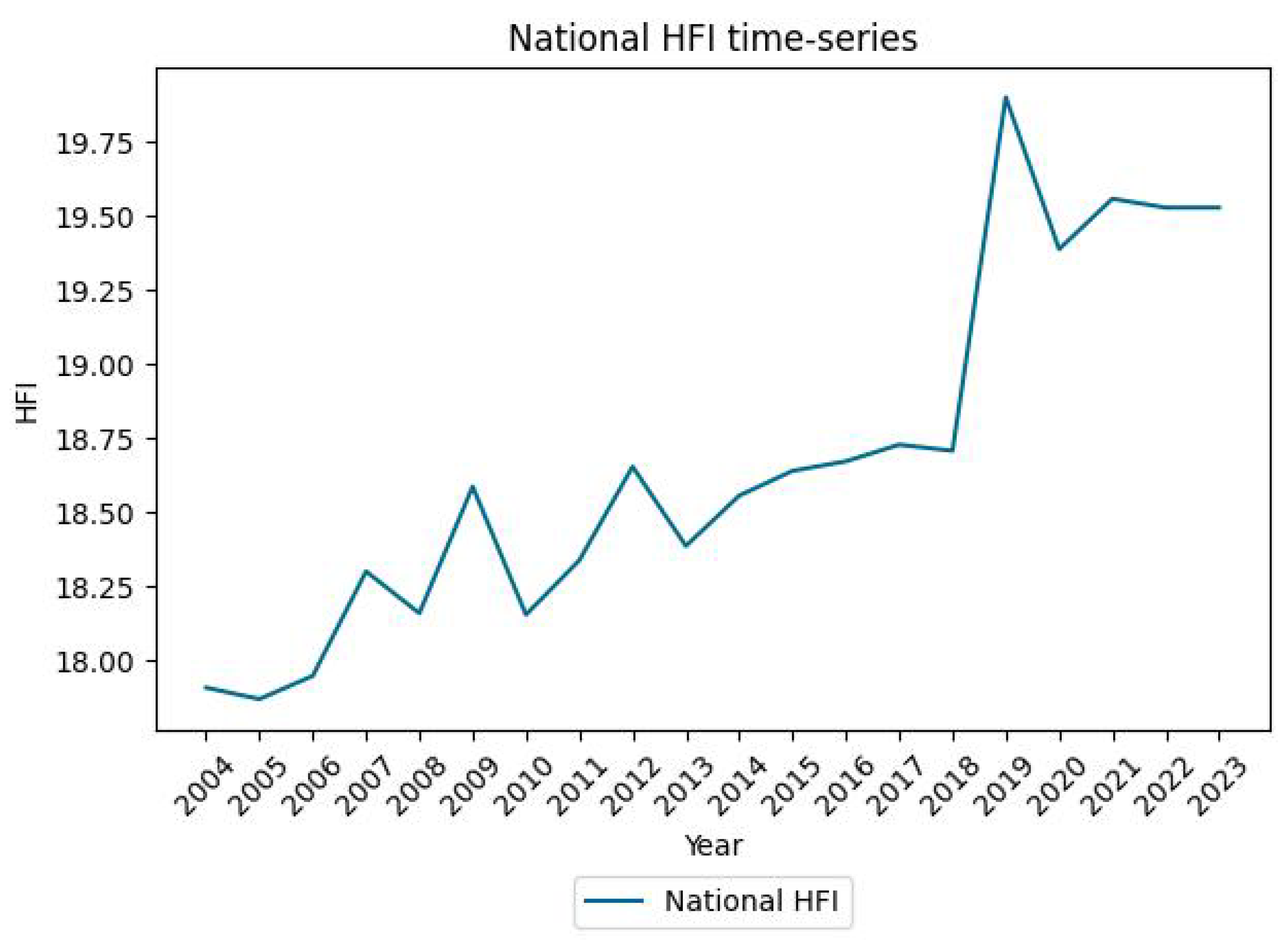
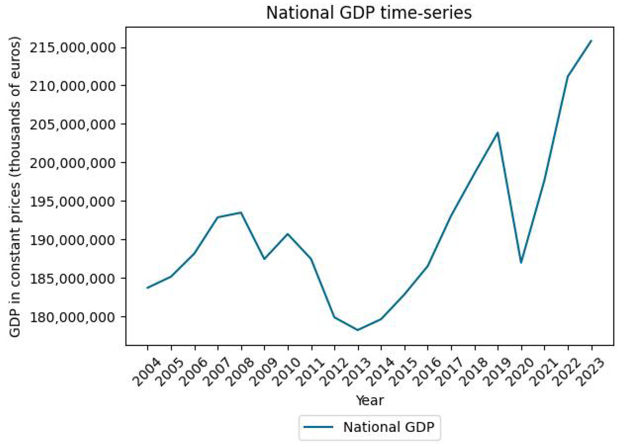
Appendix C. HFI and GDP Time Series at the National Scale
Figure A1.
Evolution of the Portuguese National HFI.
Figure A2.
Evolution of the Portuguese National GDP.
References
- Steffen, W.; Broadgate, W.; Deutsch, L.; Gaffney, O.; Ludwig, C. The trajectory of the Anthropocene: The great acceleration. Anthr. Rev. 2015, 2, 81–98. [Google Scholar] [CrossRef]
- Ellis, E.C.; Ramankutty, N. Putting people in the map: Anthropogenic biomes of the world. Front. Ecol. Environ. 2008, 6, 439–447. [Google Scholar] [CrossRef]
- Almond, R.; Grooten, M.; Juffe Bignoli, D.; Petersen, T. Living Planet Report 2022—Building a Nature Positive Society; Technical Report; WWF: Gland, Switzerland, 2022. [Google Scholar]
- Díaz, S.; Fargione, J.; Chapin, F.S., III; Tilman, D. Biodiversity loss threatens human well-being. PLoS Biol. 2006, 4, e277. [Google Scholar] [CrossRef] [PubMed]
- Díaz, S.; Demissew, S.; Carabias, J.; Joly, C.; Lonsdale, M.; Ash, N.; Larigauderie, A.; Adhikari, J.R.; Arico, S.; Báldi, A.; et al. The IPBES Conceptual Framework—Connecting nature and people. Curr. Opin. Environ. Sustain. 2015, 14, 1–16. [Google Scholar] [CrossRef]
- Haines-Young, R.; Potschin, M. The links between biodiversity, ecosystem services and human well-being. In Ecosystem Ecology: A New Synthesis; Raffaelli, D.G., Frid, C.L.J., Eds.; Ecological Reviews; Cambridge University Press: Cambridge, UK, 2010; pp. 110–139. [Google Scholar]
- Haines-Young, R.; Potschin, M. Common International Classification of Ecosystem Services; Centre for Environmental Management, University of Nottingham: Nottingham, UK, 2012. [Google Scholar]
- Rodríguez, J.P.; Beard, T.D., Jr.; Bennett, E.M.; Cumming, G.S.; Cork, S.J.; Agard, J.; Dobson, A.P.; Peterson, G.D. Trade-offs across space, time, and ecosystem services. Ecol. Soc. 2006, 11, 14. [Google Scholar] [CrossRef]
- Elmqvist, T.; Tuvendal, M.; Krishnaswamy, J.; Hylander, K. Managing trade-offs in ecosystem services. In Values, Payments and Institutions for Ecosystem Management; Edward Elgar Publishing: Cheltenham, UK, 2013; pp. 70–89. [Google Scholar]
- Trauger, D.L.; Czech, B.; Erickson, J.D.; Garrettson, P.R.; Kernohan, B.J.; Miller, C.A. The Relationship of Economic Growth to Wildlife Conservation; Vol. 03-1, The Wildlife Society: Bethesda, MD, USA, 2003. [Google Scholar]
- Sanderson, E.W.; Jaiteh, M.; Levy, M.A.; Redford, K.H.; Wannebo, A.V.; Woolmer, G. The human footprint and the last of the wild. BioScience 2002, 52, 891–904. [Google Scholar] [CrossRef]
- Sanderson, E.W.; Fisher, K.; Robinson, N.; Sampson, D.; Duncan, A.; Royte, L. The March of the Human Footprint. 2022. Available online: https://ecoevorxiv.org/repository/view/3641/ (accessed on 4 August 2024).
- Venter, O.; Sanderson, E.W.; Magrach, A.; Allan, J.R.; Beher, J.; Jones, K.R.; Possingham, H.P.; Laurance, W.F.; Wood, P.; Fekete, B.M.; et al. Global terrestrial Human Footprint maps for 1993 and 2009. Sci. Data 2016, 3, 1–10. [Google Scholar] [CrossRef]
- Dynan, K.; Sheiner, L.; GDP as a Measure of Economic Well-Being. Technical Report, Hutchins Center Working Paper. 2018. Available online: https://www.degruyterbrill.com/document/doi/10.7208/chicago/9780226836348-002/pdf (accessed on 11 October 2024).
- Meadows, D.H.; Meadows, D.L.; Randers, J.; Behrens, W.W. The Limits to Growth: A Report for the Club of Rome’s Project on the Predicament of Mankind; Universe Books: New York, NY, USA, 1972. [Google Scholar]
- Asafu-Adjaye, J. Biodiversity loss and economic growth: A cross-country analysis. Contemp. Econ. Policy 2003, 21, 173–185. [Google Scholar] [CrossRef]
- Gren, I.M.; Campos, M.; Gustafsson, L. Economic development, institutions, and biodiversity loss at the global scale. Reg. Environ. Change 2016, 16, 445–457. [Google Scholar] [CrossRef]
- Martínez-Alier, J.; Pascual, U.; Vivien, F.D.; Zaccai, E. Sustainable de-growth: Mapping the context, criticisms and future prospects of an emergent paradigm. Ecol. Econ. 2010, 69, 1741–1747. [Google Scholar] [CrossRef]
- Schneider, F.; Kallis, G.; Martinez-Alier, J. Crisis or opportunity? Economic degrowth for social equity and ecological sustainability. Introduction to this special issue. J. Clean. Prod. 2010, 18, 511–518. [Google Scholar] [CrossRef]
- UNEP. Decoupling Natural Resource Use and Environmental Impacts from Economic Growth. A Report of the Working Group on Decoupling to the International Resource Panel; UNEP: Nairobi, Kenya, 2011. [Google Scholar]
- Wiedenhofer, D.; Virág, D.; Kalt, G.; Plank, B.; Streeck, J.; Pichler, M.; Mayer, A.; Krausmann, F.; Brockway, P.; Schaffartzik, A.; et al. A systematic review of the evidence on decoupling of GDP, resource use and GHG emissions, part I: Bibliometric and conceptual mapping. Environ. Res. Lett. 2020, 15, 063002. [Google Scholar] [CrossRef]
- Dietz, S.; Adger, W. Economic growth, biodiversity loss and conservation effort. J. Environ. Manag. 2003, 68, 23–35. [Google Scholar] [CrossRef] [PubMed]
- Mitic, P.; Kojic, M.; Minović, J. A Literature Survey of the Environmental Kuznets Curve. Econ. Anal. 2019, 52, 109–127. [Google Scholar] [CrossRef]
- Gregory, R.D.; Van Strien, A.; Vorisek, P.; Gmelig Meyling, A.W.; Noble, D.G.; Foppen, R.P.; Gibbons, D.W. Developing indicators for European birds. Philos. Trans. R. Soc. B Biol. Sci. 2005, 360, 269–288. [Google Scholar] [CrossRef]
- Pereira, H.M.; Cooper, H.D. Towards the global monitoring of biodiversity change. Trends Ecol. Evol. 2006, 21, 123–129. [Google Scholar] [CrossRef]
- Burns, F.; Eaton, M.A.; Burfield, I.J.; Klvaňová, A.; Šilarová, E.; Staneva, A.; Gregory, R.D. Abundance decline in the avifauna of the European Union reveals cross-continental similarities in biodiversity change. Ecol. Evol. 2021, 11, 16647–16660. [Google Scholar] [CrossRef]
- Jenks, G.F. The data model concept in statistical mapping. Int. Yearb. Cartogr. 1967, 7, 186–190. [Google Scholar]
- Alonso, H.; Coelho, R.; Gouveia, C.; Rethoré, G.; Teodósio, J. Relatório do Censo de Aves Comuns 2004–2023; Technical Report; Sociedade Portuguesa para o Estudo das Aves: Lisboa, Portugal, 2024. [Google Scholar]
- Mu, H.; Li, X.; Wen, Y.; Huang, J.; Du, P.; Su, W.; Miao, S.; Geng, M. A global record of annual terrestrial Human Footprint dataset from 2000 to 2018. Sci. Data 2022, 9, 176. [Google Scholar] [CrossRef]
- AMECO Database. Available online: https://economy-finance.ec.europa.eu/economic-research-and-databases/economic-databases/ameco-database_en (accessed on 27 June 2024).
- Statistics Portugal. Available online: https://www.ine.pt/xportal/xmain?xpid=INE&xpgid=ine_cnacionais2010b2016&menuBOUI=13707095&contexto=cr&selTab=tab3&perfil=392023561&INST=391966542 (accessed on 28 August 2024).
- Pannekoek, J.; Van Strien, A. TRIM 3 Manual (TRends & Indices for Monitoring Data); Statistics Netherlands: Voorburg, The Netherlands, 2005. [Google Scholar]
- Soldaat, L.L.; Pannekoek, J.; Verweij, R.J.; van Turnhout, C.A.; van Strien, A.J. A Monte Carlo method to account for sampling error in multi-species indicators. Ecol. Indic. 2017, 81, 340–347. [Google Scholar] [CrossRef]
- Pannekoek, J.; Bogaart, P.; van der Loo, M. Models and Statistical Methods in Rtrim; Statistics Netherlands: The Hague, The Netherlands, 2018. [Google Scholar]
- Pesaran, H.; Shin, Y. An Autoregressive Distributed Lag Modeling Approach to Co-integration Analysis. In Econometncs and Economic Theory in the 20st Century: The Ragnar Frisch Centennial Symposium; Department of Applied Economics, University of Cambridge: Cambridge, UK, 1995; Volume 31. [Google Scholar]
- Pesaran, M.H.; Shin, Y.; Smith, R.J. Bounds testing approaches to the analysis of level relationships. J. Appl. Econom. 2001, 16, 289–326. [Google Scholar] [CrossRef]
- Akaike, H. A new look at the statistical model identification. IEEE Trans. Autom. Control. 1974, 19, 716–723. [Google Scholar] [CrossRef]
- Scholes, R.J.; Reyers, B.; Biggs, R.; Spierenburg, M.; Duriappah, A. Multi-scale and cross-scale assessments of social–ecological systems and their ecosystem services. Curr. Opin. Environ. Sustain. 2013, 5, 16–25. [Google Scholar] [CrossRef]
- Mori, A.S.; Isbell, F.; Cadotte, M.W. Assessing the importance of species and their assemblages for the biodiversity-ecosystem multifunctionality relationship. Ecology 2023, 104, e4104. [Google Scholar] [CrossRef]
- Rigal, S.; Dakos, V.; Alonso, H.; Auniņš, A.; Benko, Z.; Brotons, L.; Chodkiewicz, T.; Chylarecki, P.; De Carli, E.; Del Moral, J.C.; et al. Farmland practices are driving bird population decline across Europe. Proc. Natl. Acad. Sci. USA 2023, 120, e2216573120. [Google Scholar] [CrossRef]
- Gregory, R.D.; Skorpilova, J.; Vorisek, P.; Butler, S. An analysis of trends, uncertainty and species selection shows contrasting trends of widespread forest and farmland birds in Europe. Ecol. Indic. 2019, 103, 676–687. [Google Scholar] [CrossRef]
- Gregory, R.D.; Eaton, M.A.; Burfield, I.J.; Grice, P.V.; Howard, C.; Klvaňová, A.; Noble, D.; Šilarová, E.; Staneva, A.; Stephens, P.A.; et al. Drivers of the changing abundance of European birds at two spatial scales. Philos. Trans. R. Soc. B 2023, 378, 20220198. [Google Scholar] [CrossRef]
- Reif, J. Long-term trends in bird populations: A review of patterns and potential drivers in North America and Europe. Acta Ornithol. 2013, 48, 1–16. [Google Scholar] [CrossRef]
- Reif, J.; Gamero, A.; Hološková, A.; Aunins, A.; Chodkiewicz, T.; Hristov, I.; Kurlavičius, P.; Leivits, M.; Szép, T.; Voříšek, P. Accelerated farmland bird population declines in European countries after their recent EU accession. Sci. Total Environ. 2024, 946, 174281. [Google Scholar] [CrossRef]
- Kerr, J.T.; Currie, D.J. Effects of human activity on global extinction risk. Conserv. Biol. 1995, 9, 1528–1538. [Google Scholar] [CrossRef]
- Mozumder, P.; Berrens, R.P.; Bohara, A.K. Is there an environmental Kuznets curve for the risk of biodiversity loss? J. Dev. Areas 2006, 39, 175–190. [Google Scholar]
- Mikkelson, G.M.; Gonzalez, A.; Peterson, G.D. Economic inequality predicts biodiversity loss. PLoS ONE 2007, 2, e444. [Google Scholar] [CrossRef]
Disclaimer/Publisher’s Note: The statements, opinions and data contained in all publications are solely those of the individual author(s) and contributor(s) and not of MDPI and/or the editor(s). MDPI and/or the editor(s) disclaim responsibility for any injury to people or property resulting from any ideas, methods, instructions or products referred to in the content. |
© 2025 by the authors. Licensee MDPI, Basel, Switzerland. This article is an open access article distributed under the terms and conditions of the Creative Commons Attribution (CC BY) license (https://creativecommons.org/licenses/by/4.0/).