A Fault Diagnosis Method for Pump Station Units Based on CWT-MHA-CNN Model for Sustainable Operation of Inter-Basin Water Transfer Projects

Abstract

Inter-basin water transfer projects are core infrastructure for achieving sustainable water resource allocation and addressing regional water scarcity, and pumping station units, as their critical energy-consuming and operation-controlling components, are vital to the projects’ sustainable performance. With the growing complexity and scale of these projects, pumping station units have become more intricate, leading to a gradual rise in failure rates. However, existing fault diagnosis methods are relatively backward, failing to promptly detect potential faults—this not only threatens operational safety but also undermines sustainable development goals: equipment failures cause excessive energy consumption (violating energy efficiency requirements for sustainability), unplanned downtime disrupts stable water supply (impairing reliable water resource access), and even leads to water waste or environmental risks. To address this sustainability-oriented challenge, this paper focuses on the fault characteristics of pumping station units and proposes a comprehensive and accurate fault diagnosis model, aiming to enhance the sustainability of water transfer projects through technical optimization. The model utilizes advanced algorithms and data processing technologies to accurately identify fault types, thereby laying a technical foundation for the low-energy, reliable, and sustainable operation of pumping stations. Firstly, continuous wavelet transform (CWT) converts one-dimensional time-domain signals into two-dimensional time-frequency graphs, visually displaying dynamic signal characteristics to capture early fault features that may cause energy waste. Next, the multi-head attention mechanism (MHA) segments the time-frequency graphs and correlates feature-location information via independent self-attention layers, accurately capturing the temporal correlation of fault evolution—this enables early fault warning to avoid prolonged inefficient operation and energy loss. Finally, the improved convolutional neural network (CNN) layer integrates feature information and temporal correlation, outputting predefined fault probabilities for accurate fault determination. Experimental results show the model effectively solves the difficulty of feature extraction in pumping station fault diagnosis, considers fault evolution timeliness, and significantly improves prediction accuracy and anti-noise performance. Comparative experiments with three existing methods verify its superiority. Critically, this model strengthens sustainability in three key ways: (1) early fault detection reduces unplanned downtime, ensuring stable water supply (a core sustainable water resource goal); (2) accurate fault localization cuts unnecessary maintenance energy consumption, aligning with energy-saving requirements; (3) reduced equipment failure risks minimize water waste and environmental impacts. Thus, it not only provides a new method for pumping station fault diagnosis but also offers technical support for the sustainable operation of water conservancy infrastructure, contributing to global sustainable development goals (SDGs) related to water and energy.

1. Introduction

The pumping unit is the core equipment of the pumping station, and its operating condition directly affects the safety of the pumping station. The failure mechanism of the pumping station unit is complex, there are many types of failures, and the failures are often coupled with each other, with a variety of unique failure characteristics [1,2,3]. As the size and complexity of pumping station units continue to increase, the dimensionality of pumping station operational data gradually increases, and the correlation between attributes becomes more complex [4]. Traditional shallow learning methods are inefficient in extracting features from acquired signals and cannot effectively cope with high-dimensional data problems [5,6]. Furthermore, the evolution of faults exhibits significant temporal characteristics, with the current fault often being the result of changes in the system’s state at the previous moment [7,8]. Therefore, capturing temporal information in the data is crucial for improving the accuracy of fault diagnosis. In recent years, bearing fault diagnosis methods based on machine learning (ML) have been widely applied, but this method still requires operators to possess professional knowledge and signal processing techniques, and the existing feature extraction methods do not have universality [9]. Furthermore, traditional machine learning algorithms exhibit obvious limitations when dealing with the non-linear relationships between features [10,11]. Therefore, in view of the complexity of signal feature extraction for pumping station units and the uncertainty of fault evolution, the development of an efficient fault diagnosis method has important practical significance.

Deep Learning (DL) theory was proposed by Hinton et al. in 2006 [12]. Through a deep architecture of multi-layer data processing units, it can learn multi-level representations from input data [13]. Thanks to its powerful feature extraction and learning capabilities, this technology has developed rapidly and achieved significant breakthroughs in the fields of speech recognition and computer vision [14,15]. Convolutional Neural Networks (CNN), as an important technique of deep learning, was first applied in the field of image recognition [16]. Krizhevsky et al. combined convolutional neural networks with deep learning theory, proposing the “AlexNet” network structure [17]. CNNs extract features layer by layer, abstracting features from shallow to deep, and can automatically perform feature extraction, and its unique network structure can effectively retain data features [18]. Therefore, CNNs have attracted widespread attention from scholars in the field of fault diagnosis. Levent et al. [19] adopted an adaptive 1D-CNN classifier, taking data with time attributes as input, and designed a real-time bearing fault diagnosis system. Miyazaki et al. [20] proposed a fault diagnosis method combining an improved statistical filter (SF) and CNN, which can effectively extract fault signals from strong background noise and input them into the CNN for analysis. Wang et al. [21] constructed a multi-scale learning neural network, learning local correlations in adjacent and non-adjacent intervals in bearing vibration signals through convolutional channels.

Despite the promising results achieved by CNNs in the field of fault diagnosis, there are still some issues. Firstly, the input format of the CNN can have a certain impact on its performance [22,23,24]; it is better at processing image data, capable of effectively preserving image features and performing dimensionality reduction [25]. As the number of layers increases, the performance of deep models may decrease due to the problem of vanishing or exploding gradients [26,27]. CNNs are not particularly good at processing time-series data. Time-series data usually has temporal dependencies and continuity, therefore the model must be able to capture the associations between different time points in the sequence [28].

To resolve the aforementioned challenges, we present a hybrid model integrating Continuous Wavelet Transform (CWT), Multi-Head-Attention (MHA), and an enhanced CNN. The model employs CWT to convert signals into time-frequency representations, while MHA processes these representations in segmented blocks to mitigate information loss in lengthy sequential data during training. This approach also captures long-range dependencies across the input feature maps, strengthening temporal relationships. The CNN layer then synthesises the extracted features and temporal correlations to predict the likelihood of each predefined fault. To validate the model’s superiority and its noise resilience for real-world deployment, comparisons are drawn against established fault diagnosis methods (e.g., CNN, GRU, LSTM) using both pristine and synthetically noised datasets. This paper selects CNN, LSTM and GRU as the benchmark models because they represent the three core paradigms of fault diagnosis—CNN is used for local feature extraction (matching our time-frequency graph input), and LSTM/GRU is used for sequential dependence (adapting to the temporality of vibration signals)—their effectiveness has been fully verified in the fault diagnosis of rotating machinery. Ensured relative effectiveness. For targeted reasons, we excluded other state-of-the-art models: the Visual Transformer (ViT) requires a large number of labeled samples (which is impractical for pump failure scenarios with limited data) and may overlook local subtle fault features; ResNet (a variant of deep CNN) increases the computational complexity but does not offer significant gains because our improved CNN with SE concerns has already met the feature extraction requirements of pumping station signals. Graph neural networks (GNNS) rely on topological data relationships, which are redundant here—our three-axis sensor data unifies the time-frequency graph through CWT, making topological modeling of GNNS unnecessary. Therefore, the selected baseline covers core technology paradigms and excludes other models to balance experimental validity, engineering applicability and efficiency. Experimental outcomes demonstrate marked performance gains in diagnosing faults within complex systems, affirming the model’s efficacy.

The principal contributions of this work are summarised below:

(1)

CWT transmutes vibrational features and temporal data from pump station bearings into 2D image formats, aligning with CNN processing strengths and furnishing robust diagnostic inputs.

(2)

MHA bolsters temporal coherence, counteracting CNN shortcomings in sequential data handling, curbing parameter bloat and data loss, and adeptly tracking system dynamics to address fault progression timelines.

(3)

CNN refinements include batch normalisation post-convolution for training stability and dropout post-full-connection to avert overfitting. Crucially, the SE attention mechanism after the second convolutional layer prioritises salient features via channel-wise weighting, elevating diagnostic precision.

Consequently, our MHA-CNN fusion model for complex system fault diagnosis adeptly unifies feature extraction with temporal fault evolution tracking.

2. A Fault Diagnosis Model for Pump Station Units Based on Deep Learning

2.1. Continuous Wavelet Transform (CWT)

CWT is a time-frequency localisation tool that calculates the spectrum of the signal within each window by sliding a window of adjustable length along the time axis, thereby obtaining a time-frequency representation of the original signal. Due to the presence of a scaling factor, CWT can adjust the window length to adapt to the local characteristics of different frequency components, making it suitable for analysing non-stationary signals [29,30,31,32]. In this paper, 2D-CWT is employed to process the vibration signals of pumping station units. For the square-integrable signal $x(t)$ it can be expressed as:

$$W_x(a,b)={\displaystyle \int x(t){\psi }_{a,b}(t)dt=\frac{1}{\sqrt{a}}}{\displaystyle \int x(t){\psi }^{\prime }(\frac{t-b}{a})dt}$$

(1)

where $a$ represents the scaling factor, b represents the time location, ${\psi }_{a,b}(t)$ is the mother wavelet function, and ${{\psi }^{\prime }}_{a,b}(t)$ is the complex conjugate of the mother wavelet. The expression of the mother wavelet is as follows:

$${\psi }_{a,b}(t)={\displaystyle \frac{1}{\sqrt{a}}}\psi ({\displaystyle \frac{t-b}{a}})$$

(2)

In CWT, the time and frequency resolution change with the scaling factor. In the low-frequency part of the signal, the frequency resolution is higher, and the time resolution is lower; while in the high-frequency part, the opposite is true. This is consistent with the characteristics of low-frequency signals changing slowly and high-frequency signals changing quickly.

2.2. Improved Convolutional Neural Network (CNN)

2.2.1. SE Attention Mechanism Module

Proposed by Hu [33], the SE (Squeeze-and-Excitation) layer constitutes a lightweight attention module that intensifies focus on diagnostically relevant time-frequency feature map channels while attenuating less pertinent ones along the channel dimension, thereby enhancing classification accuracy. As illustrated in Figure 1, this attention mechanism operates through three principal stages: Squeeze, Excitation and Reweight.

Squeeze operation: The data dimensions of the input channel are compressed, reducing the multidimensional data to a single value. The calculation formula is as follows:

$${\mathrm{z}}_{\mathrm{c}}={\displaystyle \frac{1}{L}}{\displaystyle \sum _{\mathrm{j}}^L{\mathrm{x}}_{\mathrm{c}}\left(j\right)}$$

(3)

where: ${\mathrm{z}}_{\mathrm{c}}$ is the output after compression; $L$ is the product of height H and width W; ${\mathrm{x}}_{\mathrm{c}}$ is the eigenvalue on the feature graph in channel $\mathrm{c}$.

Excitation operation: Each feature channel generates the corresponding feature weight. The calculation formula is shown below:

$${\mathrm{s}}_{\mathrm{c}}=\delta \{{\sigma }_{\mathrm{j}+1}\left[\mathrm{Re}LU({\sigma }_{\mathrm{j}+1}{\mathrm{z}}_{\mathrm{c}})\right]$$

(4)

where: ${\sigma }_{\mathrm{j}}$, ${\mathrm{z}}_{\mathrm{c}}$ is the output of the jth-layer fully connected layer, which is processed by ReLU activation function, and then processed by j + 1 layer fully connected layer, and finally the weights is obtained by Sigmoid function $\delta$.

Reweight operation: The weights generated by the Excitation operation are weighted to the input feature layer one by channel. The formula is as follows:

$$\mathrm{p}={\mathrm{x}}_{\mathrm{c}}{\mathrm{s}}_{\mathrm{c}}$$

(5)

2.2.2. Improve the Structure and Parameters of CNN

Convolutional Neural Networks (CNNs) employ convolution operations to extract features, offering both computational efficiency and robustness against interference. The architecture consists of five principal components: the data input layer, convolutional feature extraction layer, dimensionality reduction layer, fully connected classification layer, and output layer [34]. This study utilises a CNN derived from the classic LeNet-5 framework, enhanced with batch normalisation (BN) following convolutional layers and dropout after fully connected layers to mitigate overfitting, supplemented by an SE attention module after the second convolutional layer. As illustrated in Figure 2, the refined CNN architecture comprises an input layer, two convolutional layers (C1, C2), two pooling layers (P1, P2), an SE attention layer (S1), and three fully connected layers (F1, F2, F3). Informed by findings from reference [35] and LeNet-5′s parameter optimisation methodology, The parameter Settings of the CNN layer in this study are based on three criteria: First, referring to the classic framework of LeNet-5 in image feature extraction, combined with the feature density of the pump station vibration time-frequency graph (at a resolution of 256 × 256, the 5 × 5 convolution kernel can effectively capture local fault details such as the spatio-temporal distribution of impact pulses, and the 2 × 2 pooling can retain key time-frequency information while reducing dimension and avoid feature dilution); The second is the optimization rule of CNN parameters for fault signals of rotating machinery. Six initial convolution kernels can cover the harmonic features of low-order faults, and 16 deep convolution kernels can further extract the features of high-order coupled faults (such as the composite frequency components of misalignment—friction coupling faults). Thirdly, through comparative experiments (testing 3 × 3/7 × 7 convolution kernels and 1 × 1/3 × 3 pooling kernels), the current parameters perform the best in terms of model convergence speed and fault classification accuracy. Moreover, after the SE attention layer is set at the C2 layer, channel weighting can be carried out for complex features extracted from deep layers to enhance the focus on fault-sensitive channels,

Table 1. Network parameter.

Network Layer	Description	Output Feature Map Size
Input layer	Input data	256 × 256 × 3
Convolution layer (C1) + BN layer	6 Filter 5 × 5	256 × 256 × 6
Pooling layer (P1)	Filter 2 × 2	128 × 128 × 6
Convolution layer (C2) + BN layer	16 Filter, 5 × 5	128 × 128 × 16
Pooling layer (P2)	Filter 2 × 2	64 × 64 × 16
SE layer (S1)	_	64 × 64 × 16
Fully connected layer (F1)	128 nodes, Dropout = 0.5	128 × 65,536
Fully connected layer (F2)	64 nodes, Dropout = 0.5	64 × 128
Fully connected layer (F3)	12 nodes	12 × 64
Output layer	_	12 × 1
Learning rate	0.0001

presents the definitive network configuration. The system processes 256 × 256 × 3 dimensional time-frequency images as input, yielding 7 × 1 dimensional outputs. The C1 layer’s 6 convolutional kernels produce 256 × 256 × 6 feature maps, downsampled to 128 × 128 × 6 by P1. C2′s 16 kernels generate 128 × 128 × 16 features, subsequently reduced to 64 × 64 × 16 through P2 pooling.

2.3. Multi Head Attention Mechanism (MHA)

2.3.1. MHA Structure

While CNNs excel at processing local features, their ability to model long-range dependencies remains constrained. MHA addresses this limitation by computing correlations across all positions—regardless of spatial separation—thereby facilitating global feature interactions. This mechanism allows MHA to extract long-term dependencies from any region of the input feature map, proving particularly effective for signals with intricate patterns by capturing cross-regional relationships and integrating broader contextual information. Consequently, it enhances convolutional networks’ capacity to interpret complex patterns, leading to improved model performance [36].

The number of heads (i.e., the number of “heads” in multi-head attention) is an important hyperparameter, and its setting will affect the performance, computational efficiency and expressive power of the model. The embedding dimension ($d_{model}$) of the quantitative model of the head is usually interrelated. Under normal circumstances, the number of heads should make the dimension ($d_k$) of each head reasonable, that is, the embedding dimension must be divisible by the number of avatars to ensure uniform feature segmentation among avatars. The formula is:

$$d_k={\displaystyle \frac{d_{model}}{h}}$$

(6)

In the formula, the embedding dimension of the model is $d_{model}$, the number of heads is $h$, and the dimension of the heads is $d_k$.

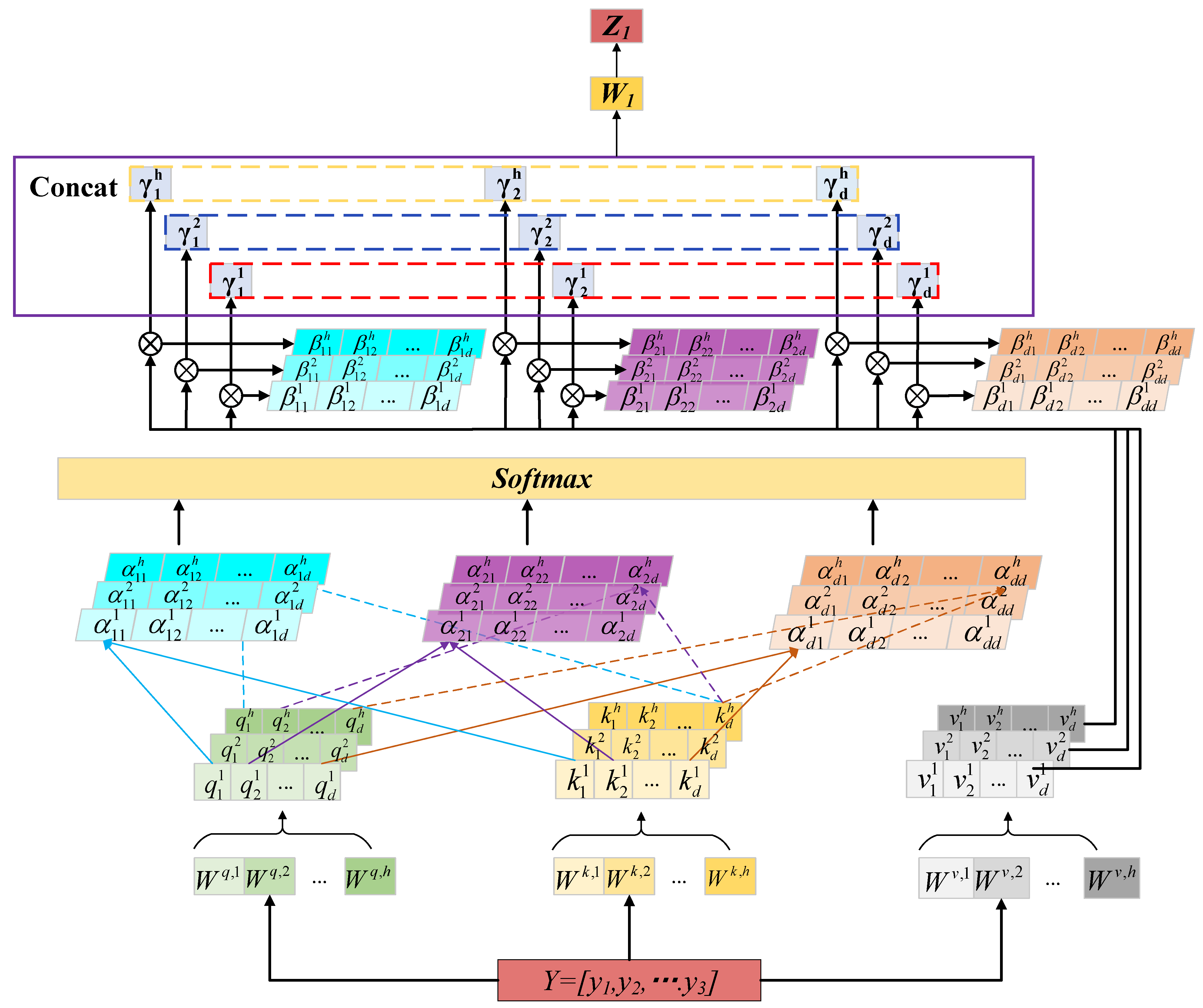
Based on the input data features of this paper (the 256 × 256 × 3 time-frequency graph converted by CWT, and the corresponding feature embedding dimensions need to match the dimension splitting logic of multi-head attention), according to the principle in Formula (6), the three attention heads can evenly split the feature dimensions of each head (avoiding feature fragmentation caused by information overload of a single head or too small multi-head dimensions). Meanwhile, through the control variable experiment verification (testing the model performance of the 1, 2, and 4 attention heads), the 3 attention heads achieved the optimal balance between capturing the long-range dependence of the pump station vibration signal (such as the temporal correlation of fault evolution) and controlling the number of model parameters (to avoid the decline in training efficiency caused by excessive complexity). It can, respectively, focus on the mid-frequency band (Head1), high-frequency band (Head2) and low-frequency band (Head3) characteristics of the time-frequency graph, covering the main frequency components of the pump station fault signal (such as the mid-low frequency characteristics of rotor misconnection and the high-frequency impact characteristics of dynamic and static friction). Therefore, three headers were set based on the experimental data dimensions of this article. As shown in Figure 3, the MHA mechanism uses multiple independent self-attention layers to correlate all the features and temporal location information of the input sequence, and outputs more associated information through weighting.

Assuming a set of input sequences $Y=[y_1,y_2\dots y_d]$, according to Figure 3, we can first derive the query vector $Q^i$, key vector $K^i$, value vector $V^i$, and the linear transformations matrices $W^{q,i}$, $W^{k,i}$, $W^{v,i}$ for query, key and value of the i-th head.

$$Q^i=Y{W}^{q,i}=\left[q_1^i,q_2^i,\dots ,q_d^i\right]$$

(7)

$$K^i=Y{W}^{k,i}=\left[k_1^i,k_2^i,\dots ,k_d^i\right]$$

(8)

$$V^i=Y{W}^{v,i}=\left[v_1^i,v_2^i,\dots ,v_d^i\right]$$

(9)

Value vector $K^i$ to obtain the corresponding weight ${\alpha }_{mn}^i$ and then normalize it using the Softmax function to obtain ${\beta }_{mn}^i$.

$${\alpha }_{mn}^i={\displaystyle \frac{q_m^i\cdot k_n^i}{\sqrt{d_k}}}$$

(10)

$${\beta }_{mn}^i=\mathrm{Softmax}({\alpha }_{mn}^i)$$

(11)

where ${\displaystyle \frac{1}{\sqrt{d_k}}}$ is the scaling factor used in the Softmax function computation to keep the gradient from dissolving. The coefficient of attention is:

$${\gamma }_m^i={\displaystyle \sum _{n=1}^d{\beta }_{mn}^i\cdot v_n^i}$$

(12)

$$hea{d}_i=Attention(Q^i,K^i,V^i)=\left[{\gamma }_1^i,{\gamma }_2^i,\dots ,{\gamma }_d^i\right]$$

(13)

$$Z_t=MultiHead(Q,K,V)=Concat(hea{d}_1,hea{d}_2,\dots ,hea{d}_h)W^h$$

(14)

The overall output is obtained by the Switch activation function through a fully connected output layer. The formula is as follows:

$$Outputs=Swish(Z_i)={\displaystyle \frac{Z_i}{1+e^{-Z_i}}}$$

(15)

2.3.2. MHA Processes Data

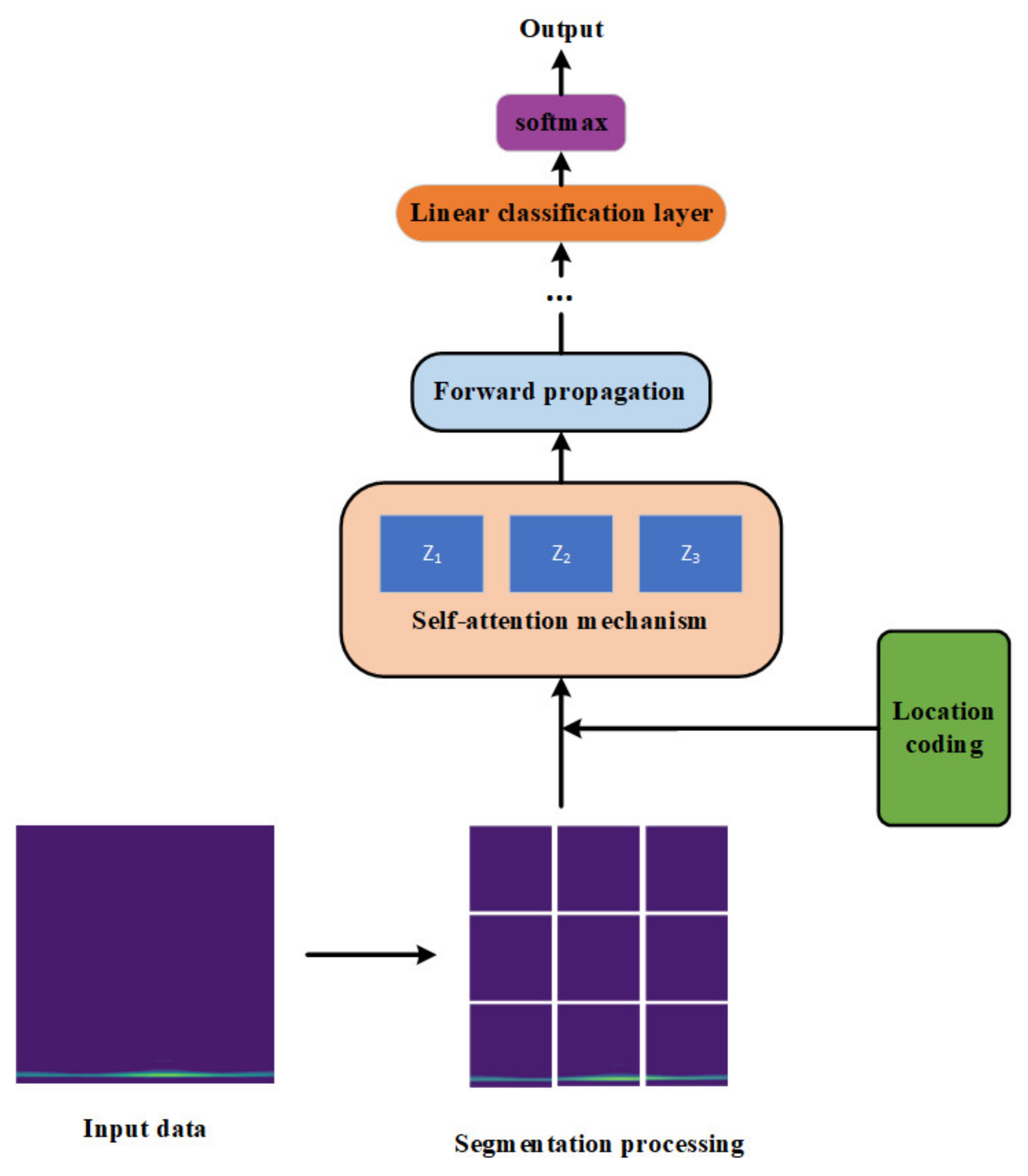
For fault diagnosis applications, sensor-collected one-dimensional time-domain signals serve as the input data. However, lengthy time-domain datasets pose challenges: they not only introduce excessive parameters during model training but may also compromise contextual information at the data boundaries. Drawing inspiration from the Multi-Head Attention (MHA) mechanism’s implementation in computer vision—particularly its use in Vision Transformer (ViT) models for image patching—this study explores analogous segmentation approaches for vibration signal time-frequency representations. The proposed segmentation methodology is visually demonstrated in Figure 4.

The Multi-Head Attention (MHA) mechanism comprises several multi-head attention layers, each consisting of a self-attention layer followed by a fully connected layer. As illustrated in Figure 4, Z1, Z2 and Zn denote the computational outputs from each individual self-attention mechanism. These are computed in parallel and subsequently concatenated to form the self-attention layer’s output. This output then feeds into the fully connected layer, where the extracted feature information undergoes fusion and additional transformation, thereby completing one full multi-head attention layer.

2.4. CWT-MHA-CNN Fault Diagnosis Flow

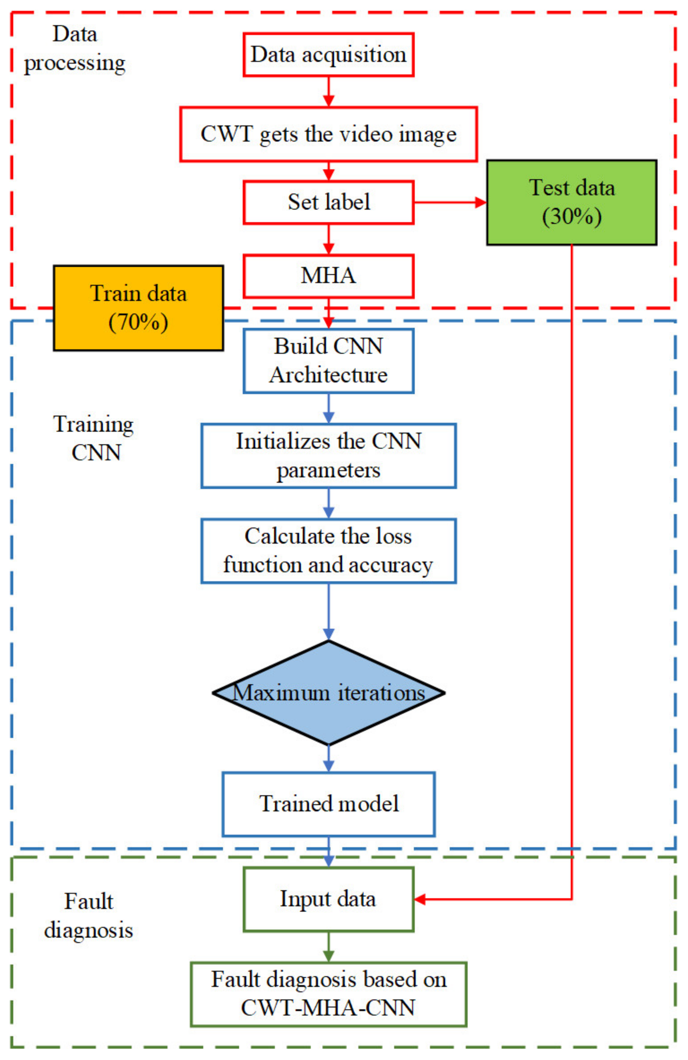
As demonstrated by the preceding analysis, Figure 5 illustrates the CWT-MHA-CNN based fault diagnosis procedure for pumping station units. The process commences with the collection of sensor data from the units, followed by Continuous Wavelet Transform (CWT) time-frequency analysis to produce time-frequency representations. The Multi-Head Attention (MHA) mechanism subsequently partitions these diagrams to mitigate information loss caused by extensive data volumes and parameter complexity, whilst simultaneously strengthening global feature interactions and identifying long-range dependencies through comprehensive positional correlation calculations. The dataset is then partitioned into training and testing subsets (comprising 70% and 30% of the total data, respectively), with the training data serving as input to the enhanced Convolutional Neural Network (CNN). The network’s output provides diagnostic information regarding sensor health status, enabling the identification of potential fault signals.

3. Data Processing

3.1. Collection of Fault Data for Pump Station Units

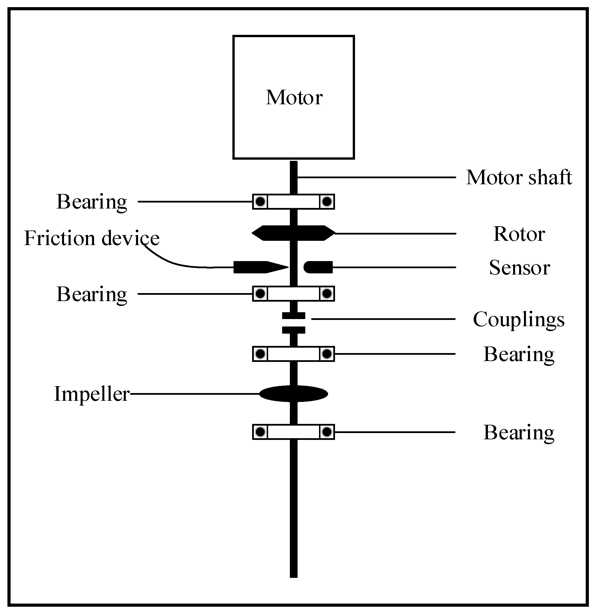
To simulate various real situations of faults in pumping station units, this experiment sets up three fault types: rotor misalignment, rotor-stator friction, and coupling of misalignment and friction, with a sampling frequency of 1000 hz. The sampling length was 7200. A total of 12 fault conditions were constructed based on different rotational speeds. The experiment was carried out on the pump station unit test bench, and the schematic diagram is shown in Figure 6. To accurately capture the vibration characteristics under various working conditions, the experiment adopted a three-axis vibration acceleration sensor for signal acquisition. The sensor was deployed along the horizontal (X-axis), vertical (Y-axis), and axial (Z-axis) directions on the drive end bearing housing and the non-drive end bearing housing of the test bench, respectively—these two locations are the core transmission nodes for the fault vibration of the rotor system. The sensor is rigidly fixed by a magnetic base to ensure synchronous transmission with equipment vibration, and the collected raw signal provides basic data for subsequent fault characteristic analysis. After the signal acquisition deployment is completed, the target fault is simulated in a specific way: a thin ring-shaped gasket with a thickness of 1.0 mm is added at the bearing to generate a preset misalignment between the lower rotor and the upper rotor to simulate the parallel misalignment fault; A brass screw is installed on the test bench above the guide bearing at a distance of 0.2 mm from the rotor. When the rotor rotates at high speed, if the vibration amplitude exceeds the distance between the screw and the rotor, the two will rub against each other, which simulates a rubbing fault.

3.2. Construction of Fault Samples

For the collected signals, 1024 sampling points were selected. Therefore, sub-fragments with a dimension of 1024 were used for sliding slicing to construct the fault sample set. The specific process is shown in Figure 7. After the original collected signals for each working condition are slid and sliced, 36,000 samples are ultimately generated, each of which is a vibration time series signal containing 1024 sampling points. The fault samples of the 12 working conditions constructed are shown in

Table 2. Dataset description.

Fault Type	Speed	Number of Samples	Fault Severity	Category
rotor parallel misalignment (C)	1000	36,000	0.07	0
rotor parallel misalignment (C)	1500	36,000	0.14	1
rotor parallel misalignment (C)	2000	36,000	0.21	2
rotor-stator friction (PM)	1000	36,000	0.07	3
rotor-stator friction (PM)	2000	36,000	0.14	4
rotor-stator friction (PM)	2500	36,000	0.21	5
rotor-stator friction (PM)	3000	36,000	0.28	6
misalignment and friction coupling fault (PMC)	1000	36,000	0.07	7
misalignment and friction coupling fault (PMC)	1500	36,000	0.14	8
misalignment and friction coupling fault (PMC)	2000	36,000	0.21	9
misalignment and friction coupling fault (PMC)	2500	36,000	0.28	10
misalignment and friction coupling fault (PMC)	3000	36,000	0.35	11

. The fault types mainly include rotor parallel misalignment (C), rotor-stator friction (PM), and misalignment and friction coupling fault (PMC). The rotational speed is selected at five key nodes within the range of 1000 to 3000 r/min: 1000, 1500, 2000, 2500, and 3000 r/min. Through the differentiated combination of “fault type + rotational speed”, 12 working conditions (3 types of C type, 4 types of PM type, and 5 types of PMC type) are formed, and each working condition corresponds to a type of “fault-rotational speed” characteristic mode that needs to be precisely identified. The experiment did not present the results of all rotational speeds and was based on the design principle of representative rotational speed coverage: The vibration characteristics of the unit change continuously within 1000–3000 r/min. Selecting the above five key rotational speeds can already cover the differences in fault characteristics in the low, medium and high rotational speed ranges. Moreover, the experiment verifies that this setting can fully reflect the fault evolution law under different loads. Testing other rotational speeds separately will lead to data redundancy and reduce the experimental efficiency. For Type C faults, only three speeds of 1000, 1500, and 2000 r/min are set. This is mainly because the characteristics of this fault are clearer at low and medium speeds, and it is less affected by the electromagnetic noise of the motor and the hydraulic disturbance of the impeller. When the speed exceeds 2000 r/min, the fault characteristics are easily disturbed, making it difficult to extract pure fault signals.

In order to reduce the randomness of classification results, 3000 samples were randomly selected for training for each type of fault, and the remaining 900 samples were tested.

Due to various factors such as hydraulic, mechanical, and electromagnetic factors that may bring noise to fault signals during the actual operation of pump station units, in order to simulate signals collected from real scenarios and evaluate the diagnostic accuracy of fault diagnosis methods based on the CWT-MHA-CNN model for noisy signals, different signal-to-noise ratios of noise were added to the original experimental data, and a fault sample set with different noise levels was constructed. In order to construct a noisy fault sample set, the power of each original experimental fault signal is first calculated, and then Gaussian white noise with a specific signal-to-noise ratio is added. The definition of signal-to-noise ratio is as follows:

$$SN{R}_{\mathrm{d}B}=10{\log }_{10}({\displaystyle \frac{P_s}{P_n}})$$

(16)

Among them, P_s and P_n represent signal power and noise power, respectively.

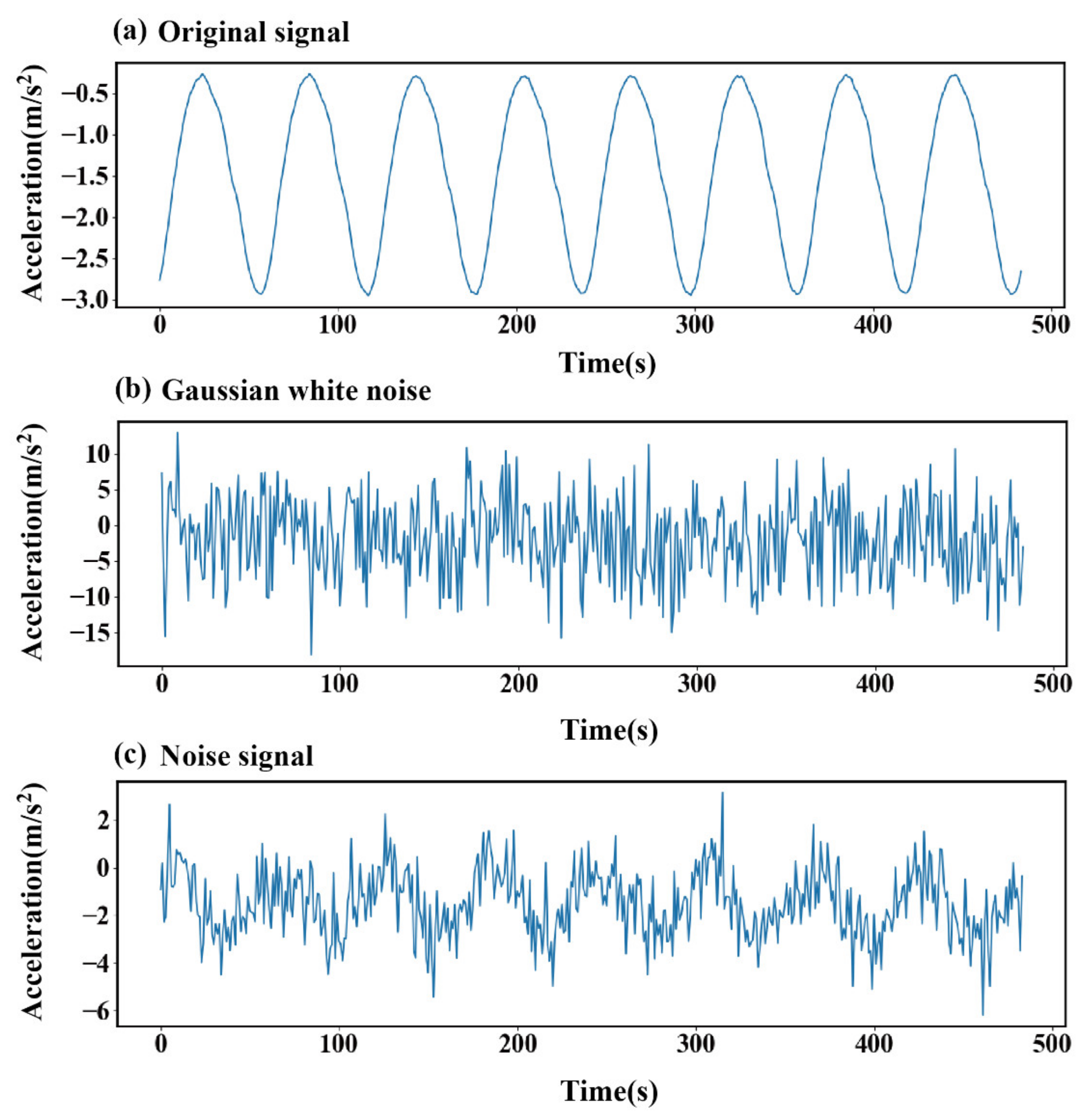
Figure 8 shows a set of original experimental fault signals, Gaussian white noise signals, and fault signal graphs containing Gaussian white noise: Figure 8a shows the original signal, which is derived from the vibration signal collected by the three-axis vibration acceleration sensor at the drive end bearing housing of the pump station unit test bench under normal no-load operation conditions without preset faults. The core components are the fundamental frequency harmonics of the motor and the low-order harmonics of the bearing. The harmonic characteristics of slight interference formed after superimposing the slight vibration of the test bench base and the background noise of the circuit, and this signal has a non-zero average value phenomenon. It is mainly caused by the mechanical static offset caused by the preload force of the test bench bearing and the shafting assembly, as well as the low-frequency zero drift of the sensor and the DC component introduced by the offset of the front-end circuit of the acquisition card. However, this non-zero average value belongs to the static baseline offset. It is independent of the dynamic fault characteristics. The subsequent CWT time-frequency conversion can be effectively separated without interfering with the model performance. Figure 8b shows the Gaussian white noise signal, which is the noise source for the subsequent construction of the noisy sample. Figure 8c shows the fault signal containing Gaussian white noise, which is generated by superimposing the original fault signal in Figure 8a and the Gaussian white noise in Figure 8b in a specific proportion. This paper tests the fault diagnosis method based on the CTT-MHA-CNN model for such noisy fault signals with a signal-to-noise ratio of −8 to 8 dB.

3.3. Subsection

Evaluation metrics are a quantitative indicator for the quality of model performance. This paper selects several commonly used evaluation metrics for classification models, namely Accuracy, Precision, Recall, and F1-Score.

(1)

Accuracy

The computation formula for this measure, which represents the ratio of accurately predicted samples to all samples, is as follows:

$$Accuracy={\displaystyle \frac{TP+TN}{TP+TN+FP+FN}}$$

(17)

TP (True Positive) and FP (False Negative) represent correct and incorrect positive samples; TN (True Negative) and FN (False Positive) represent correct and incorrect negative samples.

(2)

Standardized mutual information(NMI)

Mutual information measures the degree of agreement between two data distributions. By calculating the mutual information between the clustering result and the ground truth labels, and normalising it, we obtain the NMI value. The calculation formula is shown below:

$$NMI(U,V)={\displaystyle \frac{2\times I(U;V)}{H(U)+H(V)}}$$

(18)

In the equation, I(U:V) is the mutual information between random variables U and V, H(U) and H(V) are the entropies of random variables U and V, respectively. U is the clustering result, V is the ground truth labels, the value range of NMI is from 0 to 1, 0 means completely uncorrelated, 1 means completely consistent.

(3)

Davidson Boding Index(DBI)

The Davies-Bouldin index is a metric for evaluating the classification adequacy of a clustering algorithm; its calculation principle is as follows:

$$DBI={\displaystyle \frac{1}{\mathrm{k}}}{\displaystyle \sum _{\mathrm{i}=1}^{\mathrm{k}}\underset{\mathrm{j}\ne \mathrm{i}}{\max }}({\displaystyle \frac{S_{\mathrm{i}}+S_{\mathrm{j}}}{M_{\mathrm{ij}}}})$$

(19)

In the equation, k is the total number of clusters, $S_{\mathrm{i}}$ is the scatter of cluster $C_{\mathrm{i}}$, $M_{\mathrm{ij}}$ is the distance between clusters $C_{\mathrm{i}}$ and $C_{\mathrm{j}}$. The smaller the DBI value, the lower the degree of overlap between clusters, and the better the clustering effect.

(4)

Silhouette Coefficient(SIL)

The Silhouette Coefficient is a metric used to evaluate the quality of clustering. It measures how similar each data point is to other points within its own cluster compared to its similarity to points in the nearest neighbouring cluster. The silhouette coefficient ranges from −1 to 1, with values closer to 1 indicating better clustering. Its calculation formula is as follows:

$$\mathrm{s}\left(\mathrm{i}\right)={\displaystyle \frac{b(i)-a(i)}{\max \{a(i),b(i)\}}}$$

(20)

where i represents each sample point, a(i) is the average distance of that sample point to other points in the same cluster, and b(i) is the minimum of the average distances of the sample point to all samples in these clusters.

4. Experimental Evidence

The suggested CWT-MHA-CNN fault diagnosis model falls under the feature-learning-based technique umbrella. Two sets of comparative tests were carried out with the CNN model, the LSTM model, and the GRU model in order to show the superiority of the suggested model.

(1)

The first comparative experiment involves comparing the proposed model with the three aforementioned comparative models using raw data input;

(2)

The second group is a comparison between the proposed model and the three comparison models mentioned above, using the constructed fault samples containing noise as inputs.

4.1. Data Conversion Through CWT Method

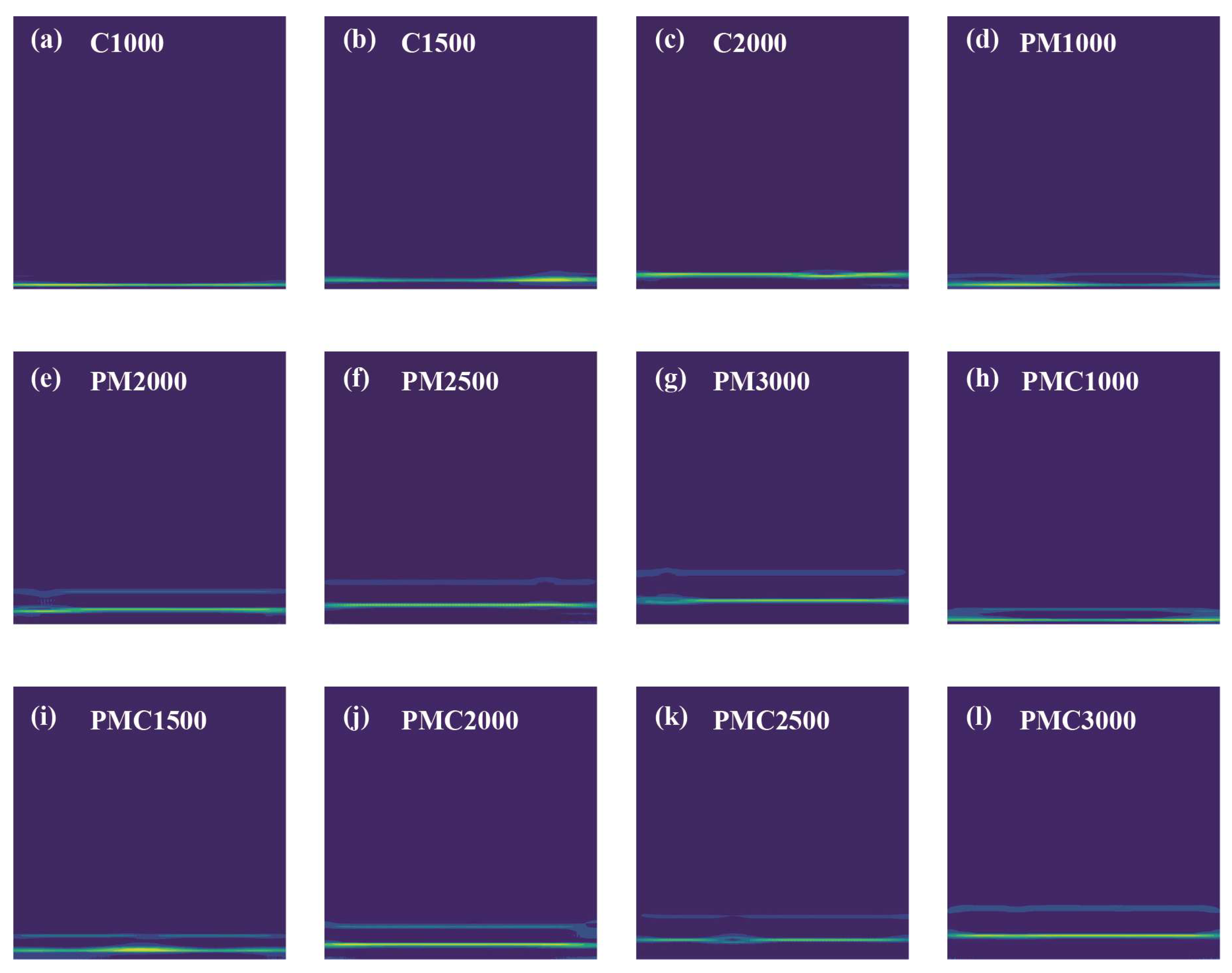
This experiment uses subsegments with a dimension of 1024 for sliding slicing to divide the original dataset into several slices. 3000 samples were selected for each state for training, and the remaining 900 samples were tested. Using the complex Morlet wavelet as the mother wavelet of CWT to obtain the time-frequency graph of each sample, the input time-frequency graph is shown in Figure 9.

The time-frequency chart shows that the characteristics of the same fault form are similar, and the signal is mainly concentrated in the low-frequency region. As the rotational speed increases, the brightness of the time-frequency graph signal increases, reflecting an increase in energy. In the time-frequency plots of PM and PMC fault types, there is a darker straight line that may correspond to the stationary part of the signal and some noise.

4.2. Analysis of Diagnostic Results from Different Models

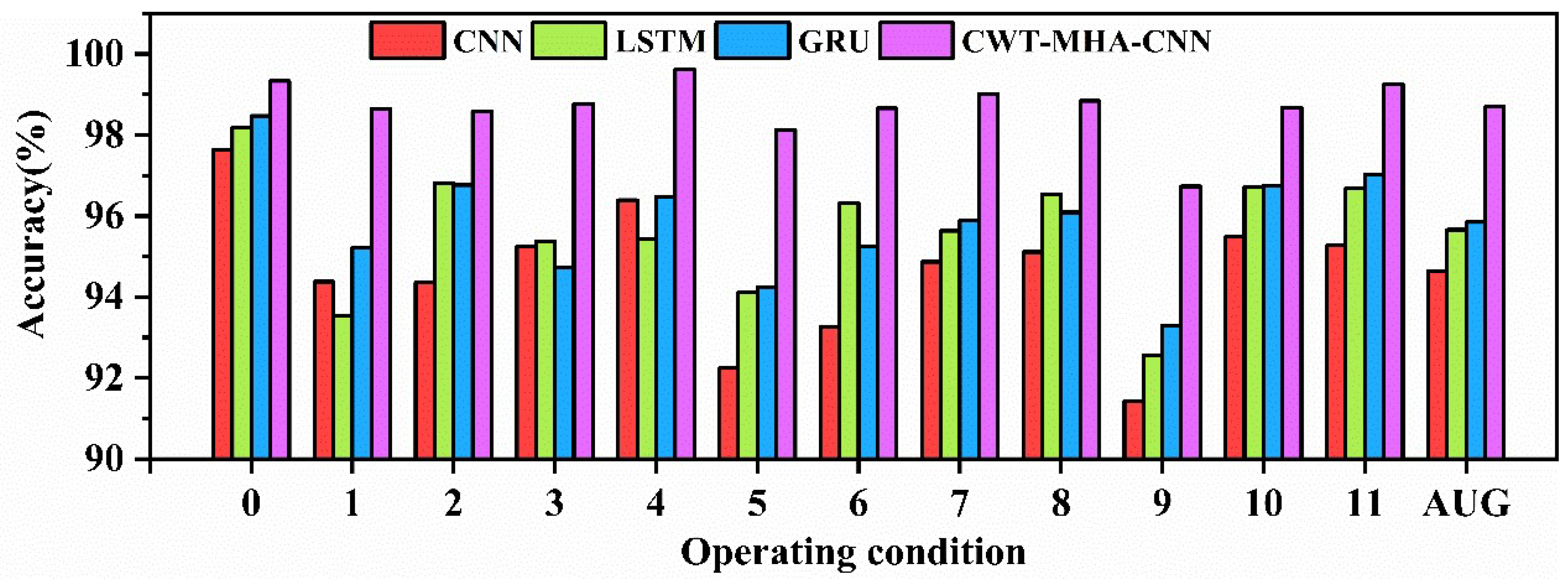
Firstly, experiments were conducted on the raw data of pump station units, and the diagnostic accuracy of different models is shown in

Table 3. Diagnostic accuracy of different models (%).

Category	CNN	LSTM	GRU	CWT-MHA-CNN
0	97.63	98.18	98.47	99.33
1	94.38	93.54	95.23	98.64
2	94.36	96.81	96.76	98.59
3	95.24	95.37	94.72	98.77
4	96.39	95.44	96.47	99.62
5	92.25	94.12	94.24	98.13
6	93.26	96.32	95.25	98.66
7	94.87	95.63	95.88	99.01
8	95.11	96.53	96.09	99.84
9	91.43	92.55	93.29	96.73
10	95.48	96.72	96.75	98.68
11	95.27	96.68	97.02	99.25
AUG	94.64	95.66	95.85	98.79

, where “AVG” represents the average accuracy. Figure 10 shows the bar charts of diagnostic results for different models.

As shown in the above chart, the average accuracy of the CNN model on pump station unit fault data is 94.64%, which is lower than other methods. This is attributed to the fixed perception field of view in the convolutional layers of CNN, which limits its ability to capture global vibration signals, makes it difficult to connect global contextual information, and is prone to getting stuck in local optima, thereby reducing accuracy. Although LSTM and GRU models have achieved certain accuracy in pump station unit fault diagnosis, with average accuracy rates of 95.66% and 95.85%, they are still insufficient compared to the CWT-MHA-CNN model proposed in this paper.

This is mainly because LSTM and GRU still have limitations in handling complex sequential dependencies, making it difficult to effectively learn and remember key information in long sequences. The reason why the CWT-MHA-CNN model can achieve higher accuracy is that it can generate time-frequency graphs by capturing signal time-frequency changes and comprehensively describing signal characteristics. Utilizing the MHA multi-head attention mechanism to associate features and temporal information enhances the concatenation of global contextual information. Finally, by combining the advantages of CNN in image recognition, we aim to improve the accuracy and efficiency of signal classification, recognition, and other tasks.

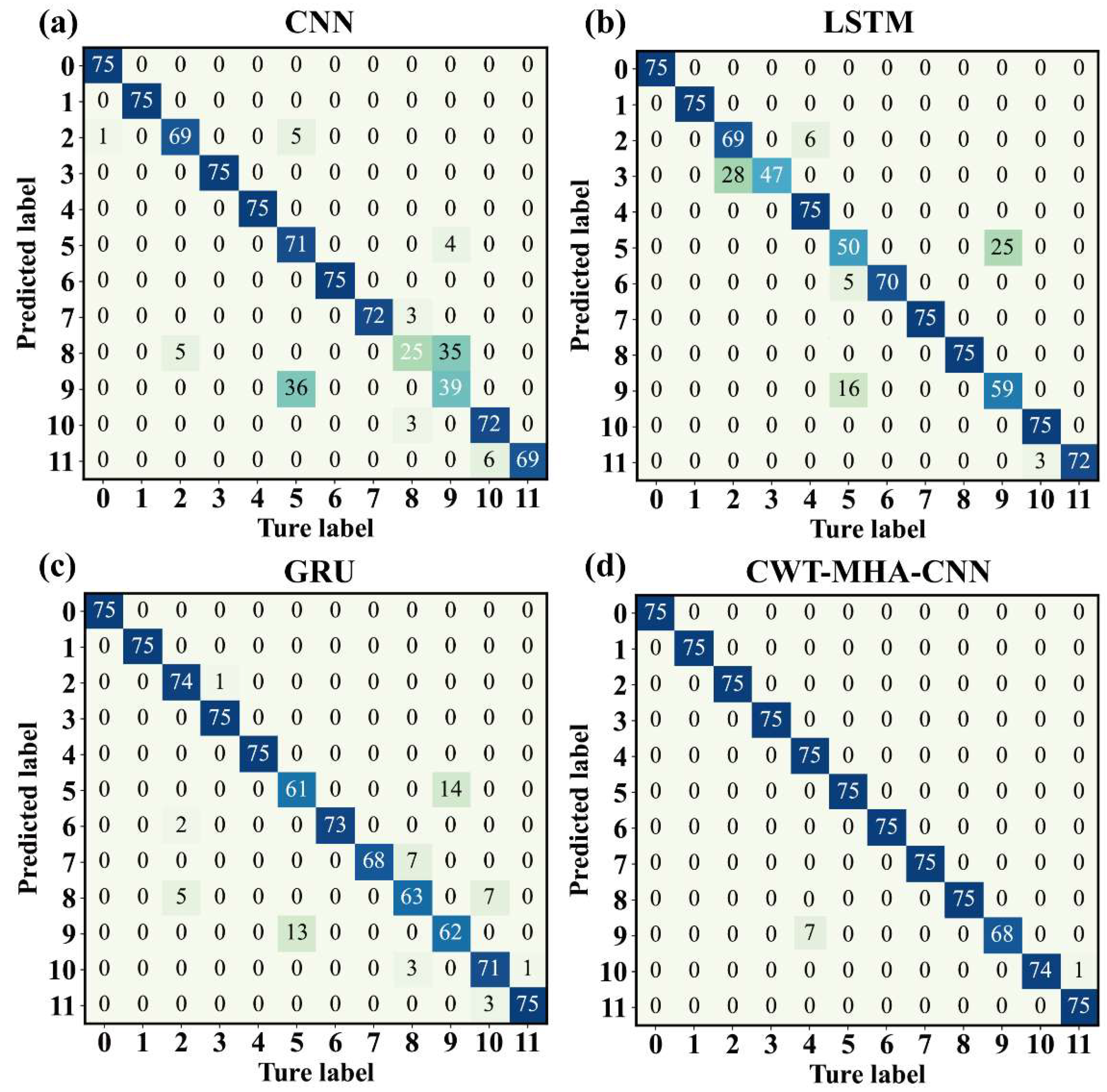
In addition, as shown in the above chart, the accuracy of operating conditions 5 and 9 is relatively low, mainly due to the highly similar amplitude and frequency characteristics of their vibration signals, making it difficult for the model to make precise distinctions. The confusion matrix in Figure 11 also reveals this issue, indicating that the model is prone to misjudging between condition 5 and condition 9 during the classification process, highlighting the limitations of the model when dealing with complex data with similar features.

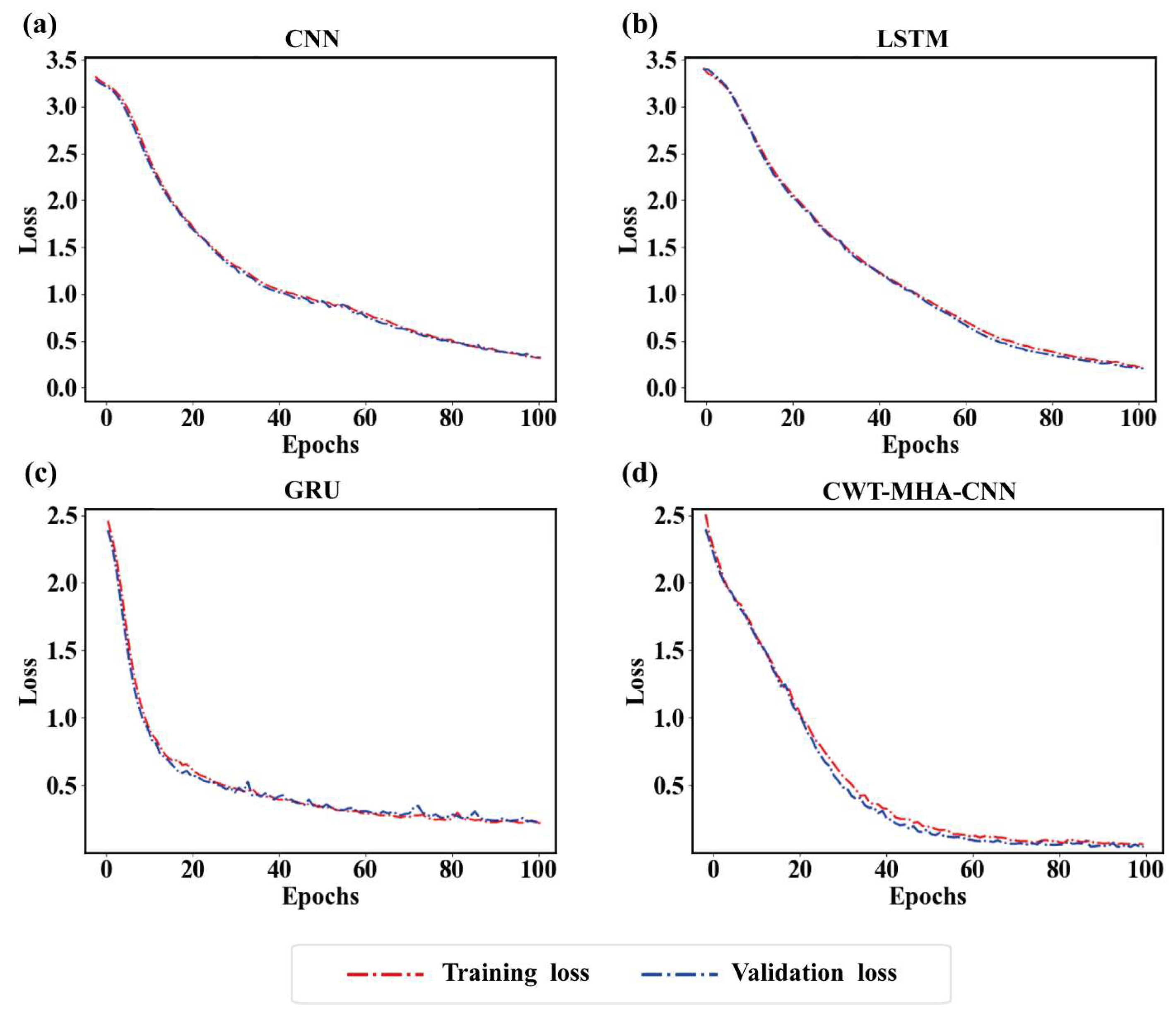
Further exploring the learning situation and performance of the training model training process, Figure 12 illustrates the changes in mean square error (loss) of the CWT-MHA-CNN model, CNN model, LSTM model, and GRU model during the training and validation processes. As the number of iterations increases, the loss on both the training and validation sets gradually decreases and tends to stabilize when the number of iterations reaches a certain value. The fewer times this stable trend occurs and the smaller the loss value, the better the convergence effect and the superior performance of the model.

As shown in the figure, the CNN model tends to stabilize after about 60 iterations, the LSTM model tends to stabilize after about 80 iterations, and both the GRU model and CWT-MHA-CNN model show a stable trend after about 40 iterations. This indicates that the GRU model and the CWT-MHA-CNN model are superior in terms of convergence speed compared to the first two. However, it is worth noting that the loss curve of the GRU model on the validation set is not completely smooth, and there is a phenomenon of local protrusions.

While the loss on the training set decreased gradually, the loss on the validation set increased, suggesting that the model may have a slight overfitting phenomenon. In contrast, the loss curve of the CWT-MHA-CNN model is relatively smooth, and there is no obvious bump, which indicates that this model is better than the other four models in terms of performance.

In summary, the CWT-MHA-CNN model has shown advantages in convergence speed and performance, and there is no obvious overfitting phenomenon, which provides strong support for its application in pump station unit fault diagnosis.

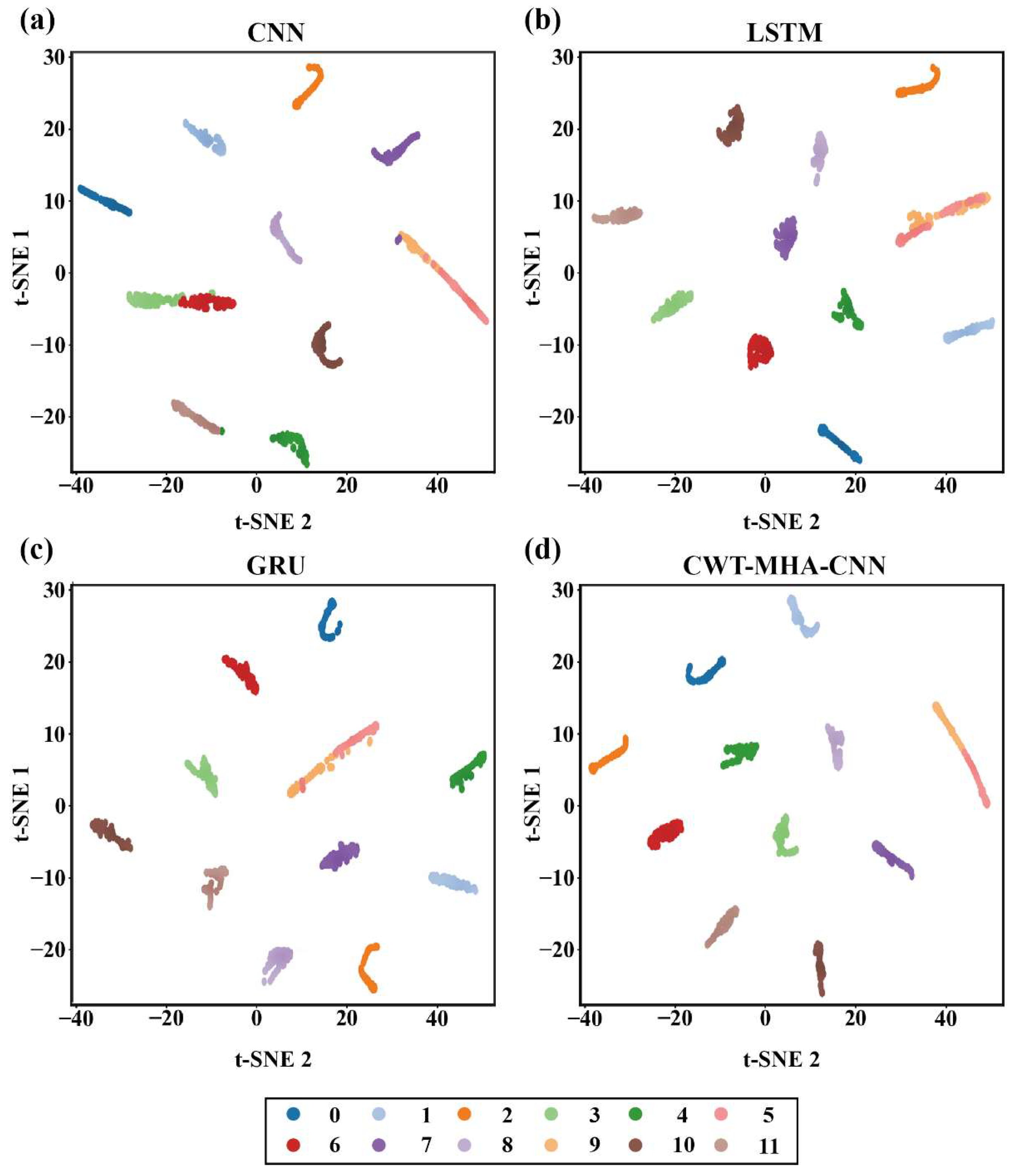
In order to better demonstrate the feature adaptation performance of the proposed method, the t-SNE algorithm was used to visualize the feature samples of different models after dimensionality reduction on the test set of pump station unit fault data, as shown in Figure 13.

Through the visualization of t-SNE dimensionality reduction, it can be seen that the CWT-MHA-CNN model has a more compact intraclass clustering and a more distinct interclass distribution compared to the CNN model, LSTM model, and GRU model. All four models can better identify other working conditions, except for working conditions 5 and 9. However, there is some overlap in identifying events in working conditions 5 and 9, and the effect is not significant compared to other working conditions. This is consistent with the results of the confusion matrix in Figure 11. Based on the qualitative analysis of the above visualization, this article also selected the interclass distance based on data labels for quantitative evaluation, as shown in

Table 4. Comparison of performance indicators of different models.

Model	NMI	DBI	SIL
CNN	0.832	0.21	0.814
LSTM	0.867	0.14	0.873
GRU	0.885	0.11	0.882
CWT-MHA-CNN	0.928	0.04	0.917

. Standardized Mutual Information (NMI), as an external indicator for evaluating clustering performance, is used to measure the degree of conformity between clustered data labels and real labels. The closer its value is to 1, the better the clustering effect. The NMI index of the CWT-MHA-CNN model is 0.92, and the Davidson Boding index (DBI) is an internal indicator for evaluating clustering performance. A smaller value indicates higher clustering effectiveness and lower dispersion. The DBI value of the CWT-MHA-CNN model is 0.04; the closer the silhouette coefficient (SIL) approaches 1, the better the cohesion and separation. The SIL value of the CWT-MHA-CNN model is 0.917. Overall, the CWT-MHA-CNN proposed in this article outperforms other models in terms of performance.

4.3. Analysis of Diagnostic Results of Different Models for Noisy Fault Samples

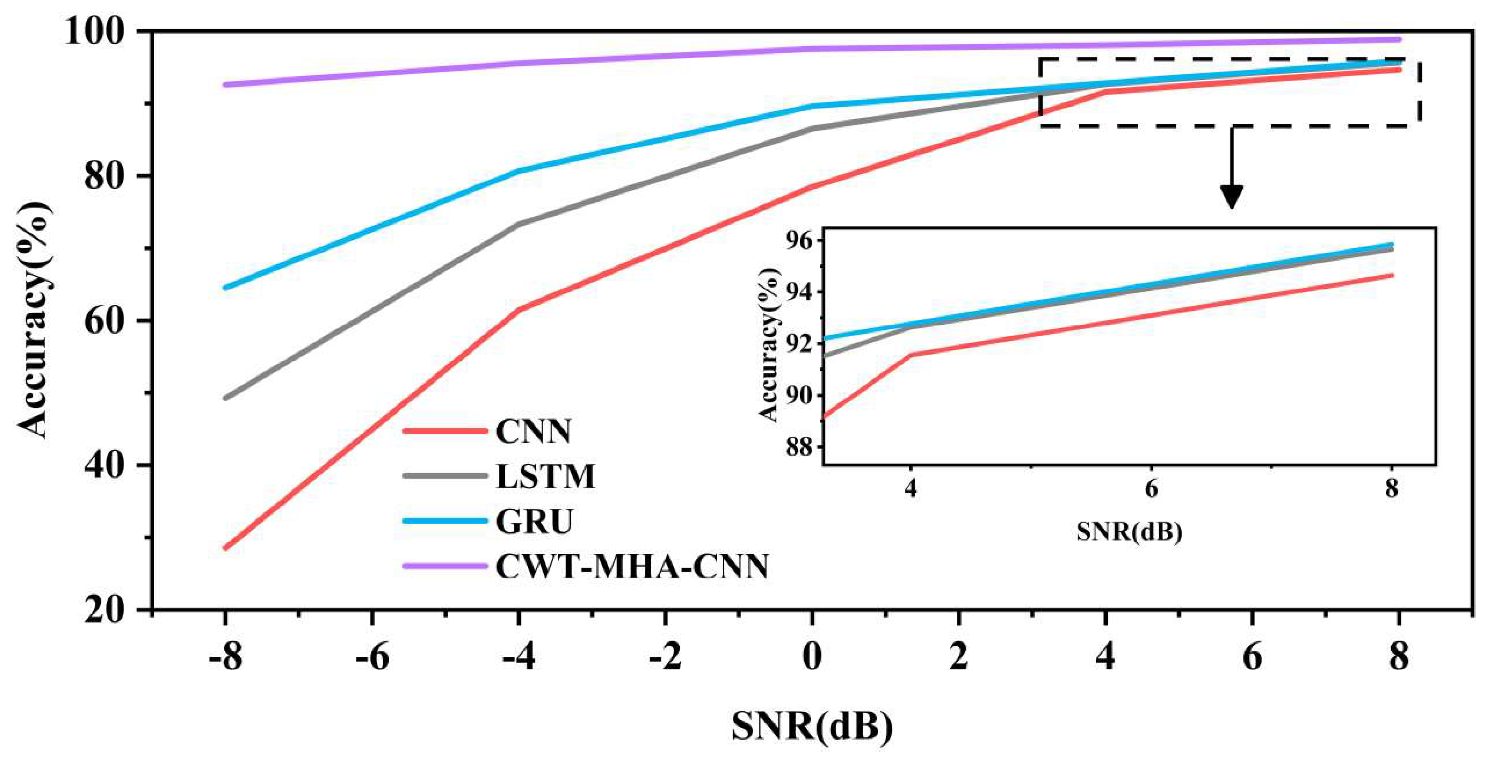
In order to explore the noise resistance performance of the CWT-MHA-CNN model proposed in this article, training tests were conducted using noisy fault sample signals constructed in Section 3.2, ranging from −8 dB to 8 dB. The diagnostic results were then compared with those of the CNN model, the LSTM model, and the GRU model. For each model, the average result of 10 experiments was used as the evaluation criterion, and the specific results are shown in

Table 5. Average accuracy of different models under different noise environments.

Accuracy	SNR (dB)
	−8	−6	−4	−2	0	2	4	6	8
CNN	32.53	42.93	51.42	64.23	73.44	80.25	88.56	91.32	94.32
LSTM	54.26	61.53	73.26	79.21	86.51	88.69	91.63	93.45	95.36
GRU	63.53	75.25	81.64	85.57	89.63	91.22	92.77	94.27	95.17
MHA-CWT-CNN	92.54	94.97	95.54	96.13	97.51	97.61	98.02	98.53	98.73

. Figure 14 shows the trend of accuracy changes better in line graphs with different model accuracies.

According to the chart analysis, when the signal-to-noise ratio (SNR) is greater than 4 dB, the accuracy of all four models shows a high level. However, when the signal-to-noise ratio is in the range of 0 dB to 4 dB, the accuracy of the CNN model significantly decreases, while the other three models still maintain high accuracy. Specifically, when the SNR drops below 0 dB, the accuracy of the LSTM and GRU models also begins to show a significant downward trend. It is worth noting that the CWT-MHA-CNN model can still maintain an accuracy of 97.51% even at an SNR of 0 dB, demonstrating its stability in lower signal-to-noise ratio environments. Furthermore, in a strong noise environment (SNR = 8 dB), the accuracy of the other three comparison models is relatively low, while the CWT-MHA-CNN model can still maintain high accuracy, indicating its strong ability to resist noise.

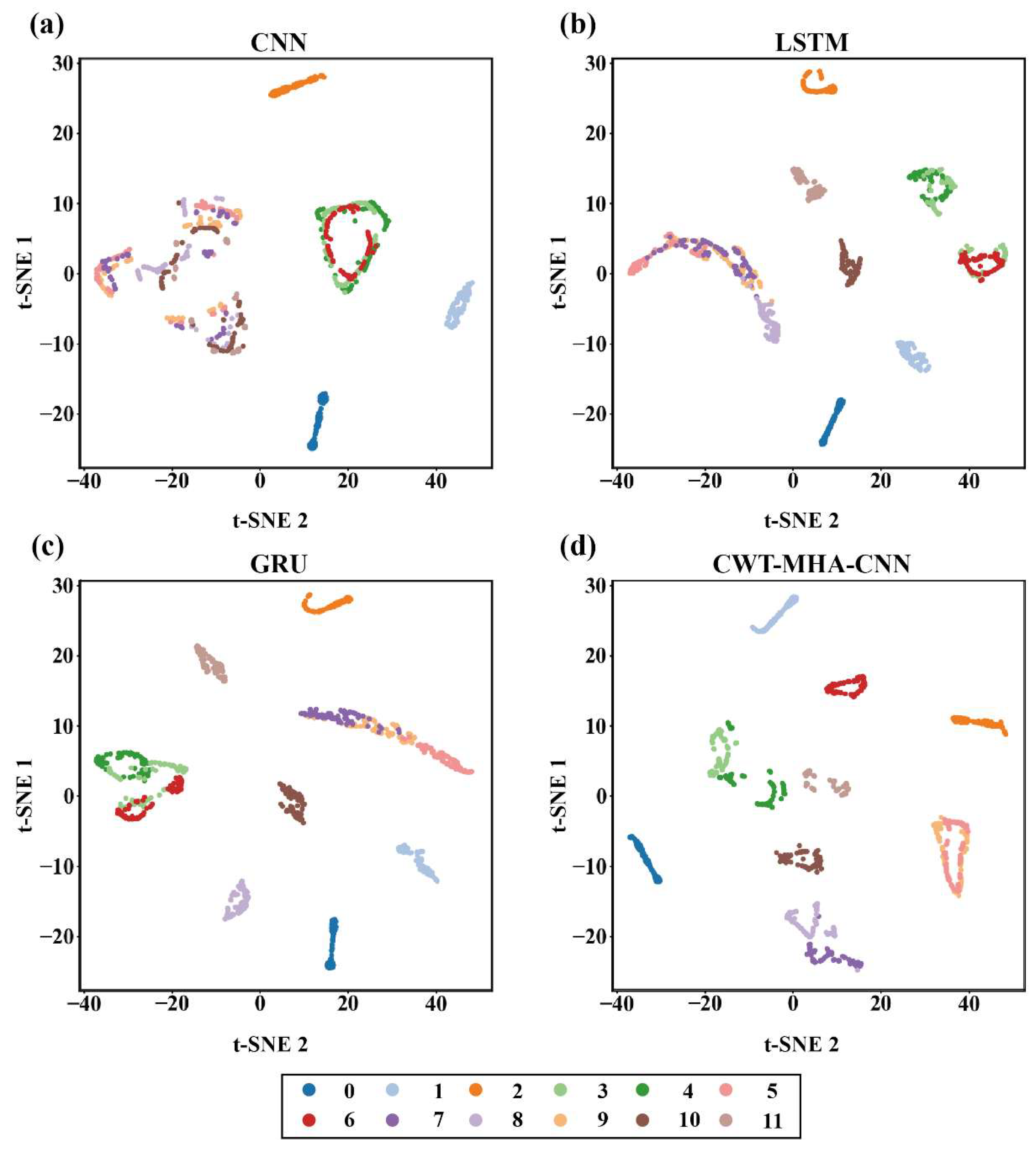
In order to further analyze the classification performance and explain the reason why the CWT-MHA-CNN model performs better, we generated t-SNE dimensionality reduction visualizations of CNN, LSTM, GRU, and CWT-MHA-CNN in a noisy environment of −8 dB, as shown in Figure 15.

In a strong noise environment with an SNR of −8 dB, the interclass distance significantly increases compared to the non-noise condition, especially for working conditions 3, 4, 5, 6, 7, 8, and 9. In this environment, the clustering and classification ability of CNN models is the worst, and their clustering performance is particularly poor for working conditions 7, 8, 9, 10, and 11. The data points for these working conditions mostly overlap, leading to difficulties in intraclass clustering and interclass separation. At the same time, working conditions 4, 5, and 6 also have similar problems, which are mainly attributed to the insufficient noise resistance performance of CNN, making it difficult to effectively extract discriminative features from noisy and similar signals.

The LSTM model and GRU model also face challenges in distinguishing between operating conditions 4, 5, and 6, as well as operating conditions 3, 7, 8, and 9, where the data points overlap severely. After analysis, working conditions 4, 5, and 6 exhibit high similarity in their characteristics due to the same fault coming from different speeds. However, working conditions 3, 7, 8, and 9 have similar frequencies, resulting in overlapping energy distributions at the same scale and position, which increases the difficulty of distinguishing between LSTM and GRU.

In contrast, the CWT-MHA-CNN model proposed in this article, although there is a certain degree of overlap in the clustering of operating conditions 3 and 7, maintains a relatively tight intraclass spacing for other operating conditions and a relatively distant interclass distribution. Overall, the CWT-MHA-CNN model exhibits better clustering performance in strong noise environments compared to the other three models, demonstrating its strong ability to resist noise and extract features.

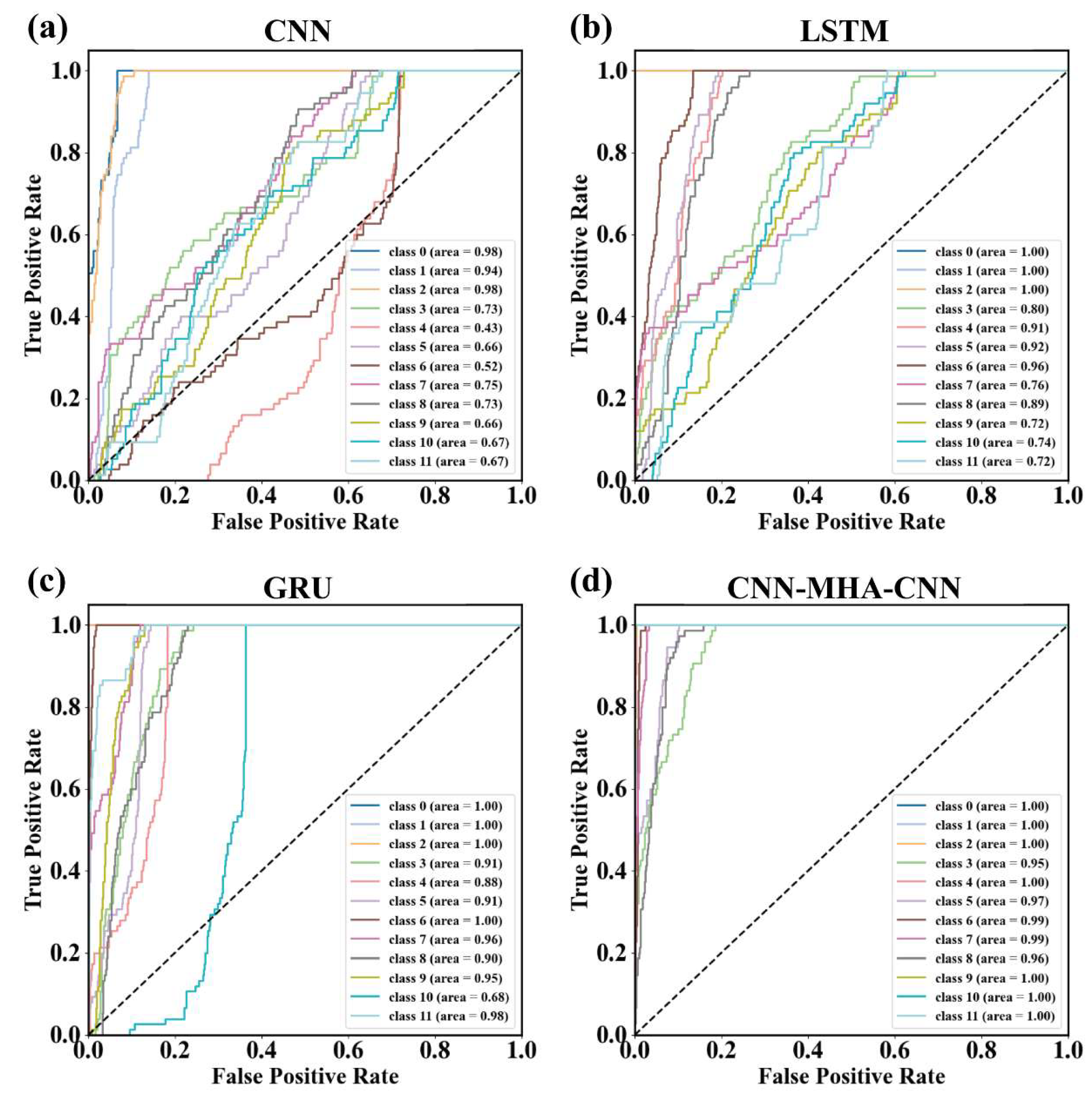
In the previous analysis, we fully demonstrated the excellent performance of the CWT-MHA-CNN model in terms of noise resistance through accuracy calculation and t-SNE dimensionality reduction visualization. In order to comprehensively and deeply evaluate the performance of the model, we further introduced the ROC curve as an important evaluation tool. The ROC curve, also known as the receiver operating characteristic curve, provides a comprehensive and detailed perspective to examine the classification performance of the model by depicting the relationship between true case rate (TPR) and false positive case rate (FPR) under different classification thresholds. It not only intuitively reflects the stability of the model in different noise environments but also reveals the balance of the model’s ability to identify positive and negative examples, which helps us to analyze the model’s performance more deeply. Figure 16 shows the comparison of ROC curves for four models: CNN, LSTM, GRU, and CWT-MHA-CNN.

From the graph, it can be observed that the ROC curve of the CWT-MHA-CNN model is closer to the upper left corner compared to the other three models, indicating that its area under the curve (AUC) is the largest. As an indicator for evaluating the overall performance of a model, the larger the AUC, the better the performance of the model under different classification thresholds, indicating a higher ability of the model to identify true cases. In addition, the slope of the ROC curve of CWT-MHA-CNN is the highest, which reflects the rate of change in true and false positive rates under different classification thresholds. The larger the slope, the more significant the change in model performance with threshold, further reflecting the stability and sensitivity of the CWT-MHA-CNN model in classification tasks.

4.4. Failure Mode Analysis

To observe the learnt fault patterns, we visualized the mixed information and assigned weights of the multi-head attention mechanism (MHA) of the proposed CWT-MHA-CNN model, along with the outputs of the CNN model’s Conv2d_1, Conv2d_2 layers, Dense1, and Dense2 layers. A sample of fault is chosen from the test set. Then we use the trained CWT-MHA-CNN model to predict the fault sample.

Firstly, we select a fault sample that belongs to operating condition 4 as the sample and then convert it into a time-frequency graph through CWT, as shown in Figure 17.

The multi-head attention mechanism can extract more correlated information by correlating input information and variables, thereby reducing the risk of overfitting that may occur with a single attention head. Meanwhile, through the joint learning of multiple attention heads, this mechanism effectively improves the generalization performance of the model.

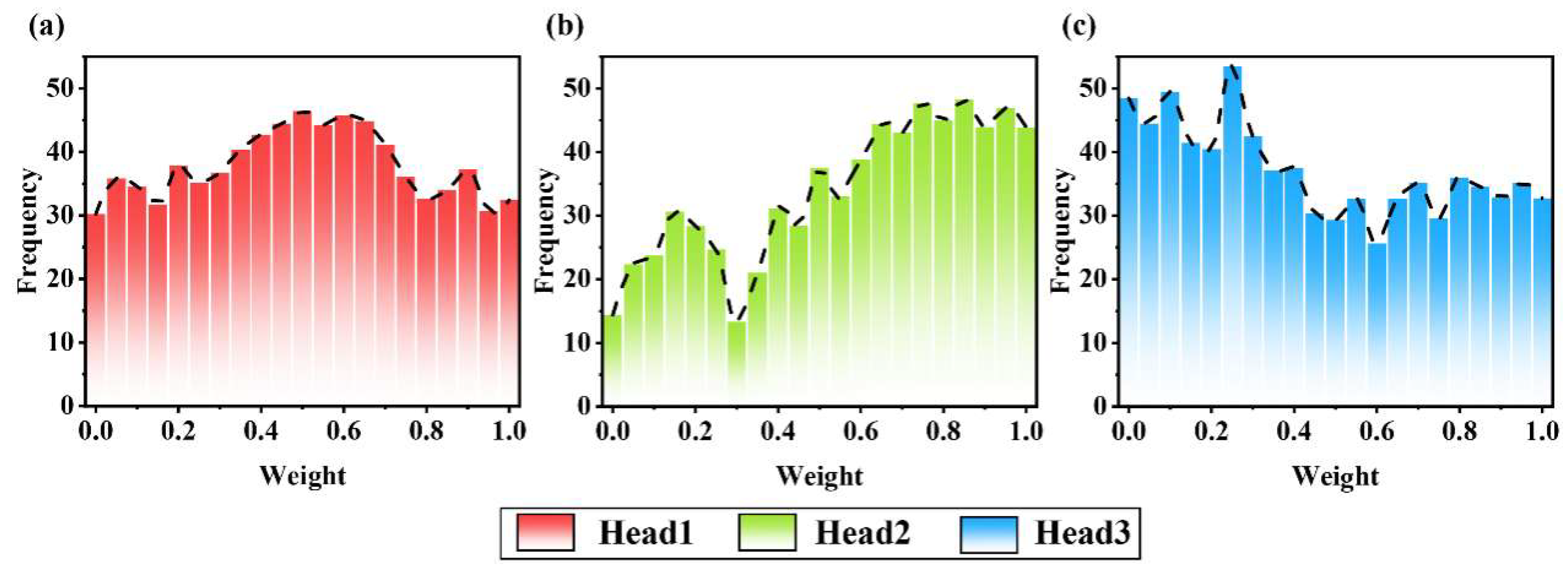
In order to further explore the working principle of the multi-head attention mechanism, we applied it to input data and visualized the mixed information and weights of different channels, as shown in Figure 18. From the graph, it can be observed that the sensitivity of different attention heads (heads) in the multi-head attention mechanism (MHA) to vibration signal data varies: Head1 is more sensitive to vibration signals in the middle region, Head2 shows higher sensitivity to vibration signals in the high-frequency region, and Head3 is better at processing vibration signals in the low-frequency region. These results not only validate the effectiveness of the multi-head attention mechanism in extracting complex signal features but also provide valuable clues for us to deeply understand its working mechanism.

To verify the attention mechanism of MHA in processing variance information, we input faulty sample data into MHA and extracted the weights of the sample information. Figure 19 shows the weight distribution histograms of Head1, Head2, and Head3. Observing Figure 19, we found that the weight distribution of Head1 exhibits a normal distribution, which reflects its upward and downward role in task processing. It receives information from the early stages and provides effective feature representations for task processing in the later stages, so it needs to focus more on fine processing and analysis of information in the middle stage. Head2 allocates relatively small weights in the early stages of training but gradually increases in the later stages, reflecting the model’s handling of input information diversity in the adaptation stage. As the training progresses, the model gradually learns to filter out feature information that is more critical to the task from the input and increases its attention to this information, resulting in an increase in attention weights in the later stage. In contrast, Head3 is assigned a larger weight in the early stages, indicating that Head1 focuses more on the feature information that contributes significantly to the task in the early stages of training, playing a crucial role in the model’s understanding and prediction in the initial stage.

Overall, the model dynamically adjusts the weights of different attention heads to adapt to the diversity and complexity of input information, thereby optimizing its performance on specific tasks. This adjustment reflects the learning and adaptability of the model during the training process, enabling it to gradually focus on more critical feature information for the task.

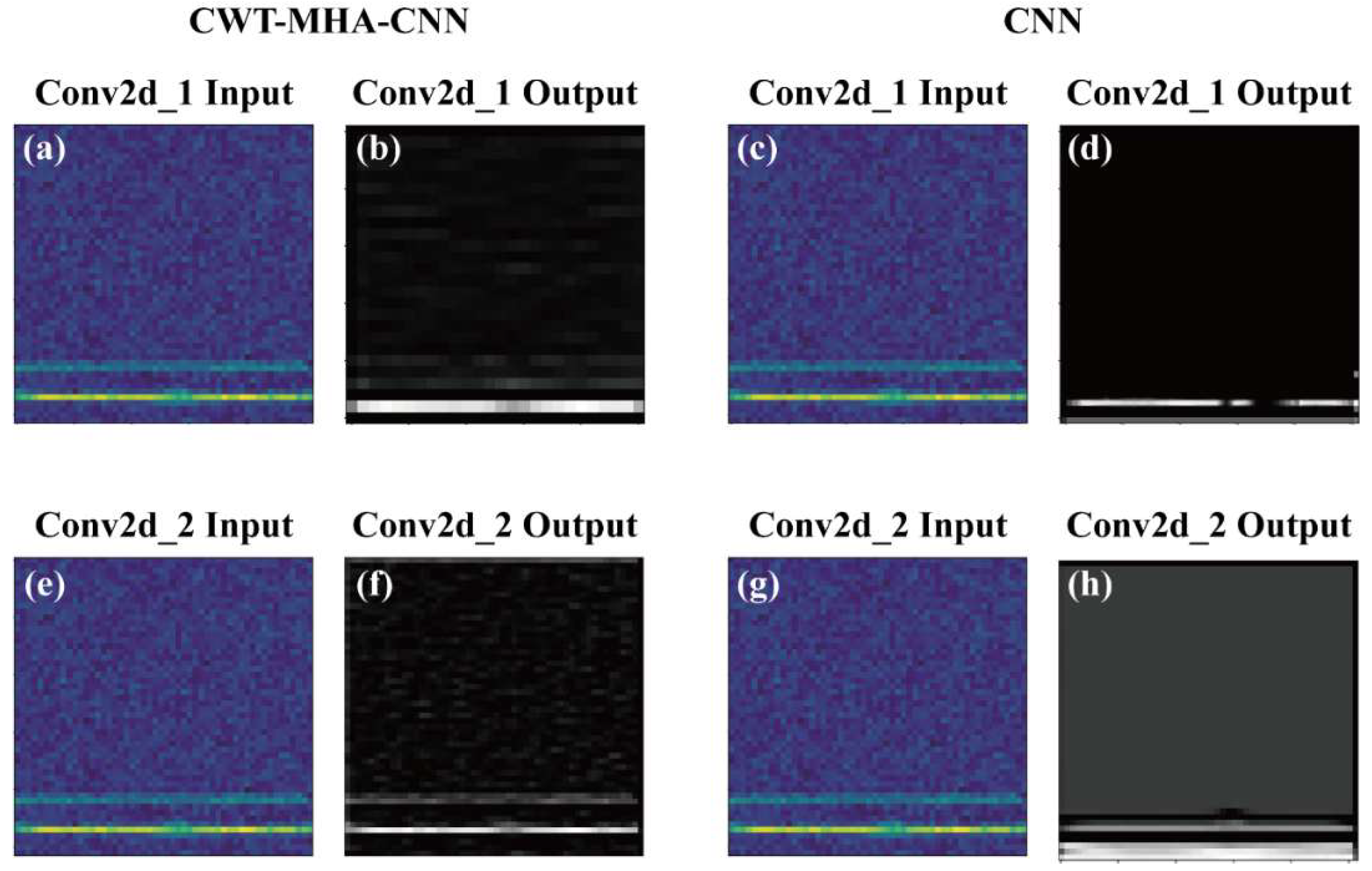
Next, in order to further explore the feature extraction capability of CNN models, we conducted visual analysis on the Conv2d_1 and Conv2d_2 layers in CNN, as shown in Figure 20. From the figure, it can be observed that the Conv2d_1 layer is able to extract edge and texture information from the image in the sample. However, due to the fact that the Conv2d_1 layer is a shallow convolutional layer, there are still certain limitations in extracting detailed features. As the number of network layers deepens, clear feature representations can already be extracted when reaching the Conv2d_2 layer. Further observation reveals that the features extracted by the Conv2d_2 layer in the samples are basically consistent with those in the labels. At the same time, in order to verify the effectiveness of the CWT-MHA-CNN model in identifying fault patterns, we tested the same sample using a trained CNN model and the CWT-MHA-CNN model and conducted a visual comparison. From the figure, it can be observed that the features extracted by the CNN model in the Conv2d_1 layer are relatively fuzzy and incomplete, while the similarity between the features extracted in the Conv2d_2 layer and the original label is also low. The inaccuracy and incompleteness of this feature extraction may be detrimental to the accurate judgment of the model. In contrast, the CWT-MHA-CNN model exhibits higher clarity and completeness in feature extraction at the same level and also has a higher matching degree with the original label. In summary, these results validate the effectiveness of the CWT-MHA-CNN model in fault recognition tasks and demonstrate its powerful feature extraction ability.

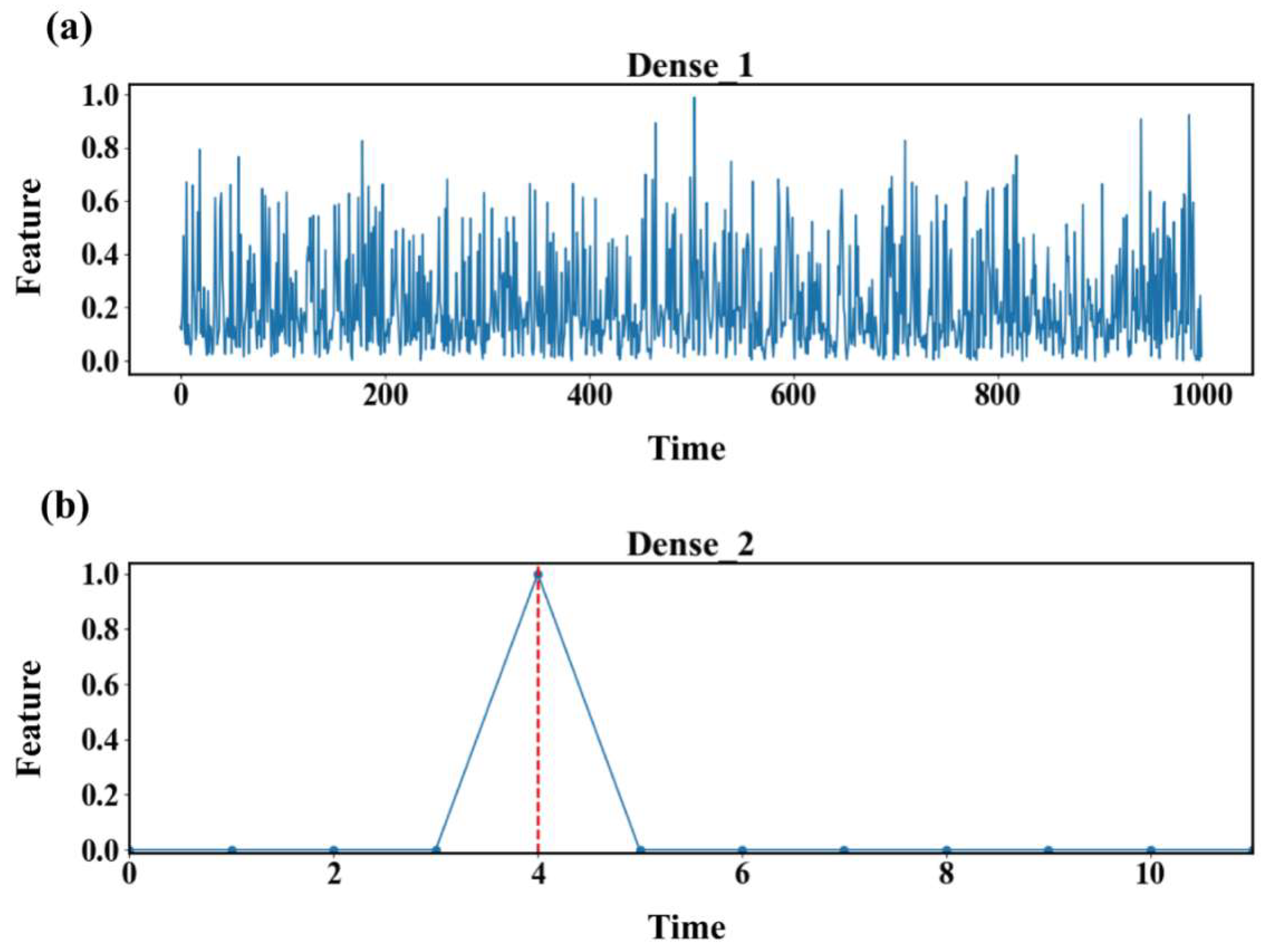
The features extracted from the Conv2d_2 layer are flattened through the Dense1 layer to convert the data from two-dimensional images into one-dimensional vectors, and these features are used for the final classification task. The Dense2 layer outputs the classification results of fault samples, as shown in Figure 21. The abscissa corresponding to the peak value of the curve in Figure 21b is considered the result of a fault diagnosis. We can see that the fault diagnosis results are consistent with their labels, verifying the effectiveness of the identified fault mode.

5. Conclusions

This study presents a deep learning-driven fault diagnosis approach for pumping station units, integrating continuous wavelet transform (CWT) with a multi-head attention convolutional neural network (MHA-CNN). Initially, time-domain signals are transformed into time-frequency representations using CWT to extract their time-frequency features. Subsequently, the MHA mechanism synthesises these features alongside temporal delay data, improving the model’s capacity to identify critical information and temporal dependencies. The aggregated features are then processed by a convolutional neural network (CNN) to generate precise fault classification. The proposed method exhibits notable efficiency and robustness in diagnosing pumping station unit faults, accommodating diverse operational scenarios and noise disturbances, thereby ensuring reliable performance in real-world implementations. Specifically:

(1)

During the training of the original fault samples, the CWT-MHA-CNN model proposed in this paper demonstrated excellent performance, with an average accuracy of 98.79%. It is worth noting that the model also achieved satisfactory performance in distinguishing between operating conditions 5 and 9 with similar features, which further confirms its strong classification ability. In addition, by using t-SNE dimensionality reduction visualization technology, we observed that the CWT-MHA-CNN model has excellent clustering performance, which provides strong support for its stability and reliability in practical applications.

(2)

The CWT-MHA-CNN model has demonstrated excellent noise resistance. When diagnosing noisy fault signals with a signal-to-noise ratio of −8 to 8 dB, we observed that the accuracy of the CWT-MHA-CNN model was 92.54%, 94.97%, 95.54%, 96.13%, 97.51%, 97.61%, 98.02%, 98.53%, and 98.73%, respectively. This series of accuracy data fully proves that the diagnostic method proposed in this article can still maintain stable and reliable performance in the actual operating environment of pumping station units. Even in situations with severe noise interference, the CWT-MHA-CNN model can still accurately identify fault signals. This ensures that the diagnostic method proposed in this article remains stable and reliable in the actual operation of pumping station units.

(3)

The effectiveness and superiority of the CWT-MHA-CNN model in fault mode analysis were demonstrated by visualizing the MHA and Conv2d_1, Conv2d_2, Dense1, and Dense2 layers during the training process of fault samples belonging to condition 4 using CWT-MHA-CNN. This provides a reference for effectively constructing diagnostic models for pump station units and is of great significance for ensuring the safe operation of pump station units.

References

1. Zhao, Y.P.; Zhang, P.L.; Pu, Y.J.; Lei, H.; Zheng, X.B. Unit Operation Combination and Flow Distribution Scheme of Water Pump Station System Based on Genetic Algorithm. Appl. Sci. 2023, 13, 11869. [Google Scholar] [CrossRef]
2. Lei, Y.G.; Yang, B.; Jiang, X.W.; Jia, F.; Li, N.P.; Nandi, A.K. Applications of machine learning to machine fault diagnosis: A review and roadmap. Mech. Syst. Signal Process. 2020, 138, 106587. [Google Scholar] [CrossRef]
3. Milošević, M.; Radić, M.; Rašić-Amon, M.; Litričin, D.; Stajić, Z. Diagnostics and control of pumping stations in water supply systems: Hybrid model for fault operating modes. Processes 2022, 10, 1475. [Google Scholar] [CrossRef]
4. Hoang, D.-T.; Kang, H.-J. A survey on deep learning based bearing fault diagnosis. Neurocomputing 2019, 335, 327–335. [Google Scholar] [CrossRef]
5. Zarei, J.; Tajeddini, M.A.; Karimi, H.R. Vibration analysis for bearing fault detection and classification using an intelligent filter. Mechatronics 2014, 24, 151–157. [Google Scholar] [CrossRef]
6. Chacon, J.L.F.; Kappatos, V.; Balachandran, W.; Gan, T.-H. A novel approach for incipient defect detection in rolling bearings using acoustic emission technique. Appl. Acoust. 2015, 89, 88–100. [Google Scholar] [CrossRef]
7. Singh, S.; Kumar, A.; Kumar, N. Motor current signature analysis for bearing fault detection in mechanical systems. Procedia Mater. Sci. 2014, 6, 171–177. [Google Scholar] [CrossRef]
8. Zhao, Z.-Q.; Huang, D.-S.; Sun, B.-Y. Human face recognition based on multi-features using neural networks committee. Pattern Recognit. Lett. 2004, 25, 1351–1358. [Google Scholar] [CrossRef]
9. Li, Y.B.; Xu, M.Q.; Wei, Y.; Huang, W.H. A new rolling bearing fault diagnosis method based on multiscale permutation entropy and improved support vector machine based binary tree. Measurement 2016, 77, 80–94. [Google Scholar] [CrossRef]
10. Li, C.; Sanchez, R.-V.; Zurita, G.; Cerrada, M.; Cabrera, D.; Vásquez, R.E. Multimodal deep support vector classification with homologous features and its application to gearbox fault diagnosis. Neurocomputing 2015, 168, 119–127. [Google Scholar] [CrossRef]
11. Jia, F.; Lei, Y.G.; Lin, J.; Zhou, X.; Lu, N. Deep neural networks: A promising tool for fault characteristic mining and intelligent diagnosis of rotating machinery with massive data. Mech. Syst. Signal Process. 2016, 72, 303–315. [Google Scholar] [CrossRef]
12. Hinton, G.E.; Salakhutdinov, R.R. Reducing the dimensionality of data with neural networks. Science 2006, 313, 504–507. [Google Scholar] [CrossRef] [PubMed]
13. Deng, L.; Yu, D. Deep learning: Methods and applications. Found. Trends® Signal Process. 2014, 7, 197–387. [Google Scholar] [CrossRef]
14. Hinton, G.; Deng, L.; Yu, D.; Dahl, G.; Mohamed, A.-R.; Jaitly, N.; Senior, A.; Vanhoucke, V.; Nguyen, P.; Sainath, T.; et al. Deep neural networks for acoustic modeling in speech recognition: The shared views of four research groups. IEEE Signal Process. Mag. 2012, 29, 82–97. [Google Scholar] [CrossRef]
15. Krizhevsky, A.; Sutskever, I.; Hinton, G.E. Imagenet classification with deep convolutional neural networks. Cmmunications ACM 2017, 60, 84–90. [Google Scholar] [CrossRef]
16. LeCun, Y.; Boser, B.; Denker, J.S.; Henderson, D.; Howard, R.E.; Hubbard, W.; Jackdl, L.D. Backpropagation applied to handwritten zip code recognition. Neural Comput. 1989, 1, 541–551. [Google Scholar] [CrossRef]
17. Simonyan, K.; Zisserman, A. Very deep convolutional networks for large-scale image Recognition. arXiv 2014, arXiv:1409.1556. [Google Scholar]
18. LeCun, Y.; Bengio, Y.; Hinton, G. Deep learning. Nature 2015, 521, 436–444. [Google Scholar] [CrossRef]
19. Eren, L.; Ince, T.; Kiranyaz, S. A generic intelligent bearing fault diagnosis system using compact adaptive 1D CNN classifier. J. Signal Process. Syst. 2019, 91, 179–189. [Google Scholar] [CrossRef]
20. Shuuji, M.; Song, X.; Liao, Z.; Chen, P. Low-speed bearing fault diagnosis based on improved statistical filtering and convolutional neural network. Meas. Sci. Technol. 2021, 32, 115009. [Google Scholar] [CrossRef]
21. Wang, D.C.; Guo, Q.W.; Song, Y.; Gao, S.Y.; Li, Y.B. Application of multiscale learning neural network based on CNN in bearing fault diagnosis. J. Signal Process. Syst. 2019, 91, 1205–1217. [Google Scholar] [CrossRef]
22. Wang, H.; Xu, J.W.; Yan, R.Q.; Gao, R.X. A new intelligent bearing fault diagnosis method using SDP representation and SE-CNN. IEEE Trans. Instrum. Meas. 2019, 69, 2377–2389. [Google Scholar] [CrossRef]
23. Liu, C.-L.; Hsaio, W.-H.; Tu, Y.-C. Time series classification with multivariate convolutional neural network. IEEE Trans. Ind. Electron. 2018, 66, 4788–4797. [Google Scholar] [CrossRef]
24. Wen, L.; Li, X.Y.; Gao, L.; Zhang, Y.Y. A new convolutional neural network-based data-driven fault diagnosis method. IEEE Trans. Ind. Electron. 2017, 65, 5990–5998. [Google Scholar] [CrossRef]
25. Hochreiter, S.; Bengio, Y.; Frasconi, P.; Schmidhuber, J. Gradient flow in recurrent nets: The difficulty of learning long-term dependencies. Field Guide Dyn. Recurr. Neural Netw. 2001, 237–243. [Google Scholar] [CrossRef]
26. Zhuang, F.Z.; Qi, Z.Y.; Duan, K.Y.; Xi, D.B.; Zhu, Y.C.; Zhu, H.S.; Xiong, H.; He, Q. A comprehensive survey on transfer learning. Proc. IEEE 2020, 109, 43–76. [Google Scholar] [CrossRef]
27. Xu, H.; Fan, F.; Zhang, H.; Le, Z.L.; Huang, J. A deep model for multi-focus image fusion based on gradients and connected regions. IEEE Access 2020, 8, 26316–26327. [Google Scholar] [CrossRef]
28. Janssens, O.; Slavkovikj, V.; Vervisch, B.; Stockman, K.; Loccufier, M.; Verstock, S.; Walle, R.V.D.; Hoecke, S.V. Convolutional neural network based fault detection for rotating machinery. J. Sound Vib. 2016, 377, 331–345. [Google Scholar] [CrossRef]
29. Feng, P.; Liang, M.; Chu, F.L. Recent advances in time–frequency analysis methods for machinery fault diagnosis: A review with application examples. Mech. Syst. Signal Process. 2013, 38, 165–205. [Google Scholar] [CrossRef]
30. Goupillaud, P.; Grossmann, A.; Morlet, J. Cycle-octave and related transforms in seismic signal analysis. Geoexploration 1984, 23, 85–102. [Google Scholar] [CrossRef]
31. Zhang, X.; Liu, Z.W.; Wang, J.X.; Wang, J.L. Time–frequency analysis for bearing fault diagnosis using multiple Q-factor Gabor wavelets. ISA Trans. 2019, 87, 225–234. [Google Scholar] [CrossRef]
32. Guo, M.-F.; Zeng, X.-D.; Chen, D.-Y.; Yang, N.-C. Deep-learning-based earth fault detection using continuous wavelet transform and convolutional neural network in resonant grounding distribution systems. IEEE Sens. J. 2017, 18, 1291–1300. [Google Scholar] [CrossRef]
33. Hu, J.; Shen, L.; Sun, G.; Albanie, S.; Wu, E. Squeeze-and-Excitation Networks. In Proceedings of the IEEE Conference on Computer Vision and Pattern Recognition (CVPR), Salt Lake City, UT, USA, 23 June 2018; pp. 7132–7141. [Google Scholar]
34. Zhou, Q.; Li, Y.B.; Tian, Y.; Jiang, L. A novel method based on nonlinear auto-regression neural network and convolutional neural network for imbalanced fault diagnosis of rotating machinery. Measurement 2020, 161, 107880. [Google Scholar] [CrossRef]
35. Jing, L.Y.; Zhao, M.; Li, P.; Xu, X.Q. A convolutional neural network based feature learning and fault diagnosis method for the condition monitoring of gearbox. Measurement 2017, 111, 1–10. [Google Scholar] [CrossRef]
36. Vaswani, A.; Shazeer, N.; Parmar, N.; Uszkoreit, J.; Jones, L.; Gomez, A.N.; Kaisier, L.; Polosukin, I. Attention is all you need. Adv. Neural Inf. Process. Syst. 2017, 30, 5998–6008. [Google Scholar]
Figure 1. Structure of SE attention mechanism.
Sustainability 17 11383 g001
Figure 2. Improve CNN Architecture.
Sustainability 17 11383 g002
Figure 3. Multi head attention mechanism.
Sustainability 17 11383 g003
Figure 4. MHA processes the data flow.
Sustainability 17 11383 g004
Figure 5. CWT-MHA-CNN fault diagnosis flow.
Sustainability 17 11383 g005
Figure 6. Schematic diagram of pump station unit experimental platform.
Sustainability 17 11383 g006
Figure 7. Fault sample construction.
Sustainability 17 11383 g007
Figure 8. Construction of noisy signals.
Sustainability 17 11383 g008
Figure 9. Time frequency plots under different operating conditions.
Sustainability 17 11383 g009
Figure 10. Diagnostic Results Bar Chart.
Sustainability 17 11383 g010
Figure 11. Confusion matrix diagrams for different models. ((a) is the confusion matrix of CNN model, (b) is the confusion matrix of LSTM model, (c) is the confusion matrix of GRU model, and (d) is the CWT-MHA-CNN model confusion matrix).
Sustainability 17 11383 g011
Figure 12. Loss curves of different models. ((a) is the Loss graph of the CNN model, (b) is the Loss graph of the LSTM model, (c) is the Loss graph of the GRU model, (d) is the Loss graph of the CWT-MHA-CNN model).
Sustainability 17 11383 g012
Figure 13. Feature distribution maps of different models. ((a) is the t-SNE graph of the CNN model, (b) is the t-SNE graph of the LSTM model, (c) is the t-SNE graph of the GRU model, and (d) is the t-SNE graph of the CWT-MHA-CNN model).
Sustainability 17 11383 g013
Figure 14. Classification accuracy of different methods under different noise environments.
Sustainability 17 11383 g014
Figure 15. Feature distribution maps of different models at SNR = −8 dB. ((a) is the t-SNE graph of the CNN model, (b) is the t-SNE graph of the LSTM model, (c) is the t-SNE graph of the GRU model, (d) is the t-SNE graph of the CWT-MHA-CNN model).
Sustainability 17 11383 g015
Figure 16. ROC curves of different models. ((a) is the ROC plot of the CNN model, (b) is the ROC plot of the LSTM model, (c) is the ROC plot of the GRU model, and (d) is the ROC plot of the CWT-MHA-CNN model).
Sustainability 17 11383 g016
Figure 17. Convert fault samples into time-frequency plots. (a) is a one-dimensional vibration signal diagram, (b) is a two-dimensional time-frequency diagram converted by CWT).
Sustainability 17 11383 g017
Figure 18. Mixed information of multi head attention mechanism.
Sustainability 17 11383 g018
Figure 19. The weight distribution of multi head attention mechanism. ((a) is the weight distribution chart of Head1, (b) is the weight distribution chart of Head2, (c) is the weight distribution chart of Head3).
Sustainability 17 11383 g019
Figure 20. Visualization of Convolutional Layers Conv2d_1 and Conv2d_2. ((a) is the input graph of Conv2d_1 of the CWT-MHA-CNN model, (b) is the output graph of Conv2d_1 of the CWT-MHA-CNN model, (c) is the input graph of Conv2d_1 of the CNN model. (d) is the output graph of Conv2d_1 of the CNN model, (e) is the input graph of Conv2d_2 of the CWT-MHA-CNN model, (f) is the output graph of Conv2d_2 of the CWT-MHA-CNN model, (g) is the input graph of Conv2d_2 of the CNN model, (h) is the output graph of Conv2d_2 of the CNN model).
Sustainability 17 11383 g020
Figure 21. Dense layer visualization. ((a) is the Dense_1 graph of the CWT-MHA-CNN model, and (b) is the Dense_2 graph of the CWT-MHA-CNN model).
Sustainability 17 11383 g021