Urban Pickup-and-Delivery VRP with Soft Time Windows Under Travel-Time Uncertainty: An Empirical Comparison of Robust and Deterministic Approaches

Abstract

Urban freight pickup-and-delivery services operate in road networks where travel times are highly variable due to congestion, incidents, and operational restrictions. Such variability threatens the punctuality of deliveries and complicates the design of reliable service schedules. This paper examines an urban pickup-and-delivery vehicle routing problem with soft time windows under travel-time uncertainty and provides an empirical comparison of robust and deterministic planning approaches on a real road network. The problem is formulated as a time-dependent pickup-and-delivery VRP with soft time windows, where link travel times are represented by a finite set of scenarios calibrated from observed network conditions. The objective function combines four components that are central to urban freight operations: total travel time, total distance, and penalties for earliness and lateness relative to customer time windows. This structure captures the trade-off between routing efficiency and service quality. On this basis, a robust model is constructed that optimises tour plans with respect to scenario-based worst-case or risk-aggregated costs, while a standard deterministic model minimises the same objective using nominal (average) travel times only. An empirical study on a real urban network compares the deterministic and robust solutions with respect to delivery punctuality, tour length, and time-window violations across a range of demand and variability settings. The results show that robust routing systematically reduces the frequency and magnitude of late deliveries at the expense of only moderate increases in planned distance and travel time. Although energy use and emissions are not modelled explicitly, the improved reliability and reduced need for reactive re-routing indicate a potential to support more reliable and resource-efficient urban freight operations in the context of sustainable city logistics.

1. Introduction

Cities pursuing smart and sustainable development face the dual challenge of maintaining reliable urban logistics while reducing the energy intensity of transport. Congestion, incidents, and pronounced time-of-day patterns generate nonstationary, spatially heterogeneous travel conditions. In pickup-and-delivery operations with time windows, such variability amplifies the risk of missed schedules and unproductive motion (idling, re-routing, circuitous detours). These effects translate into avoidable energy use and hinder the deployment of clean transportation strategies central to smart cities—electrification of last-mile fleets, intelligent energy management, and integration with traffic management systems.

At a more operational level, the vehicle routing problem (VRP) provides the standard framework for deciding how vehicles should move through an urban road network in order to serve customers. “Optimal” routes can be defined with respect to different cost components, such as total travel time, distance, driver working hours, fuel use, vehicle–kilometres, or proxies for emissions. Poorly designed routes not only increase the direct operating costs borne by the carrier but also exacerbate congestion, emissions, and perceived service unreliability from the perspective of residents and customers. In a congested city, delays triggered by traffic incidents or recurrent bottlenecks lengthen time spent in the network, intensify fuel consumption, and increase the risk of late arrivals relative to promised delivery intervals. From this perspective, a “good” solution to a VRP is not only one with low nominal cost, but one whose performance is resilient to variability in travel conditions.

Within this context, the vehicle routing problem (VRP) remains the core planning tool for city logistics. The pickup-and-delivery VRP with soft time windows (PDVRP-STW) captures precedence, capacity, and service-window requirements while allowing controlled penalties for early and late service. The resulting objective is inherently multicriteria: total travel time and distance approximate operating costs and energy use (driver hours, fuel consumption, vehicle–kilometres), whereas earliness and tardiness penalties represent service quality and contractual performance with respect to promised delivery intervals. Deterministic formulations with mean travel times are widely used in practice, yet they understate variability on urban road networks, which can bias cost trade-offs, overstate punctuality, and induce energy-inefficient behaviors such as queuing or unnecessary repositioning. In addition, many existing studies abstract away from realistic pickup-and-delivery constraints, reverse flows, or soft time windows that reflect the time intervals chosen by customers, limiting their direct applicability to modern urban freight services.

A key modelling question is how to represent the variability of travel times in such routing models. The stochastic paradigm treats travel time as a random variable with a known probability distribution over a given time interval; this is conceptually attractive but difficult to implement in practice for urban traffic, which is characterised by irregular incidents and poorly predictable dynamics. In many real networks, reliable distributional information is not available or is unstable over time, making it questionable whether parametric probability models can faithfully describe the underlying uncertainty.

Robust optimization offers a distribution-free way to hedge against travel-time variability by protecting solutions with respect to an uncertainty set. A conservatism parameter governs the protection–cost balance and acts as a policy lever that can be tuned to operational priorities (punctuality, service-level compliance, energy and emission goals). In robust formulations, travel-time variability is represented not by a probability distribution but by an uncertainty set, typically defined through intervals, variance bounds, covariance structure, or budgeted deviations. This makes robust optimisation particularly appealing for urban traffic, where unexpected incidents, temporary closures, or roadworks create shifts that are hard to encapsulate in stable probabilistic terms but can be captured as bounded deviations from nominal conditions. A central modeling choice is where to treat uncertainty. Since variability originates on road arcs while service outcomes are evaluated at customer locations, a natural decomposition handles uncertainty in a robust shortest-path (R-SPP) layer and passes consistent origin–destination costs to the routing layer.

The approach studied here follows this architecture. Arc-level variability and time-of-day effects are captured through budgeted uncertainty in R-SPP; the resulting inter-customer costs feed a single normalised multicriteria PDVRP-STW (M-VRP) that balances travel time, distance, and soft time-window penalties. A deterministic baseline uses the same network, customer set, and penalties, but constructs costs from mean travel times. This design respects how congestion accumulates along paths, keeps the routing model compact and interpretable, and mirrors operational practice in which origin–destination costs are computed prior to tour construction. By improving schedule adherence and moderating delay propagation, robust preprocessing can reduce idling and unnecessary detours, thereby supporting lower operational energy intensity—an objective aligned with the aims of smart, clean transportation systems.

The existing robust VRP literature has so far focused largely on capacitated or classical VRP variants on synthetic networks, often placing uncertainty on virtual customer-to-customer links and omitting realistic soft time windows. There is comparatively little evidence on how robust routing performs for urban pickup-and-delivery operations on real road networks with empirically calibrated travel-time variability, and on how the choice of robustness level influences the trade-off between improved punctuality and additional planned travel time and distance. This gap is particularly relevant for urban freight operators who must reconcile service obligations with sustainability and energy-efficiency targets.

The empirical analysis focuses exclusively on deterministic and robust variants under identical routing and data assumptions. A real urban road network and hour-of-day slices are used to represent temporal variability. The study examines whether robust preprocessing improves punctuality and overall travel time relative to the deterministic baseline, identifies the associated trade-offs in distance and earliness, assesses sensitivity to the conservatism parameter ${\mathsf{\Gamma }}^{SP}$, and quantifies the computational footprint split between the path and routing layers. In doing so, the paper aims to provide practically interpretable guidance on when robust preprocessing yields meaningful reliability gains, and how conservative the planner should be, given the structure and variability of the underlying urban network. The resulting guidance is intended for planners who seek reliability gains compatible with energy-aware operations and integration into intelligent transportation systems.

The remainder of the paper is organized as follows. Section 2 reviews literature on robust vehicle routing and robust shortest paths, with emphasis on time-dependent travel times and soft time windows. Section 3 formalizes the problem setting, notation, uncertainty sets, and the integrated R-SPP → M-VRP formulation with a normalised multicriteria objective. Section 4 details the experimental design, data sources, instance generation on a real urban road network, evaluation metrics, and computational setup. Section 5 reports and discusses results for the deterministic and robust variants, including sensitivity to ${\mathsf{\Gamma }}^{SP}$ and operational implications for energy-aware urban logistics.

2. Related Works

Over the last two decades, interest in the robust vehicle routing problem (R-VRP) has been growing worldwide, and each year brings more studies that address this topic. It should be emphasized, however, that only a portion of the retrieved papers actually deal with robust optimization applied to vehicle routing. As noted in the introduction, many works use the word “robust,” yet robustness is not achieved through robust optimization per se [1,2,3,4,5,6,7,8]. In such cases, the proposed model or method does not employ the assumptions of robust optimization; rather, the obtained solution merely exhibits some resistance to parameter variability. This approach is closer to sensitivity analysis than to an intentional construction of solutions robust to parameter uncertainty.

A complementary strand within smart city logistics shows how operational constraints like curb/parking availability and unloading bays shape last-mile performance and should be reflected in realistic routing/robustness assumptions (queueing/reservation, sensor-enabled bays, and ICT platforms), reinforcing the need to model uncertainty where it actually arises in urban operations [9].

In the VRP literature, uncertainty in road-segment travel times is often handled through two paradigms: stochastic modeling and robust optimization. The stochastic approach assumes that travel-time uncertainty in the road network can be described by a known probability distribution [10,11,12]. As already mentioned above, this assumption is frequently unrealistic in practice, or it is very difficult to approximate uncertainty adequately with a probability distribution. Because the present study focuses on robust optimization, the remainder of this review is limited to robust approaches and to the assumption that uncertainty affects travel times. The number of relevant studies is small and, to the best of the author’s knowledge, most of them are discussed below.

A number of recent surveys in urban freight argue for a layered architecture in which data-driven forecasting and operational management sit above the routing engine [13]. In practice, this means (i) modelling delivery tours and demand profiles from historical orders and telemetry; (ii) extracting network states from floating-car/AVL data (speed, travel-time reliability, incident indicators); and (iii) coordinating resources via ICT-enabled freight management (slot booking, curb/bay reservation, dynamic access rules). Such a separation of concerns is naturally compatible with robust and distributionally robust (DR) formulations: the upper, data layer estimates uncertainty sets or ambiguity distributions for demand and travel times, while the routing layer optimises service objectives (cost, on-time performance) against those sets. This modular design clarifies what is learned (variability, regime changes) and what is optimised (routing decisions under protection), supports calibration and validation on real traces, and allows compute-efficient updates when new data arrive without re-engineering the entire solver.

One of the earliest papers dedicated to robust VRP models is [14], which presents a mathematical model for vehicle routing with capacity constraints only (Capacitated Vehicle Routing). Uncertain travel times are modeled as maximum possible values on individual arcs, which leads to over-conservative solutions. Such solutions may incur much higher operational costs in urban service areas because they assume excessively large fluctuations in travel times.

Reference [7] also considers routing under capacity constraints only, and solves a robust model using primal–dual theory. As in the previous study, the authors rely on synthetic test instances, specifically modified Solomon benchmarks [15], adapted for their purposes. The paper attempts to reflect real traffic conditions (including travel times on network arcs), but the values are generated randomly under unspecified assumptions. Moreover, the mathematical model places uncertainty on virtual connections between customers, which excessively simplifies the realities of urban distribution processes.

Another study that focuses solely on capacity-constrained routing is [16]. The authors propose an approach for VRP where travel time is a random variable without a specified probability distribution. The model seeks paths of minimum cost measured by vehicle operating time. The approach is evaluated on modified Solomon instances, and results are compared with a stochastic method. The paper also introduces a custom optimization algorithm based on Branch-and-Cut. As in the earlier works, uncertainty is assigned to virtual customer-to-customer links.

Customer service times enforced by time windows are a key element of modern transport services, and this aspect has been studied in the context of robust routing [17]. To account for data uncertainty, the authors employ Two-Stage Robust Optimization. This approach allows certain adjustable variables to respond to realized values of uncertain parameters; such variables are defined via Affine Decision Rules, meaning the variable depends linearly on the realized uncertain data. However, for problems where cost components are time-independent, this approach reduces to standard robust optimization (an analogous proof is provided in [18]). Consequently, two-stage robustness had limited justification in that context because it should be applied to time-dependent problems [19]. Furthermore, the study concerns maritime transport, so its network characteristics cannot be transferred to an urban road network.

Reference [20] presents a vehicle-routing problem with time windows for pickup-and-delivery customers, where the objective combines six subcriteria (fuel, ${\mathrm{C}\mathrm{O}}_2$, vehicle operating time, driver time, and early/late service costs). Uncertainty is introduced in four areas (travel times, service times, fuel consumption, emissions). Despite the advanced formulation, the subsequent analysis is highly simplified: the uncertainty set, the robust counterpart, the optimization method, and computation times are insufficiently detailed; the largest tested instances have 12 customers and use a complete incidence structure, so uncertainty again lies on virtual arcs.

In contrast to classic VRP studies on synthetic instances, recent EV-routing work embeds the physics and operations of electric fleets directly into the optimisation model: battery state-of-charge dynamics, energy–distance relationships, time windows, and (re)charging decisions subject to station availability and dwell times [21]. On this richer constraint set, researchers evaluate population-based metaheuristics—notably genetic algorithms (GA) and population-based simulated annealing (PBSA)—on realistic urban networks rather than toy graphs. The comparative findings are consistent across papers: solution quality improves with stronger population diversity (selection/crossover operators in GA; exploration–exploitation schedules in PBSA) and with more generous computational budgets (population size, number of generations/iterations, restart policies), but these same levers inflate run time and increase sensitivity to parameter tuning. Moreover, performance degrades as instances scale (more customers, tighter time windows, sparse/uneven charging infrastructure), so meeting operational time limits often requires pruning neighbourhoods, using warm starts, or hybridising with fast constructive heuristics. This quality–compute trade-off is directly pertinent when moving to robust or distributionally robust EV-VRP counterparts, where uncertainty sets (for travel times, energy use, or charging availability) enlarge the decision space and amplify computational cost—making algorithmic choices (population sizing, neighbourhood restriction, incremental re-optimisation) central to keeping industrial runtimes feasible.

The specific nature of real urban road networks can be captured by combining two optimization problems: a robust shortest path problem (R-SPP) and a suitable VRP. This idea is explored in [22] for a time-dependent VRP with time windows, solved with a Multi-Ant Colony Systems heuristic. The shortest-path component follows [23], assuming arc speeds in known intervals (an uncertainty set), and seeks a path that minimizes the worst-case deviation from a reference shortest path. While interesting, the robust shortest-path construction targets only travel-time minimization, omitting service-quality aspects (early/late arrival) and distance-related workload. Soft time windows are also not considered, and computation time remains a concern, with a 30-customer instance solved in five minutes at an average convergence of 7.58%, which limits practical usefulness.

Several developments strengthen and broaden robust modeling for routing and shortest paths. On the VRP side, robust VRP with time-window assignments and uncertainty has been formalized and analyzed with exact methods [24], highlighting the value of joint routing–window decisions under uncertainty. Robust formulations that are delay-resistant under heterogeneous time windows show how protection can be built against propagated delays while keeping tractability [25]. Distributionally robust approaches have matured: a DR-chance-constrained CVRP [26] and a unifying framework for stochastic and distributionally robust CVRP [27] provide model families that calibrate protection to ambiguity in data. New DR formulations appear in applications such as emergency logistics with demand ambiguity [28] and cross-docking under demand uncertainty [29]. Very recent work proposes distributionally robust VRP with uncertain customers [30], advancing data-driven uncertainty modeling and solution techniques.

On the time-dependent front, comprehensive surveys and theory papers synthesize progress in prediction, modeling, and algorithms for time-dependent VRP [31], and provide new benchmark sets—useful when robust models depend on time-of-day slices and congestion patterns. For the shortest-path layer, ref. [32] provides a review that unifies robust and distributionally robust shortest-path models (min–max cost and min–max regret) and their tractable counterparts, offering direct guidance on uncertainty-set choices for road networks. There is also emerging work on multimodal robust shortest paths [33] and calibrated, data-driven uncertainty sets for route planning [34], both relevant when OD costs must reflect heterogeneous modes or learned variability. Finally, data-driven robust VRP variants continue to appear [35], indicating sustained interest in combining historical data with robustness to mitigate misspecification.

Taken together, these strands of research show that robust and distributionally robust modelling provides a principled way to protect routing plans against travel-time variability without relying on strong distributional assumptions. However, they also reveal several gaps that remain particularly relevant for urban freight planning. First, most robust VRP studies either consider capacitated or classical VRP variants on synthetic benchmarks or place uncertainty on virtual customer-to-customer arcs, and thus do not explicitly address urban pickup-and-delivery problems with soft time windows on real road networks. Second, empirical comparisons between deterministic and robust formulations are typically conducted on stylised instances, with limited evidence on how robust routing performs under travel-time patterns calibrated from real urban networks. Third, although the choice of conservatism parameters (such as Γ in budgeted uncertainty sets) is known to drive the balance between protection and additional cost, there is little systematic guidance on how these parameters should be tuned in practice for urban freight applications.

The present paper contributes to this body of work by (i) formulating an urban pickup-and-delivery VRP with soft time windows under travel-time uncertainty, grounded in a real urban road network; (ii) developing and comparing deterministic and robust planning approaches that share a common objective combining travel time, distance, and penalties for early and late arrivals; and (iii) analysing, through a series of computational experiments, how the choice of robustness level and problem size affect travel-time performance and time-window violations. In this way, the study links robust optimisation techniques with the practical requirements of urban freight operations and provides evidence-based guidance on when and how robust routing can improve service reliability without incurring excessive additional cost.

3. Problem Setting and Baseline for Numerical Experiments

3.1. Multicriteria Pickup and Delivery Vehicle Routing Problem with Soft Time Windows

A directed graph $G$ is given, defined by the ordered pair $G=⟨V,A⟩$, where $A=\left\{\left(i,j\right):i\ne j \wedge \forall i,j\in V\times V\right\}$ denotes the set of directed arcs in the graph, representing direct connections between the nodes of a road network, expressed through the shortest path between $(i,j)$. The set $A$ takes values defined by a binary mapping on the Cartesian product such that: $\zeta :V\times V\to \left\{\mathrm{0,1}\right\}$, when a shortest path exists between nodes $(i,j)$; otherwise, $\zeta \left(i,j\right)=0, \forall i,j\in V: i=j$. This means that the adjacency matrix representation of the connection set $A$ is a full matrix with zeros on the diagonal. Consequently, the graph $G$ is a complete graph, which ensures the existence of a Hamiltonian cycle [10]. This property is a fundamental advantage of such a formulation.

Each arc $(i,j)\in A$ is assigned a travel-time cost represented by the matrix $TT=[t{t}_{ij}]$, where $t{t}_{ij}\ge 0,\forall (i,j)\in A$, describing the travel time between nodes $(i,j)$. Similarly, each arc $(i,j)$ is assigned a distance cost represented by the matrix $DD=[d{d}_{ij}]$, where $d{d}_{ij}\ge 0,\forall (i,j)\in A$, denoting the distance between nodes $(i,j)$.

The depot operates a homogeneous fleet of $K$ vehicles, each with a maximum capacity $Q$. The remaining vertices $V_c=V\setminus \{1\}$ correspond to customers, who require transport service in the form of deliveries and/or collections of goods. Each vertex $i\in V$ is characterised by: a non-negative demand $d=[d_i]$, a non-negative supply $s=[s_i]$, and a non-negative service time $st=[s{t}_i]$. For the depot, $d_1=s_1=s{t}_1=0$. Demands $d_i$ and supply $s_i$ describes freight quantities (e.g., pallet positions, parcel equivalents, or weight/volume units), and the vehicle capacity constraints refer to the payload of goods carried on board.

Each vertex $i$ is assigned a service time window $\left[e_i,l_i\right]$, $\forall i\in V$, defining the time interval in which the customer must be served. The values $\left[e_i,l_i\right]$ denote, respectively, the earliest and latest possible service start times. The set of all time windows can be written as $TW=\left[t{w}_i\right]=⟨\left[e_1,l_1\right],\dots ,\left[e_i,l_i\right],\dots ,\left[e_n,l_n\right]⟩.$ It is assumed that the customer may accept early or late service, outside of the nominal time window, but at an additional penalty cost. The extended (soft) time windows are expressed as $T{W}^{\#}=\left[t{w}_i^{\#}\right]=⟨\left[e_1^{\#},l_1^{\#}\right],\dots ,\left[e_i^{\#},l_i^{\#}\right],\dots ,\left[e_n^{\#},l_n^{\#}\right]⟩,$ where $e_i^{\#}\le e_i$ and $l_i\le l_i^{\#}$.

For the depot, the time window is defined as $[e_1,l_1]=[e_1^{\#},l_1^{\#}]=[E,L]$, where $E$ and $L$ denote the earliest possible vehicle departure and the latest possible vehicle return times, respectively. The depot node $V=1$ is redefined as the starting vertex: all incoming arcs to $V_1$ are removed. Additionally, virtual nodes are created—one for each vehicle—forming the set $V_K=V\cup \{V_{n+1},V_{n+2},\dots ,V_{n+K}\}$. Each virtual node represents an individual return depot for one vehicle. All outgoing arcs from $V_1$ are connected to these virtual depots, ensuring that each vehicle starts its route at $V_1$ and ends at its assigned virtual depot. Accordingly, the distance and time matrices are extended: $DD\to D{D}_K$ and $TT\to T{T}_K$. The enlarged graph is therefore denoted as $G_K=⟨V_K,A_K⟩$, where $A_K$ is the extended set of arcs as defined above.

The pickup-and-delivery structure captures typical freight flows: some customers act as pure delivery points, others as pickup points, and in general precedence constraints require that picked-up goods are collected before they are delivered to downstream locations or returned to the terminal. The soft time windows associated with each customer represent promised delivery or collection intervals derived from opening hours, booking slots, or service agreements. Penalising earliness and lateness in the objective reflects the carrier’s obligation to arrive within acceptable time bands while avoiding excessive waiting at loading/unloading bays or late arrivals that may disrupt receiver operations.

The Multicriteria Pickup and Delivery Vehicle Routing Problem with Soft Time Windows (M-PD-VRP-STW) is formulated as a Mixed Integer Programming (MIP) model, based on studies [2,4,6,8,10]. The model incorporates soft time windows and reverse (pickup) flows with a fixed number of vehicles.

Decision variables:

• $x_{ij}\in \{\mathrm{0,1}\}$: binary variable indicating whether arc $(i,j)$ is used in the solution,
• $d{f}_{ij}\ge 0$: quantity of delivered goods carried on arc $(i,j)$—forward flow,
• $s{f}_{ij}\ge 0$: quantity of collected goods carried on arc $(i,j)$—reverse flow,
• $t{a}_i\ge 0$: arrival time at customer $i$, marking the start of service,
• $f_i\ge 0$: value of the $i$-th partial objective criterion,
• $F_i\ge 0$: normalised value of the $i$-th criterion, computed by min–max normalisation: $F_i={\displaystyle \frac{f_i-F_i^{\mathrm{m}\mathrm{i}\mathrm{n}}}{F_i^{\mathrm{m}\mathrm{a}\mathrm{x}}-F_i^{\mathrm{m}\mathrm{i}\mathrm{n}}}}, i=1,\dots ,4,$ where $F_i^{\mathrm{m}\mathrm{i}\mathrm{n}}$ and $F_i^{\mathrm{m}\mathrm{a}\mathrm{x}}$ denote the minimum and maximum achievable values for the given sub-criterion (travel time, distance, earliness, and lateness).

The objective function is the weighted sum of normalised sub-criteria:

$$\text{(M-VRP):} \underset{F_i}{\mathrm{m}\mathrm{i}\mathrm{n}}{\sum }_{i=1}^4{\omega }_i\cdot F_i$$

(1)

Constraints derived from partial criteria:

$$\begin{array}{ccccc}& f_1& \ge \sum _{(i,j)\in A_K}{x}_{ij}\cdot t{t}_{ij}& & \\ & f_2& \ge \sum _{(i,j)\in A_K}{x}_{ij}\cdot d{d}_{ij}& & \\ & f_3& \ge \sum _{i\in V_c}(e_i-t{a}_i{)}^{+}& & \\ & f_4& \ge \sum _{i\in V_c}(t{a}_i-l_i{)}^{+}& & \end{array}$$

(2)

Flow constraints:

$$\begin{gathered} \begin{array}{cc}\sum _{i\in V}{x}_{ij}=1,& \forall j\in V_K\setminus \{1\}\end{array} \\ \begin{array}{cc}\sum _{j\in V_k\backslash \{1\}}{x}_{ij}=1,& \forall i\in V_c\end{array} \\ {\sum }_{j\in V_c}{x}_{ij}=K \end{gathered}$$

(3)

Capacity constraints:

$$\begin{gathered} \begin{array}{cc}\sum _{j\in V_k}{df}_{ji}-\sum _{j\in V_k}{df}_{ij}=d_i,& \forall i\in V_c\end{array} \\ \begin{array}{cc}\sum _{j\in V_k}{sf}_{ij}-\sum _{j\in V_k}{sf}_{ji}=s_i,& \forall i\in V_c\end{array} \\ \begin{array}{cc}{df}_{ij}+{sf}_{ij}\le Q·x_{ij},& \forall (i,j)\in A_K\end{array} \end{gathered}$$

(4)

Time-window constraints:

$$\begin{gathered} \begin{array}{cc}{ta}_i+{st}_i+{tt}_{ij}-{ta}_j-\left(1-x_{ij}\right)·M\le 0,& \forall i\in V; \forall j\in V_k\backslash \{1\}; i\ne j\end{array} \\ \begin{array}{cc}{e}_i^{\#}\le {ta}_i\le l_i^{\#},& \forall i\in V_K\end{array} \end{gathered}$$

(5)

Variable domains:

$$\begin{gathered} x_{ij}\in \left\{\mathrm{0,1}\right\}, \forall (i,j)\in A_K \\ {df}_{ij}\in {\mathbb{R}}^{+}, \forall (i,j)\in A_K \\ {sf}_{ij}\in {\mathbb{R}}^{+}, \forall (i,j)\in A_K \\ {ta}_i\in {\mathbb{R}}^{+}, \forall i\in V_K \\ {f}_i\in {\mathbb{R}}^{+}, i=1,\dots ,4 \\ {F}_i\in \left[\mathrm{0,1}\right], i=1,\dots ,4 \end{gathered}$$

(6)

The goal of (M-VRP) is to minimise four sub-criteria: total travel time, total distance, total earliness, and total lateness. Each term in the objective function (1) corresponds to a distinct operational objective in urban pickup-and-delivery planning. The total travel-time component is a proxy for driver working time and exposure to congestion; in practical contracts, labour cost and schedule feasibility are primarily driven by hours spent on the road. The distance component captures geometrical efficiency of the tours and is closely related to fuel consumption, vehicle wear, and, in the longer term, emissions and energy use. Including both time and distance is important in congested urban networks, where two routes of similar length may induce very different travel times, and conversely, time-based measures alone may obscure unnecessarily long detours.

The earliness and lateness terms penalise deviations from customer time windows and thus represent service quality and contractual performance. Early arrivals may force the driver to wait on-street or at limited loading bays, generating idle engine time and occupying scarce curb space, while late arrivals directly affect customer satisfaction and can trigger penalty clauses or re-delivery attempts. Soft time windows with asymmetric penalties therefore provide a realistic representation of how carriers balance punctuality requirements with routing efficiency.

By combining these four components into a single weighted objective, the model reflects the multicriteria nature of urban freight planning: it simultaneously seeks to minimise operational effort (time and distance) and to maintain a high level of service reliability (controlled earliness and tardiness). The weights in (1) can be interpreted as policy parameters that encode the relative importance of cost/energy efficiency versus on-time performance for a given operator or planning context.

Constraints (2) define the computation of these partial objectives:

• First sub-criterion $f_1$—minimisation of the total operational travel time of vehicles within the network;
• Second sub-criterion $f_2$—minimisation of the total distance travelled by all vehicles;
• Third sub-criterion $f_3$—minimisation of the total customer-waiting time, i.e., the time drivers wait for a customer’s time window to open;
• Fourth sub-criterion $f_4$—minimisation of the total delay time in customer service. This delay can be interpreted as an abstract penalty for the transport company resulting from serving customers outside their preferred time windows. The greater the total delay time, the lower the service quality of the executed route.

Constraints (3) ensure route feasibility and the correct number of vehicles. Constraints (4) guarantee load balance and respect vehicle capacity. Time-window constraints (5) use big-M formulations. Finally, the weights ${\omega }_i$ in (1) form a convex set: $\Omega =\{{\omega }_i:{\sum }_{i=1}^4{\omega }_i=1,{\omega }_i\ge 0\}$, ensuring convexity of the objective and Pareto-optimality of the resulting solution.

3.2. The Robust Optimization Fundamentals

A linear programming (LP) problem can be expressed as follows (deterministic form):

$$(\mathrm{PL}):\underset{x}{\mathrm{m}\mathrm{i}\mathrm{n}}\{c^{T}x+g:Ax\le b\}$$

(7)

where

• $x\in {\mathbb{R}}^n$—vector of decision variables,
• $c\in {\mathbb{R}}^n$—vector of objective function coefficients,
• $g$—constant term of the objective function,
• $A\in {\mathbb{R}}^{m\times n}$—constraint coefficient matrix,
• $b\in {\mathbb{R}}^m$—right-hand side vector of constraints.

The problem involves a set $N=\{\mathrm{1,2},\dots ,n\}$, where $n$ is the number of decision variables, and a set $M=\{\mathrm{1,2},\dots ,m\}$, where $m$ is the number of constraints.

Definition 1.

A linear programming problem that accounts for uncertainty in data values is called an uncertain linear programming model and can be formally written as:

$$({\mathrm{PL}}_U):\underset{x}{\mathrm{m}\mathrm{i}\mathrm{n}}\{{\tilde{c}}^{T}x+\tilde{g}:\tilde{A}x\le \tilde{b}{\}}_{(\tilde{c},\tilde{g},\tilde{A},\tilde{b})\in U}$$

(8)

where

• $\tilde{c}\in {\mathbb{R}}^n$—vector of perturbed objective function coefficients,
• $\tilde{g}$—perturbed constant term,
• $\tilde{A}\in {\mathbb{R}}^{m\times n}$—perturbed constraint coefficient matrix,
• $\tilde{b}\in {\mathbb{R}}^m$—perturbed right-hand side vector,
• $U\subset {\mathbb{R}}^{(m+1)\times (n+1)}$—uncertainty set of data $\tilde{D}$.

Remark 1.

It is assumed that the uncertainty set $U$, in which the data $\tilde{D}$ may take random values, is affine:

$$U=\{[\begin{array}{cc}{\tilde{c}}^T& \tilde{g}\\ \tilde{A}& \tilde{b}\end{array}]=[\begin{array}{cc}{\tilde{c}}^T& \tilde{g}\\ \tilde{A}& \tilde{b}\end{array}]+\sum _{l=1}^L{\xi }_l[\begin{array}{cc}{\widehat{c}}^T& \widehat{g}\\ \widehat{A}& \widehat{b}\end{array}]:\xi \in Z\subset {\mathbb{R}}^L\}$$

(9)

where the matrix of nominal values $\tilde{D}$ represents the nominal data, $\widehat{D}$ denotes the range of possible data deviations, and ${\xi }_l$ are perturbation variables belonging to the perturbation set $Z$.

Formulating the uncertain linear model $({\mathrm{PL}}_U)$ with an affine uncertainty set means that the notions of optimal/feasible solution and optimal value differ from classical deterministic (LP). In robust optimisation, these concepts depend on decision-making assumptions. Classical robust optimisation adopts three principles [10]:

• All uncertain-model variables represent “here-and-now” decisions; their values are fixed before the actual data are known.
• The decision maker is responsible for outcomes only when the realised data fall within the uncertainty set $U$.
• All constraints must hold for all data realisations in $U$; that is, constraint violations are not permitted (probability of violation = 0).

One of the goals of this work is to include uncertainty in road-arc travel times and customer service times. In the proposed vehicle-routing models (see next section), these quantities appear in constraints; therefore, uncertainty concerns only the constraint matrix $A$ and vector $b$. The objective function is certain. The uncertain LP then becomes:

$$({\mathrm{PL}}_U):\underset{x}{\mathrm{m}\mathrm{i}\mathrm{n}}\{c^{T}x:\tilde{A}x\le \tilde{b}{\}}_{(\tilde{A},\tilde{b})\in U}$$

(10)

Constraints can be rewritten row-wise as: $(\tilde{A}x{)}_i\le {\tilde{b}}_i\hspace{0.25em} ⟺\hspace{0.25em} {\tilde{a}}_i^{T}x\le {\tilde{b}}_i$.

Accordingly, a solution is robust feasible if, for every scenario in $U$, all constraints are satisfied:

$$\tilde{A}x\le \tilde{b},\forall (\tilde{c},\tilde{g},\tilde{A},\tilde{b})\in U$$

(11)

Definition 2.

A budgeted uncertainty set $Z^B$ is defined as

$$Z^B=\{\xi \in {\mathbb{R}}^L:\parallel \xi {\parallel }_{\mathrm{\infty }}\le 1, {‖\xi ‖}_1\le \mathsf{\Gamma }$$

(12)

where $\mathsf{\Gamma }\in [1,\mid L\mid ]$ is the uncertainty budget—a parameter controlling the degree of conservatism. This representation allows (i) a high probability of constraint satisfaction, (ii) direct tuning of conservatism via $\Gamma$, (iii) access to linear reformulations, and (iv) computational tractability.

So far, robustness has been described for continuous LP models. When integer or binary variables are present, the mixed-integer programming (MIP) problem takes the form:

$$(\mathrm{MIP}):\underset{x}{\mathrm{m}\mathrm{i}\mathrm{n}}\{c^{T}x:Ax\le b,x\in [lb,ub],x_j\in \mathbb{Z},j\in NI\subseteq N\}$$

(13)

Without loss of generality, uncertainty appears in matrix $A$. If the right-hand side $b$ is uncertain, it can be reformulated by introducing an auxiliary variable $x_{n+1}=1$. The uncertain MIP becomes:

$$({\mathrm{MIP}}_U):\underset{x}{\mathrm{m}\mathrm{i}\mathrm{n}}\{c^{T}x:\tilde{A}x\le b,x\in [lb,ub],x_j\in \mathbb{Z},j\in NI\subseteq N\}$$

(14)

Each coefficient ${\tilde{a}}_{ij}$ varies within $[{\tilde{a}}_{ij}-{\widehat{a}}_{ij},{\tilde{a}}_{ij}+{\widehat{a}}_{ij}]$, where ${\widehat{a}}_{ij}$ is the maximum deviation. Using random perturbations ${\eta }_{ij}\in [-\mathrm{1,1}]$:

$${\tilde{a}}_{ij}={\tilde{a}}_{ij}+{\widehat{a}}_{ij}{\eta }_{ij},\eta \in Z^B$$

(15)

The space of perturbations is again the budgeted uncertainty set:

$$Z^B=\{\eta \in {\mathbb{R}}^L:\parallel {\eta }_{ij}{\parallel }_{\mathrm{\infty }}\le 1, {‖{\eta }_{ij}‖}_1\le {\mathsf{\Gamma }}_i,\forall i\in M\}$$

(16)

Here ${\mathsf{\Gamma }}_i$ controls conservatism per constraint: ${\mathsf{\Gamma }}_i=0$ gives the deterministic model; ${\mathsf{\Gamma }}_i=\mid J_i\mid$ yields the classical min–max case [36].

According to [37], the equivalent linear robust counterpart for model (8), can be formulated as:

$$\begin{array}{cc}\left({RC}_{MIP}\right):& \underset{\mathrm{x}}{\min }{\mathrm{c}}^{\mathrm{T}}\mathrm{x}\\ s.t.:& {\displaystyle \sum _{j\in \mathit{N}}}{\overline{a}}_{ij}{x}_j+{\theta }_i{\Gamma }_i+{\displaystyle \sum _{\mathrm{j}\in {\mathrm{J}}_{\mathrm{i}}}}{\alpha }_{ij}, \forall i\in \mathit{N}\\ & \begin{array}{c}{\theta }_i+{\alpha }_{ij}\ge {\widehat{a}}_{ij}{y}_j, \forall i,j\in J_i\\ -y_j\le x_j\le y_j, \forall j\in \mathit{M}\\ \begin{array}{c}{l}_j\le x_j\le u_j, \forall j\in \mathit{M}\\ {\theta }_i\ge 0, \forall i\in \mathit{N}\\ \begin{array}{c}{\alpha }_{ij}\ge 0, \forall i\in \mathit{M},j\in J_i\\ \begin{array}{cc}{x}_j\in \mathbb{Z},& \forall j\in \mathit{N}\mathit{I}\end{array}\end{array}\end{array}\end{array}\end{array}$$

(17)

where:

• ${\theta }_i,{\alpha }_{ij}$—are additional variables of the dual formulation of the robust counterpart for model (14),
• $y_j=\mid x_j^{\ast }\mid$—is an auxiliary variable corresponding to the optimal solution $x_j^{\ast }$.

This equivalent formulation maintains computational tractability and ensures that the optimal solution $x^{\ast }$ is feasible for at least $\lfloor {\mathsf{\Gamma }}_i\rfloor$ perturbed coefficients in each constraint, and for the remainder with high probability depending on ${\mathsf{\Gamma }}_i$.

3.3. Robust Shortest Path Problem R-SPP

Considering the criteria of the $(M-VRP)$ model, it was assumed that the deterministic Shortest Path Problem (SPP) would incorporate two criteria—minimisation of travel time and distance. The search formulation remains the same: the objective is to find the shortest path whose normalised objective function value is minimal. The mathematical SPP model was formulated as a mixed integer programming problem. The model uses a graph representation of the road network—a directed graph $G_S=⟨V_S,A_S⟩$.

The task is to find an optimal connection between two points in the network $\{org,des\}\in V_P\subseteq V_S$, where $\{org\}$ denotes the starting node and $\{des\}$ the destination node. The pair $\{org,des\}$ corresponds to any pair of vertices in the $(M-VRP)$ problem. As in the main routing model, each arc $(i,j)\in A_S$ is assigned a cost matrix $\mathrm{T}{\mathrm{T}}^{\mathrm{S}\mathrm{P}}=[t{t}_{ij}^{SP}],$ where $t{t}_{ij}^{SP}\ge 0,\forall (i,j)\in A_S$ representing the travel time on road segment $(i,j)$. Each arc $(i,j)$ also has an assigned distance cost matrix $\mathrm{D}{\mathrm{D}}^{\mathrm{S}\mathrm{P}}=[d{d}_{ij}^{SP}],$ where $d{d}_{ij}^{SP}\ge 0,\forall (i,j)\in A_S$, representing the distance between nodes $(i,j)$.

Uncertainty in parameters occurs in the constraints and is represented within the matrix $\mathrm{T}{\mathrm{T}}^{\mathrm{S}\mathrm{P}}$. According to previous assumptions, Formula (15), travel-time uncertainty is expressed as symmetric intervals: ${\widetilde{\mathrm{T}\mathrm{T}}}^{\mathrm{S}\mathrm{P}}=[{\widetilde{tt}}_{ij}^{SP}]=\{[{\widetilde{tt}}_{ij}^{SP}-{\widehat{tt}}_{ij}^{SP},\hspace{0.17em}{\widetilde{tt}}_{ij}^{SP}+{\widehat{tt}}_{ij}^{SP}],\forall (i,j)\in A_S\}$. Here, ${\widetilde{tt}}_{ij}^{SP}$ represents the expected travel time for arc $(i,j)$, and ${\widehat{tt}}_{ij}^{SP}$ is its deviation from the expected value.

Following the budgeted uncertainty approach (base on Section 3.2), an additional independent random variable ${\mathsf{\eta }}^{\mathrm{S}\mathrm{P}}=\left[{\eta }_{ij}^{SP}\right]$ is introduced for each element of the travel-time matrix. The uncertain data are then expressed as ${\widetilde{tt}}_{ij}^{SP}={\overline{ct}}_{ij}^{SP}+{\widehat{ct}}_{ij}^{SP}·{\eta }_{ij}^{SP}:\forall \left(i,j\right)\in A_S,{\mathsf{\eta }}^{\mathrm{S}\mathrm{P}}\in {\mathcal{Z}}^{SP}$ where ${\mathcal{Z}}^{SP}$ denotes the uncertainty set of the shortest-path problem, defined as ${\mathcal{Z}}^{SP}=\left\{{\mathsf{\eta }}^{\mathrm{S}\mathrm{P}}\in \mathbb{R}:{‖{\mathsf{\eta }}^{\mathrm{S}\mathrm{P}}‖}_{\mathrm{\infty }}\le 1;{‖{\mathsf{\eta }}^{\mathrm{S}\mathrm{P}}‖}_1\le {\mathsf{\Gamma }}^{\mathrm{S}\mathrm{P}}\right\}$.

A robust model for the shortest-path problem with two criteria can be formulated as:

$$(R-SPP):\underset{F_{\mathrm{i}}^{SP}}{\mathrm{m}\mathrm{i}\mathrm{n}}({\omega }^{SP}\cdot F_1^{SP}+(1-{\omega }^{SP})\cdot F_2^{SP})$$

(18)

Constraints due to the structure of the objective function:

$$\left.\begin{array}{c}{F}_1^{SP}={\displaystyle \frac{f_1^{SP}-{Fs}_1^{min}}{{Fs}_1^{max}-{Fs}_1^{min}}}\\ f_1^{SP}\ge {\displaystyle \sum _{(i,j)\in A_S}}{x}_{ij}^{SP}·{tt}_{ij}^{SP}, \forall (i,j)\in A_S\end{array}\right\}$$

(19)

$$\left.\begin{array}{c}{F}_2^{SP}={\displaystyle \frac{f_2^{SP}-{Fs}_2^{min}}{{Fs}_2^{max}-{Fs}_2^{min}}}\\ f_2^{SP}\ge {\displaystyle \sum _{(i,j)\in A_S}}{x}_{ij}^{SP}·{dd}_{ij}^{SP}\end{array}\right\}$$

(20)

The flow constraints can be formulated as:

$$\sum _{\left\{j:\left(i,j\right)\in A_S\right\}}{x}_{ij}^{SP}-\sum _{\left\{i:\left(i,j\right)\in A_S\right\}}{x}_{ij}^{SP}=\left\{\begin{array}{c}\begin{array}{cc}1,& i=org\end{array}\\ \begin{array}{cc}-1,& i=des\end{array}\\ \begin{array}{cc}0,& in other cases\end{array}\end{array}\right.$$

(21)

Base on model $({RC}_{MIP})$, the rest constraint should be formulated as follows:

$$f_1^{SP}\ge \sum _{\left(i,j\right)\in A_S}{x}_{ij}^{SP}·{\overline{tt}}_{ij\tau }^{SP}+{\theta }^{SP}·{\mathsf{\Gamma }}^{\mathrm{S}\mathrm{P}}+\sum _{(i,j)\in A_S}{\alpha }_{ij}^{SP}$$

(22)

$${\theta }^{SP}+{\alpha }_{ij}^{SP}\ge {\widehat{tt}}_{ij}^{SP}·y_{ij}^{SP}, \forall (i,j)\in A_S$$

(23)

$$-y_{ij}^{SP}\le x_{ij}^{SP}\le y_{ij}^{SP}, \forall (i,j)\in A_S$$

(24)

$$y_{ij}^{SP}{\in \mathbb{R}}^{+}\wedge {\alpha }_{ij}^{SP}{\in \mathbb{R}}^{+}\wedge {{\theta }^{SP}\in \mathbb{R}}^{+}, \forall \left(i,j\right)\in A_S$$

(25)

$$\begin{array}{c}{x}_{ij}^{SP}\in \left\{\mathrm{0,1}\right\}, \forall (i,j)\in A_S\\ f_1^{SP},f_2^{SP}\in {\mathbb{R}}^{+}\\ F_1^{SP},F_2^{SP}\in \left[\mathrm{0,1}\right]\end{array}$$

(26)

The objective function (18) is expressed in a normalized form. Normalization was introduced due to the addition of two different criteria characterized by different measurement units. This procedure makes it possible to compare criteria of different scales. The parameters ${Fs}_1^{min}$ and ${Fs}_1^{max}$ denote, respectively, the minimum and maximum path duration within a given network, expressed in units of time. Similarly, the parameters ${Fs}_2^{min}$ and ${Fs}_2^{max}$ represent the minimum and maximum path length in the same network, where the criterion is distance. An additional parameter ${\omega }^{SP}: {\sum }_{i=1}^2{\omega }_i^{SP}=1,{\omega }_i^{SP}\ge 0$ was introduced to allow assigning an appropriate weight to each criterion component. Owing to the adopted weighting formula, the objective function is convex.

Constraints (19) correspond to the normalized time criterion, assuming that travel times in the network depend on the starting node’s time window. Expressions (20) define the second normalized criterion of the model—minimization of the total path length. Flow correctness is ensured by relation (21), which is formulated in a standard and widely used form. Constraints (22)–(24) results from the equivalent linear robust counterpart of uncertainty MIP model presented at (25). The last group of constraints results from the definition of the variable types.

3.4. The Concept of Integrating R-SPP with M-VRP

This section defines the planning problem, clarifies modelling assumptions, and specifies the three baseline pipelines used later in the experimental comparison: deterministic, robust, and stochastic. The formulation targets pickup-and-delivery VRP with soft time windows (PD-VRPTW-STW) on a real road network, with a normalised multi-criteria objective capturing travel time, distance, and service-window quality. Proposed approach is presented at Figure 1.

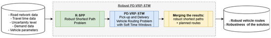
Figure 1. The concept of integrating the Robust Shortest Path Problem (R-SPP) with M-VRP problem.

The road database includes, among other elements, the road-network topology, arc travel times, and the associated level of uncertainty. It also stores the parameters used to normalize the objective function of the $(R-SPP)$ model. The values in $F_i^{SP}$ are determined separately for each study area in which the original vehicle-routing problem is considered. The minimum elements of this set correspond to the shortest path in the network, expressed by time and by distance—i.e., the smallest travel time and the smallest distance found in the matrices ${\widetilde{TT}}^{SP}$ and $D{D}^{SP}$, respectively. The maximum elements of $F_i^{SP}$ correspond to the longest paths in the network, considered separately for time and for distance. At this stage, travel-time uncertainty is represented by the empirical range of variability in the data.

The second database contains the carrier’s information about customers (locations and service characteristics). Additional decision data include the number of vehicles, vehicle capacities, weights of the partial criteria, and the conservatism level. The parameter ${\mathsf{\Gamma }}^{SP}$ is a second lever for setting the uncertainty level and forms part of the carrier’s decision process. Its value may be specified ad hoc by a decision maker (e.g., a transport planner) or by a decision support system. It is also possible to widen the uncertainty set defined in ${\widetilde{TT}}^{SP}$, depending on the decision context. Such a change yields solutions that are more robust to parameter fluctuations.

Because the robust shortest-path module is an integral component of the overall robust routing method, the relationships between criteria in $(R-SPP)$ must mirror those in $(M-VRP)$. The $(R-SPP)$ model accounts for the first two criteria; given the convexity of the aggregation function (1), the weight used in $(R-SPP)$ takes the form: ${\omega }^{SP}={\displaystyle \frac{{\omega }_1}{{\omega }_1+{\omega }_2}}$.

In the robust shortest-path module, computations are performed for every pair of vertices in the set $V_S$. The resulting database contains: (i) the pairwise travel times $TT$, computed with customer service windows and data uncertainty; (ii) the distance matrix $DD$, representing the lengths of the shortest robust paths; and (iii) the set of robust paths $P^{SP}$. The normalization parameters for the partial criteria are also updated here. The sets $F_{N1}^{VRP}$ and $F_{N2}^{VRP}$ are obtained for each database instance and can take the following values:

• $F_1^{min}$: objective value for the modified model $(M-VRP)$, which omits time-window constraints and minimizes only the first sub-criterion $f_1$;
• $F_2^{min}$: objective value for the modified model $(M-VRP)$, which omits time-window constraints and minimizes only the first sub-criterion $f_2$;
• $F_3^{min}=F_4^{min}=0$;
• $F_5^{min}=1$;
• $F_1^{max}$: objective value for the modified model $(M-VRP)$, which omits time-window constraints and maximizes only the first sub-criterion $f_1$;
• $F_2^{max}$: objective value for the modified model $(M-VRP)$, which omits time-window constraints and maximizes only the first sub-criterion $f_1;$
• $F_3^{max}={\sum }_{i\in V{P}_C}(e_i-e_i^{\#})$;
• $F_4^{max}={\sum }_{i\in V{P}_C}(l_i^{\#}-l_i)$;
• $F_5^{max}=K$.

Data from the robust-path module are then passed to the vehicle-routing module. Using $(M-VRP)$, routes are obtained and collected in the set $R^{VRP}$. These routes define the customer visit sequence and the arrival times. To recover the exact geometric trajectories of the routes, the outputs of both modules must be combined.

Decomposition is adopted to place uncertainty where it arises—on road arcs—while keeping the vehicle-routing layer compact and numerically stable. Embedding uncertain travel times directly in VRP time-propagation constraints can inflate the formulation under budgeted sets and offer limited control over the protection–cost trade-off. By contrast, handling uncertainty in a robust shortest-path (R-SPP) preprocessing stage (with the same time–distance criteria used by the VRP) respects how congestion accumulates on arcs and passes inter-customer costs to an otherwise standard M-PD-VRP-STW with soft windows and pickup–delivery precedence. This “data preprocessing” design reduces model stiffness and supports parallel computation of pairwise paths; operationally, it mirrors how dispatch systems compute OD costs before tour construction. The approach aligns with budgeted-uncertainty robust optimisation for networks (tractable linear counterparts with interpretable conservatism $\mathsf{\Gamma }$) and with reliable shortest-path theory, while avoiding over-conservatism and modelling artefacts of direct robust counterparts inside the VRP.

4. Experimental Design and Data: Integrating R-SPP Preprocessing with the Multicriteria PDVRP-STW

The numerical experiments are designed to emulate last-mile freight operations in an urban setting. The underlying road network corresponds to the road network of a real city, and the depot node is interpreted as a logistics terminal from which delivery vehicles depart and to which they return at the end of the planning horizon. Customer nodes are located at points that represent delivery and pickup locations (e.g., shops, depots, or customer facilities) scattered across the urban area. Each customer demand reflects a quantity of goods to be transported, and vehicle capacity is calibrated to typical payloads of light or medium delivery trucks.

The time windows assigned to customers correspond to delivery or collection slots that can arise from store opening hours, access regulations (such as time-restricted delivery zones), or pre-booked service intervals. In this way, the PDVRP-STW instances used in the experiments are consistent with urban freight distribution scenarios, in which vehicles must respect both capacity and timing constraints while operating on a congested road network.

4.1. Robust Shortest-Path (R-SPP) Module and Datasets

R-SPP was exercised on three datasets: (i) a family of randomly generated illustrative networks of increasing size labelled R-100, R-225, R-400, R-625, R-900 and R-1225; (ii) a calibrated Kraków–centre road network with link travel times produced by AIMSUN 24.0 in microscopic traffic simulation (Figure 2); and (iii) a large Kraków agglomeration network where expected times were derived from link length and speed limits and deviations sampled uniformly. The Kraków–centre simulation was calibrated against screenline counts: the model met the stated average fit target, and GEH < 5 for 85.36% of measurements, indicating statistical adequacy for generating inter-customer costs.

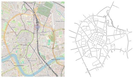
Figure 2. The analysed area of the city of Kraków (left) and its model in the AIMSUN 24.0 software (right).

The first experiment aimed to determine the average optimisation time for a given case as a function of the analysed network’s size. The results are presented in Table 1, which show the computation time for a randomly selected pair of points in the network under study. Values in the table marked with an asterisk indicate that the algorithm did not reach an optimal solution but terminated upon meeting the stopping criterion—a computation time limit of 60 s.

Table 1. Computation time as a function of network size and the conservatism-control parameter.

			Computing Time [Seconds]
Case	No. Node	No. Arcs	ΓSP = 0	ΓSP = 10	ΓSP = 20	ΓSP = 30	ΓSP = 40	ΓSP = 50	ΓSP = 60	ΓSP = 70	ΓSP = 80	Mean
R-100	100	360	0.11	0.12	0.12	0.11	0.11	0.11	0.11	0.11	0.11	0.11
R-220	225	840	0.16	0.39	0.38	0.25	0.23	0.20	0.18	0.18	0.19	0.23
R-400	400	1520	0.35	0.49	1.24	0.69	0.44	0.41	0.61	0.41	0.43	0.53
R-625	625	2400	0.69	1.73	8.92	3.22	1.94	1.43	1.07	0.96	0.90	2.06
R-900	900	3780	1.36	2.85	7.06	12.41	6.33	12.16	2.71	2.54	2.07	4.86
R-1225	1225	4760	2.34	5.83	60.90 *	60.97 *	60.94 *	21.57	60.95 *	12.67	9.10	27.71
Kraków-centre	250	546	0.18	0.18	0.18	0.18	0.19	0.17	0.18	0.18	0.17	0.18
Kraków	2101	5094	8.73	12.06	11.95	11.82	13.81	13.04	13.62	14.14	11.01	12.17

A characteristic feature of NP-hard problems is the exponential growth of computation time with respect to graph size. Another property of such models is the existence of a threshold point, beyond which the optimisation time increases sharply and becomes impractical. In the analysed case, the practical applicability of the model $(R-SPP)$ to subsequent VRP-related analyses can be identified at around 500 network nodes. For this network size, the optimisation time remains below one second. Such computational speed is crucial, given that the model is used to calculate the shortest paths between all pairs of customers in the system.

4.2. Positive and Negative Aspects of Applying the $(R-SPP)$ Model

The final analysis evaluates the benefits and drawbacks of accounting for uncertainty when computing urban paths. The study was carried out on the real road network of central Kraków; traffic data were obtained as in the previous experiments. For 20 randomly selected vertices, all ordered origin–destination pairs were considered, yielding 380 cases. The $(R-SPP)$ model was run with two conservatism settings: ${\mathsf{\Gamma }}^{SP}=0$ (deterministic version) and ${\mathsf{\Gamma }}^{SP}=10$ (robust version). The uncertainty set was defined as the interval between the daily mean travel time and the maximum observed during 15:00–18:00 (the afternoon peak in Kraków). The deterministic version served as the baseline (parameters equal to daily mean times). The objective weight was set to ${\omega }^{SP}=0.75$ (the justification for this choice is provided in Appendix A). For both versions, changes in path length (distance) were also recorded.

Given the dynamic nature of urban traffic, two comparison variants were examined:

• Variant 1. Cost of the deterministic and robust paths under the assumed deviations (a fully accurate forecast).
• Variant 2. Costs when realized deviations differ from the assumptions. Differences were generated by multiplying the deviation from the mean by a factor in $[0.5, 1.5]$ (a partially inaccurate forecast).

Reduction relative to the deterministic version was computed as: $\mathrm{R}\mathrm{E}\mathrm{D}={\displaystyle \frac{F_{\mathrm{D}\mathrm{E}\mathrm{T}}-F_{\mathrm{R}\mathrm{O}\mathrm{B}}}{F_{\mathrm{D}\mathrm{E}\mathrm{T}}}}\times 100\%,$ where $F_{\mathrm{D}\mathrm{E}\mathrm{T}}$ and $F_{\mathrm{R}\mathrm{O}\mathrm{B}}$ denote the cost of the deterministic and robust paths (time or distance). Negative RED indicates an increase in cost under the robust solution. Results are shown in Table 2.

Table 2. Positive and negative aspects of applying the $(R-SPP)$ model relative to the deterministic SPP with respect to travel time and path length.

Reduction [%]	Travel-Time								Distance
	Variant 1				Variant 2
	Count	Min.	Mean	Max.	Count	Min.	Mean	Max.	Count	Min.	Mean	Max.
Positive	66	0.77	9.40	37.31	57	0.00	11.98	54.35	21	0.78	1.95	5.03
Negative	6	−5.08	−4.39	−3.92	16	−20.13	−8.04	−0.14	51	−18.89	−6.55	−0.63
Neutral	308	0.00	0.00	0.00	307	0.00	0.00	0.00	308	0.00	0.00	0.00
	Mean	8.25			Mean	7.59			Mean	−4.07

Incorporating travel-time uncertainty in path planning can deliver material time savings. Although most cases remain unchanged, nearly one in five deterministic paths is outperformed by the robust alternative. In Variant 1, the average time reduction is 8.25%, with a maximum of 37.31%; deteriorations are rare (6 cases) and modest (up to ~5%). In Variant 2, potential time gains increase with larger mis-specification of deviations (mean 7.59%, maximum 54.35%). Time gains are often achieved at the expense of distance: on average, about one in three paths with positive time reduction shows negative distance reduction. Overall, the time benefits outweigh the average distance costs, which is particularly relevant for operators prioritizing service punctuality. Accounting for uncertainty at the path/routing stage can improve arrival-time accuracy and service quality.

Because robust shortest paths feed the vehicle-routing problem, potential gains at the VRP level are expected to be at least comparable; this hypothesis is examined empirically in the subsequent part of the study.

4.3. Deterministic Baseline Versus Integrated Robust Approach in VRP

The following description synthesizes the methodology for integrating the robust shortest path problem (R-SPP) with a single routing model (M-VRP) for the deterministic and robust variants in the context of VRP-STW. In the deterministic variant, inter-node costs (time and distance) are obtained by computing deterministic shortest paths with R-SPP at a conservatism level ${\mathsf{\Gamma }}^{SP}=0$, that is, using mean arc travel times. The resulting time and distance matrices serve as input to the (M-VRP) model, which remains unchanged in structure, number of sub-criteria, normalization scheme, and all other assumptions (soft time windows, capacities, fleet size, and demand–supply data).

In the robust variant, travel-time uncertainty is modeled at the (R-SPP) layer via an uncertainty set defined from the mean and standard deviation for each network arc and for each hour of the day (one-hour time slices derived from traffic data or simulation). The protection level is governed by the parameter ${\mathsf{\Gamma }}^{SP}$ (e.g., low, medium, and maximum settings), which yields shortest robust paths for all customer–depot pairs. These paths produce time and distance matrices that are then used in the same (M-VRP) model. This decomposition supplies (M-VRP) with OD costs that already account for risk, while the routing model’s logic and settings remain identical to those in the deterministic case.

Experiments are conducted on a reference set of instances comprising randomly generated customer sets with urban parcel-distribution characteristics, a specified structure of soft time windows, a depot operating from 06:00 to 21:00, and up to five vehicles with 1000 kg capacity. The deterministic variant uses this same set, whereas the robust variant replicates the instances for different ${\mathsf{\Gamma }}^{SP}$ levels. Comparability is ensured by an identical computational pipeline and identical (M-VRP) parameters; the only difference between variants lies in how OD costs are obtained (mean times versus robust times).

Solution quality is evaluated using total travel time and total distance, punctuality measures (aggregate earliness and lateness and their counts), the number of routes, and computation times: the (M-VRP) solve time and the total time (R-SPP + M-VRP). For selected metrics, reduction relative to the deterministic variant is reported as $\mathrm{R}\mathrm{E}\mathrm{D}={\displaystyle \frac{F_{\mathrm{D}\mathrm{E}\mathrm{T}}-F_{\mathrm{R}\mathrm{O}\mathrm{B}}}{F_{\mathrm{D}\mathrm{E}\mathrm{T}}}}\cdot 100\%$, enabling an unambiguous interpretation of the gains or costs associated with introducing robustness at the path-computation stage while keeping the routing model’s objectives and logic unchanged.

Urban traffic is highly variable, so evaluating solutions solely on input data can be misleading because realized conditions may differ from assumptions. To assess the deterministic (DET) and robust (ROB) variants, six random scenarios were generated. In each scenario $r$, for every arc $(i,j)$, the travel time was set to the mean plus a perturbation proportional to the standard deviation and a uniform factor ${\epsilon }_r$; ${\epsilon }_r$ controls the magnitude of deviations. The ranges corresponded to 20%, 50%, 80%, 100%, 120%, and 150% levels. The first two scenarios represent under-realization of variability (milder-than-expected conditions), the next two approximate the planning assumptions, and the last two exceed the forecast (e.g., incidents). For each scenario, 50 independent realizations were created; on each, the quality of the finalized M-VRP routes (built from DET or ROB OD costs) was evaluated using total travel time and distance, punctuality measures (earliness/lateness and their counts), the number of routes, and computation times. Results were compared as ROB minus DET, reporting the mean, minimum, and maximum over the 50 runs. This procedure mirrors how plans are validated when actual traffic partly or fully departs from the data used for planning. The comparison was performed by computing (i) the differences in evaluation-parameter values between the variants and (ii) the reduction (percentage, RED) of selected evaluation parameters.

The study assessed how the conservatism level ${\mathsf{\Gamma }}^{SP}$ in the R-SPP layer affects differences between deterministic (DET) and robust (ROB) routing outcomes, considering the number of customers and the realized degree of uncertainty. In most cases time savings outweighed losses: over 82% of instances favored ROB, with an average gain of 10.7 min (range 0.1–38.8 min). The largest count of losses occurred under very high conservatism (maximum ${\mathsf{\Gamma }}^{SP}$; worst-case oriented), with nearly 68% of cases showing an average loss of 3.8 min, while the maximum loss did not exceed 10.1 min for any ${\mathsf{\Gamma }}^{SP}$ level. As the gap between assumed and realized travel times increases, potential gains rise and losses decrease; there was no clear correlation with the number of customers. Low conservatism reduces both risk and the magnitude of attainable gains. Notably, even in scenarios exceeding the assumed uncertainty bounds (e.g., 120% and 150%), ROB solutions remain on average superior to DET. In the tested set, the best trade-off was observed for ${\mathsf{\Gamma }}^{SP}=20$; selecting ${\mathsf{\Gamma }}^{SP}$ should depend on the uncertainty profile, network structure, and forecast quality, and can be supported by rule-based decision support systems.

Figure 3 reports the travel-time reduction relative to the deterministic solution. The maximum gain exceeds 14%, while the largest loss is about 7%. On average, across all tested variants and demand configurations, the reduction in travel time is slightly above 3%, and the distribution of outcomes is clearly skewed towards improvements rather than deteriorations. This asymmetry indicates that the robust plans successfully exploit a substantial portion of the potential gains associated with accounting for travel-time variability, while keeping adverse effects within a relatively narrow band.

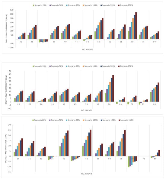
Figure 3. Mean travel-time difference (DET − ROB) as a function of the number of customers and the realized uncertainty level. (Top) plot: ${\mathsf{\Gamma }}^{SP}=5$ (“Gamma 5”); (middle) plot: ${\mathsf{\Gamma }}^{SP}=20$ (“Gamma 20”); (bottom) plot: ${\mathsf{\Gamma }}^{SP}={\mathsf{\Gamma }}_{\mathrm{m}\mathrm{a}\mathrm{x}}$ (“Gamma max”).

A further pattern visible in Figure 3 is that the percentage reduction tends to decline as the number of customers increases. This suggests that the absolute time advantage of the robust solution remains of similar magnitude across instance sizes, but becomes proportionally smaller as the baseline (deterministic) total travel time grows with the number of stops. Importantly, the absence of a clear positive correlation between instance size and relative losses supports the view that the robust approach does not become systematically more conservative or inefficient for larger problems; rather, it offers a bounded trade-off between additional planned time and improved protection against delays.

Optimisation based on the worst-case changes yields unsatisfactory results. The average potential gain in travel time across all scenarios is negligible, only 1.3 min. Of course, there are scenarios in which these gains are high, but they are simultaneously accompanied by the risk of losses. Assuming the worst possible range of travel-time variation (maximum Gamma) makes the resulting solution overly pessimistic when evaluated under actual conditions. This is yet another confirmation of a well-known property of such approaches, repeatedly noted in the robust optimisation literature. Using large values of the conservatism parameter may be justified in situations where large fluctuations in travel time on particular links are expected, where unusual incidents occur in the road network (temporary closures, roadworks, temporary traffic management, etc.), or where the travel-time forecast is suspected to have a large estimation error. This is confirmed by the decreasing loss observed, for example, for instances with 35, 45 or 80 customers across successive random scenarios. This indicates that the larger the discrepancy between the value assumed in the model and the realised travel time, the more the potential gains increase and the losses decrease.

Adopting a low level of solution conservatism reduces the above effects, but at the same time also reduces the potential gains in travel time. A characteristic feature of robust optimisation is that it aims to ensure solution stability even when the model parameters exceed the bounds of the assumed uncertainty set. This is particularly visible in the 120% and 150% scenarios, where some arcs in the random data set are assigned values higher than those specified in the model’s uncertainty set. The solution obtained, which is robust to fluctuations, remains more favourable than the deterministic solution. Moreover, it can be observed that an increase in the number of customers is not correlated with the potential gains or losses in travel time.

For distance, Table 3 shows the difference in route length (ROB vs. DET) and the percentage increase/decrease relative to the deterministic solution. Results indicate that time savings under variable traffic conditions are often achieved at the expense of distance: in most cases ROB routes are longer, yet the mean increase is only ~2.3%, and in ~30% of cases the total distance decreases. No clear correlation was observed between distance changes and either the number of customers or the conservatism level.

Table 3. Difference in distance between the deterministic and robust variants as a function of the number of customers and the conservatism parameter, along with the percentage increase/decrease.

Distance Difference [Meters]
Gamma	No. Clients
	20	25	30	35	40	45	50	55	60	65	70	75	80
5	−1275	488	−1271	1106	−110	−146	−1056	1964	−1469	−1639	−634	448	−2481
20	1032	253	708	135	−1059	1264	−1689	−858	5007	−3719	−6885	−3206	−209
max	583	−419	−1523	−2714	−1555	−4282	2900	−2799	405	−1219	−8706	-	−4325
Mean	114	108	−696	−492	−908	−1055	52	−565	1315	−2192	−5408	−1380	−2338
Percentage Increase/Decrease [%]
5	−1.7	1.6	−0.6	2.7	−2.3	−2.1	2.0	1.1	−0.8	−0.7	−0.2	2.1	−4.5
20	2.7	0.8	−2.0	−1.1	−1.5	1.5	−2.3	−2.2	5.7	−5.4	−8.8	−5.1	0.7
max	0.0	−1.6	−2.7	−4.7	−0.9	−4.6	0.5	−1.4	0.3	−2.3	−11.1	-	−3.7
mean	0.33	0.27	−1.77	−1.03	−1.57	−1.73	0.07	−0.83	1.73	−2.80	−6.70	−1.50	−2.50

In the simulation of random scenarios and the subsequent evaluation, earliness does not imply driver waiting: service starts immediately with an additional penalty cost, consistent with soft time windows assumed in the VRP model. Likewise, tardiness does not imply a failed delivery—the route continues and the execution cost increases. In addition to the total earliness and tardiness times, the counts of early/late services were computed for each solution. Results are presented in Table 4 for earliness and for the counts of early services. Negative values mean that robust solution increased the KPI.

Table 4. Mean result for earliness and for the counts of early services.

Scenario	KPI	No. Clients
		20	25	30	35	40	45	50	55	60	65	70	75	80
Gamma 5	Mean waiting time [min]	8.2	7.7	7.2	8.0	8.3	10.9	11.3	10.5	9.8	11.0	13.0	10.9	13.0
	Mean counts of early services	−1.8	−2.0	−1.9	−2.4	−2.5	−3.4	−4.2	−3.7	−3.6	−4.5	−0.3	−5.0	−5.8
Gamma 20	Mean waiting time [min]	10.8	7.1	7.0	10.4	9.7	12.3	13.5	10.7	9.1	10.7	10.4	14.3	14.9
	Mean counts of early services	−2.1	−2.5	−2.3	−3.1	−3.3	−3.8	−4.8	−5.3	−5.2	−5.3	−4.1	−6.1	−6.4
Gamma max	Mean waiting time [min]	9.3	8.4	2.3	9.4	9.4	14.4	13.2	10.1	9.9	24.3	14.5	-	32.1
	Mean counts of early services	−2.0	−2.5	0.0	−2.9	−3.2	−3.9	−4.8	−5.3	−5.2	−6.5	−5.5	-	−6.6

Solving the VRP under these assumptions yields the customer visit sequence, the assignment of customers to routes, and the schedule of arrivals. If the search for a solution accounts for travel-time variability, it affects the planned arrival times at customers. In almost all cases—regardless of the number of customers and the conservatism level—the average earliness time is higher than in the deterministic solution. The magnitude of the difference is strongly driven by the realized uncertainty level. When the forecast is overly pessimistic or the uncertainty set is too wide (20%, 50%, and 80% scenarios), the robust approach exhibits substantially larger earliness than the deterministic one. Conversely, when the expected values and standard deviations are well calibrated (100% and 120% scenarios), the differences are markedly smaller. The average earliness difference per customer: 2.1 min for ${\mathsf{\Gamma }}^{SP}=5$, 2.5 min for ${\mathsf{\Gamma }}^{SP}=20$, and 9.2 min for ${\mathsf{\Gamma }}^{SP}=\mid VP\mid +\mid C\mid$. For the first two ${\mathsf{\Gamma }}^{SP}$ levels, per-customer differences are small enough to be barely noticeable in real distribution operations. It was also confirmed that an extreme worst-case configuration (maximum ${\mathsf{\Gamma }}^{SP}$) is inadequate for VRP: both the earliness time and the number of early services are, on average, the largest. Results are presented in Table 5 for tardiness and for the counts of late services.

Table 5. Mean result for tardiness and for the counts of late services.

Scenario	KPI	No. Clients
		20	25	30	35	40	45	50	55	60	65	70	75	80
Gamma 5	Mean tardiness time [min]	19.4	28.2	15.5	24.0	25.0	27.2	29.8	22.2	22.3	29.6	108.0	26.2	32.8
	Mean counts of late services	1.3	1.5	1.4	3.9	3.8	3.7	6.5	6.6	5.1	8.4	0.5	9.2	11.2
Gamma 20	Mean tardiness time [min]	21.2	21.2	14.3	22.7	24.9	24.1	30.8	22.4	23.7	27.9	24.3	26.8	30.6
	Mean counts of late services	1.6	2.1	2.2	3.7	4.4	4.5	7.5	6.2	5.6	9.2	7.3	11.2	13.6
Gamma max	Mean tardiness time [min]	19.4	24.0	15.2	23.3	22.4	24.5	27.9	23.9	22.4	27.0	19.7	-	28.2
	Mean counts of late services	1.5	1.8	0.6	3.9	4.2	4.6	6.3	6.6	6.0	8.5	7.0	-	13.3

Tardiness provides an additional quality metric. Across the variants, this metric is consistently in favor of the robust approach: the difference relative to the deterministic solution is positive in all analyzed cases, indicating the advantage of ROB. Importantly, this improvement is not merely a compensation for increased earliness—the values are several times larger. For example, the average tardiness reduction per customer for the 100% and 120% scenarios amounted to 12.7 min (${\mathsf{\Gamma }}^{SP}=5$), 12.3 min (${\mathsf{\Gamma }}^{SP}=20$), and 10.4 min (${\mathsf{\Gamma }}^{SP}=\mid VP\mid +\mid C\mid$). In addition, a relationship between the potential gains and the number of customers was observed, with an average $R^2$ exceeding 76%.

5. Results, Discussion, and Environmental Implications

This section compares a deterministic variant with a robust variant that integrates a robust shortest-path preprocessing stage with a single, normalized multicriteria urban routing model with soft time windows. The routing formulation, objective normalization, constraints, and solver settings are identical in both variants; the only difference lies in how origin–destination (OD) costs are obtained. The deterministic baseline uses shortest paths computed from mean arc travel times, whereas the robust variant uses shortest paths computed under budgeted uncertainty with a tunable conservatism parameter Γ. Reported indicators include total travel time, total distance, lateness/earliness and their counts, the number of routes, and computation times. These are standard operational outputs and can also serve as inputs to subsequent energy or environmental assessments where activity-based methods are employed.

The main operational results can be summarised as follows. Late arrivals are consistently lower in the robust variant across all tested settings. In scenarios that match the planning assumptions, the average reduction in lateness per customer is on the order of ten minutes or more, depending on the conservatism level. Total travel time also tends to improve: the average reduction across all cases is above three percent, with the best cases exceeding fourteen percent and the worst cases showing losses of about seven percent. These time benefits do not come from adding routes; the number of routes remains comparable, and the time needed to solve the routing model is similar once the cost matrices are available. The main price of robustness is small: total distance increases by about two to three percent on average, although roughly one third of the instances show shorter distances because of more effective routing. Early arrivals increase slightly—typically by a few minutes per customer at moderate conservatism—and can rise more under very high conservatism. A moderate conservatism level gives the best balance between protection and cost; extremely high protection leads to unnecessary pessimism, while very low protection limits potential gains in punctuality. The dependence on problem size is limited: total travel time shows no clear link to the number of customers, whereas improvements in lateness tend to be larger for bigger instances, which offer more opportunities to exploit robustness. Taken together, these reliability improvements and time effects provide a transparent operational profile—time, distance, and schedule-adherence metrics—that is directly compatible with environmental performance analyses without altering the routing formulation.

For practice, the robust variant constitutes a safer planning policy when punctuality and service-level compliance are priorities. Because OD costs are computed up front and uncertainty is concentrated in the path layer, the computational overhead is localized in a module that scales well and can be parallelized, while the routing solver remains unchanged. Although the present study does not explicitly quantify energy use or emissions, the observed operational outcomes—improved schedule adherence and generally shorter total travel time with only small, predictable adjustments in distance— can be expected to be consistent with lower delay propagation, fewer unproductive stops/idling, and more stable tour execution. These effects would, in many standard activity-based frameworks, reduce the activity drivers that typically underpin energy and emission inventories in urban deliveries (time-in-traffic, stop–go events, detours) without altering the routing formulation. Because uncertainty handling is concentrated in the path layer and the same routing model is used across variants, the reported operational indicators (total travel time, distance, lateness/earliness and their counts, number of routes, and computation times) are readily mappable into standard activity-based energy or environmental assessments. In practice, the conservatism parameter Γ provides a transparent policy lever for planners to balance protection and cost in line with service-level objectives, while exposing the operational metrics needed for downstream environmental appraisal.

Further work should focus on adaptive, data-driven selection of the conservatism parameter (possibly different by arc, zone, or time of day), explicit risk-aware objective terms in the routing model that make the protection–cost trade-off explicit, finer time discretization and better modelling of congestion along paths, dynamic re-optimization in a rolling-horizon setting with real-time data, calibration of penalty weights and normalization from historical performance, uncertainty sets that are robust to distributional errors, validation on multiple cities and larger networks, and extensions that account for additional costs and constraints such as energy use, emissions, depot time windows, and driver rules. These steps can generalize the observed benefits, align protection with operational realities, and further reduce timing risk without materially increasing distance.

In summary, this study compared a deterministic and a robust uncertainty treatment for urban pickup-and-delivery routing with soft time windows on a real road network, keeping the routing formulation, normalization, and solver settings fixed. Modelling uncertainty on the road graph and then solving a single, normalised multicriteria M-PD-VRP-STW produced clear operational benefits. Relative to deterministic preprocessing, robust shortest paths delivered shorter travel times and fewer late services without inflating the number of tours, with only a modest change in distance—improvements that speak directly to reliability and service quality in city logistics. The integration of robust path preprocessing with standard urban routing thus yields reliability gains within an OD-first pipeline and delivers operational outputs directly usable at the environment interface.

References

- Bent, R.; Van Hentenryck, P. A two-stage hybrid local search for the vehicle routing problem with time windows. Transp. Sci. 2004, 38, 515–530. [Google Scholar] [CrossRef]
- Osman, I.H.; Wassan, N.A. A reactive tabu search meta-heuristic for the vehicle routing problem with back-hauls. J. Sched. 2002, 5, 263–285. [Google Scholar] [CrossRef]
- Pisinger, D.; Ropke, S. A general heuristic for vehicle routing problems. Comput. Oper. Res. 2007, 34, 2403–2435. [Google Scholar] [CrossRef]
- Ropke, S.; Pisinger, D. An adaptive large neighborhood search heuristic for the pickup and delivery problem with time windows. Transp. Sci. 2006, 40, 455–472. [Google Scholar] [CrossRef]
- Russell, R.A.; Chiang, W.C. Scatter search for the vehicle routing problem with time windows. Eur. J. Oper. Res. 2005, 169, 606–622. [Google Scholar] [CrossRef]
- Taillard, E.D. A heuristic column generation method for the heterogeneous fleet VRP. RAIRO-Oper. Res. 1999, 33, 1–14. [Google Scholar] [CrossRef]
- Tan, K.C.; Cheong, C.Y.; Goh, C.K. Solving multiobjective vehicle routing problem with stochastic demand via evolutionary computation. Eur. J. Oper. Res. 2007, 177, 813–839. [Google Scholar] [CrossRef]
- Tarantilis, C.D.; Kiranoudis, C.T.; Vassiliadis, V.S. A threshold accepting metaheuristic for the heterogeneous fixed fleet vehicle routing problem. Eur. J. Oper. Res. 2004, 152, 148–158. [Google Scholar] [CrossRef]
- Russo, F.; Comi, A. Urban Courier Delivery in a Smart City: The User Learning Process of Travel Costs Enhanced by Emerging Technologies. Sustainability 2023, 15, 16253. [Google Scholar] [CrossRef]
- Bianchi, L.; Dorigo, M.; Gambardella, L.M.; Gutjahr, W.J. A survey on metaheuristics for stochastic combinatorial optimization. Nat. Comput. 2009, 8, 239–287. [Google Scholar] [CrossRef]
- Fleury, G.; Lacomme, P.; Prins, C. Evolutionary Algorithms for Stochastic Arc Routing Problems. In Applications of Evolutionary Computing; LNCS 3005; Springer: Berlin/Heidelberg, Germany, 2004; pp. 501–512. [Google Scholar]
- Shapiro, A.; Dentcheva, S.; Ruszczyński, A. Lectures on Stochastic Programming: Modeling and Theory; SIAM: Philadelphia, PA, USA, 2009. [Google Scholar]
- Gómez-Marín, C.G.; Comi, A.; Serna-Urán, C.A.; Zapata-Cortés, J.A. Fostering Collaboration and Coordination in Urban Delivery: A Multi-Agent Microsimulation Model. Res. Transp. Econ. 2024, 103, 101402. [Google Scholar] [CrossRef]
- Sungur, I.; Ordonez, F.; Dessouky, M. A robust optimization approach for the capacitated vehicle routing. IIE Trans. 2008, 40, 509–523. [Google Scholar] [CrossRef]
- Solomon, M.M. Algorithms for the vehicle routing and scheduling problems with time window constraints. Oper. Res. 1987, 35, 254–265. [Google Scholar] [CrossRef]
- Han, J.; Lee, C.; Park, S. A robust scenario approach for the vehicle routing problem with uncertain travel times. Transp. Sci. 2014, 48, 373–390. [Google Scholar] [CrossRef]
- Agra, A.; Christiansen, M.; Figueiredo, R.; Hvattum, L.M.; Poss, M.; Requejo, C. The robust vehicle routing problem with time windows. Comput. Oper. Res. 2013, 40, 856–866. [Google Scholar] [CrossRef]
- Solyalı, O.; Cordeau, J.F.; Laporte, G. Robust inventory routing under demand uncertainty. Transp. Sci. 2011, 46, 327–340. [Google Scholar] [CrossRef]
- Ben-Tal, A.; El Ghaoui, L.; Nemirovski, A. Robust Optimization; Princeton University Press: Princeton, NJ, USA, 2009. [Google Scholar]
- Tajik, N.; Tavakkoli-Moghaddam, R.; Vahdani, B.; Mousavi, S.M. A robust optimization approach for pollution routing problem with pickup and delivery under uncertainty. J. Manuf. Syst. 2014, 33, 277–286. [Google Scholar] [CrossRef]
- Folsom, L.; Park, H.; Pandey, V. Dynamic Routing of Heterogeneous Users After Traffic Disruptions Under a Mixed Information Framework. Front. Future Transp. 2022, 3, 851069. [Google Scholar] [CrossRef]
- Donati, A.V.; Montemanni, R.; Casagrande, N.; Rizzoli, A.E.; Gambardella, L.M. Time dependent vehicle routing problem with a multi ant colony system. Eur. J. Oper. Res. 2008, 185, 1174–1191. [Google Scholar] [CrossRef]
- Montemanni, R.; Gambardella, L.M.; Donati, A.V. A branch and bound algorithm for the robust shortest path problem with interval data. Oper. Res. Lett. 2004, 32, 225–232. [Google Scholar] [CrossRef]
- Hoogeboom, M.; Adulyasak, Y.; Dullaert, W.; Jaillet, P. The robust vehicle routing problem with time window assignments. Transp. Sci. 2021, 55, 395–413. [Google Scholar] [CrossRef]
- Metz, L.; Mutzel, P.; Niemann, T.; Schürmann, L.; Stiller, S.; Tillmann, A.M. Delay-resistant robust vehicle routing with heterogeneous time windows. Comput. Oper. Res. 2024, 164, 106553. [Google Scholar] [CrossRef]
- Ghosal, S.; Wiesemann, W. The distributionally robust chance-constrained vehicle routing problem. Oper. Res. 2020, 68, 716–732. [Google Scholar] [CrossRef]
- Ghosal, S.; Ho, C.P.; Wiesemann, W. A unifying framework for the capacitated VRP under risk and ambiguity. Oper. Res. 2023, 72, 425–443. [Google Scholar] [CrossRef]
- Wang, W.; Yang, K.; Yang, L.; Gao, Z. Distributionally robust chance-constrained programming for emergency resource allocation and VRP. Eur. J. Oper. Res. 2023, 120, s0305048323000798. [Google Scholar]
- Vincent, F.Y.; Pham, T.A.; Roberto, B. A robust optimization approach for the VRP with cross-docking under demand uncertainty. Transp. Res. Part E Logist. Transp. Rev. 2023, 173, 103106. [Google Scholar]
- Wang, X.; Zhao, J. Distributionally robust optimization of the VRP with uncertain customers. J. Ind. Manag. Optim. 2025, 21, 1983–2006. [Google Scholar] [CrossRef]
- Adamo, T.; Gendreau, M.; Ghiani, G.; Guerriero, E. A review of recent advances in time-dependent vehicle routing. Eur. J. Oper. Res. 2024, 319, 1–15. [Google Scholar] [CrossRef]
- Filippi, C.; Maggioni, F.; Speranza, M.G. Robust and distributionally robust shortest path problems. Comput. Oper. Res. 2025, 182, 107096. [Google Scholar] [CrossRef]
- Guo, J.; Liu, T.; Song, G.; Guo, B. Solving the robust shortest path problem with multimodal transportation networks. Mathematics 2024, 12, 2978. [Google Scholar] [CrossRef]
- Tang, L.; Luo, R.; Zhou, Z.; Colombo, N. Enhanced route planning with calibrated uncertainty set. arXiv 2025, arXiv:2503.10088. [Google Scholar] [CrossRef]
- Zhang, J. Data-Driven Robust Optimization of the Vehicle Routing Problem. Complexity 2022, 2022, 9064669. [Google Scholar] [CrossRef]
- Soyster, A.L. Convex programming with set-inclusive constraints and applications to inexact linear programming. Oper. Res. 1973, 21, 1154–1157. [Google Scholar] [CrossRef]
- Bertsimas, D.; Sim, M. Robust discrete optimization and network flows. Math. Program. 2003, 98, 49–71. [Google Scholar] [CrossRef]
Disclaimer/Publisher’s Note: The statements, opinions and data contained in all publications are solely those of the individual author(s) and contributor(s) and not of MDPI and/or the editor(s). MDPI and/or the editor(s) disclaim responsibility for any injury to people or property resulting from any ideas, methods, instructions or products referred to in the content. |
© 2025 by the author. Licensee MDPI, Basel, Switzerland. This article is an open access article distributed under the terms and conditions of the Creative Commons Attribution (CC BY) license (https://creativecommons.org/licenses/by/4.0/).