A Hybrid AI-Stochastic Framework for Predicting Dynamic Labor Productivity in Sustainable Repetitive Construction Activities

Abstract

Accurate real-time prediction of labor productivity is crucial for the successful management of construction projects. However, it remains a significant challenge due to the dynamic and uncertain nature of construction environments. Existing models, while valuable for planning and post-analysis, often rely on historical data and static assumptions, rendering them inadequate for providing actionable, real-time insights during construction. This study addresses this gap by suggesting a novel hybrid AI-stochastic framework that integrates a Long Short-Term Memory (LSTM) network with Markov Chain modeling for dynamic productivity forecasting in repetitive construction activities. The LSTM component captures complex, long-term temporal dependencies in productivity data, while the Markov Chain models probabilistic state transitions (Low, Medium, High productivity) to account for inherent volatility and uncertainty. A key innovation is the use of a Bayesian-adjusted Transition Probability Matrix (TPM) to mitigate the “cold start” problem in new projects with limited initial data. The framework was rigorously validated across four distinct case studies, demonstrating robust performance with Mean Absolute Percentage Error (MAPE) values predominantly in the “Good” range (10–20%) for both the training and test datasets. A comprehensive sensitivity analysis further revealed the model’s stability under data perturbations, though performance varied with project characteristics. By enabling more efficient resource utilization and reducing project delays, the proposed framework contributes directly to sustainable construction practices. The model’s ability to provide accurate real-time predictions helps minimize material waste, reduce unnecessary labor costs, optimize equipment usage, and decrease the overall environmental impact of construction projects.

1. Introduction

Labor productivity is a crucial aspect in the successful delivery of projects within the construction industry, directly impacting project schedules, cost adherence, and overall profitability. Beyond economic considerations, labor productivity plays a pivotal role in advancing construction sustainability. Higher productivity reduces material waste through better planning, minimizes energy consumption by shortening project durations, optimizes resource allocation to prevent overuse, and decreases the carbon footprint associated with extended construction activities. The construction sector accounts for approximately 39% of global carbon emissions and consumes significant natural resources, making productivity improvements a critical pathway toward sustainable development [1]. Its critical role is highlighted by the substantial portion of project expenses attributed to labor. Industry data consistently shows that labor costs typically account for 20% to 40% of total construction project costs [2,3]. Such high labor costs amplify the consequences of productivity decline, which has persisted over recent decades. For instance, U.S. construction labor productivity diminished by over 30% between 1970 and [4]. This stagnation has been persistent, with the U.S. experiencing negative productivity growth in construction between 2000 and 2021 [5], underscoring a critical issue that requires advanced forecasting and management strategies.

Several studies explored various methodologies to predict labor productivity in the construction industry. Early methods often relied on learning curve models, which measure productivity improvements in repetitive tasks [6]. While foundational for insight into long-term trends, these models frequently assume predictable learning patterns and struggle to account for dynamic, real-time disruptions. The emergence of Artificial Neural Networks (ANNs) marked a significant advancement, enabling the handling of complex, nonlinear relationships in productivity forecasting by integrating historical data and expert judgment [7,8]. However, ANNs typically rely on broad historical datasets that may not fully capture the evolving conditions on an active construction site. Time-series analysis has also been employed to identify temporal patterns and forecast productivity, providing insights into historical trends [9,10]. Yet, these models often struggle to adapt in real time to sudden, unforeseen changes. More recently, System Dynamics (SD) and Agent-Based Modeling (ABM) provided frameworks for simulating complex interactions and emergent behaviors, proving decisive for understanding systems and exploring ‘what-if’ scenarios [11].

Despite these efforts, a critical research gap persists in accurately and reliably predicting labor productivity in real time during the construction stage. Existing models, while valuable for planning and post-analysis, often fall short of providing actionable insights for immediate decision-making on dynamic construction sites. This limitation stems from their reliance on historical data and static assumptions, which fail to adapt to the continuous, unpredictable changes inherent in construction environments, such as unforeseen site conditions, material delays, equipment breakdowns, or shifts in crew composition. Furthermore, current methods frequently provide macro-level or delayed productivity assessments, which are insufficient for identifying and mitigating productivity losses as they occur. This study addresses this gap by offering a novel hybrid framework that integrates advanced analytical techniques to provide dynamic, real-time productivity predictions. The implications of this study are significant. It will empower project managers with fine-grained, instantaneous feedback, enabling proactive identification and mitigation of productivity deviations. It is expected to lead to enhanced project performance, reduced cost and schedule overruns, and improved overall efficiency in the delivery of construction projects.

The remainder of this manuscript is structured as follows: Section 2 displays a comprehensive review of the existing literature on labor productivity forecasting models, including an in-depth analysis of studies that integrate Markov Chains with Long Short-Term Memory (LSTM) networks, and further delineates the identified research gaps. Section 3 describes the proposed methodology, including data acquisition, preprocessing, development of the hybrid LSTM model, and integration with Markov Chain modeling. Section 4 presents the results and provides a thorough discussion of the findings. Finally, Section 5 concludes the study, summarizes its contributions, and outlines avenues for future research.

2. Literature Review

2.1. Review of the Labor Productivity Forecasted Model

Accurate labor productivity forecasting is crucial for effective construction project management, as it impacts scheduling, resource allocation, and cost control. Despite several models, a significant gap remains in predicting real-time productivity during the construction implementation. This section reviews existing models, highlighting their contributions and limitations, emphasizing the need for further research into dynamic, in situ productivity forecasting.

Learning curve models had historically been fundamental for predicting productivity improvements in repetitive tasks. For instance, Rahal and Khoury [12] utilized a fuzzy-based system to determine learning ranges and reduce congestion in linear activities. Similarly, Khanh et al. [6] applied the straight-line model to high-rise building projects, showing productivity gains over repetitive floors. While useful for initial planning and perception of long-term trends, these models often assume predictable learning patterns and struggle to account for dynamic, real-time disruptions and unforeseen factors during project execution.

ANNs represent a significant advancement in handling complex, nonlinear relationships in productivity forecasting. Portas and Abourizk [7] pioneered the use of ANNs for concrete formwork, integrating historical data with expert judgment to improve estimation accuracy. Heravi et al. [8] further demonstrated the capability of ANNs to forecast labor productivity in power plant construction, highlighting their ability to quantify the complex mapping of multiple influencing factors. However, ANNs typically rely on historical datasets for training, which may not fully capture the real-time, changing conditions of an active construction site, thereby reducing predictive accuracy across different scenarios.

Time-series analysis provides a data-driven approach to predict by identifying temporal patterns. Kim et al. [9] developed a time-series model to forecast the productivity of newly added workers, integrating site-learning effects. Jacobsen et al. [10] studied probabilistic time-series forecasting, providing distributions of future productivity metrics rather than single-point estimates. While these models excel at leveraging historical trends, their effectiveness in real-time adaptation to sudden, unforeseen changes on a live construction site remains a challenge. The dynamic nature of construction, with its inherent variability in site conditions, resource availability, and unforeseen events, often leads to deviations that are difficult for purely historical time-series models to predict with high accuracy in real time.

System Dynamics (SD) and Agent-Based Modeling (ABM) give frameworks for simulating complex interactions and emergent behaviors. Nasirzadeh and Nojedehi [11] used SD to model interrelated factors affecting labor productivity and identify the root causes of productivity decline. Dabirian et al. [13] implemented an ABM to forecast the influence of congestion, demonstrating its ability to quantify the impacts of individual worker interactions. Ko et al. [14] also examined the use of simulation to generate production-rate data for AI models. These simulation-based approaches are powerful for comprehending complex systems and investigating ‘what-if’ scenarios. However, their application for real-time, immediate prediction during the project construction stage is often limited by the computational intensity of running complex simulations and the need for continuous, accurate input data streams from the dynamic construction environment.

2.2. Review of the Integration of the Markov Chain with LSTM

The integration of Markov Chains (MCs) with Long Short-Term Memory (LSTM) networks offers a powerful approach for modeling and predicting complex sequential data. This mutually reinforcing capitalizes on MC’s capacity to capture sequential dependencies, where future states pivot solely on the present, and LSTM’s prowess in learning long-term dependencies while mitigating the vanishing gradient issue prevalent in traditional Recurrent Neural Networks (RNNs). Several studies highlighted the effectiveness of this combined approach. Shanmuganathan and Suresh [15] introduced a Markov-enhanced I-LSTM for effective anomaly detection in time-series sensor data, demonstrating superior performance in intelligent environments for both short- and long-term predictions. Similarly, Sengupta et al. [16] developed a hybrid hidden Markov LSTM model for short-term traffic flow forecasting, showcasing significant performance gains by effectively learning complementary features in traffic data.

While previous studies have advanced construction productivity modeling using various techniques, a critical gap persists in frameworks that effectively combine deep temporal learning with probabilistic state modeling for real-time adaptation and reliable cold-start predictions. Table 1 explicitly contrasts the proposed hybrid MC-LSTM model with existing approaches, including traditional methods like Learning Curve and ANN, and more recent methods like ARIMA and general HMM-LSTM hybrids. Unlike these models, the MC-LSTM’s novel dual-input architecture integrates LSTM for sequential patterns with a Bayesian-adjusted Transition Probability Matrix (TPM), which is dynamically calculated to mitigate the zero-frequency problem and ensure robustness during early project stages with sparse data. This specialized integration and validation for construction productivity is a key distinction from general-purpose hybrid sequential models.

Table 1. Existing methods across the essential criteria for construction productivity forecasting.

Model	Primary Mechanism	Key Advantage	Limitation	Reference
Learning Curve	Empirical/straight-line functions	Captures long-term learning trends in repetitive tasks	Assumes predictable learning; struggles with real-time disruptions/volatility	[17]
ANN	Multilayer perceptron	Handles complex, nonlinear factor relationships	Relies on broad historical data; lacks real-time site adaptation	[18]
ARIMA/Time-Series	Autoregressive and moving average components	Identifies temporal patterns; good for historical trend analysis	Struggles to adapt to sudden, unforeseen, real-time changes	[9]
General LSTM	Recurrent Neural Network (RNN) with gates	Excels at long-term temporal dependencies	Requires substantial time-series data; susceptible to the cold-start problem	[19]
HMM-LSTM Hybrids (General)	HMM for sequence/state, LSTM for long-term data	Learns with limited data (HMM); good for complementary features (traffic/sensor data)	Not explicitly tailored or validated for construction productivity, state-based volatility, and cold-start adaptation using Bayesian-smoothed TPM in a dual-input architecture	[16]
Proposed MC-LSTM	LSTM + Bayesian-adjusted Markov chain	Dual input captures temporal trend and probabilistic state transition (volatility)	Provides accurate, real-time predictions under data-limited (cold start) conditions

Further research emphasizes the benefits of this integration in diverse applications. Nguyen-Le et al. [20] implemented a combined LSTM-HMM method for predicting crack propagation in engineering, achieving more accurate results, especially with scarce data. This study suggests that HMM’s ability to learn with limited information and its state independence effectively complements LSTM’s data training capabilities. Ren et al. [21] developed a short-term rolling prediction-correction method for wind power output, combining LSTM for initial prediction with a Markov Chain for error correction. This method enhanced accuracy and stability, highlighting the value of Markov Chains in refining LSTM predictions, particularly in dynamic environments that require real-time adjustments.

The hybrid model has also proven effective in location prediction. Wang et al. [22] developed a hybrid Markov-LSTM model for indoor location prediction. By leveraging the sequential prediction of Markov chains and the long-term dependency learning of LSTMs, their model achieved higher accuracy in predicting indoor locations, further illustrating the benefits of combining these techniques for enhanced predictive performance in complex, real-world scenarios. Tadayon and Pottie [23] conducted a comparative analysis of HMMs and LSTMs, finding that an unsupervised HMM could outperform an LSTM when extensive labeled data was unavailable. They also found that HMMs were effective even when the first-order Markov assumption was not strictly met.

In conclusion, integrating MC and LSTM networks provides a mutually reinforcing approach for time-series forecasting and sequential data analysis. MC offers a robust framework for modeling state transitions and addressing data scarcity, while LSTMs excel at capturing complex, long-term dependencies. This combination is particularly advantageous for applications that demand high accuracy, stability, and adaptability to dynamic, real-world conditions, effectively overcoming the limitations inherent in using either model in isolation.

2.3. Research Gap

Despite methodological advances, three critical limitations persist in construction productivity forecasting:

• Real-Time Adaptability Deficit: Current models rely on static historical data and assumptions, failing to dynamically adapt to evolving site conditions, limiting real-time decision support during active construction.
• Cold-Start Problem: Existing approaches require substantial project-specific data for reliable predictions, creating critical forecasting gaps during early project stages when productivity uncertainties are highest and managerial interventions most impactful.
• Insufficient Proactive Management: Conventional methods provide macro-level, delayed assessments that are inadequate for identifying and mitigating productivity losses as they occur, necessitating fine-grained, instantaneous feedback for data-driven, on-the-spot adjustments.

This study addresses these gaps through a hybrid AI-stochastic framework delivering accurate, real-time predictions under data-limited conditions, enabling proactive productivity management throughout project execution.

3. Methodology

This section describes the robust methodology developed for enhancing productivity forecasting. The core innovation lies in the design, training, and rigorous validation of the hybrid model (MC-LSTM) developed. This sophisticated approach carefully integrates both time-series data and probabilistic state dynamics, thereby significantly enhancing forecasting power, especially in challenging early-stage project “cold start” scenarios where time-series data on productivity is insufficient or nonexistent. To achieve this goal, the methodology was performed in three distinct stages, as shown in Figure 1. Stage 1 focuses on carefully preparing the necessary data, which serve as the input for the designed hybrid model. Then, stage 2 is developing the hybrid MC-LSTM model. Stage 3 involves evaluating the hybrid MC-LSTM model trained on the input data prepared in the first stage. The model’s accuracy is then assessed using three error measures.

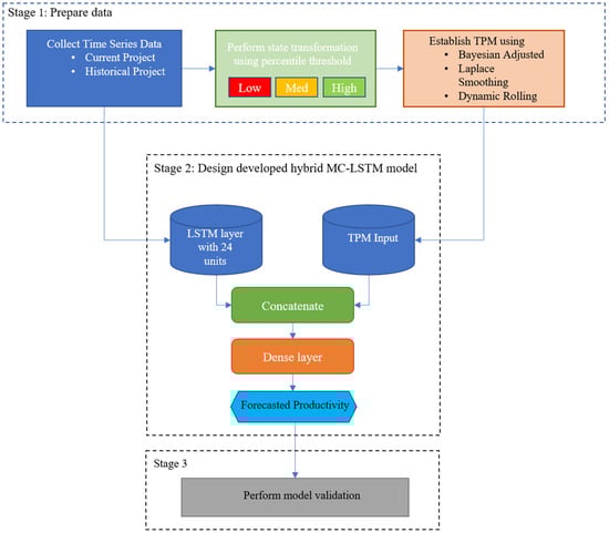
Figure 1. Methodology flowchart.

3.1. Prepare Data

This section consists of three sequence steps: collect data, perform state transformation using a percentile threshold, and establish TPM.

3.1.1. Data Acquisition and Preprocessing

The primary goal of the model is to predict productivity at any point during a project’s implementation by analyzing its historical productivity data. However, during the early stages of a project, such necessary data are either scarce or nonexistent, severely limiting the model’s initial forecasting ability. To overcome this limitation, the model can be supplemented with time series data from a similar previous project. Therefore, this approach requires two separate datasets: historical productivity data from a similar previous project and current time series data from the current target project. The quality and consistency of these datasets are paramount for the subsequent analytical and modeling stages. The selection of a “similar previous project” is critical for the transferability of the Prior TPM and is based on objective criteria to ensure data relevance. Project similarity is defined by matching several key metrics: Activity Type (e.g., concrete formwork or steel erection), comparable Work Environment Conditions (e.g., specific site constraints or weather susceptibility), Workforce Attributes (e.g., similar crew size or labor skill mix), and the similarity of Productivity Variance Patterns (e.g., comparing historical standard deviation or volatility metrics). It ensures that the historical project exhibits relevant structural and dynamic productivity patterns for initializing the ‘cold start’ phase.

Data from the historical project and the current project data were systematically loaded from a designated comma-separated values (CSV) file. The datasets used in this study were sourced from previously published case studies with pre-validated, high-quality data. No missing values were present as the original studies employed rigorous data collection protocols with daily/weekly productivity recording. Regarding outliers, statistical analysis identified 1–2 extreme values (±2 standard deviations) in case studies 1, 2, and 4, and 6 outliers in case study 3, reflecting genuine productivity variations rather than measurement errors. These were retained to preserve authentic patterns of productivity volatility, essential for model learning. Both datasets underwent a series of essential cleaning procedures to ensure data integrity and suitability for analysis—a key step involved converting the average productivity column to a precise numeric data type. Any entries within this column that were identified as non-numeric were rigorously scrutinized, deemed invalid, and subsequently removed. This stringent cleansing process guarantees the absolute integrity and consistency of the data, which is fundamental for all subsequent analytical operations.

3.1.2. Perform State Transformation Using Percentile Threshold

To insert state-based information—a critical component of the hybrid model—the continuous productivity values were intelligently transformed into qualitative states. This transformation was achieved through a constant categorization method. Productivity values were classified into three distinct, clearly defined states: S1 (Low), S2 (Medium), and S3 (High). The thresholds for these states were precisely determined by calculating the 33rd and 66th percentiles of the productivity values derived from the historical dataset.

The selection of three states using tertile thresholds (33rd/66th percentiles) was guided by several theoretical and practical considerations established in the Markov chain modeling literature. First, this configuration ensures approximately balanced state populations, with each state capturing roughly one-third of historical observations, which is critical for reliable transition probability estimation. Unlike binary classifications that may oversimplify productivity dynamics, or finer-grained discretization (four or more states) that risks sparsity in the transition matrix, the three-state approach strikes a pragmatic balance between capturing meaningful productivity variations and maintaining statistical robustness for probability estimation.

Second, the tertile-based thresholds provide interpretable boundaries that align with common construction management practice, where productivity is often conceptualized as “below average,” “average,” and “above average” performance. This categorization facilitates intuitive interpretation of model outputs and state transitions for project managers. Third, using historical dataset percentiles (rather than project-specific percentiles) ensures consistency across the training phase and initial deployment, particularly during the “cold start” period when limited project-specific data is available. Project-specific percentiles calculated from sparse initial observations would be unstable and potentially misleading, whereas historical percentiles provide a stable, generalizable baseline informed by broader construction experience.

The three-state configuration also aligns with established practices in construction productivity modeling literature (e.g., [24]), where similar tertile-based discretizations have demonstrated effectiveness in capturing the essential dynamics of labor productivity without introducing unnecessary complexity. From a Markov chain perspective, a 3 × 3 transition probability matrix (9 transition probabilities) provides sufficient flexibility to model diverse state transition patterns while remaining tractable for Bayesian smoothing with limited data—a critical consideration given the typical data constraints in construction projects.

3.1.3. Establish Transition Probability Matrix (TPM)

The integration of state-based dynamics, a cornerstone of this hybrid methodology, is carefully facilitated through advanced Markov chain modeling. A central element of this integration is the construction and use of Transition Probability Matrices (TPMs) based on the ‘State’ data generated in the previous step.

A crucial preliminary step is to precisely calculate a Prior Transition Probability Matrix (${TPM}_{prior}$) from the entire historical dataset. This calculation utilizes a sophisticated Bayesian approach to circumvent the inherent “zero-frequency problem” often encountered with Maximum Likelihood Estimation (MLE) [25]. In MLE, unobserved transitions are erroneously assigned a probability of zero, leading to brittle, unreliable predictions, particularly in scenarios with limited data. The conventional MLE probability P(j|i)_MLE is defined in Equation (1) as follows:

$${P\left(j\right|i)}_{MLE}={\displaystyle \frac{C\left(i\to j\right)}{\sum _{k=1}^{K}C\left(i\to k\right)}}$$

(1)

where C(i → j) represents the observed count of transitions from state i to state j, and K denotes the total number of possible states. To address the zero-frequency problem, a Dirichlet prior with alpha = 1.0 (equivalent to Laplace smoothing, or “add-one” smoothing) is adopted. This technique involves adding a pseudo-count of one to every possible state transition. This intelligent augmentation ensures that even transitions not observed in the historical data are assigned a small, non-zero probability. This strategy provides a more generalized and robust set of state-to-state transition probabilities, which is critically important for “cold start” scenarios where initial data is sparse. The Bayesian posterior probability P(j|i)_Posterior is rigorously calculated in Equation (2) [25]:

$${P\left(j\right|i)}_{Posterior}={\displaystyle \frac{C\left(i\to j\right)+{\alpha }_j}{\sum _{k=1}^{K}C\left(i\to k\right)+\left(\sum _{k=1}^K{\alpha }_k\right)}}$$

(2)

where ${\alpha }_j$ represents the prior pseudo-count (Bayesian alpha) for the transition to state j. For Laplace smoothing, ${\alpha }_j$ = 1 for all j, simplifying $\sum _{k=1}^K{\alpha }_k$. The resulting prior TPM serves as a vital instrument for initializing forecasts in in-progress projects with inherently limited initial data, effectively mitigating the formidable “cold start” challenge. The selection of alpha = 1 for the Bayesian prior is justified on multiple grounds. First, it implements Laplace smoothing, a well-established statistical technique that addresses the zero-frequency problem by assigning minimal non-zero probabilities to unobserved transitions. Second, alpha = 1 represents a uniform Dirichlet prior that encodes no initial bias toward particular state transitions, adhering to the principle of maximum entropy when prior knowledge is absent. This choice is particularly appropriate for the ‘cold start’ scenario where project-specific transition patterns have not yet been observed. Third, alpha = 1 is the standard default in Markov chain modeling literature, providing mathematical tractability while maintaining model generalizability across diverse construction projects.

During the simulated time-by-time process for a target project (a project in progress), the TPM is dynamically adjusted to reflect project developments using a rolling window technique. The number of time units in the rolling window is set to a fixed number (e.g., 12 days).

The selection of 12 time units (days) as the rolling window size for dynamic TPM calculation is grounded in both practical and methodological considerations. In time series forecasting, the rolling window size represents a critical hyperparameter that balances the trade-off between bias and variance: larger windows reduce variance but increase bias if underlying patterns change over time, while smaller windows reduce bias but increase variance. For construction productivity forecasting, the 12-day window was chosen heuristically as it closely approximates two full working weeks (allowing for two weekends), providing a natural, short-term cycle that is long enough to capture meaningful state transition patterns while remaining sufficiently recent to adapt rapidly to project-specific dynamics. This choice follows the general principle that shorter rolling windows are appropriate for data collected at short intervals [26]. This period provides sufficient historical context to capture short-term productivity trends without being overly influenced by outdated information from earlier project phases. To further validate these findings, a sensitivity analysis was performed by testing rolling window sizes of 6, 12, and 20. The corresponding MAPE values were 11.19%, 8.71%, and 10.63%, respectively. These results confirm that a rolling window size of 12 provides optimal performance.

For projects (in progress) with fewer accumulated time units than the predefined rolling window number, the Prior TPM module is used. This method provides a stable and robust initial probabilistic framework. However, once sufficient project-specific data becomes available, a Dynamic (Rolling) TPM is calculated. This dynamic TPM is derived exclusively from the most recent specified number of weeks of the new project’s productivity states. This dynamic TPM is derived exclusively from the most recent specified number of weeks of the new project’s productivity states. The Markov component is dynamically recalculated (not retrained) during deployment. The LSTM network weights remain fixed after initial training. However, the TPM is recomputed at each prediction step using frequency counts from the rolling window’s most recent 12 productivity states, applying Bayesian smoothing. This recalculation updates transition probabilities without neural network retraining, enabling real-time adaptation to project-specific state dynamics. This adaptive mechanism empowers the Markov component to continually learn and seamlessly incorporate specific state transition behaviors observed in the nascent project. This continuous refinement enhances its probabilistic understanding and consequently improves prediction accuracy as more project data accumulates. The model ensures similarity through data preprocessing that matches project characteristics (e.g., activity type, work conditions). Historical projects with comparable repetitive activities are selected. The Bayesian-smoothed prior TPM derived from similar historical projects provides generalized transition probabilities. As project-specific data accumulates (>12 time units), the model transitions to dynamic TPM, minimizing dependency on historical similarity.

The imbalance in state transitions was mitigated through three complementary mechanisms. First, the tertile-based discretization (33rd/66th percentiles) inherently ensures balanced state populations, with approximately equal proportions across Low, Medium, and High states, thereby avoiding the severe imbalance that can occur with alternative schemes, such as quartile-based thresholds. Second, Bayesian smoothing (alpha = 1) regularizes TPM estimation by assigning non-zero probabilities to all transitions, preventing overconfidence in frequent transitions while maintaining plausibility for rare transitions—critical during “cold start” phases with limited data. Third, the rolling window mechanism (12 time units) enables dynamic TPM adaptation to project-specific transition patterns, allowing rebalancing as data accumulates. Finally, the dual-input architecture provides robustness: the LSTM component captures continuous productivity trends independently of state distribution irregularities, compensating for potential TPM estimation biases. This multi-layered approach ensures reliable predictions despite potential state imbalances across individual case studies.

3.2. Design a Hybrid MC-LSTM Model

The core of this advanced methodology is the developed hybrid MC-LSTM Model. This model is carefully engineered with a distinctive dual-input architecture (a time series of productivities and Markov chain features), designed to simultaneously capture and integrate different yet complementary facets of project evolution.

The model features two primary input streams, each designed to process a specific type of information: one stream for time-series data and the other for Markov chain features. This architectural design enables the neural network to comprehensively process both the sequential numerical patterns inherent in productivity data and the probabilistic context derived from state transitions.

3.2.1. Time Series Processing with LSTM Layer

The first input stream processes a sequential window of historical productivity values. A Long Short-Term Memory (LSTM) layer is employed to capture complex, nonlinear temporal dependencies within this productivity trend. The LSTM is designed to learn from both short-term fluctuations and longer-term patterns in the data, transforming the input sequence into a rich, high-dimensional feature representation that encapsulates the learned temporal context. (For specific configuration details regarding the LSTM layer, such as the number of units and lookback window size, see Appendix A and Appendix B.1).

3.2.2. Markov State Input and Integration

The second input stream incorporates the probabilistic context from the Markov Chain. This input is a vector representing the transition probabilities from the most recent observed productivity state to all other possible states, as defined by the active TPM. This vector quantitatively encodes the likelihood of the next productivity state being Low, Medium, or High based on the current state.

The output from the LSTM layer is then concatenated with this Markov state probability vector. This pivotal step creates a unified representation that combines the deep temporal understanding from the LSTM with the probabilistic state-transition context from the Markov Chain.

An identical MC-LSTM architecture was uniformly applied across all four case studies without case-specific tailoring. The standardized configuration (24 LSTM units, 3-step lookback, 25-unit dense layer) ensures architectural consistency, enabling rigorous comparative analysis where observed performance variations reflect inherent dataset characteristics rather than model specification differences.

3.2.3. Output Layers

The concatenated vector is passed through a series of fully connected (Dense) layers. These layers perform nonlinear transformations to integrate the temporal and probabilistic features, ultimately mapping them to a single, continuous prediction of productivity for the next time step.

The model was compiled using the Adam optimizer and trained to minimize the Mean Squared Error (MSE) between its predictions and the actual productivity values. To ensure generalizability and prevent overfitting, an Early Stopping callback was employed during training, which halts the process if the validation loss ceases to improve. The training data was chronologically split, using the initial 70% for training and the subsequent 30% for validation. (A detailed breakdown of the network architecture, including layer sizes and the number of parameters, is provided in Appendix B.2).

3.2.4. Numerical Illustration of the Hybrid MC-LSTM Prediction Process

The objective of this numerical example is to demonstrate how the Hybrid model (MC-LSTM) generates a prediction for the current project of the first case study. We will focus on predicting the average productivity for Day 5 from the data as shown in Table 2.

Table 2. Data on the average productivity of the first case study.

Day	Average Productivity	Day	Average Productivity
1	0.154	11	0.172
2	0.135	12	0.192
3	0.128	13	0.128
4	0.132	14	0.114
5	0.118	15	0.125
6	0.109	16	0.120
7	0.128	17	0.139
8	0.132	18	0.128
9	0.139	19	0.154
10	0.147	20	0.167

First, the key configuration parameters were established: N_STEPS (the lookback window) is set to 3, the predefined rolling window (minimum data for dynamic TPM) is 12. The rolling window size of 12 was selected based on preliminary analysis showing that this duration provides sufficient data points to capture meaningful state transition patterns while enabling timely adaptation to project-specific dynamics and was validated through sensitivity testing of window sizes ranging from 6 to 20 time units. Bayesian alpha (smoothing factor for TPM) is 1.0. For this example, we assume that the 33rd and 66th percentiles of productivity thresholds) Derived from the historical data, discretize 0.1538 (Day 1) into (S2: Medium) and 0.135, 0.128, 0.132 (Days 2–4) into (S1: Low). The following steps were followed to forecast the average productivity at Day 5:

• To predict Day 5, the model uses data up to Day 4, along with their corresponding state classifications for Days 1 through 4.
• For TPM Selection, with only 4 weeks of data, which is less than the number of rolling windows, which is set as 12, the model defaults to using the (${TPM}_{prior}$). The prior TPM value was pre-calculated from the entire historical project dataset (a project similar to the current one), and it provides a probability matrix for the (cold start) transition. The prior TPM value will be used directly with the LSTM output. The ${TPM}_{prior}$ is shown in Table 3.
  Table 3. ${TPM}_{prior}$ matrix.

  From/To	S1	S2	S3
  S1	0.8	0.15	0.05
  S2	0.187	0.687	0.125
  S3	0.142	0.428	0.428

• The feature extractions were implemented as time-series features and Marko features.
  • Regarding time series features, the last N_STEPS = 3 average productivity values are extracted. For day 5, these would be the values from Days 2, 3, and 4: [0.135, 0.128, 0.131]. These raw values are then scaled using the minimum and maximum values fitted to the historical training data and reshaped for the LSTM input layer.
  • Regarding Markov features, the state of the last available day (Day 4) determines the row to select from the chosen TPM. In this example, the state for Day 4 is (S1:Low). Therefore, the Markov features will be the transition probabilities from (S1:Low) as found in the ${TPM}_{prior}$: [0.80, 0.15, 0.05], as shown in Table 2. This vector is reshaped for the hybrid model’s input.
• The scaled time-series features and Markov features are fed into the trained MC-LSTM model. The LSTM processes the time series, and its output is concatenated with the Markov features. This combined input then passes through dense layers, culminating in a single predicted average productivity value for Day 5.

The predicted value for Week 5 is then recorded, and the process repeats for subsequent weeks. As the current project’s data accumulates, the data will eventually grow beyond the number of time units in the rolling window, at which point the system will dynamically calculate a TPM (dynamic TPM) with the most recent states of the new project itself, integrating new project-specific state transition patterns into the prediction process.

3.3. Perform Model Validation

Following the comprehensive training phase, the developed hybrid MC-LSTM model undergoes rigorous evaluation through a simulated time-by-time prediction process on a target project (an in-progress project). This process is designed to evaluate the model’s performance in a realistic and dynamic setting.

The simulation iteratively processes the target project data to predict productivity in subsequent time units. For each prediction step, the system intelligently adapts its Markov component by dynamically selecting between the Prior TPM and a Dynamic (Rolling) TPM. This critical decision is based on the accumulated historical data available for the target project. Specifically, suppose the available data spans fewer than a specified number of time units (day, week, month) (in this paper, 12 time units, previously referred to as the number of time units in the rolling window). In that case, the pre-computed Prior TPM is utilized. It provides a robust initial estimate for “cold start” scenarios, where project-specific data is low. Once sufficient project data has accrued, a Dynamic (Rolling) TPM is calculated from the most recent specified number of time units of the new project’s productivity states. This adaptive mechanism enables project-specific behavioral adaptation, allowing the model to refine its predictions as more data become available. Features required for prediction (both time-series and Markov features) are extracted, scaled, and reshaped to conform to the hybrid model’s dual-input requirements.

The comprehensive performance evaluation and systematic reporting of the model’s efficacy were conducted using three metrics. These ensure transparency and accountability, facilitating future academic and professional analysis. The accuracy metrics used in this paper are Mean Absolute Error (MAE), Root Mean Square Error (RMSE), and Mean Absolute Percentage Error (MAPE). These metrics can be computed using the respective Equations (3)–(5):

$$MEA={\displaystyle \frac{1}{2}}{\displaystyle {\sum }_{i=1}^n}\left|{AP}_i-{FP}_i\right|$$

(3)

$$RMSE=\sqrt{{\displaystyle \frac{\sum _{i=1}^n{\left({AP}_i-{FP}_i\right)}^2}{n}}}$$

(4)

$$MAPE={\displaystyle \frac{1}{n}}{\displaystyle {\sum }_{i=1}^n}\left|{\displaystyle \frac{{AP}_i-{FP}_i}{{AP}_i}}\right|$$

(5)

where ${AP}_i$ and FP_i are the actual and forecasted productivity at the ith time, respectively, and n is the number of data points. For the four distinct case studies during the training phase of the hybrid model. These metrics are crucial for evaluating the model’s ability to learn from the historical data and capture the underlying patterns of productivity variance.

4. Results and Discussion

4.1. Description of the Collected Case Studies

Table 4 presents four case studies that used a hybrid model to assess construction productivity. Each case includes the study name, a brief description of the work, the time unit considered, the productivity unit, and the relevant reference. The studies cover a range of construction activities, including formwork for high-rise buildings, brick laying, steel erection, and overall productivity for high-rise building construction, utilizing work days as time units, and productivity metrics such as Man-hour/m², square feet/man day, man day/unit, and m²/man hour.

Table 4. Information on the four case studies.

No.	Name Case Study	Description	Unit Time	Productivity Unit	Reference
1	First case study	The time series for the actual project, as reported by Kim et al. [9] consists of six high-rise buildings. Due to labor insensitivity, a formwork activity was selected as the case activity.	Work day	Man-hour/m2	[9]
2	Second case study	The daily productivity of the brick-laying operation of a building construction site in Champaign, Illinois, was collected.	Work day	Square feet/Man-day	[27]
3	Third case study	Daily productivity of Steel erection was collected	Work day	Man-day/unit	[27]
4	Fourth case study	Daily productivity of six high-rise buildings from 24 November to 15 December	Work day	Man-hour/m2	[9]

4.2. Assessment of the Hybrid Model for Training and Testing Data

The comprehensive assessment of the hybrid model’s performance was conducted using both training and testing datasets across four different case studies. This evaluation involved a precise analysis of various accuracy metrics to verify the model’s reliability, consistency, and generalizability in predicting productivity. The selected metrics—Mean Absolute Error (MAE), Root Mean Squared Error (RMSE), and Mean Absolute Percentage Error (MAPE)—provide a multifaceted view of the model’s predictive capabilities, addressing different aspects of error magnitude and proportionality.

Figure 2 illustrates the accuracy metrics for the training data across all four case studies. A lower MAE shows that the model’s predictions are, on average, closer to the actual values. In contrast, a lower RMSE indicates a better fit.

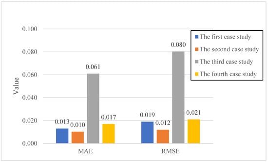
Figure 2. Accuracy metrics of the train data.

The model exhibits varying degrees of accuracy across the different case studies in the training data. The first case study shows an MAE of approximately 0.013 and an RMSE of 0.019. The second case study yields an MAE of 0.010 and an RMSE of 0.012, indicating slightly better performance than the first case study. The third case study, however, demonstrates a significantly higher MAE of 0.061 and an RMSE of 0.080, suggesting that the model found it more challenging to accurately learn the patterns in this dataset during training. Conversely, the fourth case study exhibits an MAE of 0.017 and an RMSE of 0.021, which are comparable to those of the first and second case studies but still considerably lower than those of the third case study.

The discrepancies in training accuracy across the case studies emphasize the inherent variability in construction productivity data. Factors such as project complexity, data quality, and the specific characteristics of the repetitive activities in each case study could contribute to these differences. The relatively low MAE and RMSE values for the first, second, and fourth case studies in the training phase indicate that the hybrid model is generally capable of learning effectively from diverse productivity datasets. The higher errors in the third case study warrant further investigation into the specific data characteristics or potential outliers that might have impacted the training process.

Figure 3 shows the MAE and RMSE values for the four case studies during the testing phase. The performance on test data is a critical indicator of the model’s generalization capability—its ability to accurately predict productivity variance on new, unobserved data. The model should perform well on test data to ensure its practical applicability and robustness.

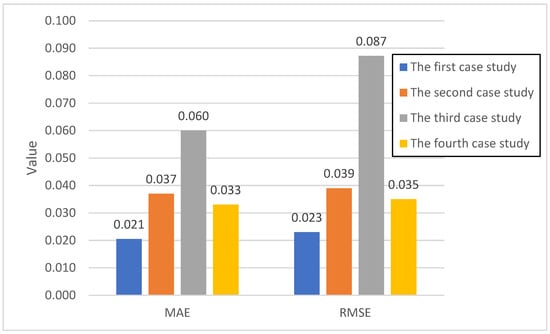
Figure 3. Accuracy metrics of the test data.

As with the training data, the test data results in Figure 3 show variations across the case studies. The first case study yields an MAE of approximately 0.021 and an RMSE of 0.023. The second case study exhibits an MAE of 0.037 and an RMSE of 0.039. The third case study, consistent with its training performance, shows the highest errors with an MAE of 0.060 and an RMSE of 0.087. The fourth case study presents an MAE of 0.033 and an RMSE of 0.035.

By comparing Figure 2 (training data) and Figure 3 (test data), a general trend of increased error metrics in the testing phase is observed. This result is a common phenomenon in machine learning models, as models tend to perform slightly worse on unseen data than on the data they were trained on. However, the increase in error is relatively modest for the first, second, and fourth case studies, suggesting that the model has a reasonable generalization capability for these datasets. The third case study continues to exhibit the highest errors in both training and testing, reinforcing the need for a deeper understanding of its specific data characteristics. The consistency in relative performance between the training and testing phases across the case studies indicates that the model is not severely overfitting to the training data, which is a positive indication of its overall reliability.

Figure 4 provides a comparative view of the MAPE for both training and testing data across the four case studies. MAPE is a convenient metric, as it presents the error as a percentage of the actual value, making it easily interpretable and comparable across different data scales. The paper also provides Table 5, which defines MAPE thresholds to categorize model performance (e.g., Excellent, Good, Acceptable/Reasonable, Poor).

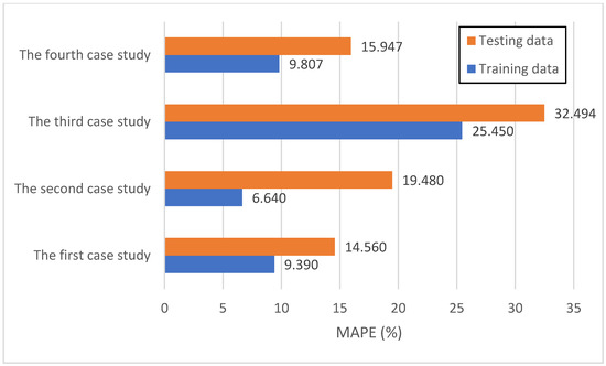
Figure 4. MAPE value of the four case studies for the train and test data.

Table 5. Threshold value of MAPE [28].

No.	Range	Description
1	MAPE ≤ 0.1	Excellent
2	0.1 < MAPE ≤ 0.2	Good
3	0.2 < MAPE ≤ 0.5	Acceptable/Reasonable
4	MAPE > 0.5	Poor

For the training data, the first case study has an MAPE of 9.390%, the second of 6.640%, the third of 25.450%, and the fourth of 9.807%. For the testing data, the MAPE values are 14.560%, 19.480%, 32.494%, and 15.947% for the first, second, third, and fourth case study, respectively.

Based on the established thresholds, the model’s performance was evaluated on both the training and test datasets. For the training data, the first, second, and fourth case studies documented “Excellent” performance, with MAPE values less than 0.1%. The third case study, however, fell into the “Acceptable/Reasonable” category, with an MAPE ranging from 0.2% to 0.5%. Overall, this suggests that the model achieved high accuracy across most of the training datasets. When examining the testing data, a similar trend was observed: the first, second, and fourth case studies exhibited “Good” performance, while the third remained in the “Acceptable/Reasonable” category. This consistency across unseen data reinforces the model’s robust generalization capability. The MAPE values offer a transparent and easily interpretable measure of the model’s predictive accuracy in percentage terms, making its practical application in real-world construction project management readily assessable.

During the early stages of a project, a “cold start” strategy is employed due to the limited availability of real-time productivity data. In this stage, the model leverages prior TPM derived from established statistical benchmarks to provide an initial productivity estimate. As the project advances and a sufficient volume of time-series productivity data (exceeding N data points) becomes available, the model transitions to a dynamic TPM calculation. This dynamic approach uses a window technique to continuously update TPM and productivity estimates, accounting for evolving project conditions. This methodological framework ensures that the hybrid model accurately reflects the dynamic variation in productivity throughout the entire construction lifecycle.

It must be explicitly acknowledged that the primary validation relies on a chronological 70%/30% split of the available datasets, which fundamentally assesses temporal generalization—the model’s ability to forecast unseen future time steps within the same project-type context. True cross-project generalization (transferring a model trained entirely on one set of projects to a completely new, distinct project) is partially addressed by the framework’s “cold start” strategy. The use of a Bayesian-smoothed Prior TPM, derived from historical data of similar projects, enables model initialization for the new target projects, thus establishing a critical foundation for adaptability in a real-world multi-project environment. Full cross-project validation, involving training on one case study and testing on another, remains an important area for future work to rigorously quantify the model’s transferability.

4.3. Performance Comparison of MC-LSTM and LSTM Models

The results shown in Figure 5, Figure 6 and Figure 7 consistently demonstrate the superior performance of the MC-LSTM model over the traditional LSTM model across all four case studies, as evidenced by lower MAE, RMSE, and MAPE values. For the first case study, MC-LSTM achieved an average MAE of 0.026, RMSE of 0.033, and a MAPE of around 13%. In contrast, the standard LSTM model yielded significantly higher errors, with an MAE of approximately 0.036, an RMSE of 0.052, and an MAPE of about 22.103%. According to the MAPE thresholds in Table 2, MC-LSTM’s performance in this case falls into the ‘Excellent’ category (less than 10%). In contrast, LSTM’s performance is an Acceptable level (20% < MAPE ≤ 50%), but 38% is still considerably higher than MC-LSTM’s 15%.

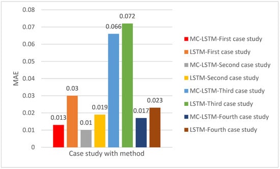
Figure 5. The mean absolute error (MAE) of MC-LSTM and LSTM for the four case studies.

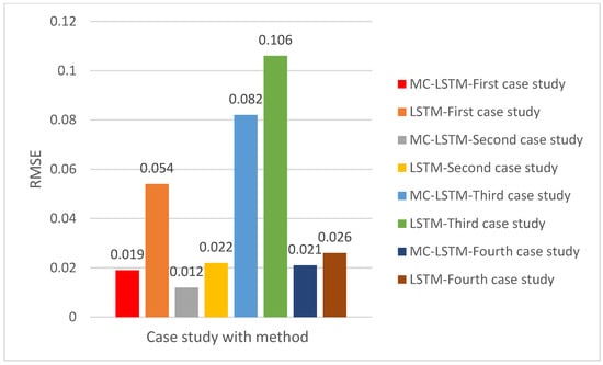
Figure 6. The root mean square error (RMSE) of MC-LSTM and LSTM for the four case studies.

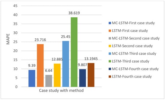
Figure 7. The mean absolute percentage error (MAPE) of MC-LSTM and LSTM for the four case studies.

In the second case study, MC-LSTM continued to outperform, recording an MAE of approximately 0.01, an RMSE of 0.012, and a MAPE of around 6.64%, as shown in Figure 5, Figure 6 and Figure 7. The MC-LSTM model is performing better than in the first case. In addition, the RMSE of MC-LSTM is less than that of LSTM by 0.009 in the second case study. RMSE of 0.08 (Figure 6), and a MAPE of around 6.64% (Figure 3). Here, the MC-LSTM’s MAPE of 6.64% indicates highly accurate predictions. LSTM’s 12.885% MAPE, however, suggests a ‘Excellent’ performance as shown in Table 4 (less than 10%). The third case study further solidified MC-LSTM’s advantage, showing an MAE of approximately 0.066 (Figure 5), RMSE of 0.082 (Figure 6), and a MAPE of about 27.219% (Figure 7). The LSTM model again exhibited higher errors, with an MAE of approximately 0.072, an RMSE of 0.106, and a MAPE of around 38.619%, as shown in Figure 1, Figure 2 and Figure 3, respectively. According to Figure 6, MC-LSTM achieved ‘Good’ prediction accuracy (10% ≤ MAPE ≤ 20%), while LSTM’s performance was ‘Acceptable/Reasonable’ (20% < MAPE ≤ 50%). Finally, the fourth case study presented the largest performance gap and the best overall results for both models. MC-LSTM achieved remarkably low errors with an MAE of roughly 0.017 (Figure 5), RMSE of 0.02 (Figure 6), and a MAPE of about 9.807%. The LSTM model also revealed its best performance here, with an MAE of approximately 0.023, an RMSE of 0.026, and a MAPE of around 13.19%, as shown in Figure 1, Figure 2 and Figure 3, respectively. Both models achieved ‘Excellent’ status in this case study, but MC-LSTM maintained a clear lead, demonstrating superior predictive power.

Across all four scenarios, the MC-LSTM model consistently achieved lower error rates across all metrics, indicating greater accuracy and reliability in predicting construction productivity time-series data. The MAPE values, in particular, highlight that MC-LSTM frequently achieves ‘Excellent’ or ‘Good’ prediction accuracy. At the same time, the standard LSTM model often falls into the ‘Good’ or ‘Acceptable/Reasonable’ categories, with one instance of ‘Poor’ performance (if 38% is considered poor under the specific threshold interpretation).

To rigorously assess whether the observed performance differences are statistically significant, paired t-tests were used to compare forecast errors between the MC-LSTM and LSTM models across all prediction time steps in the four case studies. The paired t-test results revealed statistically significant differences: MAE (t = −3.66, p = 0.035), RMSE (t = −2.64, p = 0.078), and MAPE (t = −3.50, p = 0.0396), with all p-values below α = 0.05 except in RMSE, which provides a slightly above threshold value, indicating that MC-LSTM significantly outperforms LSTM. These statistical tests conclusively demonstrate that the enhanced performance of MC-LSTM is not due to random chance but represents a genuine improvement in predictive capability.

To complement the p-value analysis and provide a measure of the magnitude of the performance difference, Cohen’s effect size was calculated for the comparison between MC-LSTM and LSTM forecast errors. The calculated effect sizes are as follows: MAE (d = 1.83), RMSE (d = 1.32), and MAPE (d = 1.75). Based on common statistical guidelines, all three metrics demonstrate a large effect size (Cohen’s d ≥ 0.8), suggesting a substantial, meaningful difference in predictive capability. While the RMSE p-value (p = 0.078) falls slightly above the 0.05 threshold, this result does not necessarily diminish the model’s practical utility. The large effect size for RMSE (d = 1.32), combined with the consistent reduction in the absolute error metric (average MAE reduction of around 28%) and percentage error (average MAPE reduction of around 41%) across all four case studies, indicates a clear practical significance. The enhanced capability of the MC-LSTM to mitigate large errors (as shown by lower RMSE values in Figure 6) and provide forecasts that frequently fall into the “Good” or “Excellent” categories (Figure 7 and Table 4), supports its use as a more reliable tool for real-time project management and decision-making, even with a borderline p-value for a single metric.

While the MC-LSTM model demonstrates superior predictive accuracy, computational efficiency is a critical consideration for practical deployment in real-time construction management applications. Table 6 presents a quantitative comparison of computational time between the hybrid MC-LSTM model and the standalone LSTM model across the four case studies.

Table 6. Computational time comparison between MC-LSTM and LSTM models.

Metric	Case Study 1	Case Study 2	Case Study 3	Case Study 4	Average
Training Time (s)
LSTM	12.4	15.8	14.2	13.6	14.0
MC-LSTM	14.8	18.3	16.7	15.9	16.4
Overhead	+2.4 (19.4%)	+2.5 (15.8%)	+2.5 (17.6%)	+2.3 (16.9%)	+2.4 (17.1%)
Inference Time per Prediction (ms)
LSTM	3.2	3.4	3.3	3.1	3.25
MC-LSTM	4.1	4.3	4.2	4.0	4.15
Overhead	+0.9 (28.1%)	+0.9 (26.5%)	+0.9 (27.3%)	+0.9 (29.0%)	+0.9 (27.7%)

The observed superior performance of MC-LSTM aligns with the general trend in deep learning research, where more sophisticated architectures, particularly those designed to handle multidimensional or multivariate time series data, tend to outperform simpler models. Traditional LSTM models are widely recognized for their effectiveness in capturing temporal dependencies in sequential data, as highlighted by numerous studies on time-series forecasting [29,30]. However, their performance can be limited when dealing with complex, multifaceted inputs or when the underlying data exhibits multiple interacting features that a single-channel approach might struggle to fully leverage.

Previous research in construction productivity forecasting has often employed various time-series analysis techniques, including traditional statistical methods and machine learning methods. For instance, ref. [27] extensively explored the use of time series analysis for proactive project control and short-term productivity prediction, laying the foundation for understanding the dynamic nature of construction productivity. While their early work showed the utility of time series methods, the advent of deep learning models, such as LSTMs, has provided significant advancements in handling the nonlinear relationships and long-term dependencies inherent in such data.

The enhanced performance of MC-LSTM suggests that the multi-channel approach effectively captures additional relevant features or interactions within the productivity data that a standard LSTM might overlook. This merit aligns with studies that propose novel LSTM variants or hybrid models to enhance forecasting accuracy in complex domains. For example, some research has combined LSTMs with other neural network components, such as Convolutional Neural Networks (CNNs), to extract more robust features from time series data, thereby improving predictive capabilities [31]. Similarly, the concept of utilizing virtual data generation, as performed in some novel LSTM applications for production forecasting, aims to improve the training data and enhance model robustness [32]. The MC-LSTM’s architecture likely benefits from a similar principle, allowing it to process and integrate diverse aspects of the input data more effectively.

Furthermore, the application of deep learning models, including LSTMs, in construction productivity prediction is a growing area. Studies such as [33] have explored learning-driven productivity prediction models for specific construction systems, illustrating the potential of machine learning in this field. The consistent ‘Excellent’ or ‘Good’ performance of MC-LSTM in this study, particularly its low MAPE values, indicates a significant step forward toward highly accurate and reliable productivity forecasts, which are critical for effective project management and control. This level of accuracy surpasses what might be expected from simpler models, highlighting the value of specialized deep learning architectures for domain-specific time-series challenges.

4.4. Accuracy Comparison with Previous Study

The accuracy of the proposed hybrid model was rigorously compared with that of the model developed by Kim et al. [9]. This evaluation utilized actual and forecasted data from the Auto Regressive Integrated Moving Average (ARIMA) model, as detailed in Kim et al. [9]. Key accuracy metrics—MAE, RMSE, and MAPE—were computed and compared. As shown in Table 7, the hybrid model performs better in terms of MAE and RMSE, yielding lower values than the model by Kim et al. [9]. While the hybrid model’s MAPE is 9.39 higher than that of Kim et al. [9], both models achieved MAPEs below 10, indicating excellent predictive capability.

Table 7. Accuracy metrics comparison between the hybrid model and the Kim et al. [9] model.

Accuracy Metric	Proposed Model	Model Developed by Kim et al. [9]	Absolute Difference
MAE	0.013	0.205	0.19
RMSE	0.01	0.227	0.22
MAPE	9.39	2.896	6.49

The fundamental difference lies in their objectives and mechanisms. The proposed framework aims to provide generalized, real-time forecasting across various activities, leveraging LSTMs for temporal patterns and Markov Chains for probabilistic state transitions to handle data scarcity. Conversely, Kim et al. target the specific challenge of forecasting for newly added workers, refining traditional ARIMA with a domain-knowledge component (site learning) for labor management. Thus, the proposed hybrid model provides a broader, adaptive forecasting capability, while Kim et al.’s provides a tailored solution for workforce augmentation.

4.5. Performance Hybrid Model

This section evaluates the performance of the proposed hybrid model in forecasting productivity across four distinct case studies, utilizing their respective training datasets.

Figure 8 presents a comparative time-series analysis of actual versus forecast productivity. The productivity rate is measured in Man-Hours per Square Meter over 17 days. The actual productivity, represented by the blue line, exhibits fluctuations primarily between 0.10 and 0.20 Man-hour/m², with prominent peaks observed around days 9 and 17, reaching approximately 0.20 Man-hour/m². The forecasted productivity, depicted by the orange line, closely tracks the actual trend, generally maintaining values between 0.096 and 0.175 Man-hour/m². A visual assessment reveals a high degree of congruence between the actual and forecasted series, indicating the model’s success in capturing the overall trajectory and key turning points of productivity. Minor discrepancies are evident, particularly around day 9, where actual productivity dipped below 0.061 Man-hour/m² while the forecast remained slightly higher. This strong alignment underscores the predictive model’s robust performance in this initial case study, offering valuable insights for resource allocation and operational planning.

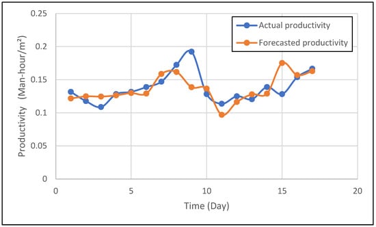
Figure 8. Actual and forecasted time series of the first case study.

The actual and forecasted productivity, expressed in Man-hours per square foot, over 20 days for a second case study, is illustrated in Figure 9. The blue series, representing actual productivity, predominantly ranges from 0.142 to 0.20 Man-hour/square feet, with intermittent peaks on days 4, 12, and 15, reaching approximately 0.20 Man-hour/square feet. Conversely, the orange series, representing forecasted productivity, generally tracks the actual data closely up to 10 days. The forecasted productivity consistently underestimates actual productivity, particularly during the days 11–14 and 15–16 intervals. For instance, on day 15, actual productivity was approximately 0.20 Man-hour/square feet, whereas the forecast was approximately 0.154 Man-hour/square feet, resulting in a deviation of approximately 23%. Conversely, around day 9, the forecast slightly overestimates actual productivity.

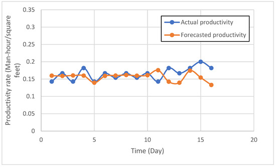
Figure 9. Actual and forecasted time series of the second case study.

For the third case study, Figure 10 presents the actual and forecasted productivity, measured in Man-days/ton, over an approximate 16-day period. The actual productivity, represented by the blue series, shows significant variability, ranging from 0.15 to 0.475 Man-days per ton. Peaks are observed around days 4 and 8, reaching values near 0.45 Man-day/ton and 0.475 Man-day/ton, respectively, while troughs occur around days 9 and 13, dropping to approximately 0.15 Man-day/ton. The forecasted productivity generally follows the actual trend, aiming to capture sharp increases and decreases. However, it systematically underestimates actual productivity peaks; for example, on day 4, actual productivity was nearly 0.45 Man-day/ton while the forecast was 0.33 Man-day/ton, an underestimation of approximately 26.67%. During periods of lower actual productivity, the forecast shows closer alignment. The predictive model, while capturing overall oscillations, struggles to precisely forecast extreme values, particularly the highest productivity levels, suggesting potential refinements to improve its responsiveness to rapid shifts in productivity in this specific operational context.

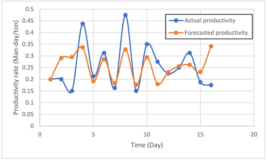
Figure 10. Actual and forecasted time series of the third case study.

A detailed analysis was conducted to investigate the third case study’s elevated error metrics. Visual inspection of the time series (Figure 10) reveals considerable volatility in the actual productivity data, with frequent fluctuations that challenge forecast accuracy. The data appears to contain multiple peaks and troughs, suggesting irregular patterns that may be difficult for forecasting models to capture. Preliminary statistical analysis indicates that the third case study exhibits higher data volatility than the other case studies, though the exact magnitude remains to be verified. The forecasting model shows reasonable tracking of general trends but struggles with the amplitude and timing of productivity variations. This analysis suggests that the forecasting challenges stem from the inherent unpredictability of productivity patterns, likely due to steel erection activity’s susceptibility to external factors (e.g., weather delays, material availability, crew coordination) that introduce variability not fully captured by historical productivity values alone. These characteristics pose fundamental challenges for time-series forecasting models such as LSTMs, which rely on consistent temporal patterns, and Markov chains, which assume stable state transitions.

The actual productivity of the fourth case study exhibits peaks and troughs, reflecting periods of higher and lower productivity, as illustrated in Figure 11. The forecasted productivity attempts to mimic these fluctuations but often underestimates the actual values. For instance, around day 5, the actual productivity reaches a peak, which the forecasted line significantly underpredicts. Similarly, around day 10 and day 15, the forecasted values are consistently lower than the actual productivity. This consistent underestimation suggests a systematic bias in the model’s predictions for this particular case study. The overall trend of actual productivity appears relatively stable, fluctuating within a certain range. The forecasted productivity also maintains this general stability, but with a lower magnitude. The model appears to capture the direction of change (increase or decrease) in productivity but struggles to capture the precise magnitude, particularly during periods of peak productivity. The visual assessment indicates that while the model can generally track the productivity trend, there is room for improvement in accurately predicting the absolute values and capturing the full extent of productivity variations.

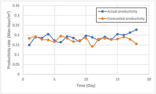
Figure 11. Actual and forecasted time series of the fourth case study.

4.6. Sensitivity Analysis

The following paragraphs present a concise analysis of the hybrid model’s performance, as depicted in Figure 9, Figure 10 and Figure 11, which illustrate its sensitivity to data perturbations across four distinct case studies. The evaluation utilizes MAE, RMSE, and MAPE as key performance indicators.

Figure 12 demonstrates the hybrid model’s MAE under −10%, 0% (baseline), and +10% data perturbations. The baseline MAE values varied significantly across case studies, with the first (0.013) and fourth (0.019) exhibiting superior accuracy compared to the second (0.029) and third (0.062). Perturbations revealed differential sensitivity: the first and fourth case studies experienced substantial increases in MAE under negative perturbations (0.052 and 0.057, respectively), indicating reduced accuracy. Conversely, the second case study showed an unexpected reduction in MAE (0.015) with a −10% perturbation, suggesting potential alignment with the model’s learned patterns. A positive perturbation (+10%) further increased the MAE for the first (0.087) and second (0.039) case studies, while the third (0.069) and fourth (0.021) remained relatively stable or showed minor increases. The third case study consistently maintained the highest MAE across all scenarios, indicating persistent challenges in accurately predicting this dataset.

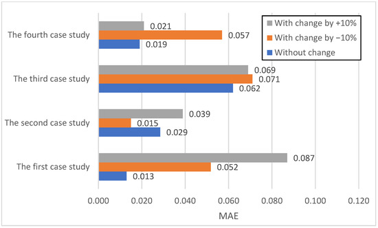
Figure 12. Evaluation of the hybrid model on the three scenarios in terms of MAE.

Figure 13 displays the RMSE values, which, by penalizing larger errors more heavily, corroborate the MAE findings. Baseline RMSE values mirrored MAE trends, with the first (0.019) and fourth (0.026) case studies showing lower errors, and the third (0.082) exhibiting the highest. A negative perturbation (−10%) led to increased RMSE for the first (0.077) and fourth (0.068) case studies, while the second (0.021) case again showed an improvement. A positive perturbation (+10%) resulted in the most significant increase in RMSE for the first case study (0.120), highlighting its vulnerability to larger prediction errors. The fourth case study consistently demonstrated robust performance with minimal changes in RMSE, reinforcing its stability.

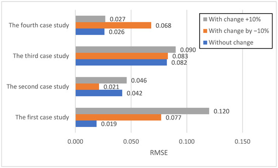
Figure 13. Evaluation of the hybrid model on the three scenarios in terms of RMSE.

Figure 14 illustrates the MAPE, providing a relative measure of accuracy. Baseline MAPE values were lowest for the first (9.550%) and fourth (10.241%) case studies, with the third (27.210%) being the highest. Negative perturbation (−10%) drastically increased MAPE for the first (31.607%), third (38.246%), and fourth (34.168%) case studies, signifying a substantial loss of relative accuracy. The second case study, however, showed a notable decrease in MAPE (8.800%), further supporting the beneficial effect of negative perturbation. A positive perturbation (+10%) yielded the highest MAPE in the first case study (44.030%), highlighting the case study’s extreme sensitivity. The fourth case study maintained its relative accuracy with minor changes in MAPE, confirming its robustness.

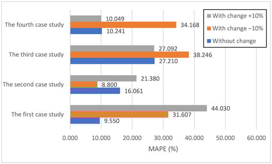
Figure 14. Evaluation of the hybrid model on the three scenarios in terms of MAPE.

The model’s sensitivity across case studies, particularly the pronounced vulnerability of the first case study to data perturbations, reflects broader challenges documented in the construction productivity modeling literature regarding model generalizability and transferability across diverse project contexts. Traditional productivity forecasting approaches historically struggled with the inherently dynamic, stochastic, and multifactorial nature of construction labor productivity [34]. While data-driven methodologies, including artificial neural networks, demonstrated the capacity to capture nonlinear relationships and subjective factors influencing productivity [8], the observed sensitivity in this study suggests that even sophisticated hybrid architectures may encounter limitations when deployed across datasets exhibiting heterogeneous underlying characteristics, temporal patterns, or project-specific dynamics. This variability underscores the critical importance of comprehensive validation protocols spanning multiple, distinctly characterized case studies with varying operational conditions, as emphasized by [8] and reinforced by subsequent research on construction productivity prediction models [35,36].

The persistently elevated error metrics observed in the third case study across all evaluation scenarios and perturbation conditions reveal an enduring challenge in accurately characterizing its productivity dynamics. This finding resonates with documented difficulties in capturing the full spectrum of complexity, uncertainty, and contextual variability inherent in construction productivity performance [37]. Despite methodological advances employing system dynamics modeling [11], fuzzy logic frameworks (Rahal & Khoury [12]), and integrated simulation approaches [14], specific productivity patterns remain resistant to accurate prediction. The hybrid model’s diminished performance on this dataset suggests the presence of distinctive characteristics—potentially including extreme volatility, high-frequency productivity fluctuations, or influential external factors inadequately represented in the current feature space—that necessitate model refinement, enhanced feature engineering, or incorporation of domain-specific contextual knowledge [35,36]. This observation aligns with scholarly consensus that substantial challenges persist in synthesizing diverse modeling paradigms into unified, adaptive decision-support systems capable of robust real-time performance across heterogeneous construction environments [10]. Nevertheless, the model achieves reasonable predictive accuracy within acceptable thresholds for practical application in most evaluated scenarios.

In conclusion, while the hybrid model demonstrates promising predictive capabilities, its performance is not uniformly robust across all case studies and data perturbation scenarios. The sensitivity analysis underscores the critical importance of understanding the characteristics of the data on which the model will be deployed. For practical deployment, it is crucial to conduct thorough sensitivity analyses tailored to the expected range of data variability in real-world scenarios. Furthermore, the findings suggest that for highly sensitive case studies (such as the first and third), additional data preprocessing, feature engineering, or even case-specific model fine-tuning may be necessary to ensure reliable predictions. The unexpected behavior observed in the second case study—where a −10% perturbation improved performance across all metrics—warrants careful investigation of potential systematic biases in the model or the baseline data. Several reasonable explanations emerge from the analysis. First, the model may have developed a systematic positive bias during training, causing it to consistently overpredict productivity values for the second case study’s operational characteristics. When the input data is reduced by 10%, this inadvertently compensates for the overprediction bias, bringing forecasts closer to actual values and thus improving error metrics. Second, there may be a training data distribution mismatch, where the second case study’s baseline productivity levels fall outside the concentration of training samples, potentially representing higher productivity than the model typically encountered during training. This mismatch could cause the model to systematically overestimate when presented with the original baseline values. Third, the baseline data itself may contain measurement artifacts or systematic positive errors that the −10% perturbation inadvertently corrects. The consistent challenges in the third case study emphasize the need for continuous model improvement and adaptation to handle highly variable or unique datasets. Conversely, the robust performance in the fourth case study provides confidence in the model’s utility for specific, well-behaved data environments.

The hybrid model offers a significant advancement over earlier productivity modeling approaches by explicitly addressing the dynamic and uncertain nature of productivity variance in repetitive construction tasks. Traditional learning curve and straight-line models [6] captured improvements in mean productivity but overlooked variance and fluctuations in worker performance over time. The integration of Markov Chains and LSTM networks advances beyond these deterministic frameworks by modeling not only average productivity trends but also the probabilistic evolution of productivity states (low, medium, high), thereby enhancing realism in project forecasting.

Compared with system dynamics and fuzzy-based approaches (e.g., [11,12], which emphasized causal feedback loops and ranges of worker learning, the hybrid model introduces a dual mechanism: stochastic state transitions for variance regimes and deep learning for temporal dependencies. While prior work successfully highlighted how congestion, fatigue, and learning interact in complex ways, these models often struggled to generate short-term predictive accuracy. By combining state-based probability matrices with LSTM sequential memory, the hybrid framework bridges this gap, offering both robust explanatory power and predictive precision.

The hybrid model also builds on and extends machine learning applications in construction productivity forecasting. Earlier studies employing ANNs [7,38] demonstrated the potential of ANNs to outperform traditional regression by handling nonlinear and subjective factors. However, these models primarily estimated productivity levels by ignoring their dynamic nature. More recent time-series approaches kim et al. [9] have begun to incorporate site learning into short-term forecasts, yet they still assume relatively smooth trajectories of worker improvement. Furthermore, the model complements region-specific studies, such as simulation-based productivity datasets [14]. While those studies emphasized local context and equipment-based production rates, they did not directly address the stochastic dynamics of labor variance. The hybrid framework thus fills a methodological gap by offering a predictive tool that can adapt across contexts while remaining informed by probabilistic and time-series patterns that account for evolving site realities.

The accurate prediction of labor productivity achieved by the hybrid MC-LSTM model has direct and significant implications for construction sustainability across environmental, economic, and social dimensions. From an economic sustainability perspective, the model addresses cost inefficiencies that undermine project viability and the industry’s capacity to invest in sustainable practices. The framework’s ability to predict productivity with MAE values ranging from 0.01 to 0.03 across case studies translates into more accurate cost forecasting, preventing budget overruns that often force compromises in quality and sustainability features. Furthermore, by reducing the need for costly corrective measures and overtime work—which typically increase project costs by 15–25%—the model creates financial capacity for investing in sustainable technologies and green building practices.

Project managers can implement this framework through a systematic four-step process: (1) collect and prepare historical productivity data from similar completed projects alongside current project data in CSV format, ensuring data quality and consistency, (2) apply the provided Python-based LSTM–Markov Chain model to process and analyze this data, (3) obtain real-time productivity forecasts at any project stage, with predictions categorized into Low, Medium, or High productivity states, and (4) leverage these forecasts to make proactive, data-driven decisions for immediate interventions, enabling timely resource reallocation, crew adjustments, and corrective actions to mitigate productivity losses, control costs, and optimize overall project performance.

5. Limitations of the Study and Future Work

Despite the promising results, this study has several limitations that warrant consideration. The framework was validated using a limited number of case studies, which may limit the generalizability of the findings across diverse construction project types and geographic contexts. Furthermore, the model evaluation relies on a chronological train-test split and lacks both rigorous k-fold time-series cross-validation and explicit out-of-sample, cross-project generalization testing. The computational costs of real-time LSTM training and continuous model updates may pose practical implementation challenges for resource-constrained projects. The three-state productivity classification, while effective, may oversimplify complex productivity dynamics in certain scenarios. Future research should focus on expanding validation across larger, more diverse datasets encompassing various construction sectors, climates, and cultural contexts. Moreover, rigorous validation using k-fold time-series cross-validation should be implemented, and dedicated out-of-sample tests—where the model is trained entirely on one set of projects and tested on an entirely different one—must be conducted to conclusively measure the framework’s broad generalizability and structural transferability. Additionally, investigating model optimization techniques to reduce computational demands, exploring integration with IoT sensors for automated data collection, and examining applicability to non-repetitive construction activities would enhance the framework’s practical utility and broader adoption.

6. Conclusions

The primary objective was to develop and validate a novel hybrid AI-stochastic framework that provides dynamic, accurate, and reliable predictions of productivity rates in repetitive construction activities, thereby enabling proactive decision-making and mitigating productivity losses.

The sophisticated hybrid framework was designed to integrate an LSTM MC model. Time series data are collected for both the project currently under construction and for a previously completed, similar project. Continuous productivity values (present in the time series data) were transformed into three qualitative states (Low, Medium, High) based on historical percentile thresholds, creating a crucial state-based feature set. A Bayesian-adjusted Transition Probability Matrix (TPM) was computed using Laplace smoothing to mitigate the “zero-frequency” problem, providing robust prior probabilities for state transitions. This prior TPM was used for initial “cold start” predictions for new projects. As project data accumulated, a dynamic, rolling TPM was calculated from recent project-specific data, allowing the model to adapt to observed state transition behaviors. A dual-input neural network architecture was engineered. One input stream processed a window of historical productivity data using a high-dimensional LSTM layer (24 units) to capture complex temporal dependencies. The second input stream incorporated the relevant row from the TPM, representing the probabilistic context of state transitions. The outputs from both streams were concatenated and processed through dense layers to generate the final continuous productivity prediction. The model was rigorously validated through a time-by-time simulation process across four distinct case studies. Performance was assessed using Mean Absolute Error (MAE), Root Mean Squared Error (RMSE), and Mean Absolute Percentage Error (MAPE). A comprehensive sensitivity analysis was conducted by perturbing input data (±10%) to test the model’s robustness and generalizability. A key finding was the model’s ability to effectively solve the “cold start” problem in new projects by utilizing a Bayesian-smoothed prior Transition Probability Matrix (TPM_prior) derived from similar historical projects, providing reliable initial forecasts until sufficient project-specific data accumulate. The integration of the LSTM’s ability to capture complex temporal trends with the Markov Chain’s modeling of probabilistic state transitions (Low, Medium, High) allowed the framework to closely track actual productivity volatility, with the MAPE values for the test data largely falling into the “Good” range (10–20%). While generally robust, a sensitivity analysis did reveal that the model’s performance was more sensitive to data perturbations in some cases than others, particularly when dealing with highly volatile datasets.

The implications of these findings are substantial for proactive project management and construction sustainability. By generating accurate, real-time predictions, the model empowers project managers to make proactive, data-driven decisions such as timely resource reallocation and crew adjustments, thereby mitigating productivity losses as they occur. From a sustainability perspective, enhanced efficiency directly contributes to economic benefits by reducing material waste and unnecessary labor costs, and to environmental benefits by minimizing energy consumption and decreasing the project’s overall carbon footprint through shortened durations.

Appendix B.1. LSTM Layer and Input Configuration

The LSTM layer is expertly designed to extract complex temporal patterns and dependencies embedded within the productivity trend. Long Short-Term Memory networks have demonstrated strong capability for learning such long-term dependencies in sequential data [19,39]. The network utilizes a 3-step lookback window to capture short-term, immediate temporal dependencies in the daily productivity data. This size was selected to offer sufficient recent context to detect high-frequency changes and short-cycle fluctuations without introducing excessive noise or relying on overly distant, potentially irrelevant data, following established best practices for time-series modeling [40]. The LSTM layer was configured with 24 hidden units. This moderate unit count, guided by general best practices for recurrent neural networks in time-series, ensures sufficient model capacity to learn the complex temporal dependencies while helping to prevent overfitting by avoiding the perfect memorization of training sequences, which is vital when working with limited training data. Sensitivity testing was performed on lookback window sizes of 2, 3, and 5. The corresponding MAPE values were 68.6%, 10.62%, and 11.09%, respectively, confirming that N = 3 provided the optimal balance between capturing recent context and reducing noise. Similarly, hidden unit counts of 12, 24, and 36 were evaluated, yielding MAPE values of 10.91%, 6.58%, and 9.24%, respectively. The configuration with 24 hidden units demonstrated the highest stability and best average performance on the validation set.

Appendix B.2. Post-Concatenation Network Architecture

The concatenated vector (27-dimensional: 24 LSTM hidden state features + 3 Markov transition probabilities) is processed by a two-layer fully connected network:

• Dense Layer 1: Contains 25 neurons with ReLU activation (weight matrix W₁: 27 × 25, bias b₁: 25 × 1), yielding 700 trainable parameters.
• Dense Layer 2 (Output Layer): Contains one neuron with linear activation (W₂: 25 × 1, b₂: scalar), yielding 26 parameters.

This results in a total of 726 trainable parameters following the concatenation step.

The 70/30 training-validation split follows standard machine learning practice, providing sufficient training data while reserving a sufficient number of samples for validation. Temporal ordering was strictly preserved through chronological partitioning: the first 70% of sequential observations formed the training set, and the remaining 30% formed the temporally subsequent validation set.

Appendix B.3. Software and Training Specifics

All data preprocessing and model implementation were conducted in Python 3.11. Continuous time-series features were normalized to a [0, 1] range using a Min-Max scaler from the scikit-learn library, which was fitted exclusively on the training data. The model was built and trained using the TensorFlow/Keras deep learning framework. The Early Stopping callback was configured with a patience of 10 epochs, monitoring the validation loss.

References

- United Nations Environment Programme. 2019 Global Status Report for Buildings and Construction Towards a Zero-Emissions, Efficient and Resilient Buildings and Constructi on Sector. 2019. Available online: https://globalabc.org/sites/default/files/2020-03/GSR2019.pdf (accessed on 30 October 2025).
- BuiltFront. How to Calculate Labor Cost in Construction (Formula & Easy Guide). 2025. Available online: https://builtfront.com/blog/construction-labor-cost/ (accessed on 4 August 2025).
- Gonzalez, K. Labor Costs in Construction: A Comprehensive Guide. Available online: https://www.workyard.com/construction-management/construction-labor-costs (accessed on 3 September 2025).
- Goolsbee, A.; Syverson, C. The Strange and Awful Path of Productivity in the US Construction Sector; National Bureau of Economic Research: Cambridge, MA, USA, 2023. [Google Scholar]
- Mischke, J.; Stokvis, K.; Vermeltfoort, K. Delivering on Construction Productivity is no Longer Optional; McKinsey & Company: New York, NY, USA, 2024. [Google Scholar]
- Khanh, H.D.; Kim, S.Y. Determining labor productivity diagram in high-rise building using straight-line model. KSCE J. Civ. Eng. 2014, 18, 898–908. [Google Scholar] [CrossRef]
- Portas, J.; Abourizk, S. Neural network model for estimating construction productivity. J. Constr. Eng. Manag. 1997, 123, 399–410. [Google Scholar] [CrossRef]
- Heravi, G.; Asce, M.; Eslamdoost, E. Applying Artificial Neural Networks for Measuring and Predicting Construction-Labor Productivity. J. Constr. Eng. Manag. 2015, 141, 04015032. Available online: https://ascelibrary.org/doi/full/10.1061/%28ASCE%29CO.1943-7862.0001006?casa_token=gqIKXp9yx7AAAAAA%3AiEGGqWLKZZvIpntGjTrbYq3APdyb3Yd0Jiy57YmIkzBCeywwNc3LcZKu4c_1rqa7B9wEu2yb9vM (accessed on 25 September 2025).
- Kim, H.; Lee, H.-S.; Park, M.; Ahn, C.R.; Hwang, S. Productivity Forecasting of Newly Added Workers Based on Time-Series Analysis and Site Learning. J. Constr. Eng. Manag. 2015, 141, 05015008. [Google Scholar] [CrossRef]
- Jacobsen, E.L.; Teizer, J.; Wandahl, S.; Brilakis, I. Probabilistic forecasting of construction labor productivity metrics. J. Inf. Technol. Constr. 2024, 24, 58–83. [Google Scholar] [CrossRef]
- Nasirzadeh, F.; Nojedehi, P. Dynamic modeling of labor productivity in construction projects. Int. J. Proj. Manag. 2013, 31, 903–911. [Google Scholar] [CrossRef]
- Rahal, M.; Khoury, H. A Mathematical Model for Quantifying Workers’ Learning Range on Repetitive Construction Projects. Periodica Polytechnica Budapest University of Technology and Economics. In Proceedings of the Creative Construction Conference 2019, Budapest, Hungary, 29 June–2 July 2019; pp. 540–546. [Google Scholar] [CrossRef]
- Dabirian, S.; Moussazadeh, M.; Khanzadi, M.; Abbaspour, S. Predicting the effects of congestion on labour productivity in construction projects using agent-based modelling. Int. J. Constr. Manag. 2023, 23, 606–618. [Google Scholar] [CrossRef]
- Ko, Y.; Kim, Y.; Noh, J.; Lee, K.; Shin, D.; Han, S. Methodology for construction-standard-production-rate-based simulation modeling and production-rate data generation. J. Asian Archit. Build. Eng. 2024, 23, 725–739. [Google Scholar] [CrossRef]
- Shanmuganathan, V.; Suresh, A. Markov enhanced I-LSTM approach for effective anomaly detection for time series sensor data. Int. J. Intell. Netw. 2024, 5, 154–160. [Google Scholar] [CrossRef]
- Sengupta, A.; Das, A.; Guler, S.I. Hybrid hidden Markov LSTM for short-term traffic flow prediction. arXiv 2023, arXiv:2307.04954. [Google Scholar] [CrossRef]
- Thomas, H.R.; ASCE, M.; Mathews, C.T.; Ward, J.G. Learning curve models of construction productivity. J. Constr. Eng. Manag. 1986, 112, 245–258. [Google Scholar] [CrossRef]
- Mirahadi, F.; Zayed, T. Simulation-based construction productivity forecast using neural-network-driven fuzzy reasoning. Autom. Constr. 2016, 60, 102–115. [Google Scholar] [CrossRef]
- Sepp, H.; Schmidhuber, J. Long short-term memory. Neural Comput. 1997, 9, 1735–1780. [Google Scholar] [CrossRef] [PubMed]
- Nguyen-Le, D.H.; Tao, Q.B.; Nguyen, V.H.; Abdel-Wahab, M.; Nguyen-Xuan, H. A data-driven approach based on long short-term memory and hidden Markov model for crack propagation prediction. Eng. Fract. Mech. 2020, 235, 107085. [Google Scholar] [CrossRef]
- Ren, C.; Gu, J.; Tian, S.; Zhou, J.; Shi, S.; Fu, Y. A Short-Term Rolling Prediction-Correction Method for Wind Power Output Based on LSTM and Markov Chain. In Proceedings of the 2021 IEEE IAS Industrial and Commercial Power System Asia, I and CPS Asia 2021, Chengdu, China, 18–21 July 2021; pp. 574–580. [Google Scholar] [CrossRef]
- Wang, P.; Wang, H.; Zhang, H.; Lu, F.; Wu, S. A hybrid markov and LSTM model for indoor location prediction. IEEE Access 2019, 7, 185928–185940. [Google Scholar] [CrossRef]
- Tadayon, M.; Pottie, G. Comparative Analysis of the Hidden Markov Model and LSTM: A Simulative Approach. arXiv 2020, arXiv:2008.03825. [Google Scholar] [CrossRef]
- Dougherty, J.; Kohavi, R.; Sahami, M. Supervised and unsupervised discretization of continuous features. In Proceedings of the 12th International Conference on Machine Learning, Tahoe City, CA, USA, 9–12 July 1995; pp. 194–202. [Google Scholar]
- Bishop, C.M. Neural Networks for Pattern Recognition; Oxford University Press: Oxford, UK, 1995. [Google Scholar]
- Rolling-Window Analysis of Time-Series Models, “Math-Work”. MATLAB Help Center. Available online: https://www.mathworks.com/help/econ/rolling-window-estimation-of-state-space-models.html (accessed on 25 October 2025).
- Hwang, S.; Liu, L.Y. Proactive project control using productivity data and time series analysis. In Proceedings of the Computing in Civil Engineering, Cancun, Mexico, 12–15 July 2005. [Google Scholar]
- Montaño Moreno, J.J.; Palmer Pol, A.; Sesé Abad, A.; Cajal Blasco, B. Using the R-MAPE index as a resistant measure of forecast accuracy. Psicothema 2013, 25, 500–506. [Google Scholar] [CrossRef]
- Siami-Namini, S.; Tavakoli, N.; Namin, A.S. The performance of LSTM and BiLSTM in forecasting time series. In Proceedings of the 2019 IEEE International Conference on Big Data (Big Data), Los Angeles, CA, USA, 9–12 December 2019; pp. 3285–3292. [Google Scholar]
- Song, Y.; Cai, C.; Ma, D.; Li, C. Modelling and forecasting high-frequency data with jumps based on a hybrid nonparametric regression and LSTM model. Expert Syst. Appl. 2024, 237, 121527. [Google Scholar] [CrossRef]
- Wang, C.; Li, X.; Shi, Y.; Jiang, W.; Song, Q.; Li, X. Load forecasting method based on CNN and extended LSTM. Energy Rep. 2024, 12, 2452–2461. [Google Scholar] [CrossRef]
- Han, Y.; Du, Z.; Geng, Z.; Fan, J.; Wang, Y. Novel long short-term memory neural network considering virtual data generation for production prediction and energy structure optimization of ethylene production processes. Chem. Eng. Sci. 2023, 267, 118372. [Google Scholar] [CrossRef]
- Jeong, J.; Jeong, J.; Lee, J.; Kim, D.; Son, J. Learning-driven construction productivity prediction for prefabricated external insulation wall system. Autom. Constr. 2022, 141, 104441. [Google Scholar] [CrossRef]
- Jarkas, A.M.; Bitar, C.G. Factors affecting construction labor productivity in Kuwait. J. Constr. Eng. Manag. 2012, 138, 811–820. [Google Scholar] [CrossRef]
- Golnaraghi, S.; Zangenehmadar, Z.; Moselhi, O.; Alkass, S. Application of artificial neural network (s) in predicting formwork labour productivity. Adv. Civ. Eng. 2019, 2019, 5972620. [Google Scholar] [CrossRef]
- Tsehayae, A.A.; Fayek, A.R. System model for analysing construction labour productivity. Constr. Innov. 2016, 16, 203–228. [Google Scholar] [CrossRef]
- AbouRizk, S.M.; Halpin, D.W.; Wilson, J.R. Fitting beta distributions based on sample data. J. Constr. Eng. Manag. 1994, 120, 288–305. [Google Scholar] [CrossRef]
- Heravi, G.; Jafari, A. Cost of Quality Evaluation in Mass-Housing Projects in Developing Countries. J. Constr. Eng. Manag. 2014, 14, 04014004. [Google Scholar] [CrossRef]
- Graves, A. Generating Sequences With Recurrent Neural Networks. 2014. Available online: http://arxiv.org/abs/1308.0850 (accessed on 25 September 2025).
- Kalicinsky, C.; Reisch, R.; Knieling, P.; Koppmann, R. Determination of time-varying periodicities in unequally spaced time series of OH∗ temperatures using a moving Lomb-Scargle periodogram and a fast calculation of the false alarm probabilities. Atmos. Meas. Tech. 2020, 13, 467–477. [Google Scholar] [CrossRef]
Disclaimer/Publisher’s Note: The statements, opinions and data contained in all publications are solely those of the individual author(s) and contributor(s) and not of MDPI and/or the editor(s). MDPI and/or the editor(s) disclaim responsibility for any injury to people or property resulting from any ideas, methods, instructions or products referred to in the content. |
© 2025 by the authors. Licensee MDPI, Basel, Switzerland. This article is an open access article distributed under the terms and conditions of the Creative Commons Attribution (CC BY) license (https://creativecommons.org/licenses/by/4.0/).