Multi-Dimensional Comparison and Sustainable Spatial Optimization of Ecosystem Services Supply–Demand Matching Between Urban and Rural Areas: A Case Study of Zhengzhou City

Abstract

Systematically assessing the supply–demand disparities of urban–rural ecosystem services (ES) is a key pathway to optimizing resource allocation, promoting urban–rural integration and advancing regional sustainable development. Taking Zhengzhou City as a case study, this research evaluates and compares urban–rural differences across four dimensions: potential supply, actual supply, real human needs (RHN), and effective supply. Furthermore, focusing on actual supply, the study integrates a geographical detector and Bayesian belief network to identify key driving factors, delineate optimal optimization zones, and propose differentiated management strategies. The results show that: (1) Urban RHN accounts for 69.70% of the total in Zhengzhou, with a spatial pattern of “higher in the east and core, lower in the west and periphery”, and the internal heterogeneity is significantly greater than that of rural areas. (2) Potential supply is “higher in rural areas and in the west”, whereas actual supply is concentrated in central urban districts, reflecting a net service flow from rural to urban areas. (3) High-level effective supply areas cover 37.28% of urban regions, about 18 percentage points higher than rural regions. Rural deficits are primarily caused by low conversion efficiency of supply rather than insufficient potential. (4) Optimal urban optimization zones are mainly distributed in peripheral urban streets, while rural zones are concentrated in eastern townships. Through multidimensional supply–demand comparison and spatial optimization, this study provides a scientific basis for the coordinated enhancement of urban–rural ES, differentiated governance and regional sustainable development.

1. Introduction

Ecosystem services (ES) are the contributions that ecosystems make to human well-being, underpinning population health, economic stability and social development [1]. Spatial heterogeneity in natural resources and population distribution results in a significant mismatch between the supply and demand of ES, with the disparity being most evident along the urban–rural divide [2]. Such mismatches not only affect the effective allocation and utilization of ecological resources (e.g., water resources and air purification) but also pose challenges to urban–rural coordinated development [3]. Therefore, systematically revealing the causes and manifestations of urban–rural differences in terms of supply–demand balance is of great importance for understanding the intrinsic link between ES and human well-being, as well as for optimizing territorial spatial governance.

Research on ES supply–demand matching has shifted from single-dimensional supply assessments to integrated multi-dimensional evaluations. Potential supply, actual supply [4], real human needs (RHN), and effective supply together form an interconnected assessment system. Specifically: (i) Potential supply reflects the biophysical upper limit of ecosystems under natural conditions and represents their theoretical service capacity [5,6]. (ii) Actual supply considers human accessibility, spatial patterns, and socio-utilization conditions, representing the amount of services that can actually be accessed and used [7]. (iii) RHN encompasses multiple dimensions such as basic survival, socio-cultural needs, and spatial dependence, shaped by socioeconomic development stages and cultural preferences [8,9,10]. (iv) Effective supply refers to the portion of actual supply that is effectively utilized by humans and meets RHN, emphasizing the efficiency of service use rather than supply potential [11]. Collectively, these four dimensions form a complete transmission chain from ecological background to human well-being: potential supply (biophysical upper limit) → actual supply (accessible amount under spatial constraints) → RHN (real demand driven by socioeconomic factors) → effective supply (degree of demand fulfillment).

As global urbanization and population growth accelerate, mismatches in ES supply and demand between urban and rural areas significantly hinder regional coordination and the attainment of the UN’s Sustainable Development Goals. A growing body of research has examined urban–rural differences in ES supply and demand from a multidimensional perspective. On the supply side, potential supply mainly addresses differences in ES types, spatial distribution, and valuation between urban and rural areas [12]. Existing urban–rural comparative studies at the global scale have preliminarily revealed the overall pattern of mismatches between urban and rural ES supply and demand. However, the key issue lies in elucidating how supplying areas are transformed into actual benefits through spatial “flows” of services (service flows) [13,14]. Scholars in North America and Europe have proposed beneficiary-oriented frameworks and methods for quantifying and spatially simulating ES flows, emphasizing that explicitly linking potential supply and actual benefits along flow pathways is a prerequisite for identifying supply–demand mismatches and the associated governance responsibilities [15,16]. However, this body of research is mainly grounded in governance contexts of regions with mature urbanization or is biased toward conceptual and methodological discussion, and there is still a lack of multidimensional comparative studies of urban–rural space, which is reflected in three main aspects:

Nevertheless, three major limitations remain in existing studies. First, on the supply side, most analyses emphasize potential supply, with limited attention to the actual supply that humans can access and the effective supply that meets real demand [17]. Second, demand research is often restricted to single ES types and simple urban–rural comparisons, lacking comprehensive quantification of multidimensional RHN [18,19]. Third, optimization efforts are biased toward enhancing potential supply while neglecting actual supply as a core governance mechanism for spatial regulation and mechanism identification, making it difficult to achieve efficient supply–demand matching [20,21].

In this context, this study takes Zhengzhou, a representative urban–rural dual-structure region, as a case study and proposes a governance-oriented framework for analyzing urban–rural ES supply–demand differences. Specifically, urban–rural differences are systematically evaluated across four dimensions: potential supply, actual supply, RHN, and effective supply. Then, the actual supply is identified as the central governance node, because it inherits ecological potential, directly constrains human accessibility to services, and is highly regulated by human activities, making it the most flexible and actionable component. Using a geographical detector and a Bayesian belief network (BBN), the study identifies key driving factors, delineates optimal optimization zones, and proposes differentiated spatial governance strategies. The main innovations are as follows: (i) Theoretical contribution: A four-dimensional framework of “potential supply–actual supply–RHN–effective supply” is developed, with actual supply defined as a controllable node, filling the research gap on service use efficiency across the urban–rural gradient; (ii) Methodological contribution: An integrated process of “driving force–conditional probability–spatial optimization” is constructed. Focusing on actual supply and incorporating dual constraints of FAC and TEM, the study proposes a transferable method for spatially precise optimization, improving both the realism of results and policy applicability, and providing a reference for studies at similar scales; and (iii) Cognitive contribution: It is revealed that the key bottleneck for urban–rural supply–demand matching lies in the “high potential but low conversion” of rural areas, rather than insufficient potential, offering new insights for shifting from a “potential-oriented” to an “efficiency-oriented” optimization paradigm.

2. Materials and Methods

2.1. Materials

2.1.1. Study Area Overview

Zhengzhou City (112°42′–114°14′ E, 34°16′–34°58′ N), which experiences a temperate continental monsoon climate, serves as the capital of Henan Province in central China. The administrative area covers approximately 7.567 × 10⁵ hm² and includes 86 urban units and 93 rural units (Figure 1). As a typical representative of rapid urbanization in developing countries, Zhengzhou exhibits a distinct urban–rural dual structure and marked spatial heterogeneity. This study takes Zhengzhou as a case study, focusing on differences in ES supply and demand between its urban and rural units. A systematic analysis is conducted across four dimensions—potential supply, actual supply, RHN, and effective supply—to provide references for differentiated urban–rural management.

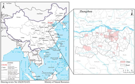
Figure 1. Research location map.

2.1.2. Data Sources and Preprocessing

The analysis employed multi-source datasets, including remote sensing, meteorological, and topographic information (Table 1). Land-cover data were derived from the ESA WorldCover 2020 product (10 m resolution). Meteorological data, including annual mean temperature, precipitation, potential evapotranspiration, and surface solar radiation, were sourced from the China Meteorological Data Sharing Service. Geographic baseline data include slope, aspect, elevation, and soil type. All layers were standardized to a 1 km × 1 km grid in a unified spatial reference using GIS software (ArcMap 10.8), and subsequently aggregated by administrative units (86 urban and 93 rural) for comparison.

Table 1. Summary statistics of data information.

Name	Year	Spatial Resolution	Data Source
Land Use	2020	10 m	ESA WorldCover 2020 (https://viewer.esa-worldcover.org/worldcover, accessed on 12 March 2024)
PM2.5	2020	1 km	CNEMC (China’s National Environmental Monitoring Center), MODIS series products, ERA5 atmospheric reanalysis product, MEIC, SRTM & LandScanTM
DEM	2020	30 m	Geospatial Data Cloud (https://www.gscloud.cn, accessed on 5 April 2024)
Average Temperature in July	2020	1 km	National Earth System Science Data Center (https://www.geodata.cn, accessed on 22 May 2024)
Temperature	2020	1 km	Geographic Data Sharing Infrastructure, global resources data cloud (http://www.gis5g.com, accessed on 18 June 2024)
PET	2020	1 km	National Earth System Science Data Center (https://www.geodata.cn, accessed on 22 May 2024)
Precipitation	2020	1 km	National Earth System Science Data Center (https://www.geodata.cn)
Slope	2020	30 m	National Earth System Science Data Center (https://www.geodata.cn)
Soil	2018	1 km	Chinese soil dataset from the World Soil Database (HWSD) (https://data.tpdc.ac.cn, accessed on 10 July 2024)
Solar Radiation	2020	300 m	National Earth System Science Data Center (https://www.geodata.cn)
NPP	2020	500 m	National Earth System Science Data Center, National Science & Technology Infrastructure of China (http://www.geodata.cn)
NDVI	2020	1 km	MODIS vegetation index dataset (https://lpdaac.usgs.gov, accessed on 10 July 2024)
Nighttime Light	2020	1 km	Plateau Scientific Data Center (https://data.tpdc.ac.cn)

2.2. Methods

This study conducts a multi-faceted assessment of urban–rural differences in ES across four dimensions—potential supply, actual supply, RHN, and effective supply—and then performs spatial optimization (framework in Figure 2).

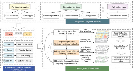
Figure 2. Conceptual framework diagram.

2.2.1. Real Human Needs (RHN)

Based on the established urban–rural spatial division, this study identified urban and rural populations using resident population data. It categorized RHN into three levels: basic needs, desire needs, and spatial needs (Figure 3). Basic needs emphasize essential requirements for survival and development, including a stable food supply and access to clean drinking water. Desire needs to reflect advanced demands driven by socioeconomic development and cultural preferences, including landscape aesthetics and recreational experiences. Spatial needs capture the dependence of population distribution and spatial patterns on residential, working, and recreational spaces [11]. After standardization, all indicators were weighted using the entropy weight method. The results were then aggregated according to the urban–rural population ratio to construct the urban–rural RHN index.

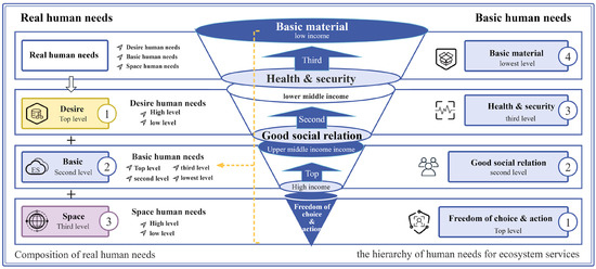
Figure 3. Construction of a framework for Real Human Needs (RHN).

Specifically: (H1) basic needs are primarily driven by material and health pressures related to survival security, and can be characterized by population size and the corresponding welfare level; (H2) desire needs reflect upgraded preferences beyond the survival level, and their spatial distribution is associated with the economic capacity and consumption preferences on the demand side of residents; and (H3) spatial needs capture the crowding pressure in activity and residential spaces and the willingness to obtain spatial resources, jointly influenced by population agglomeration and spatial accessibility. After standardization, indicators at each level are weighted using the entropy weight method and then aggregated according to the urban–rural population ratio to construct the urban–rural RHN index. The composite RHN index is calculated through the following steps.

(1)

Data standardization

Because the indicators have different units, the min–max method is used to standardize them and eliminate the influence of dimensionality. For positive indicators (where larger values indicate higher levels of need), the standardization formula is:

$$Y_{ij}={\displaystyle \frac{X_{ij}-{\mathrm{m}\mathrm{i}\mathrm{n}(X}_j)}{\mathrm{m}\mathrm{a}\mathrm{x}\left(X_j\right)-{\mathrm{m}\mathrm{i}\mathrm{n}(X}_j)}}$$

(1)

For negative indicators, the standardization formula is:

$$Y_{ij}={\displaystyle \frac{{\mathrm{m}\mathrm{i}\mathrm{n}(X}_j)-X_{ij}}{\mathrm{m}\mathrm{a}\mathrm{x}\left(X_j\right)-{\mathrm{m}\mathrm{i}\mathrm{n}(X}_j)}}$$

(2)

where i = 1, …, m denotes the spatial units and j = 1, …, n denotes the indicators. If $\mathrm{m}\mathrm{a}\mathrm{x}\left(X_j\right)={\mathrm{m}\mathrm{i}\mathrm{n}(X}_j)$, then the j-th indicator is constant across all units and is set to $Y_{ij}=0$.

(2)

Entropy-weight method

Indicator weights are determined by the entropy-weight method. Based on the normalized indicators, successively give the proportion $P_{ij}$, the information entropy $e_j$, the differentiation coefficient $g_j$, and the final weight $w_j$.

$$P_{ij}={\displaystyle \frac{Y_{ij}}{{\sum }_{i=1}^m{Y}_{ij}}}$$

(3)

$$e_j=-k\sum _{i=1}^m{P}_{ij}\mathit{ln}{P}_{ij}, k={\displaystyle \frac{1}{\mathit{ln}m}}$$

(4)

$$g_j=1-e_j$$

(5)

$$w_j={\displaystyle \frac{g_j}{{\sum }_{j=1}^n{g}_j}}$$

(6)

(3)

Weighted aggregation and urban–rural weighting

First, the standardized indicator values are weighted and summed according to their entropy weights to obtain the initial RHN index for each basic spatial unit. Then, to reflect the macro-level influence of urban–rural population differences on total demand, the urban and rural areas are treated as two aggregates. The total initial RHN values of urban and rural units are adjusted again using the proportions of permanent urban and rural populations as weights, so that the total RHN of the whole city is consistent with the urban–rural population distribution.

(4)

Basic needs

Based on Maslow’s hierarchy of needs and the Millennium Ecosystem Assessment (MA) definition of human well-being, a four-level framework for human basic needs for ES was established [22]: basic material needs, safety and health, good social relationships, and freedom of choice and action. Subsequently, relative weights were assigned to each level according to World Bank classifications. These weights were then combined with urban–rural population differences to calculate weighted values, resulting in the basic needs level for each region [23].

(5)

Desire needs

Desire needs are represented by regional economic density. In regional economics and ecological economics, economic density (GDP per unit land area) is widely regarded as an effective composite indicator of regional development level, residents’ consumption capacity, and their willingness to pay for higher-order services (such as landscape aesthetics and recreational experiences) [10,24,25]. It indirectly reflects upgraded needs beyond basic survival that are driven by socioeconomic development. In this study, indicators of desire needs are obtained by calculating the total GDP and GDP density for different urban and rural regions.

(6)

Spatial needs

Given human dependence on spaces for work, residence, and leisure, per capita built-up land area and the proportion of public green space are used as indicators of spatial needs [23]. These indicators are intended to measure, at the regional scale, the aggregate demand for the “spatial carriers” of work, residence, and leisure, rather than micro-level individual perceptions. They represent the macro-level manifestation of the expansion and agglomeration of human activities in space and serve as key variables linking population distribution with spatial patterns. They are designed to quantify the intensity of human demand for basic activity spaces such as living, working, and transportation. In macro spatial planning studies, they are regarded as classical indicators of land development intensity and the extent of human spatial occupation. Urban–rural differences in spatial needs are reflected by jointly integrating regional area and population statistics.

2.2.2. Potential Supply

This study focused on six key ES types, selected based on data availability and representativeness. These included provisioning services (food production and water supply), regulating services (carbon sequestration, soil conservation, and gas regulation), and cultural services (recreation and leisure) [22].

(1) Food production: The spatial pattern of potential food production was obtained by redistributing the total statistical grain yield to cropland grid cells according to their NDVI [26].

$$G_{\mathrm{x}}=\left({\displaystyle \frac{{NDVI}_{\mathrm{x}}}{{NDVI}_{\mathrm{s}\mathrm{u}\mathrm{m}}}}\right)\times G_{\mathrm{s}\mathrm{u}\mathrm{m}}$$

(7)

In the formula, $G_{\mathrm{x}}$ represents the food production of the raster $\mathrm{x}$; $G_{\mathrm{s}\mathrm{u}\mathrm{m}}$ is the total food production; ${NDVI}_{\mathrm{x}}$ is the $NDVI$ value of raster $\mathrm{x}$; ${NDVI}_{\mathrm{s}\mathrm{u}\mathrm{m}}$ is the sum of the $NDVI$ values of arable land in the study area.

(2) Water supply: The InVEST water yield module was applied to quantify the potential capacity of water supply services across the study region.

$${\mathrm{W}\mathrm{Y}}_{\mathrm{x}}=\left(1-{\displaystyle \frac{{\mathrm{A}\mathrm{E}\mathrm{T}}_{\mathrm{x}}}{P_{\mathrm{x}}}}\right)P_{\mathrm{x}}$$

(8)

$${\displaystyle \frac{{\mathrm{A}\mathrm{E}\mathrm{T}}_{\mathrm{x}}}{P_{\mathrm{x}}}}=1+{\displaystyle \frac{{\mathrm{P}\mathrm{E}\mathrm{T}}_{\mathrm{x}}}{P_{\mathrm{x}}}}-{\left[1+{\left({\displaystyle \frac{{\mathrm{P}\mathrm{E}\mathrm{T}}_{\mathrm{x}}}{P_{\mathrm{x}}}}\right)}^{w_{\mathrm{x}}}\right]}^{{\displaystyle \frac{1}{w_{\mathrm{x}}}}}$$

(9)

In the formula, ${\mathrm{W}\mathrm{Y}}_{\mathrm{x}}$ is the water yield of cell $\mathrm{x}$ (mm), $P_{\mathrm{x}}$ is the annual precipitation (mm); ${\mathrm{A}\mathrm{E}\mathrm{T}}_{\mathrm{x}}$ is actual evapotranspiration (mm); ${\mathrm{P}\mathrm{E}\mathrm{T}}_{\mathrm{x}}$ is potential evapotranspiration (mm); $w_{\mathrm{x}}$ is an empirical parameter.

(3) Carbon sequestration: Carbon storage was estimated with the InVEST carbon module. Total carbon stock in each cell is calculated as:

$$C_{\mathrm{t}\mathrm{o}\mathrm{t}\mathrm{o}\mathrm{l}}=C_{\mathrm{a}\mathrm{b}\mathrm{o}\mathrm{v}\mathrm{e}}+C_{\mathrm{b}\mathrm{e}\mathrm{l}\mathrm{o}\mathrm{w}}+C_{\mathrm{s}\mathrm{o}\mathrm{i}\mathrm{l}}+C_{\mathrm{d}\mathrm{e}\mathrm{a}\mathrm{d}}$$

(10)

where $C_{\mathrm{t}\mathrm{o}\mathrm{t}\mathrm{o}\mathrm{l}}$ is total carbon sequestration (t); $C_{\mathrm{a}\mathrm{b}\mathrm{o}\mathrm{v}\mathrm{e}}$, $C_{\mathrm{s}\mathrm{o}\mathrm{i}\mathrm{l}}$, $C_{\mathrm{b}\mathrm{e}\mathrm{l}\mathrm{o}\mathrm{w}}$, $C_{\mathrm{d}\mathrm{e}\mathrm{a}\mathrm{d}}$ denote aboveground biomass carbon, belowground biomass carbon, soil carbon, and dead organic matter carbon, respectively.

(4) Soil conservation: Soil conservation quantity is calculated based on the Sediment Delivery Ratio (SDR) module in the In-VEST model. The calculation formula is as follows:

$$SD=RKLS-USLE=R\times K\times LS-R\times K\times LS\times P\times C$$

(11)

where $SD$ is the amount of soil conserved (t hm⁻² a⁻¹); $RKLS$ indicates the potential soil erosion amount under specific climate and terrain conditions (t hm⁻² a⁻¹); $USLE$ is actual soil erosion (t hm⁻² a⁻¹); $R$ is rainfall erosivity (MJ mm hm⁻² h⁻¹ a⁻¹); $K$ is soil erodibility factor (t h MJ⁻¹ mm⁻¹); $LS$ is the slope length factor; $P$ is the soil conservation practice factor; $C$ is the vegetation cover and management factor.

(5) Gas regulation: The purification of PM_2.5 by vegetation was quantified using a dry-deposition approach [27]. The calculation formula is as follows:

$${\mathrm{S}\mathrm{u}\mathrm{p}\mathrm{p}\mathrm{l}\mathrm{y}}_{\mathrm{a}\mathrm{i}\mathrm{r}}=F\times A\times T\times \left(1-R\right)$$

(12)

$$F=V_d\times C\times 3600$$

(13)

In the formula, ${\mathrm{S}\mathrm{u}\mathrm{p}\mathrm{p}\mathrm{l}\mathrm{y}}_{\mathrm{a}\mathrm{i}\mathrm{r}}$ denotes the mass of PM_2.5 removed by surface vegetation on days without rainfall (g); $F$ is the dry deposition flux of PM_2.5 (g/m²·h); $A$ denotes the leaf area (m²); $T$ is the duration (day); $R$ denotes the proportion of PM_2.5 that remains suspended in the atmosphere at a given wind speed. $V_d$ indicates the gravitational deposition rate of PM_2.5 (m/s); $C$ is the concentration of PM_2.5 in the air (g/m³). The wind speed parameters are selected as 0.0015 (m/s) and 4.5 (%) as reference values for $V$ and $R$ [28].

(6) Recreation and leisure: This study examines the differences in recreational and entertainment supply capacity based on the size of green space in each study unit. Green space is categorized into forest and shrubland, while grassland is excluded due to its sparse characteristics [29].

(7) Sources and basis for model parameter settings

The InVEST water production, Carbon, and SDR modules, as well as the Gaussian attenuation model for air regulation, all rely on a set of biophysical and empirical parameters. To ensure reproducibility and regional applicability, the parameter sources are divided into three categories: (1) recommended values from official manuals and published studies: the biophysical table parameters in the InVEST modules (e.g., crop coefficients, root depth and carbon pool densities for different LUCC types) are mainly taken from the recommended values in the InVEST user manual and its associated databases, with priority given to matching typical values reported in studies conducted in Henan Province or Zhengzhou City [30,31,32,33]; (2) parameters such as rainfall erosivity (R factor) and soil erodibility (K factor) are primarily set according to the recommended values of the Chinese Soil Loss Equation (CSLE) and water conservancy census data for Henan Province, with some parameters further validated against regional literature [34]; and (3) empirically derived parameters guided by the literature: the Gaussian attenuation function for air regulation is used to characterize the diffusion and decay of regulating services with distance, and its scale parameter σ is determined with reference to studies of urban ecological regulation at comparable spatial scales [11,25,35], while wind speed and resuspension ratios in the dry deposition model adopt empirical values from existing field-based studies [27,28].

2.2.3. Actual Supply

The actual supply in this study was classified into two categories: commodity-based services and non-commodity-based services [4]. The weights of different ES were determined using the entropy weight method after normalization and directional unification, resulting in a composite index of the actual supply of multiple ES. Among them, commodity-based services (e.g., food production and water supply) can flow across regions through market and transportation systems. In contrast, non-commodity-based services (e.g., carbon sequestration, gas regulation, soil conservation, and Recreation and leisure) primarily benefit humans through ecological diffusion processes or spatial proximity. The specific calculation is as follows:

(1)

Actual supply based on commodity flow

Food production: First, the potential food production supply of each grid cell was calculated using Equation (1). Considering that food is a typical tradable service, its spatial utilization is jointly constrained by transportation impedance and market scale. Therefore, a gravity-based opportunity accessibility model was applied to modify the potential supply. The specific formula is as follows:

$$A_i={\displaystyle \frac{1}{n-1}}{\sum }_{j=1}^n{D}_{ij}$$

(14)

where $A_i$ is accessibility at node $i$; $D_{ij}$ is the minimum impedance between nodes $i$ and $j$; n is the number of nodes. Actual food supply equals potential supply scaled by the accessibility coefficient, reflecting spatial transfer and utilization through transport and markets.

Water supply: First, the potential water supply for each grid cell was calculated using Equations (2) and (3). Then, considering that the spatial allocation of water resources depends on the water supply network and administrative distribution mechanisms, the potential water supply was spatially redistributed according to the water supply data reported in the Zhengzhou Water Resources Bulletin. Finally, the yield was further corrected based on the spatial coverage of the regional water supply system (e.g., reservoir locations and pipeline accessibility) to obtain the actual water resources available for human use.

(2)

Actual supply based on non-commodity flow

Carbon sequestration: As a global public service, carbon sequestration is not affected by direct human accessibility [36]. Considering that carbon sink benefits are primarily realized indirectly through policies (e.g., carbon trading) and regional environmental quality improvements, this study assumes that the actual carbon sequestration equals the potential carbon sequestration, and its “globally shared” nature is discussed in the interpretation of results.

Gas regulation: Gas regulation service represents a typical omnidirectional flow, with its benefits decaying with increasing spatial distance [11,25]. A Gaussian decay function was introduced to describe the spatial diffusion effect of gas regulation services with distance, as follows:

$$Decayed Carbon=Initial Carbon\times \mathrm{e}\mathrm{x}\mathrm{p}\left(-{\displaystyle \frac{{Distance}^2}{{2\sigma }^2}}\right)$$

(15)

In the formula, $Decayed Carbon$ represents the gas regulation amount after decay; $Initial Carbon$ is the initial gas regulation amount; $Distance$ denotes the distance from a point in space to the gas regulation source, indicating the propagation distance of gas regulation. $\sigma$ is the parameter that controls the decay rate.

Soil conservation: The ES flow is in situ; benefits are realized locally [35,37]. Thus, actual Soil conservation equals potential Soil conservation.

Recreation and leisure: A weighted kernel density analysis was applied to estimate the accessibility of recreational green spaces based on the accessibility weights of different regions. Subsequently, the service radiation range of each green space was calculated, and the radiation maps were overlaid with the potential supply map to obtain the actual recreation and leisure service. The kernel density function is expressed as follows:

$$\mathrm{f}\mathrm{n}\left(x\right)={\displaystyle \frac{1}{nh}}{\sum }_{i=1}^{n}k\left({\displaystyle \frac{x-X_i}{h}}\right)$$

(16)

In the formula, $k$ represents the spatial weight; $h$ > 0 is the bandwidth, indicating the degree of smoothing; $x$ is the number of green space patches, and $x-X_i$ denotes the distance from the estimation point to the event $X_i$.

2.2.4. Effective Supply

The effective supply refers to “the amount of ES actually enjoyed by humans”, which depends on the degree of matching between the actual supply and RHN [7,38]. Based on the matching relationship between the total actual supply of six ES types and RHN, a quantitative model of effective supply was constructed.

$$\mathrm{E}\mathrm{f}\mathrm{f}\mathrm{e}\mathrm{c}\mathrm{t}\mathrm{i}\mathrm{v}\mathrm{e} \mathrm{S}\mathrm{u}\mathrm{p}\mathrm{p}\mathrm{l}\mathrm{y}=\left\{\begin{array}{cc}\hfill Actual Supply,& if RHN\ge Actual Supply\hfill \\ \hfill RHN,& if RHN<Actual Supply\hfill \end{array}\right.$$

(17)

2.2.5. Analysis of the Driving Force of the Integrated Actual Supply

This study uses the integrated actual supply as the dependent variable and the driving factors as independent variables, employing R 4.3.3 (in the RStudio environment) for geographic detector analysis [39]. Based on previous research, the selected driving factors include elevation, average annual temperature, annual precipitation, slope, soil type, land use type, net primary productivity (NPP), NDVI, nighttime lights, fraction vegetation cover, leaf area index, and soil erosion factors.

$$q=1-{\displaystyle \frac{{\sum }_{h=1}^L{N}_h{\sigma }_h^2}{N{\sigma }^2}}=1-{\displaystyle \frac{SSW}{SST}}$$

(18)

where $L$ is the number of strata of the explanatory (or dependent) variable, with $N_h$ and $N$ denote the numbers of units in stratum h and in the whole study area, respectively. ${\sigma }_h^2$ and ${\sigma }^2$ are the variances of the Y values for stratum h and the whole area, respectively. $SSW$ and $SST$ are the within-group and total sums of squares.

2.2.6. Spatial Optimization Analysis

This research uses Bayesian principles to calculate the conditional probabilities of each environmental variable concerning the various states of integrated actual supply. Then, key variables are identified by the optimal parameters of the geographic detector model. Finally, the optimization zones are selected based on their state subsets and the distribution of actual supply. The research uses Python (3.12) to build a BBN model. The code implements several key components: setting up model assumptions, processing input data for environmental variables and their conditional probability distributions, learning the dependencies between variables, and conducting model validation. The specific principles of the BBN model are as follows:

Let factor A = {A₁, A₂, ⋯, $A_i$} denote the classified states of a grid-based variable. Let ${SUM}_{Ai}$ be the number of grid cells in state $A_i$ and $SUM$ the total number of cells in the study area. The marginal probability of state $Ai$ is:

$$P_{Ai}={\displaystyle \frac{{SUM}_{A_i}}{SUM}}$$

(19)

Likewise, factor B = {B₁, B₂, ⋯, B_j} represents the states of another variable. Let ${SUM}_{A_i{B}_j}$ be the number of cells where state $A_i$ of $A$ and state $B_j$ of $B$ occur together. The corresponding joint probability is:

$$P\left(A_i{B}_j\right)={\displaystyle \frac{{SUM}_{A_i{B}_j}}{SUM}}$$

(20)

Given that factor $B$ is in state $B_j$, the conditional probability that $A$ takes state $A_i$ is:

$$P\left(A_i|B_j\right)={\displaystyle \frac{P\left(A_i{B}_j\right)}{P\left(B_j\right)}}$$

(21)

In the specific calculations, the actual values of each driving factor are discretized using the ArcGIS 10.2 platform. Each driving factor corresponds to three different states (Table 2). Based on this, Python is used to calculate the integrated actual supply, the number of grids corresponding to each driving factor under different states, and the conditional probabilities of the two factors under different states.

Table 2. Impact Factor and Its Data State Discretization Criteria.

Factors	Name	States 1	Actual Values
Elevation	DEM	1	6–248
		2	248–547
		3	547–1459
Average annual temperature	TEM	1	11.6–14.8
		2	14.8–15.8
		3	15.8–16.6
Annual precipitation	Prec	1	547.8–614.5
		2	614.6–667.1
		3	667.2–874.8
Slope	Slope	1	0–7.4
		2	7.4–19.0
		3	19.0–70.2
Soil types	Soil	1	1. Urban area
		2	2. Rivers; Sandbanks and islands within rivers; Lakes and reservoirs; Tidal soils
		3	3. Coarse-grained soil; Brown soil; Aeolian soil; Yellow loam; New alluvial soil; Chestnut soil
Land use type	LUCC	1	1. Constructed land;
		2	2. Forest vegetation; Shrubland; Cropland; Grassland; Bare/scattered vegetation
		3	3. Water bodies; Wetlands
Net primary productivity	NPP	1	0–154.5
		2	154.6–360.5
		3	360.6–596.9
Normalized difference vegetation index	NDVI	1	0.07–0.51
		2	0.51–0.68
		3	0.68–0.92
Nighttime light	NTL	1	0–1976
		2	1976–4246
		3	4246–6300
Fractional vegetation cover	FAC	1	2981–5,510,391
		2	5,510,391–18,677,633
		3	18,677,633–37,382,701
Leaf area index	LAI	1	0–4
		2	4–9
		3	9–25
Soil erosion factors	K	1	0.03–0.036
		2	0.036–0.041
		3	0.041–0.052
Integrated actual ES supply	IAS	1	0–0.2
		2	0.2–0.3
		3	0.3–1

¹ All driving factors were discretized into three ordinal states based on their spatial distribution using the natural breaks (Jenks) method in ArcGIS 10.2. State 1 = low, State 2 = medium, and State 3 = high.

3. Results

3.1. Contrasting the RHN of Urban and Rural Areas

Urban areas exhibit higher RHN than rural areas, and the shares of basic and desire needs are also higher in urban areas (Figure 4). However, the proportion of units exceeding the citywide mean in RHN, basic needs, and desire needs is lower in urban areas than in rural areas. At the scale of the whole city, RHN presents a clear zonal pattern, with levels tending to be higher in the eastern part of Zhengzhou and gradually weakening toward the west (Figure 4a). Units with high RHN are mainly clustered within the central built-up districts, forming a typical core–periphery structure in which the urban core shows high values surrounded by lower levels in the outer areas. Specifically, urban areas account for 69.70% of total RHN, while rural areas account for 30.30% (Figure 4b). Comparing the distributions (Figure 4c), urban RHN values cluster between 0.2 and 0.4 with a median of 0.3, whereas rural RHN values concentrate around 0.2 with a median of 0.2.

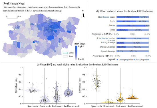
Figure 4. Contrasting RHN in urban and rural areas. (a) Spatial distribution of RHN across urban and rural settings; (b) Urban and rural shares for the three RHN indicators (basic, desire, space); (c) Urban and rural value distributions for the three RHN indicators (basic, desire, space).

3.2. Spatial Contrasts in Potential and Actual Supply Between Urban and Rural Areas

The spatial distributions of potential supply and actual supply for food production, water supply, gas regulation, and recreation and leisure services show significant differences between urban and rural areas (Figure 5). In terms of potential supply, rural areas exhibit higher potential supply for food production, water supply, gas regulation, and recreation and leisure compared to urban areas, overall displaying a decreasing trend from west to east. For actual supply, high-value areas are gradually shifting towards central urban regions. Specifically, the actual supply of food production services in urban areas is higher than in rural areas. In terms of realized services, food production shows higher actual supply levels in urban units than in rural ones. By contrast, rural units provide more water supply than urban units, with the strongest values occurring in the western part of the study area. Areas with high gas-regulation supply are concentrated in the central urban core and in several rural townships to the south, southwest and northwest. Actual recreation and leisure supply is mainly contributed by a limited number of central urban units and by rural areas located in the south, southwest and southeast.

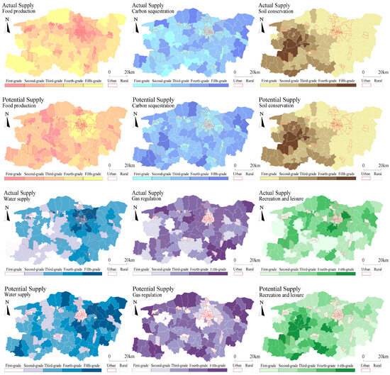
Figure 5. Spatial distribution of potential supply and actual supply in urban and rural areas.

The quantitative differences in both potential supply and actual supply of food production, water supply, gas regulation, and recreation and leisure services are significant between urban and rural areas (Figure 6). The potential and actual supply levels of various ES in rural areas are considerably higher than those in urban areas, indicating a pronounced inequality in ES supply between the two. Rural areas possess stronger ES functions and play a more substantial role in regional ecological support. In contrast, in urban areas, the actual supply of most ES types is higher than their potential supply, reflecting a degree of dependency on rural areas. It underscores the critical role that rural areas play in maintaining ecological balance and providing essential ES.

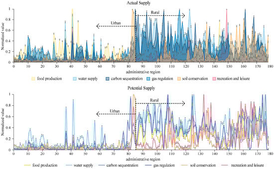
Figure 6. Quantitative comparison of potential supply and actual supply in urban and rural areas. 1–94 represent the urban areas of Zhengzhou, respectively; 95–180 represent rural areas.

High-value clusters of potential supply are formed in rural areas with a relatively intact natural ecological background, whereas actual supply reaches higher levels in some urban areas (Figure 7). This is because urban actual supply is an “available amount” derived from potential supply and further adjusted by factors such as service flows, transport accessibility and population capture capacity; the spatial distribution of urban actual supply therefore does not coincide with the underlying biophysical outputs (potential supply). At the integrated services level, rural areas still maintain the highest total potential supply and actual supply, but because cities possess a stronger capacity to capture services (e.g., food inflows, inter-regional water supply and higher per capita capture efficiency of regulating services), the actual supply of some urban units may be significantly higher than their local potential supply. This pattern reflects a process of redistribution of services rather than an enhancement of the supply capacity of urban ecosystems.

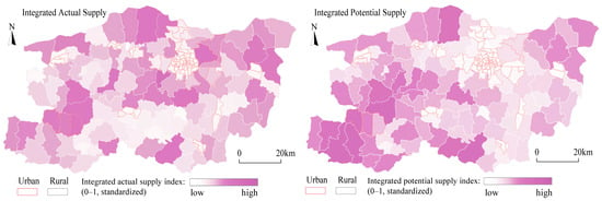
Figure 7. Contrast between actual and potential total supply in urban and rural areas.

3.3. Spatial Distribution and Hierarchy of Effective Supply in Urban and Rural Areas

The spatial distribution of the effective supply levels in Zhengzhou shows significant differences between urban and rural areas (Figure 8). The effective supply values are divided into three levels: high, medium, and low by the natural breaks method. The spatial distribution of effective supply in Zhengzhou indicates a trend of higher values in the central urban area and lower values in surrounding rural regions.

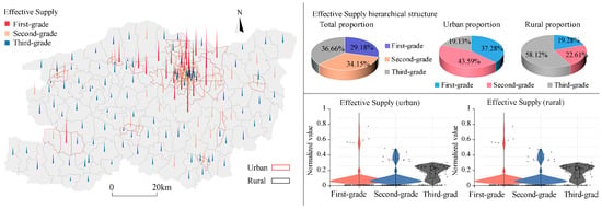
Figure 8. Contrasting effective supply in urban and rural areas.

Concerning the effective supply structure, the highest grade accounts for 29.18% of the total area in Zhengzhou, with the second and third grades accounting for 34.15% and 36.66%, respectively. It suggests that the actual supply of ES in most areas of Zhengzhou is insufficient to meet human needs.

Contrasting urban and rural areas, the proportion of the highest effective supply grade in urban regions is 37.28%, while the second grade accounts for 43.59%. In contrast, the proportions of the highest and second grades in rural areas are 19.28% and 22.61%, respectively. The urban areas thus exhibit a significantly higher proportion of high-grade effective supply compared to rural areas. This disparity suggests that the actual supply of ES in most urban regions is adequate to meet or exceed human demand, contributing to a higher degree of supply-demand matching in urban areas.

3.4. Drivers of Integrated Actual Supply

The geographical detector identified the “dual-dominant” factors controlling the integrated actual supply (Table 3): Fractional Vegetation Cover (FAC, q = 0.676) and annual mean temperature (TEM, q = 0.585). Together, these two factors explain more than 60% of the spatial variation.

Table 3. Results of the Geodetector Model Based on Optimal Parameters.

Factors	q-Value	p-Value	Factors	q-Value	p-Value
FAC	0.676	<0.001	NPP	0.257	<0.001
TEM	0.585	<0.001	K	0.247	<0.001
LAI	0.525	<0.001	LUCC	0.235	<0.001
DEM	0.508	<0.001	NDVI	0.159	<0.001
Slope	0.489	<0.001	Prec	0.155	<0.001
Soil	0.377	<0.001	NTL	0.049	<0.001

3.5. Spatial Pattern Optimization-Urban-Rural Comparison

The results from the conditional probability diagram (Figure 9) indicate that the optimal configurations for the key influencing factors of integrated actual supply, namely FAC and TEM, are FAC = 3 and TEM = 3. Specifically, when vegetation coverage is at the third state (FAC = 3), the probability of achieving optimal integrated actual supply reaches 50.06%. Similarly, when the annual average temperature is at the third state (TEM = 3), the probability of achieving optimal integrated actual supply is 38.76%.

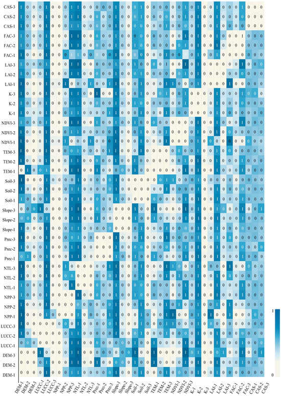
Figure 9. Conditional probability table. Each node is divided into three discrete states. The x-axis lists the states of the conditioning variable B, and the y-axis lists the states of variable A. The value in each cell shows the probability that A takes a given state under a specific state of B(P(A∣B)), with values between 0 and 1. The color scale encodes the magnitude of these conditional probabilities.

Based on the state selection results for FAC = 3 or TEM = 3 (Figure 10), a significant proportion of the area in Zhengzhou achieves optimal FAC. The regions with optimal FAC are primarily located in the western and surrounding rural areas, while urban areas show virtually no regions achieving the optimal state for FAC. Conversely, the areas with optimal TEM are predominantly concentrated in the eastern part of Zhengzhou, with a few small regions in the northeast and southeast also exhibiting the optimal state.

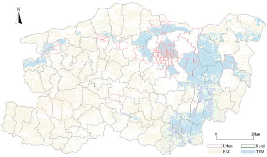
Figure 10. Spatial distribution of critical impact factors.

Supported by ArcGIS 10.2, the distributions of key influencing factors were compared with actual supply to identify areas where both FAC = 3 and TEM = 3 are optimal, but actual supply has not yet reached the optimal level. These areas are defined as the best optimization zones. As shown in Figure 11, the best optimization zones exist in both urban and rural regions; however, overall, they are mainly concentrated in rural areas. Specifically, in urban areas, these zones are primarily scattered in surrounding streets, such as Dongfeng Road, Xiaoyi, Yongan Road, Dufu, and Xinhua Road. In rural areas, the best optimization zones are concentrated in the eastern region, including Guanyinsi Town, Lihe Town, Chengguan Township, Baqian Township, Langchenggang Town, and Sanguanmiao Town.

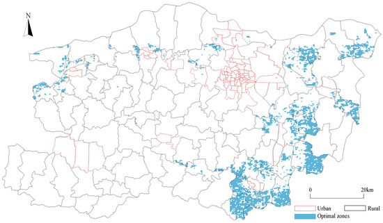
Figure 11. Optimal zones for urban and rural areas.

4. Discussion

4.1. Comprehensive Analysis of Differences in ES Between Urban and Rural Areas

Previous studies comparing urban and rural ES have largely focused on differences in potential supply and potential demand [40]. This study, for the first time, integrates four interconnected dimensions—potential supply, actual supply, RHN, and effective supply—into an urban–rural comparative framework, revealing the complete pathway of supply–demand mismatch. The construction of this framework is a direct response to the limitations of traditional ecosystem services mapping approaches [10,12,25,37]. The results show that RHN in urban areas far exceeds that in rural areas, whereas the potential supply capacity of rural areas is higher than that of urban areas. This confirms the widely observed “urban–rural ecosystem services mismatch” at the global scale [41,42].

Urban and rural areas exhibit systematic differences across three links—“modes of access, directions of flows and efficiency”: urban areas mainly rely on infrastructure-based long-distance imports, whereas rural areas primarily rely on in situ use; urban ES flows are characterized by “external dependence”, while rural ES flows are predominantly “internal self-sufficiency”; the efficiency of ES acquisition in cities is regulated mainly by markets and transport systems, while in rural areas it is jointly constrained by climate and land use [41]. This pattern is consistent with the characteristics of material and energy flows between urban and rural systems described in domestic studies [43,44,45], and is also in line with conclusions from international ES flow typologies [46,47,48].

However, compared with mature regions in Europe and North America [49,50], flows of regulating services in rapidly developing regions such as Zhengzhou are more strongly constrained by green space fragmentation and uneven infrastructure, leading to more pronounced “near-field deficits” in urban areas. This suggests that, in the context of developing countries, institutional arrangements and infrastructure networks may play a significantly stronger role in reshaping ES flow pathways and urban–rural mismatch patterns than in typical cases from Europe and North America. Additionally, policy and regulatory differences play a significant role in ES assessments. For example, rural areas in Henan Province have implemented policies promoting ecological civilization and green agriculture, enhancing ES supply, while urban areas still face insufficient effective supply due to high population density and resource pressures. Multi-dimensional analyses provide a more comprehensive understanding of urban and rural ES supply–demand differences and support differentiated urban and rural development policies.

4.2. Gaps in Effective Supply and Supply–Demand Matching Between Urban and Rural Areas

Previous studies have mostly used the supply–demand ratio to analyze ES supply–demand balance, but such ratios are usually based on static comparisons between potential supply and demand and therefore fail to capture the actual level of satisfaction under constraints of service flows and accessibility [51,52]. This study shifts the focus from a static comparison of “potential supply–demand ratios” to the dynamic relationship between actual supply and RHN. Effective supply is defined as min(AS, RHN), representing the amount of services actually satisfied, and the matching index M = AS/RHN is used to diagnose the spatial distribution of surpluses and deficits. The results indicate that, overall, rural areas still maintain a higher level of effective supply, which implies that their fundamental role as basic supply areas for regional service satisfaction has not been replaced by cities.

On this basis, to further reveal the underlying supply–demand structure and identify optimization targets, the supply–demand matching degree (supply–demand ratio) between actual supply and RHN (Figure 12). shows that approximately 81% of patches with a supply–demand ratio greater than 1 are located in rural areas. These areas exhibit a “supply surplus—demand saturation” pattern and can be identified as ecological sources at the municipal scale and priority output areas for urban–rural ecological compensation. In contrast, about 72% of patches with a supply–demand ratio less than 1 are concentrated in urban areas, forming service-deficit zones characterized by “demand shortfall—insufficient supply”, which need to be alleviated through coordinated regulation that combines local ecological-structure enhancement with the inflow of interregional services [53,54,55]. This configuration is consistent with the common “rural surplus—urban deficit” pattern found in domestic and international urban agglomerations, but is further amplified under conditions of rapid transformation, highlighting the importance of optimizing the spatial coupling between AS and RHN. When surplus in actual supply is brought into balance with RHN, effective ecosystem services in rural areas are significantly improved, and the gap in effective ecosystem services between urban and rural areas is reduced. Adjusting the spatial relationship between actual supply and RHN is therefore crucial for enhancing effective ecosystem services and promoting sustainable development.

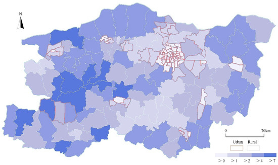
Figure 12. Supply-Demand ratio between actual supply and RHN in urban and rural areas.

4.3. Strategies for Optimizing Urban and Rural ES

Existing research often focuses on optimizing potential supply for a single ES, neglecting multi-service integration and underemphasizing the contribution of actual supply to human well-being, resulting in low optimization efficiency [56,57]. This study, based on multiple ES types, uses composite actual supply as the optimization target, with FAC and TEM as hard constraints, to identify best optimization zones, avoiding blind expansion of green space. Results indicate that the main drivers of composite actual supply are FAC (q = 0.676) and TEM (q = 0.585), with the optimal state combination FAC = 3, TEM = 3. Accordingly, areas satisfying FAC = ∩ TEM = 3 ∩ {integrated actual supply ∈ {1, 2}}—i.e., optimal conditions achieved but output not yet optimal—are defined as best optimization zones.

Differentiated urban–rural strategies are proposed: (1) For urban areas, the focus is on “increasing greening within existing built-up areas + improving network connectivity” to compensate for insufficient FAC. Clustered micro-renovation is implemented in streets with insufficient FAC but favorable TEM (such as Dongfeng Road, Xiaoyi, Yongan Road, Dufu, and Xinhua Road), with the aim of raising the current average level by 10–15%. (2) For rural areas, the focus is on “degradation prevention + production-friendly ecological management” to stabilize FAC and enhance TEM, maintaining and optimizing the existing high coverage and preventing it from degrading below 70%. Ecological ditches, buffer strips, and small wetlands are laid out, together with protective cultivation, in key towns such as Guanyinsi, Lihe, Chengguan, Baqian, Langchenggang, and Sanguanmiao. (3) Regarding corridors and pilot areas, priority is given to restoring continuous corridors along major watercourses and transport greenbelts. Breaks are first eliminated within the best optimization zones to form “point–chain–network” service flow corridors. The Dongfeng Road area and Guanyinsi area can be designated as pilot zones for urban ecological micro-renovation and rural ecological industrialization, respectively, so as to concentrate resources and generate demonstrative effects. Under strict protection of the arable land redline, optimization is advanced in the order of “dual-factor optimal → single-factor optimal → dual-factor non-optimal”, to selectively improve ES supply–demand matching without undermining functional zoning. (4) Achieving the above optimization depends not only on engineering and technical measures but also on strong guidance from public policy. Future efforts could explore the establishment of urban–rural ES compensation mechanisms, enabling cities to provide feedback support for the ecological contributions of rural areas; incorporate ES supply–demand balance indicators into the performance assessment of local governments; and formulate zoned guiding policies (such as urban renewal guidelines and negative lists for rural land use) to ensure that optimization strategies are effectively implemented.

4.4. Limitations and Prospects

This study has several limitations, including uncertainties in basic data (e.g., errors in ESA data and seasonal fluctuations in NDVI) and the incomplete localization of model parameters. Future research could deepen the conclusions by incorporating multi-source validation data, conducting parameter sensitivity analyses, and introducing time-series analysis. Although the quantification of real human needs in this study covers multiple dimensions, the selected indicators (such as using GDP per unit land area to represent desired needs) are still simplified proxies for complex socioeconomic processes. An important direction for improvement will be to introduce more refined proxy variables for demand, for example, by using social media data, questionnaire surveys, or the accessibility of public service facilities to quantify the demand for cultural services.

5. Conclusions

This study takes Zhengzhou City as a case study and establishes a framework of “potential supply–actual supply–RHN–effective supply” to compare urban and rural ES. Subsequently, using the composite actual supply as the optimization target, a geographical detector and a BBN were applied to identify the main driving factors and the best optimization zones, and differentiated optimization strategies were proposed. The main conclusions are as follows:

(1)

Urban RHN markedly exceeds rural and follows an “east-high/west-low, core-high/periphery-low” pattern, with stronger intra-urban inequality. Urban RHN accounts for 69.70% versus 30.30% in rural (a 39.40 percentage-point gap). Urban values cluster at 0.2–0.4 (median 0.3), whereas rural values concentrate at 0.2 (median 0.2). Moreover, the share of units (grid cells) above the citywide mean is lower in urban than in rural areas.

(2)

Zhengzhou exhibits a spatial mismatch—“higher rural potential supply, west > east; actual supply agglomerates toward the urban core”, yielding a net flow from rural to urban. Across multiple ES types, potential supply is overall higher in rural areas with a pronounced western advantage, while bands of high actual supply progressively coalesce in the central city (e.g., food production is higher in the city; Water supply is stronger in rural areas). The southwestern rural zone remains the principal supporting area for composite supply.

(3)

Urban effective supply and supply–demand matching efficiency substantially exceeds rural, while rural areas show a “high-potential/low-conversion” gap. The highest grade of effective supply is 37.28% in urban versus 19.28% in rural. For most ES types, urban areas exhibit actual supply > potential supply. Citywide Grade I/II/III shares are 29.18%/34.15%/36.66%, indicating that over one-third of the area remains supply deficient. Urban areas are characterized by high conversion and high matching; rural shortfalls stem from insufficient conversion efficiency rather than inadequate potential, suggesting policies should target improving the conversion rate per unit of potential supply.

(4)

FAC (q = 0.676) and TEM (q = 0.585) are the key drivers of composite actual supply; identifying priority optimization zones enhances policy precision. Based on BBN optimization (probability of entering the optimal state 50.06% when FAC = 3, 38.76% when TEM = 3), priority optimization zones are concentrated mainly in rural areas, especially eastern rural towns (e.g., Guanyinsi, Lihe), whereas urban optimization zones are primarily located in peripheral subdistricts (e.g., Dongfeng Road, Xiaoyi).

References

- La Notte, A.; Marques, A.; Petracco, M.; Paracchini, M.L.; Zurbaran-Nucci, M.; Grammatikopoulou, I.; Tamborra, M. The assessment of nature-related risks: From ecosystem services vulnerability to economic exposure and financial disclosures. Ecol. Econ. 2025, 235, 108636. [Google Scholar] [CrossRef]
- Fan, Q.; Lu, Q.; Yang, X. Spatiotemporal assessment of recreation ecosystem service flow from green spaces in Zhengzhou’s main urban area. Humanit. Soc. Sci. Commun. 2025, 12, 97. [Google Scholar] [CrossRef]
- Fan, Q.; Wang, Y.; Ping, X. Multiscenario simulations and analyses of urban ecological sources using PLUS and MSPA models: Application in Zhengzhou, China. J. Urban Plan. Dev. 2025, 151, 64. [Google Scholar] [CrossRef]
- Bagstad, K.J.; Johnson, G.W.; Voigt, B.; Villa, F. Spatial dynamics of ecosystem service flows: A comprehensive approach to quantifying actual services. Ecosyst. Serv. 2013, 4, 117–125. [Google Scholar] [CrossRef]
- Bagstad, K.J.; Villa, F.; Batker, D.; Harrison-Cox, J.; Voigt, B.; Johnson, G.W. From theoretical to actual ecosystem services: Mapping beneficiaries and spatial flows in ecosystem service assessments. Ecol. Soc. 2014, 19. [Google Scholar] [CrossRef]
- Fang, Y.X.; Meng, F.H.; Luo, M.; Sa, C.; Bao, Y.H.; Lei, J. Coupling coordination framework for assessing balanced development between potential ecosystem services and human activities. Earth’s Future 2025, 13. [Google Scholar] [CrossRef]
- Burkhard, B.; Kandziora, M.; Hou, Y.; Müller, F. Ecosystem service potentials, flows and demands-concepts for spatial localisation, indication and quantification. Landsc. Online 2014, 34. [Google Scholar] [CrossRef]
- Burkhard, B.; Kroll, F.; Nedkov, S.; Müller, F. Mapping ecosystem service supply, demand and budgets. Ecol. Indic. 2012, 21, 17–29. [Google Scholar] [CrossRef]
- Schröter, M.; Barton, D.N.; Remme, R.P.; Hein, L. Accounting for capacity and flow of ecosystem services: A conceptual model and a case study for Telemark, Norway. Ecol. Indic. 2014, 36, 539–551. [Google Scholar] [CrossRef]
- Villamagna, A.M.; Angermeier, P.L.; Bennett, E.M. Capacity, pressure, demand, and flow: A conceptual framework for analyzing ecosystem service provision and delivery. Ecol. Complex. 2013, 15, 114–121. [Google Scholar] [CrossRef]
- Goldenberg, R.; Kalantari, Z.; Cvetkovic, V.; Mörtberg, U.; Deal, B.; Destouni, G. Distinction, quantification and mapping of potential and realized supply-demand of flow-dependent ecosystem services. Sci. Total Environ. 2017, 593, 599–609. [Google Scholar] [CrossRef] [PubMed]
- Dunford, R.; Harrison, P.; Smith, A.; Dick, J.; Barton, D.N.; Martin-Lopez, B.; Kelemen, E.; Jacobs, S.; Saarikoski, H.; Turkelboom, F.; et al. Integrating methods for ecosystem service assessment: Experiences from real world situations. Ecosyst. Serv. 2018, 29, 499–514. [Google Scholar] [CrossRef]
- Koellner, T.; Schröter, M.; Schulp, C.J.E.; Verburg, P.H. Global flows of ecosystem services. Ecosyst. Serv. 2018, 31, 229–230. [Google Scholar] [CrossRef]
- Mitchell, M.G.E.; Suarez-Castro, A.F.; Martinez-Harms, M.; Maron, M.; McAlpine, C.; Gaston, K.J.; Johansen, K.; Rhodes, J.R. Reframing landscape fragmentation’s effects on ecosystem services. Trends Ecol. Evol. 2015, 30, 190–198. [Google Scholar] [CrossRef]
- Dolan, R.; Bullock, J.M.; Jones, J.P.G.; Athanasiadis, I.N.; Martinez-Lopez, J.; Willcock, S. The flows of nature to people, and of people to nature: Applying movement concepts to ecosystem services. Land 2021, 10, 576. [Google Scholar] [CrossRef]
- Lyu, Y.F.; Wu, C.F. Managing the supply-demand mismatches and potential flows of ecosystem services from the perspective of regional integration: A case study of Hangzhou, China. Sci. Total Environ. 2023, 902, 165918. [Google Scholar] [CrossRef]
- Bruno, E.; Falco, E.; Geneletti, D. Combining demand for ecosystem services with ecosystem conditions of Vacant Lots to support land preservation and restoration decisions. Sustainability 2025, 17, 4686. [Google Scholar] [CrossRef]
- Hsu, W.L.; Zhuang, Z.C.; Li, C.; Zhao, J. Optimization of land use patterns in a Typical Coal resource-based city based on the ecosystem service relationships of ‘food-carbon-recreation’. Land 2025, 14, 661. [Google Scholar] [CrossRef]
- Lapointe, M.; Cumming, G.S.; Gurney, G.G. Comparing ecosystem service preferences between urban and rural dwellers. Bioscience 2019, 69, 108–116. [Google Scholar] [CrossRef]
- Cabañas, R.; Maldonado, A.D.; Morales, M.; Aguilera, P.A.; Salmerón, A. Bayesian networks for causal analysis in socioecological systems. Ecol. Inform. 2025, 89, 103173. [Google Scholar] [CrossRef]
- Yu, Y.Y.; Wang, Y.Q.; Li, J.; Han, L.Q.; Zhang, S.J. Optimizing management of the Qinling-Daba mountain area based on multi-scale ecosystem service supply and demand. Land 2023, 12, 1744. [Google Scholar] [CrossRef]
- Carpenter, S.R.; Mooney, H.A.; Agard, J.; Capistrano, D.; DeFries, R.S.; Díaz, S.; Dietz, T.; Duraiappah, A.K.; Oteng-Yeboah, A.; Pereira, H.M.; et al. Science for managing ecosystem services: Beyond the Millennium Ecosystem Assessment. Proc. Natl. Acad. Sci. USA 2009, 106, 1305–1312. [Google Scholar] [CrossRef]
- Huang, Z.X.; Zhang, Y.L.; Wang, F.F.; Cao, W.Z. Advancing a novel large-scale assessment integrating ecosystem service flows and real human needs: A comparison between China and the United States. J. Clean. Prod. 2021, 314, 14. [Google Scholar] [CrossRef]
- Friesen, J.P.; Kay, A.C.; Eibach, R.P.; Galinsky, A.D. Seeking structure in social organization: Compensatory control and the psychological advantages of hierarchy. J. Pers. Soc. Psychol. 2014, 106, 590–609. [Google Scholar] [CrossRef] [PubMed]
- Fisher, B.; Turner, R.K.; Morling, P. Defining and classifying ecosystem services for decision making. Ecol. Econ. 2009, 68, 643–653. [Google Scholar] [CrossRef]
- Gou, M.; Li, L.; Ouyang, S.; Wang, N.; La, L.; Liu, C.; Xiao, W. Identifying and analyzing ecosystem service bundles and their socioecological drivers in the Three Gorges Reservoir Area. J. Clean. Prod. 2021, 307, 127208. [Google Scholar] [CrossRef]
- Tallis, M.; Taylor, G.; Sinnett, D.; Freer-Smith, P. Estimating the removal of atmospheric particulate pollution by the urban tree canopy of London, under current and future environments. Landsc. Urban Plan. 2011, 103, 129–138. [Google Scholar] [CrossRef]
- Nowak, D.J.; Crane, D.E.; Stevens, J.C. Air pollution removal by urban trees and shrubs in the United States. Urban For. Urban Green. 2006, 4, 115–123. [Google Scholar] [CrossRef]
- Cao, Y.; Cao, Y.; Li, G.; Tian, Y.; Fang, X.; Li, Y.; Tan, Y. Linking ecosystem services trade-offs, bundles and hotspot identification with cropland management in the coastal Hangzhou Bay area of China. Land Use Policy 2020, 97, 104689. [Google Scholar] [CrossRef]
- Li, M.; Zhang, J.C.; Gao, H.S.; Ji, G.X.; Li, G.M.; Li, L.; Li, Q.S. Spatiotemporal variation characteristics of ecosystem carbon storage in Henan Province and future multi-scenario simulation prediction. Land 2024, 13, 185. [Google Scholar] [CrossRef]
- Ma, X.Y.; Liu, S.S.; Guo, L.; Zhang, J.Z.; Feng, C.; Feng, M.Y.; Li, Y.L. Evolution and analysis of water yield under the change of land use and climate change based on the PLUS-InVEST model: A case study of the Yellow River Basin in Henan Province. Water 2024, 16, 2551. [Google Scholar] [CrossRef]
- Zhang, J.C.; Li, L.; Li, Q.S.; Chen, W.Q.; Huang, J.C.; Guo, Y.L.; Ji, G.X. Multiscenario land use change simulation and its impact on ecosystem service function in Henan Province based on FLUS-InVEST model. Ecol. Evol. 2025, 15, ece3.71111. [Google Scholar] [CrossRef] [PubMed]
- Zhou, K.; Wei, X.Y.; Wang, Y.J.; Wang, J.H.; Wang, Z.F.; Zhang, Y.C. Spatiotemporal evolution and prediction of blue-green-grey-space carbon stocks in Henan Province, China. Front. Environ. Sci. 2025, 13, 1545455. [Google Scholar] [CrossRef]
- Guo, Z.Q.; Yan, Z.J.; PaErHaTi, M.; He, R.; Yang, H.; Wang, R.; Ci, H. Assessment of soil erosion and its driving factors in the Huaihe region using the InVEST-SDR model. Geocarto Int. 2023, 38, 2213208. [Google Scholar] [CrossRef]
- Schröter, M.; Koellner, T.; Alkemade, R.; Arnhold, S.; Bagstad, K.J.; Erb, K.-H.; Frank, K.; Kastner, T.; Kissinger, M.; Liu, J.; et al. Interregional flows of ecosystem services: Concepts, typology and four cases. Ecosyst. Serv. 2018, 31, 231–241. [Google Scholar] [CrossRef]
- Li, T.; Li, J.; Wang, Y. Carbon sequestration service flow in the Guanzhong-Tianshui economic region of China: How it flows, what drives it, and where could be optimized? Ecol. Indic. 2019, 96, 548–558. [Google Scholar] [CrossRef]
- Costanza, R. Ecosystem services: Multiple classification systems are needed. Biol. Conserv. 2008, 141, 350–352. [Google Scholar] [CrossRef]
- Burkhard, B.; Crossman, N.; Nedkov, S.; Petz, K.; Alkemade, R. Mapping and modelling ecosystem services for science, policy and practice. Ecosyst. Serv. 2013, 4, 1–3. [Google Scholar] [CrossRef]
- Fan, Q.; Zhang, Y.; Wei, G.; Huang, X. Coupling coordination analysis of urban social vulnerability and human activity intensity. Environ. Res. Commun. 2025, 7, 035009. [Google Scholar] [CrossRef]
- Liu, S.; Shen, P.Y.; Huang, Y.S.; Jiang, L.; Feng, Y.J. Spatial distribution changes in nature-based recreation service supply from 2008 to 2018 in Shanghai, China. Land 2022, 11, 1862. [Google Scholar] [CrossRef]
- Łowicki, D.; Walz, U. Gradient of land cover and ecosystem service supply capacities-a comparison of suburban and rural fringes of towns Dresden (Germany) and Poznan (Poland). Proc. Earth Planet. Sci. 2015, 15, 495–501. [Google Scholar] [CrossRef]
- Lapointe, M.; Gurney, G.G.; Cumming, G.S. Perceived availability and access limitations to ecosystem service well-being benefits increase in urban areas. Ecol. Soc. 2020, 25, 15. [Google Scholar] [CrossRef]
- Chen, D.S.; Li, J.; Yang, X.N.; Zhou, Z.X.; Pan, Y.Q.; Li, M.C. Quantifying water provision service supply, demand and spatial flow for land use optimization: A case study in the YanHe watershed. Ecosyst. Serv. 2020, 43, 101117. [Google Scholar] [CrossRef]
- Chen, H.H.; Li, H.J.; Wang, Y.G.; Cheng, B.Q. A comprehensive assessment approach for water-soil environmental risk during railway construction in ecological fragile region based on AHP and MEA. Sustainability 2020, 12, 7910. [Google Scholar] [CrossRef]
- Li, J.; Zhou, H.W.; Cai, Z.Y. Measuring the smart growth spatial performance in developing city of Northwest China plains area. Geofluids 2021, 2021, 6624478. [Google Scholar] [CrossRef]
- Angela, C.B.; Javier, C.J.; Teresa, G.M.; Marisa, M.H. Hydrological evaluation of a peri-urban stream and its impact on ecosystem services potential. Glob. Ecol. Conserv. 2015, 3, 628–644. [Google Scholar] [CrossRef]
- Balzan, M.V.; Caruana, J.; Zammit, A. Assessing the capacity and flow of ecosystem services in multifunctional landscapes: Evidence of a rural-urban gradient in a Mediterranean small island state. Land Use Policy 2018, 75, 711–725. [Google Scholar] [CrossRef]
- Torres, A.B.; MacMillan, D.C.; Skutsch, M.; Lovett, J.C. Payments for ecosystem services and rural development: Landowners’ preferences and potential participation in western Mexico. Ecosyst. Serv. 2013, 6, 72–81. [Google Scholar] [CrossRef]
- Mandle, L.; Angarita, H.; Moreno, J.; Goldstein, J.A.; Melo, S.F.L.; Echeverri, A.; Rojas, N.; Villalba, F.D. Natural capital accounting reveals ecosystems’ role in water and energy security in Colombia’s Sinú Basin. Commun. Earth Environ. 2025, 6, 309. [Google Scholar] [CrossRef]
- Banerjee, O.; Cicowiez, M.; Torres-Rojo, J.M.; Bagstad, K.J.; Vargas, R.; Edens, B.; Salcone, J.; de Larrea, E.M.B.; Lopez-Conlon, M.; Rodríguez-Ortega, C.; et al. Integrating quantitative macroeconomic and ecosystem service modeling methods to assess conservation programs in Mexico. Environ. Resour. Econ. 2025, 88, 1995–2021. [Google Scholar] [CrossRef]
- Wu, S.Y.; Liu, K.D.; Zhang, W.T.; Dou, Y.H.; Chen, Y.Q.; Zhang, T.P.; Li, D.L. An integrated analysis framework of supply, demand, flow, and use to better understand realized ecosystem services. Ecosyst. Serv. 2024, 69, 101649. [Google Scholar] [CrossRef]
- Zhong, Z.; Fang, X.N.; Zhang, Y.; Shu, X.F.; Guo, D. Mapping ecosystem service supply-demand bundles for an integrated analysis of tradeoffs in an urban agglomeration of China. Land 2022, 11, 1558. [Google Scholar] [CrossRef]
- Danielaini, T.T.; Maheshwari, B.; Hagare, D. Defining rural-urban interfaces for understanding ecohydrological processes in West Java, Indonesia: Part II. Its application to quantify rural-urban interface ecohydrology. Ecohydrol. Hydrobiol. 2018, 18, 37–51. [Google Scholar] [CrossRef]
- Fang, G.J.; Sun, X.; Sun, R.H.; Liu, Q.H.; Tao, Y.; Yang, P.; Tang, H.J. Advancing the optimization of urban-rural ecosystem service supply-demand mismatches and trade-offs. Landsc. Ecol. 2024, 39, 32. [Google Scholar] [CrossRef]
- Sun, X.; Liu, H.; Liao, C.; Nong, H.; Yang, P. Understanding recreational ecosystem service supply-demand mismatch and social groups’ preferences: Implications for urban–rural planning. Landsc. Urban Plan. 2024, 241, 104903. [Google Scholar] [CrossRef]
- Cen, L.Y.; Duan, C.C.; Liu, G.Y.; Chen, B.; Wang, H. Optimized layout of nature-based solutions (NbS) facilities for reducing urban flooding risks and improving ecosystem services. Sustain. Cities Soc. 2025, 130, 106667. [Google Scholar] [CrossRef]
- Mu, Y.L.; Wang, J.; Zhao, C.S.; Li, X.W.; Liu, Y.B.; Lv, J.T. Conservation planning of multiple ecosystem services in the Yangtze River Basin by quantifying trade-offs and synergies. Sustainability 2024, 16, 2511. [Google Scholar] [CrossRef]
Disclaimer/Publisher’s Note: The statements, opinions and data contained in all publications are solely those of the individual author(s) and contributor(s) and not of MDPI and/or the editor(s). MDPI and/or the editor(s) disclaim responsibility for any injury to people or property resulting from any ideas, methods, instructions or products referred to in the content. |
© 2025 by the authors. Licensee MDPI, Basel, Switzerland. This article is an open access article distributed under the terms and conditions of the Creative Commons Attribution (CC BY) license (https://creativecommons.org/licenses/by/4.0/).