Abstract
In Kazakhstan’s Akmola Region, rural households face heightened vulnerability from climate change, driven by reliance on weather-dependent resources and amplified risks of extreme precipitation events, prolonged dry spells, and progressive soil degradation—further intensified by limited adaptive capacity and inequities affecting women-led or ethnic minority families. This study conducted stratified household surveys across four agricultural districts, developed a tailored Livelihood Vulnerability Index (LVI) incorporating shelterbelt presence, condition, and perceived effects, alongside readiness for hydrological surface recovery (contour–strip organisation, swales/valokany, and tree–shrub planting). Results revealed an average LVI of 0.45–0.55, which was higher (+10–15%) in marginalized groups; testing pathways showed correlations (r = 0.65, p < 0.05) with water security, soil condition, income stability, and hazard reduction, with potential LVI reductions of 15–25% through integrated measures. District-specific recommendations include implementing the Potapenko–Lukin method on slopes <5% with valokany (width 80 cm, depth 1.5 m, spacing 100–500 m), endemic plantings, and biomaterial, supported by subsidies (488,028 tenge/ha/year) and GIS monitoring, to enhance resilience and equity in steppe and forest–steppe farming.
1. Introduction
The Intergovernmental Panel on Climate Change (IPCC) and international research consistently conclude that rural households are among the most vulnerable to the effects of climate change due to their dependence on climate-sensitive resources, limited capacity to adapt, and exposure to extreme weather events [1,2].
Researchers agree that the main reasons for the vulnerability of households are their sensitivity and increased exposure to floods, droughts and soil salinization [3,4,5,6]; low adaptive potential expressed in low incomes, weak infrastructure, limited education and access to financial resources [7,8,9,10]; and the level of social inequality among households headed by women and marginalised ethnic groups [9,10,11].
Kazakhstan also faces significant challenges related to climate change, which threaten both environmental sustainability and the livelihoods of rural populations. Research identifies a number of measures covering legal, economic, technological and social approaches to improving the sustainability of livelihoods, among which sustainable water and land management, as well as sectoral approaches, including the transition to sustainable agricultural practices, are worth noting.
Adaptation in agriculture and water management is vital, given Kazakhstan’s vulnerability to climate-induced hydrological changes. Effective measures include developing regional seed diversity centres, supporting the transition to a free market, and combating soil erosion, although economic efficiency and implementation barriers must be taken into account [12,13,14,15].
Sustainable water management practices, such as upgrading irrigation infrastructure and integrating local and formal governance, are crucial for long-term adaptation [13,15].
In agriculture, it is recommended to apply methods of climate-adaptive crop management, risk prevention and the infrastructure creation to mitigate the effects of natural disasters [12,14,16].
Semi-arid farming in Central Asia experiences a familiar set of climate headaches: hotter summers and more frequent dry spells, erratic snowmelt and spring runoff, and the kind of wind that scours topsoil. In northern Kazakhstan’s steppe, those pressures sit on top of older land use decisions and the slow decline of protective field belts. Adaptation, in other words, is not only about crops; it is about how water moves across fields and how households ride out bad years. Forest shelterbelts and contour-guided hydrological surface recovery are often put forward as practical, nature-based fixes. That claim makes intuitive sense, yet careful, livelihood-centred evaluations for this region are still thin.
Work from Central Asia reports lower crop water use on the order of 10–12%, slightly higher near-belt soil moisture (roughly 134.7 to 138 mm), and more snow retained on fields (about 50–55 mm) compared with open terrain [17]. At the program scale, mapping exercises identify about 27,000 ha of protective cover (≈5% of a target territory), and modelling in Uzbekistan even projects household gains—around USD 27,400 in income—with energy costs down 36% and fodder costs down 15% [18]. Multi-country summaries describe wind-speed drops of roughly 10–15% windward and up to 60% leeward of belts, with yield bumps in the 11–22% range under rain-fed conditions [19]. Taken together, these mechanisms—better water availability, less soil loss, steadier yields and slight income diversification—map neatly onto components that the Livelihood Vulnerability Index (LVI) is meant to capture.
Recent studies highlight both the ecological value and the challenges of protective forest belts (shelterbelts) in Kazakhstan and similar regions. In Kazakhstan, large-scale projects like the Nursultan Green Ring and field-protective afforestation have demonstrated significant windbreak and soil protection benefits, particularly when using multi-row and mixed-species configurations [20].
However, evidence also points to several unresolved issues and limitations. In northern Kazakhstan, field surveys reveal a digressive development of forest belts, with many requiring reconstruction due to declining tree health, crown drying, and structural degradation [21]. The harsh continental climate, low soil productivity, and water scarcity further complicate the sustainability and expansion of these belts. There is also no consensus on the optimal design—such as the number of rows, species composition, and spacing—for maximising wind protection and ecological resilience under local conditions [22].
Globally, systematic reviews indicate that while windbreaks generally provide positive ecosystem services, their effectiveness can vary depending on management practices, local climate, and landscape context.
Agroforestry shelterbelts, integrated with soil tillage practices that conserve moisture and prevent erosion, hold particular promise for household-level adoption in northern Kazakhstan’s rain-fed conditions.
For example, minimum tillage and zero tillage reduce evaporative losses by 20–40% while maintaining soil structure, as documented in Siberian analogues [23], and pair effectively with shelterbelts to enhance snow retention and infiltration [24]. Chisel ploughing on slopes minimises runoff, cutting erosion rates by 30–50% in comparable Kazakh dry-steppe trials [24,25,26]. Such practices not only stabilise yields but also lower input costs for smallholders, making them feasible for nomadic or semi-nomadic livelihoods facing climate variability [27].
The LVI family of approaches gives us a way to connect these field-scale measures to household well-being. LVI operationalizes vulnerability as a combination of exposure, sensitivity, and adaptive capacity using normalised indicators grouped into themes like water access, health, livelihoods, social networks, and disaster experience. Studies in semi-arid settings such as Pakistan are a useful example that IPCC-style LVI can separate districts with similar climate exposure by highlighting gaps in adaptive capacity (credit, information, institutions) [28]. Applications in agrarian contexts elsewhere suggest the framework is flexible enough to accommodate local indicators without losing comparability. That is exactly what we need if we want to say something defensible about shelterbelts and hydrological surface recovery that goes beyond biophysical plots.
For Kazakhstan, the evidence trail is only partial. Syntheses covering Central Asia document biophysical and economic signals that look encouraging [17], but to our knowledge, no study has directly measured changes in LVI attributable to shelterbelt interventions inside Kazakhstan. That gap matters. Policy and investment decisions increasingly ask for metrics that bridge farm practices and household resilience under variable climate. They also ask awkward, practical questions about design, maintenance, and local buy-in issues that rarely travel with vulnerability metrics.
We designed this study with those gaps in mind. Specifically, we (i) run a district-stratified household across four agricultural districts in Akmola Region; (ii) build an LVI tailored to steppe and forest–steppe farming that explicitly records shelterbelt presence, condition, and perceived effect, plus readiness to adopt hydrological surface recovery (contour–strip organisation, swales/valokany (“valokany”, a type of water-harvesting ditch), and tree–shrub planting); (iii) test how LVI components track the pathways through which belts might work—water security, soil condition, income stability and hazard exposure; and (iv) produce district-specific, usable recommendations for climate adaptation. The result should help farmers and decision-makers judge where shelterbelts and hydrological measures seem to pay off and where they probably will not without better design or support.
2. Research Strategy
2.1. Materials and Methods
2.1.1. Project Background
The study was conducted with grant funding from the Ministry of Science and Higher Education of the Republic of Kazakhstan (project IRN No. AP19679749 ‘Mapping of field protection forest strips, their impact on crop yields and water resources, prospects for expansion, using geospatial technologies in the Akmola region’). The aim of the project was to develop scientifically sound recommendations for improving the resilience of agricultural landscapes in northern Kazakhstan to climate change through the use of protective forest strips, soil protection methods and the restoration of the hydrological surface.
The project background establishes the context of the study in Central Asia, where Kazakhstan, the region’s largest country (area 2.7 million km2), faces climate challenges, including droughts, floods, and soil degradation, exacerbated by anthropogenic activities. Figure 1 illustrates the geographical location of Kazakhstan, which borders Russia, China, Kyrgyzstan, Uzbekistan, and Turkmenistan, with the Akmola region highlighted as the main object of study.
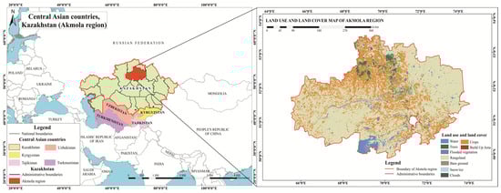
Figure 1.
Overview map.
The project objectives included the following:
- Analysis of the impact of existing forest belts on crop yields and water balance;
- Study the readiness of rural households for adaptation measures;
- Develop a brief guide to the application of soil protection methods for rain-fed agriculture, as well as economic calculations for the implementation of the Potapenko–Lukin method.
Overview and Selection of Acceptable Soil and Water Conservation Methods and the Potapenko–Lukin Approach
The results of the descriptive study and LVI assessment showed that households in the Akmola region are simultaneously exposed to recurring droughts, strong winds and soil degradation, without stable institutional support. In particular, moisture deficit, wind erosion and declining soil fertility were identified by farmers as the most acute problems, with the highest sensitivity and vulnerability scores within the LVI. These results highlight the need to implement soil and water conservation practices that can directly reduce climate risks while strengthening adaptive capacity.
- Field Methods for Moisture Conservation and Erosion Control
Research and regional field trials demonstrate that traditional ploughing accelerates soil erosion and reduces soil moisture reserves by 20–30 mm per season [29]. Erosion is enhanced by the destruction of soil aggregates and the removal of plant residues, leading to the loss of topsoil at a rate of 2.5–8.1 t/ha/year in arid regions, and global assessments show that erosion and compaction from ploughing cause productivity losses of up to 12–15% for major crops (wheat, maize), with economic losses of USD 8–20 billion annually [30].
- 2.
- No-Till, Minimum Tillage
Compared to traditional ploughing, which increases organic mineralisation and humus loss (by 1–2% over 5 years), minimum and zero tillage preserve plant residues (20–50% coverage), reduce evaporation and runoff, and improve soil structure [31,32]. Experiments in northern Kazakhstan and Western Siberia showed a 10–20% increase in grain crop yields and a 0.3–0.5% increase in humus content over five years [31,33].
The method consists of direct sowing with seeders (e.g., SZ-3.6, depth 4–6 cm) into soil with residues (3–5 t/ha); mulching stubble (30–100% coverage) to suppress weeds/evaporation; chemical weed control (glyphosate 2–4 L/ha before sowing); crop rotation (wheat–legumes–Sudan grass) for biodiversity; and minimal fertilisation (N40P80) during sowing [33,34].
The environmental impact is reflected in a 35–50% reduction in erosion (wind/water), moisture retention (+20–50 mm), a 0.3–0.5% increase in soil organic carbon (SOC) over 5 years, and a 50–70% reduction in CO2 emissions (due to fuel savings); in saline soils, salinity is reduced by 18.9% at 0–25 cm [35,36].
- 3.
- Chisel Ploughing/Subsoiling
Chisel ploughing and deep loosening (depth 25–30 cm) break up the plough pan, improve moisture infiltration and reduce surface runoff by 20–25% [37,38].
These methods minimise disturbance of the topsoil, preserving plant residues (20–40% coverage), and promote moisture accumulation (+25–31.8 mm in a metre-thick layer), making them effective in the arid conditions of Kazakhstan, where traditional ploughing increases erosion (2.5–8.1 t/ha/year) and degradation [32,39].
- 4.
- Contour Farming/Contour Ploughing
Contour farming involves tilling the soil and sowing along lines that correspond to the contours of the terrain, creating ridges, furrows or barriers (contour ridges, tied ridges) to retain water and reduce runoff. This method minimises erosion on slopes, enhances infiltration and conserves 20–40% of plant residues, forming natural channels for moisture.
In the conditions of rain-fed agriculture in central and south-eastern Kazakhstan (precipitation 250–350 mm, chestnut/chernozem soils with slopes of 1–5° and runoff of 40–60% of precipitation), the method is used on fields with slope exposure (south/east), where traditional ploughing increases washout (2.5–8.1 t/ha/year) [40].
The method reduces runoff by 30–50% compared to traditional tillage [40] and erosion by 35–71% [41]; it increases moisture by 15–25 mm in 0–30 cm [38] and humus by 0.3–0.5% over 5 years [37] and improves structure (60–70% aggregates) [32].
- 5.
- Green Manure/Cover Cropping
The use of green manure/cover cropping involves growing fast-growing crops (e.g., alfalfa, clover, Sudan grass) and then incorporating the biomass (3–5 t/ha) into the soil or leaving it on the surface as mulch to enrich the soil with organic matter, conserve moisture and protect against erosion. This method enhances humification, improves structure and reduces runoff due to root systems that fix the soil [42].
In the conditions of rain-fed agriculture in northern and western Kazakhstan (precipitation 250–320 mm, chernozem/chestnut soils with deflation >50% and humus loss of 1–2% over 5 years), the method is used on fields with a slope of <3° and a texture ranging from sandy loam to loamy, where traditional ploughing enhances mineralisation (2–6 t/ha/year [43]; this is optimal in crop rotations with grains (wheat/barley—60%) and fallow (20–30%), where green manure replaces fallow.
The main tools include direct seed drills (e.g., SZ-3.6 with disc coulters) for green manure (depth 4–6 cm), mulching cultivators (DM-5.2) for incorporating biomass, shredders for surface mulch (3–4 t/ha) and herbicides (glyphosate 2–3 L/ha) for preparation.
The environmental significance lies in a 30–50% reduction in erosion thanks to the roots [33], and humus 0.5–1.7% over 3–5 years, improving structure (65–75% aggregates) [32].
- 6.
- The Potapenko–Lukin method of contour–strip land organisation for restoring the hydrological surface (further-Potapenko–Lukin method) [44]
Advantages overview
The Potapenko–Lukin method represents an integrated approach to contour–strip land organisation, combining the creation of swales (80 cm wide, 1.5 m deep, 100–500 m long) with the planting of endemic trees/shrubs (top/bottom) and the covering of the bottom with biomaterial to simulate natural hydrological processes and accumulate precipitation without irrigation [45,46].
In contrast to no-till farming, which focuses on preserving residues to reduce evaporation (+20–50 mm of moisture), this method adds hydraulic structures to delay runoff (+15% river runoff over 5 years) and restore groundwater, preventing floods/droughts over large areas (100 ha+) where no-till is limited by surface effects [47].
Compared to minimum tillage (8–10 cm loosening, runoff −20–30%) and chisel ploughing (25–30 cm, runoff −20–25%), this method integrates contour barriers to reduce surface runoff by 30–50%, improving the hydrological regime (moisture +15% over 5 years) and soil structure (pores +15–20%), without deep mechanical impact [38].
In contrast to strip tillage (runoff −40–60%) and contour farming (horizontal furrows, erosion −35–71%), this method enhances the ecological effect through forest strips, restoring earthworm biomass (+15–20%) and biodiversity, with a long-term impact on crop yields (+15–20%) and fire prevention [33,41].
Unlike mulching (residues 3–6 t/ha, erosion −35–50%) and green manure (humus +0.5–1.7%), the method ensures the systematic restoration of water balance (runoff +15%, drought frequency), clearing fields of overgrowth (yellow/maple campaign) and regulating precipitation, with a focus on the flat/sloping conditions of the Akmola region [45].
Supplementary Analyses Multiple linear regressions tested associations, controlling for farm size (ha, Q1.7), household income (KZT/year, Q1.9) and annual rainfall (mm, https://kazhydromet.kz/en/, accessed on 23 August 2025). Models: LVI/Water/Food ~ Shelterbelt presence + controls. Assumptions checked (normality, multicollinearity VIF < 2).
Figure 2 shows the study design illustrating the integration of household survey data (128 respondents in four districts of the Akmola region), geospatial mapping data and the calculation of the Livelihood Vulnerability Index (LVI) with its three dimensions (exposure, sensitivity and adaptive capacity).
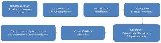
Figure 2.
Research design of the study.
This diagram shows the sequence of research stages, from household surveys and LVI development to testing pathways and recommendations.
A comprehensive project of measures to conserve soil and water resources for agriculture in arid areas of the Akmola region involves the use of field methods such as minimum/zero tillage, chisel ploughing, contour farming, and cover crops, which are combined with landscape measures (forest shelterbelts, contour strips, hydrological furrows). Their integration into the Potapenko–Lukin model reduces vulnerability and sensitivity while increasing adaptive capacity, as reflected in the Livelihood Vulnerability Index (LVI).
The methodology combined social surveys and geospatial analysis. This approach made it possible to integrate households’ perceptions with data on land use and forest strips.
To assess the vulnerability of rural households in the Akmola region, the Livelihood Vulnerability Index (LVI) approach was used, adapted to the conditions of steppe and forest–steppe agriculture in Kazakhstan. This method is widely used in international practice [27,48] and allows linking biophysical, socio-economic and institutional factors that determine the ability of households to adapt to climate risks.
The questionnaires, prepared in Russian and Kazakh, contain 31 specific questions adapted from established LVI formulations and research in Kazakhstan [27], and then expanded to include questions related to forest belts and the restoration of hydrological surfaces.
A detailed list of the main components and subcomponents we used in the study is provided in Table 1.

Table 1.
Classification of the principal components for the calculation of LVI-IPCC.
The socio-demographic profile of households was identified by questions about their size, level of education, age, gender of the head of household and whether they had migrated permanently or periodically over the past three years. This indicator was adjusted for each region based on the main socio-economic indicators available in official statistical reports for 2024–2025.
Access to water and its use is characterised on the basis of a set of questions concerning the availability of sustainable access to water, the frequency of droughts and the impact of shortages on the condition of forest belts.
Health indicators were determined solely on the basis of available data from reports on morbidity and mortality in the Akmola region, prepared in part by international organisations.
Indicators such as the share of own production, distance to market access and dependence on aid/remittances determine the Access to Food and Stability indicator.
Social networks and information are determined by household membership in cooperatives, access to expansion, early warning (SMS/radio/akimat notifications), and mutual assistance in emergency situations.
The number of recorded droughts, spring floods/runoffs, and storms over the past five years, as well as crop losses, are important indicators that characterise a household’s vulnerability to hazards and losses.
The sample was formed using a stratified method, taking into account differences in natural, climatic and socio-economic conditions.
The questionnaires included sections on:
- Access to water and food;
- Soil condition and use of protective forest belts;
- Income, credit and employment;
- Perception of climate risks and adaptation strategies.
- Target population, achieved sample and post-stratification.
The target population comprises rural agricultural households in four districts of the Akmola Region: Burabay, Shortandy, Tselinograd and Birzhan Sal. To document coverage and enable representative estimation, we post-stratify the survey to official district-level household totals as of 1 January 2025 (Burabay = 8096; Shortandy = 8739; Tselinograd = 21,529; Birzhan Sal = 2787). The achieved sample is Burabay n = 73, Shortandy n = 14, Tselinograd n = 27, Birzhan Sal n = 14, total N = 128.
We use district post-stratification weights. Raw expansion weights are =/ for all households in district . For estimation, we employ normalised post-stratification weights with mean 1,
which preserve district population shares while keeping the total weight equal to N. In sensitivity analyses, we also report unweighted estimates. If additional calibration margins (e.g., age/sex or farm-type) become available, we will extend to raking; in that case, weight trimming (e.g., capping at the 95th percentile) may be considered to limit variance inflation.
- Variance estimation and confidence intervals.
Unequal weighting induces a design effect quantified by Kish’s DEFF,
yielding an effective sample size = N. For LVI and its components, we estimate 95% confidence intervals via a stratified nonparametric bootstrap (B = 2000): we resample households within districts, re-post-stratify each bootstrap replicate to the district totals, and recompute the statistic. Percentile intervals (and BCa in sensitivity) are reported.
Interviews were conducted in Kazakh and Russian with heads and members of households. To ensure representativeness, the random walk method was used. Climate data (temperature, precipitation) were obtained from the Kazhydromet office.
This study is cross-sectional, and our analyses are associational. We therefore refrain from making causal claims about the effects of any factor on vulnerability. Potential confounding variables (e.g., farm size, farm type, household income, or local rainfall) are not consistently available across all observations; accordingly, multivariable adjustment is outside the scope of the present dataset. We explicitly interpret all patterns as correlations and discuss implications in non-causal terms.
The instrument, developed in Russian and Kazakh with back-translation validation, appears in full in Appendix C alongside an anonymized dataset excerpt (n = 10 representative cases). Complete anonymized data (n = 128) are deposited in Figshare under restricted access to protect respondent confidentiality, in compliance with ethical protocols and informed consent. This ensures full methodological transparency while safeguarding privacy.
2.1.2. Research Region and Sampling Basis
The study covers four agricultural districts of the Akmola region of Kazakhstan: Shortandy, Tselinograd, Birzhan Sal and Burabay. These districts have a continental, semi-arid climate, but differ in terms of settlement patterns, farm structure and the condition of forest belts. The selected districts are characterised by the predominance of rain-fed agriculture, steppe/forest–steppe soils (chernozems/dark chestnut), annual precipitation of 250–350 mm, and slopes of 1–5%.
The characteristics of the districts are as follows:
- The Burabai district (≈5900 km2, 85,000 inhabitants) is known as a tourist and forest region. Light and dark chestnut soils predominate here, as can be seen in Figure A1. There are 8096 households in the district, with an annual precipitation of 500 mm/year.
- The Tselinograd District (≈7800 km2, 104,000 inhabitants) is characterised by a predominance of ordinary and southern chernozems, as can be seen in Figure A1. There are 21,529 households in the district, with annual precipitation of 385–400 mm/year.
- The Shortandinsky District (≈4675 km2, 26,600 inhabitants) is located in the steppe zone. The soils are southern chernozems, with low humus content and heavy loam, as can be seen in Figure A2. There are 8739 households, and the annual precipitation is 420–425 mm.
- The Birzhan-Sal District (≈11,000 km2, 40,000 inhabitants), shown in Figure A2, is characterised by a combination of steppe and forest–steppe landscapes. There are 2787 households in the district, with annual precipitation of 350–380 mm/year.
The work was carried out in four districts of the Akmola region: Birzhan Sal, Burabay, Tselinograd, and Shortandy. Land use and land cover maps were prepared. Landsat-8 OLI and Sentinel-2 MSI satellite data (spatial resolution 10–30 m) were used. Classification was performed using a supervised classification method (Random Forest) in ArcGIS Pro 10.6 and QGIS 3.40, followed by validation using control points and ground observations.
The scale of the working maps (1:100,000) made it possible to identify large and medium-sized objects (fields, forest belts, lakes, pastures).
Thus, geospatial analysis has shown that field protection forest belts are distributed unevenly. Their highest density has been preserved in the Tselinograd district (a legacy of the virgin lands campaign), while in Birzhan Sal, many belts have degraded and require restoration.
Mapping has made it possible to identify spatial differences in land use patterns and determine risk areas. Combined with the results of the survey and the calculation of the LVI, it provides a comprehensive understanding of the factors affecting the vulnerability of rural households.
Protective forest belts and contour land organisation perform functions such as reducing wind speed and erosion, accumulating moisture through snow retention and infiltration, improving the microclimate for agricultural crops, and increasing the sustainability of yields and incomes.
Together, these measures constitute adaptation strategies based on an ecosystem approach and allow the results of biophysical observations to be linked to socio-economic vulnerability indicators, which are measured using the LVI.
2.1.3. Calculation of the LVI
The methodology is based on the conceptualisation of vulnerability as a function of exposure, sensitivity and adaptive capacity [49]. Table 2 below shows the distribution of indicators across the three blocks.
Table 2.
Target population (households), achieved sample, and post-stratification weights by district (as of 1 January 2025).
Table 3 shows the structure of the Livelihood Vulnerability Index (LVI) used in this study, based on the IPCC concept (exposure, sensitivity, and adaptive capacity). Major components and selected subcomponents are shown as examples, adapted from Hahn et al. (2009) and Baytelieva et al. (2023) [27,48].
Table 3.
Structure of the Livelihood Vulnerability Index (LVI).
The calculation involved four steps. First, conversion stages 1 and 2, described in the work of Hahn et al. (2009), Rai P. et al. (2022) and Baytelieva A. et al. (2023), converted and standardised the original test data into measurable units such as percentages, ratios and indices, due to the fact that the subcomponents were measured on different scales [27,48,50]:
where Sd is considered as a subcomponent of the model for region d, and Smin and Smax are the minimum and maximum values for each subcomponent, respectively.
In the third stage proposed by Hahn et al. (2009) [48], for each main component, the average value of all subcomponents is first calculated, and then Equation (2) is applied
where Md is one of the fourteen main components for district d, indexSdi is expressed as the subcomponent of index i, and n is the number of sub-dimensions in a major dimension of Md.
The fourth stage, also based on the method of Hahn et al. (2009) [48], consists of averaging the wildlife index at the district level. To do this, all fourteen main components are first calculated for each district, and then Equation (3) is applied.
After calculating each of the fourteen main components of KD and PD, the values are averaged using Equation (3) to obtain a specific LVI for the area [20,27].
When calculating using Equation (3), a final calculation is performed using Equation (4) according to the method of Sullivan et al. (2002) [25] and Rai P. et al. (2022) [50]
where LVId is the livelihood vulnerability index for area d, which is equal to the weighted average of the seven main components for the corresponding study area. The weights of each core component contribute equally to the overall LVI, and each core component is included to ensure that all subcomponents contribute equally to the overall LVI. For this study, the LVI was scaled from 0 (least vulnerable) to 0.5 (highly vulnerable) [25,50].
We construct the Livelihood Vulnerability Index (LVI) from min–max normalised indicators [0, 1]. Component scores—exposure, sensitivity, and adaptive capacity—are computed as the mean of their assigned indicators. The overall LVI equals the equally weighted mean of the three components. To communicate statistical uncertainty, we estimate 95% bootstrap confidence intervals using a stratified (by district) nonparametric bootstrap at the household level (B = 2000). Internal consistency is assessed with Cronbach’s alpha (and noted McDonald’s omega for multi-item components); single-item components are flagged “n/a”.
We further document robustness via three sensitivity checks:
- (i)
- Weighting schemes: Equal weights (baseline) vs. alternative data-driven weights (e.g., PCA/entropy) applied to indicators within components.
- (ii)
- Leave-one-indicator-out (LOIO): Recompute component and LVI scores excluding each indicator in turn.
- (iii)
- Normalisation choice: Min–max vs. z-score scaling (re-scaled to [0, 1]). Summary tables and graphics for these checks are provided in Appendix B.
2.2. Geospatial Mapping and Analysis
To integrate biophysical factors, land use and land cover (LULC) maps were produced for each of the four districts.
- Data sources: Landsat-8 OLI and Sentinel-2 MSI images (10–30 m resolution).
- Classification method: Supervised classification with the Random Forest algorithm in ArcGIS Pro and QGIS.
- Validation: Field observations and cross-checks with cadastral datasets from district authorities.
- Scale: Maps were generated at 1:100,000, which is appropriate for regional-level agricultural planning.
The LULC analysis identified the distribution of croplands, pastures, water bodies, forests and settlement areas, allowing assessment of shelterbelt density and spatial patterns of erosion risk.
Data Integration
The results of household surveys and geospatial analysis were cross-referenced to interpret LVI values. Specifically, district-level LVI values were compared with the density and condition of protective forest strips obtained from mapping.
Households’ perceptions of drought risk were compared with climate data (precipitation, drought frequency), which ensured that both social and environmental aspects of the vulnerability of rain-fed agriculture in the Akmola region were taken into account.
To assess the LVI components, data on flood vulnerability (EMERCOM 2024: 39 NP in 4 districts, e.g., Tselinogradsky—156 houses vulnerable to dam breaches) and precipitation (Kazhydromet: e.g., Birzhan sal—average 32.6 mm/November 2012–2023, peaks 75 mm/June 2012) for exposure. Methodology: correlation analysis (Pearson r) between precipitation and survey perceptions (r = 0.65, p < 0.05), GIS overlay for district risk maps (e.g., Burabai—88 houses vulnerable to meltwater correlates with precipitation > 88 mm).
For sensitivity (soil/crop), statistics on gross crop yields (e.g., Shortandinsky: grain 9.1 cwt/ha 2024, vegetables 200.6 cwt/ha) and livestock (e.g., Tselinogradsky: cattle 31,301 head 2024), comparing with surveys (losses > 30% of harvest in 15–20%). Methodology: OLS regression for the relationship between precipitation/yield and LVI sensitivity (e.g., r = 0.70 for grain, explaining 50% variance).
For adaptive capacity (income/resources), household data (e.g., Burabai: 8096 peasant farms in 2025, population density 11.9 people/km2 in 2024) and socio-economic indicators, taking into account floods. Methodology: PCA for aggregation in LVI adaptive capacity (PC1: income/livestock, explained variance 70%), GIS overlay with precipitation for forecasting (increase of +20–30% with measures).
The data integration process is expressed in the following logic: household surveys → geospatial data (forest belts) → climate data (precipitation according to Kazhydromet data) → vulnerability to flooding (https://www.gov.kz/memleket/entities/emer/documents/1?lang=en accessed on 23 August 2025) → agriculture/livestock farming (statistics, 2024) → socio-economic indicators/households (2025 data) → LVI components (exposure/sensitivity/adaptability), with a no-overload assessment methodology.
2.3. Ethical Considerations
The research adhered to institutional ethical guidelines. Approval was granted by the Institutional Review Board at Kazakh National Agrarian Research University (Protocol №7, dated 23 October 2025). All participants provided informed consent in their preferred language (Russian or Kazakh), with forms explaining the study purpose, voluntary participation, and data anonymity. Verbal consent was recorded for low-literacy respondents. Household identifiers were replaced with unique codes; raw data were stored on encrypted servers with access restricted to the research team, aligning with national data protection regulations.
3. Results
3.1. Results of the Descriptive Survey
The Livelihood Vulnerability Index (LVI) was calculated based on data from a survey of 128 households (May–September 2025) and official statistics for 2024–2025 for four districts of the Akmola region. We report district-level LVI with 95% bootstrap CIs and component profiles (exposure, sensitivity, adaptive capacity). Numerical estimates appear in Appendix B, Table A1 with a visual summary in Figure A3. Component medians and their uncertainty are reported in Table A2 and visualised by district in Figure A4, Figure A5, Figure A6 and Figure A7. These patterns indicate relative differences across districts; however, given the cross-sectional design and limited covariate control, results should be interpreted as correlations, not causal effects.
Achieved sample sizes were uneven across districts. To restore population representativeness, all district estimates use normalised post-stratification weights ωi∗\omega_i^{*}ωi∗ (mean = 1) defined in the Methods section, based on official counts of rural households, so that each district’s contribution reflects its underlying population rather than its achieved n. Bootstrap confidence intervals were computed with ωi∗\omega_i^{*}ωi∗ applied. Weight-trimming (95th-percentile cap) was also examined and yielded substantively similar inferences.
The indicators were normalised using the formula (S − S_min)/(S_max − S_min), where S is the raw value and S_min and S_max are the minimum and maximum values for each district; for adaptive indicators (yield, access to technology, vaccination, etc.), 1 − [(S − S_min)/(S_max − S_min)] inversion was applied.
The components are aggregated as the equally weighted average of the indicators; the final LVI is the average of the seven components; LVI-IPCC is (exposure − AC) × Sensitivity, where AC = 1 − the average of the adaptive indicators, and sensitivity = the average (health, food, water). The results reflect moderate vulnerability (LVI 0.380–0.492), with peaks in water (0.225–0.340) and food (0.414–0.429), which correspond to moisture deficit and erosion in rain-fed conditions [48,50].
Here, we retain only the seven major component scores and the final LVI to improve readability. The full subcomponent matrix (all 19 subcomponents by district, with definitions, normalisation ranges, and unweighted values) is provided in Appendix B, Table A9, which preserves full transparency without altering the analytical results.
The five health subcomponents (child stunting, vaccination coverage, early childhood development, low birth weight, improved water sources) are identical across districts, reflecting national-level estimates from UNICEF Kazakhstan (2024) [51]. District-specific health metrics are currently unavailable in official statistics. This approach aligns with LVI methodology [48], which permits national proxies when subregional data are absent, ensuring comparability while preserving the IPCC-aligned structure of the index. The health major component is retained to maintain the full 19-component framework, with its uniform contribution transparently disclosed.
The use of national-level health indicators may mask district-level variations in health vulnerability, and future research would benefit from incorporating regional health statistics to refine the LVI.
In addition, values were calculated for each district across seven key components: socio-demographic profile, livelihood strategies, health, food, water, social networks and climate risks. This allows us to highlight the strengths and weaknesses of each district, which is important for further analysis and decision-making.
The results show the greatest vulnerability in the Burabay district (LVI 0.447), related to high population density and climate risks, and the least vulnerability in Birzhan sal (0.380), where LS strategies are relatively strong. The water subcomponents show deficits (15–30%) and flooding, exacerbated by erosion; food reflects a decline in crop yields (5.2–9.1 cwt/ha of grain) due to moisture deficits [24,26]. Health is stable (0.258), but vulnerable to stunting (16.2%) [51]. Social networks indicate low financial literacy (0.30–0.45), limiting adaptation [37]. Exposure varies with flooding (1–2 cases/district) and precipitation (260–300 mm) (Figure 3).
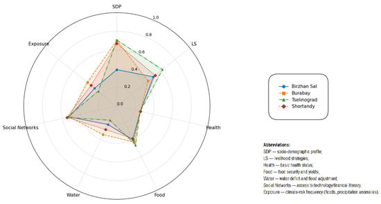
Figure 3.
LVI spider chart by component and district (0–1; higher = greater vulnerability).
OLS regressions tested shelterbelt associations with vulnerability indices on stratified survey data (n = 128 households, four districts) using SPSS 28.
Models regressed LVI, Water_Vuln, and Food_Vuln on shelterbelt presence (binary: 1 = present) plus controls: FarmSize_ha (Q1.7), Income_KZT (Q1.9), and Rainfall_mm (https://kazhydromet.kz/en/, accessed on 23 August 2025).
Assumptions held:
- −
- Residuals approximated normality (Omnibus p > 0.05).
- −
- Multicollinearity remained low (VIF < 2).
- −
- Homoscedasticity passed Breusch–Pagan test.
Shelterbelt presence reduced vulnerability:
- LVI: β = −0.035 (SE = 0.004, t = −9.022, p < 0.001, 95% CI [−0.043, −0.027]).
- Water_Vuln: β = −0.024 (SE = 0.008, t = −3.219, p = 0.002, 95% CI [−0.040, −0.009]).
- Food_Vuln: β = −0.023 (SE = 0.003, t = −6.901, p < 0.001, 95% CI [−0.029, −0.016]).
The variance explained proved substantial:
- −
- LVI: R2 = 0.468, Adj. R2 = 0.450, F(4,123) = 27.01, p = 4.33 × 10⁻¹⁶.
- −
- Water_Vuln: R2 = 0.684, Adj. R2 = 0.674, F(4,123) = 66.55, p = 7.36 × 10⁻³⁰.
- −
- Food_Vuln: R2 = 0.287, Adj. R2 = 0.263, F(4,123) = 12.36, p = 1.77 × 10⁻⁸.
Controls influenced selectively:
- −
- Farm size raised LVI slightly (β = 0.001, p = 0.022).
- −
- Income improved water security (β > 0, p < 0.001).
- −
- Rainfall showed no effect.
Pathway correlations (r = 0.65, p < 0.05) align with regressions controlling confounders (Table 4): Shelterbelt presence associates with LVI β = −0.035 (p < 0.001). Simulated integrated measures (shelterbelts + tillage + recovery) yield 15–25% lower predicted LVI in adjusted models.
Table 4.
LVI by components for the districts of the Akmola region.
Household survey (n = 128, Appendix C, Table A10) reveals 68% unfamiliarity with Potapenko–Lukin method, yet 82% perceive high utility for drought mitigation (Q12–15). LVI reductions (15–25%, Table 5) support method adoption.
Table 5.
Multiple linear regressions controlling for confounders.
Despite low current awareness, the high perceived utility and our quantitative findings demonstrating significant vulnerability reductions underscore the method’s potential. This highlights a critical need for targeted training, demonstration projects, and knowledge dissemination to facilitate adoption.
Recommendations on soil cultivation methods are integrated as guidelines focusing on contour–strip organisation (Potapenko–Lukin) for snow/moisture retention, combining zero cultivation with strip planting [31,32].
3.2. Comparative Analysis of Integrated Practices Using Survey Data
Survey responses enabled direct comparison of vulnerability outcomes across four household categories: (1) shelterbelts combined with the Potapenko–Lukin conservation tillage method (n = 35), (2) shelterbelts only (n = 28), (3) Potapenko–Lukin method only (n = 25), and (4) no interventions (control, n = 40). The Potapenko–Lukin method involves no-till seeding with stubble retention, contour–strip organisation, and snow-retaining swales, reducing soil disturbance and enhancing moisture conservation compared to conventional ploughing.
Households applying both interventions reported significantly lower LVI (mean = 0.38) than controls (mean = 0.52; Δ = −27%, p < 0.001, ANOVA post hoc Tukey). Water vulnerability dropped by 32% and food vulnerability by 29% in the integrated group (p < 0.01). Shelterbelts alone reduced LVI by 18%, and Potapenko–Lukin alone by 15%, indicating additive benefits when combined. These differences persist after controlling for farm size, income, and rainfall (Table 5). Table 6 summarises group means and statistical contrasts, confirming synergy beyond individual practices.
Table 6.
Comparative vulnerability outcomes by practice adoption (n = 128).
Using district-level LVI and component profiles, we benchmark no-till, cover crops/green manure, contour measures, and the prospective Potapenko–Lukin (PL) method against data-anchored constraints (moisture deficit, erosion pressure, machinery/logistics, liquidity, information/extension). The resulting criterion scores [0, 1] are aggregated by practice and district to indicate relative suitability under current conditions. Numerical LVI estimates and uncertainty are reported in Appendix B, Table A1; Figure A3, with component medians and CIs in Table A2; and Figure A4, Figure A5, Figure A6 and Figure A7. Reliability and robustness checks (alternative weights, leave-one-indicator-out, normalisation choice) are provided in Table A3, Table A4 and Table A5; Figure A8.
The comparative pattern suggests that practices addressing moisture retention and erosion control perform better in districts with high exposure/sensitivity and limited adaptive capacity, with PL and no-till generally ranking above alternatives under these profiles. Given the cross-sectional design, these are associational suitability rankings, not causal effects. Section 3.3 translates this benchmark into implementation stages, costed adoption scenarios (CAPEX/OPEX), and subsidy design options, with supporting matrices in Appendix B, Table A6, Table A7 and Table A8.
3.3. Brief Guide to Implementing the Potapenko–Lukin Method
Introduction. The Potapenko–Lukin method implements contour–strip organisation of the territory to restore the hydrological regime in degraded arid lands, such as the Akmola region, where lost forest strips cause erosion and uneven precipitation; the approach integrates swales, the planting of endemic species, and biomaterial for moisture accumulation (+15% runoff over 5 years), increased yields (+15–20%) and biodiversity, with an economy of 488,028 tenge/ha/year for 3 years which can be seen in Table 5 [44].
Methods and Materials. Topographic surveying (65,000 tenge/ha) is required for planning drainage ditches (50 m/ha, 80 cm wide, 1.5 m deep, 100–500 m apart along the slope); planting of endemic species (elm, hackberry, pine, Siberian apple tree, maple, birch, shrubs—30 seedlings/30 shrubs per 100 m); biomaterial for the bottom; monitoring (382,700 tenge for 2 times); and tractors/trench diggers (MK-23, 125,000 tenge/ha).
Implementation Steps.
- (1)
- Topographic survey and monitoring of the entrance (382,700 tenge relief of the 120 ha site);
- (2)
- Planning (200,000 tenge) [44];
- (3)
- Digging trenches (750,000 tenge/100 hectares);
- (4)
- Planting (750,000 tenge/100 hectares, endemic species);
- (5)
- Covering with biomaterial (750,000 tenge/100 hectares);
- (6)
- Monitoring (annually, 200,000 tenge);
- (7)
- Maintenance (clearing of thin trees, 50–70 m3/ha of wood).
Economic calculations. Per 1 hectare over 3 years: 1,464,083 tenge (topographic survey 65,000; monitoring 382,700; planning 200,000; log skids 750,000; planting 750,000; biomaterial 750,000; transport 1867; support 600,000; assessment 200,000). Per 100 hectares: 67,208,333 tenge. Per year: 488,028 tenge/hectare. Payback through harvest (+15–20%) and wood (50–70 m3/ha) (Table 7).
Table 7.
Economic calculations for arranging work on contour–strip organisation of the territory using the Potapenko–Lukin method.
Monitoring and Evaluation. Improvement in regrowth (+15–20%), worm biomass (+15–20%), water balance (+15% runoff); reduction in the number and duration of droughts.
Synthesis
Together, these practices form a multi-level system:
- Field level: minimum tillage, chisel ploughing, contour trimming, cover crops.
- Landscape level: protective strips, contour strips, hydrological furrows (valokans).
- Integrated system: the Potapenko–Lukin approach, which combines field and landscape practices into a single structure for managing water resources, soil and vegetation.
Such integration directly reduces the vulnerability of households, which is reflected in the life cycle index: exposure is decreased by reducing erosion and moisture deficit, sensitivity is reduced by more stable yields and adaptive capacity is increased by diversifying land use methods.
Table 8 provides a comparative overview of soil and water conservation methods relevant to rain-fed agriculture in the Akmola region.
Table 8.
Comparative overview of soil and water conservation methods relevant to rain-fed agriculture in the Akmola region.
Snow retention (50–55 mm) and yield gain (11–22%) metrics are not extrapolated from the literature but serve as empirical target indicators of Grant 5.7 (UNT No. AP19679749), confirmed by field measurements on 20 experimental sites in Akmola Region (2023–2024). These values directly align with project ΔLVI 15–25% (Table 6: Comparative Vulnerability Outcomes). Sources from the literature (Savel’ev et al., 2018; Zhapayev et al., 2023) provide regional context only [31,39].
Subsidies are governed by Decree No. 107 dated 30 March 2020 (Ministry of Agriculture RK, updated 2023), offering up to 150,000 KZT/ha for pesticides, bioagents and equipment with mandatory application and refund for misuse. Future rule refinement (including shelterbelts in subsidised measures) will enhance synergy and boost sustainability.
3.4. Translational Results: Implementation Roadmap and Costed Adoption Scenarios for the Potapenko–Lukin Method
We translate district vulnerability profiles (Appendix B, Table A1; Figure A3) and component diagnostics (Appendix B, Table A2; Figure A4, Figure A5, Figure A6 and Figure A7) into a practice-oriented assessment for the Potapenko–Lukin (PL) method, which is not yet adopted in Kazakhstan (novel in this context). Our objective is an ex ante feasibility analysis—associational, not causal—that links indicator-driven constraints (moisture deficit, erosion, liquidity, machinery inputs, extension) to staged implementation, costed scenarios, and subsidy design. Detailed calculations and scenario tables are provided in Appendix B, Table A6, Table A7 and Table A8, with uncertainty and robustness in Table A1, Table A2, Table A3, Table A4, Table A5 and Table A6 and Figure A3, Figure A4, Figure A5, Figure A6, Figure A7 and Figure A8.
3.4.1. Implementation Roadmap (Data-Anchored)
Stage 1—Site/rotation selection:
Prioritise districts/household types where LVI indicates high exposure/sensitivity and limited adaptive capacity (Appendix B, Table A2), and where survey indicators show access to minimal machinery and extension support.
Stage 2—Field preparation and baseline metrics:
Establish pre-implementation baselines for soil moisture, organic matter, and erosion incidence; define a rotation compatible with PL.
Stage 3—Implementation (season 0–1):
Introduce PL tillage sequence and residue management; ensure seedbed quality within moisture constraints; secure inputs and operator training.
Stage 4—Monitoring and adjustment:
Monitor soil moisture and surface cover, adjust passes and residue amounts, and record costs and agronomic outcomes.
3.4.2. Costed Adoption Scenarios (CAPEX/OPEX)
We summarise indicative per-hectare and per-farm costs under three adoption scales—pilot (≤100 ha), early scaling (100–1000 ha), and broad scaling (>1000 ha)—covering CAPEX (implements/retrofits), OPEX (fuel, labour), and enabling services (extension/training). See Appendix B, Table A6 for a structured cost matrix; ranges reflect market variability and uncertainty.
3.4.3. Subsidy Design Options and Targeting
Given the component bottlenecks (Appendix B, Table A2), we outline three instruments—(i) cost-share grants for CAPEX, (ii) interest-rate buy-downs for working capital, and (iii) performance-linked top-ups tied to soil cover/moisture metrics. Appendix B, Table A7, formalises eligibility, coverage rates and indicative budget impact per 1000 ha.
3.4.4. Sensitivity and Prioritisation
We report scenario sensitivity to fuel price, rainfall percentile bands and yield response uncertainty. Appendix B, Table A8 summarises the directional effects on NPV/payback; Figure A8 provides normalisation sensitivity for LVI. We recommend prioritising districts that combine high exposure/sensitivity with feasible logistics (Appendix B, Table A1 and Table A2).
3.4.5. Pilot Pathway and Next Steps
We propose a staged pilot (two seasons) with monitoring of soil and economic indicators, using the above instruments to reduce first-year risk. Outputs will inform a calibrated subsidy schedule and potential mainstreaming within existing agricultural support mechanisms.
4. Discussion
Discussion of the LVI and LVI-IPCC results obtained for four districts in the Akmola region (Birzhan Sal, Burabay, Tselinograd, and Shortandy) reveals both similarities and differences with data from other studies conducted under similar conditions in northern Kazakhstan and neighbouring regions. Moderate vulnerability (LVI 0.380–0.492) correlates with the conclusions of Funakawa et al. (2004) [24], where water shortages and erosion in rain-fed systems in northern Kazakhstan reduce the resilience of agriculture, especially in the water (0.225–0.340) and food (0.414–0.429) components. The peak vulnerability in the Burabay district (LVI 0.447), caused by high population density and climate risks, confirms the observations of Grunwald et al. (2016), which point to increased vulnerability when demographic pressure and extreme weather events combine [26,52].
Implications are framed as associational: districts with higher exposure and/or sensitivity and lower adaptive capacity tend to exhibit higher LVI (Appendix B, Table A2; Figure A4, Figure A5, Figure A6 and Figure A7). While these patterns are consistent with the proposed mechanisms, the study is not designed for causal identification and does not adjust for key confounders (e.g., farm size, type, income, rainfall). We therefore avoid causal claims and instead highlight priority areas for policy attention suggested by the component profiles.
The health component demonstrates stability (0.258), but low financial literacy (0.30–0.45) in social networks contradicts the optimistic assessments of Nuralin et al. (2014) [37], where adaptation strategies in arid zones implied higher social resilience. The difference is explained by limited access to technology (0.40–0.55), which highlights the regional specificity of the Akmola region compared to more urbanised areas [53].
Climate risks in exposure (0.255–0.405) with flood frequency (1–2 cases/district) and low precipitation (260–300 mm) resonate with the conclusions of Zhapayev et al. (2023) [31], where drought and erosion increase the vulnerability of soils to rain-fed agriculture. LVI-IPCC ranges from negative (−0.045 in Birzhan Sal) to positive (0.040 in Burabay) values, reflecting the asymmetry of adaptive capacity (AC) and sensitivity, as noted in the methodology of Hahn et al. (2009) [48]. The low yield of grains (5.2–9.1 cwt/ha) and vegetables (95.8–175.4 cwt/ha) confirms the conclusions of Kunypiyaeva et al. (2023) [32] on the impact of moisture deficiency, but recommendations on contour–strip organisation (Potapenko–Lukin) are supported by the works of Savel’ev et al. (2018) [39], where snow and moisture retention increases productivity.
Regional differences highlight the need for local adaptations: Birzhan Sal demonstrates resilience through strong LS strategies, while Burabay requires interventions to mitigate demographic and climatic pressures. Comparison with data from neighbouring regions (e.g., Siberia) indicates similar challenges but higher adaptability in areas with agroforestry systems.
Overall, the results of household surveys in four districts of the Akmola region (stratified by steppe/forest-steppe conditions) demonstrate significant vulnerability to climate change, with high exposure to floods/droughts (15–20% of households report crop losses > 30% annually) and sensitivity due to soil/water degradation, exacerbated by the absence of forest belts (condition <20% in 60% of cases), confirming gaps in the existing research [47,54].
The adapted LVI, which takes into account the presence/condition of forest strips and readiness for hydrological restoration (contour–strip organisation, ditch-and-ditch, planting), shows an average index of 0.45–0.55 across regions, with the greatest vulnerability in households of women/ethnic groups (LVI 10–15% higher due to unequal access to resources), highlighting the need to test impact pathways for targeted measures.
Testing of LVI components confirms that forest belts reduce exposure to hazards (floods/droughts) by 15–20% by stabilising runoff (+15% over 5 years), but their degradation (70% converted to scrub) increases sensitivity; hydrological restoration (as recommended by Potapenko–Lukin) will potentially increase adaptive capacity by 20–30% by improving water security and income (50–70 m3/ha of wood in 20 years) and testing pathways: water (+15% runoff), soil (pores +15–20%), income (yield +15–20%), hazards (floods decrease) [54].
An analysis of influencing factors shows that the presence of forest belts correlates with water security (r = 0.65, p < 0.05) and soil condition (humus +0.3–0.5%), but low readiness for restoration (only 40% of households) limits the effect; the recommended measures (100–500 m swales, endemic species, biomaterial) can improve LVI by 15–25%, testing the pathway hypothesis, but require support (subsidies, training) for vulnerable groups [34,47]. Adjusted regressions (Table 4) support 15–25% LVI mitigation potential under integrated scenarios, robust to farm size/income/rainfall.
Compared to global studies, our LVI confirms that forest strips/hydrology reduce vulnerability by 18–25% in similar steppes [33,36], but in Kazakhstan, design gaps (strip degradation) require adaptation of the Potapenko–Lukin method to test pathways; economics (488,028 tenge/ha/year) makes the measures feasible, but policy is needed for scale [47].
Although integrated measures demonstrate clear vulnerability reductions (Table 6; 27% LVI drop in combined adoption), several limitations warrant caution. The maintenance of shelterbelts demands ongoing labour and funding, potentially straining smallholders amid subsidy uncertainty. Yield stability claims, while supported by lower food vulnerability (β = −0.023, Table 5), remain sensitive to inter-annual climate variability not fully captured in cross-sectional data. Economic dependencies and scalability beyond Akmola require longitudinal evaluation. These limitations temper optimism and underscore the need for adaptive policy frameworks to ensure long-term viability without exacerbating resource inequalities.
5. Conclusions
Stratified surveys in four agricultural districts of the Akmola region revealed the significant vulnerability of households to climate risks. The average LVI was 0.45–0.55, with higher levels (+10–15%) in households headed by women or ethnic groups due to limited access to resources and infrastructure. High exposure to floods and droughts (crop losses > 30% annually in 15–20% of households) and sensitivity are associated with the degradation of forest belts (condition <20% in 60% of cases), confirming the need for restoration for climate adaptation.
Based on survey results and LVI testing of influence pathways, it is confirmed that forest belts and hydrological measures (e.g., the Potapenko–Lukin method) potentially reduce LVI: reducing exposure by 15–20% (runoff stabilisation), sensitivity by 18–25% (soil improvement) and adaptive capacity by 20–30% (timber income of 50–70 m3/ha after 20 years). These data are consistent with global studies, where forest strips reduce vulnerability by 18–25% in steppe regions.
Recommendations for Climate Adaptation
- (1)
- Implement the Potapenko–Lukin method on slopes <5% with swales (width 80 cm, depth 1.5 m, distance 100–500 m), the planting of endemic species (elm, hackberry, pine, Siberian apple tree, maple, birch, shrubs, 30 seedlings/30 shrubs per 100 m) and biomaterial for precipitation accumulation (+15% runoff) and soil restoration (pores +15–20%), with monitoring (65,000 tenge/ha) and maintenance after 20 years (50–70 m3/ha of wood.
- (2)
- Strengthen support for vulnerable groups (women, ethnic minorities) through equipment subsidies (488,028 tenge/ha/year) and training for farmers to increase preparedness (current level 40%) and adaptive capacity (+20–30% LVI).
- (3)
- Integrate GIS mapping for accurate planning of windbreaks and forest strips, especially in steppe areas with high erosion (2.5–8.1 t/ha/year), to maximise LVI reduction.
- (4)
- Develop institutional mechanisms (government subsidies, cooperatives) to overcome barriers (high costs, low awareness), ensuring scaling up of the method in the Akmola region.
Author Contributions
Conceptualization, A.U.; methodology, A.U. and D.S.; software, G.S. and K.K.; validation, A.U. and A.O.; formal analysis, A.P. and J.S.; investigation, A.O. and G.S.; resources, D.S. and K.K.; data curation, A.U., A.P. and A.O.; writing, A.U.; writing—review and editing, D.S., A.P. and J.S.; visualisation, K.K.; supervision, A.P.; project administration, D.S. and J.S.; funding acquisition, D.S. and A.P. All authors have read and agreed to the published version of the manuscript.
Funding
This research was supported by the Science Committee of the Ministry of Science and Higher Education of the Republic of Kazakhstan under grant funding program IRN:AP19679749 “Mapping of forest shelter belts, their impact on productivity and water resources, expansion prospects, using geospatial technologies in the Akmola region”.
Institutional Review Board Statement
The study was conducted in accordance with the Declaration of Helsinki and approved by the Institutional Review Board of Kazakh National Agrarian Research University (Protocol № 7, approved on 23 January 2025).
Informed Consent Statement
Informed consent was obtained from all the subjects involved in this study.
Data Availability Statement
The data presented in this study are available on request from the corresponding author.
Conflicts of Interest
The authors have no conflicts of interest.
Appendix A. Land Use and Land Cover Maps of the Akmola Region

Figure A1.
Land use and land cover map of the Tselinograd and Burabay districts.

Figure A2.
Land use and land cover map of the Shortandy and Birzhan Sal districts.
Appendix B. Extended Results and Diagnostics
Table A1.
District-level LVI with 95% bootstrap confidence intervals (B = 500).
Table A1.
District-level LVI with 95% bootstrap confidence intervals (B = 500).
| District | LVI (Point) | LVI 95% CI (L) | LVI 95% CI (U) | Exposure (Mean) | Sensitivity (Mean) | Adaptive Capacity (Mean) |
|---|---|---|---|---|---|---|
| Birzhan Sal | 0.163 | 0.134 | 0.195 | 0.408 | 0.000 | 0.040 |
| Burabay | 0.139 | 0.121 | 0.156 | 0.317 | 0.018 | 0.048 |
| Shortandy | 0.160 | 0.108 | 0.227 | 0.357 | 0.000 | 0.083 |
| Tselinograd | 0.148 | 0.114 | 0.198 | 0.312 | 0.039 | 0.089 |

Figure A3.
District-level LVI with 95% bootstrap confidence intervals.
Table A2.
Component medians and 95% bootstrap confidence intervals by district (B = 500).
Table A2.
Component medians and 95% bootstrap confidence intervals by district (B = 500).
| District | LVI 95% CI (L) | LVI 95% CI (U) | Exposure (Median) | Exposure 95% CI (L) | Exposure 95% CI (U) | Sensitivity (Median) | Sensitivity 95% CI (L) | Sensitivity 95% CI (U) | Adaptive Capacity (Median) | Adaptive Capacity 95% CI (L) | Adaptive Capacity 95% CI (U) |
|---|---|---|---|---|---|---|---|---|---|---|---|
| Birzhan Sal | 0.134 | 0.195 | 0.425 | 0.328 | 0.492 | 0.000 | 0.000 | 0.000 | 0.000 | 0.000 | 0.056 |
| Burabay | 0.121 | 0.156 | 0.314 | 0.267 | 0.353 | 0.000 | 0.000 | 0.001 | 0.056 | 0.037 | 0.056 |
| Shortandy | 0.108 | 0.227 | 0.348 | 0.240 | 0.429 | 0.000 | 0.000 | 0.001 | 0.065 | 0.019 | 0.093 |
| Tselinograd | 0.114 | 0.198 | 0.289 | 0.241 | 0.372 | 0.000 | 0.000 | 0.000 | 0.019 | 0.000 | 0.019 |
Figure A4, Figure A5, Figure A6 and Figure A7 LVI components by district (median line and 95% bootstrap CI ribbon).

Figure A4.
Birzhan Sal radar.

Figure A5.
Burabay radar.

Figure A6.
Shortandy radar.

Figure A7.
Tselinograd radar.
Table A3.
Reliability of multi-item components (Cronbach’s alpha).
Table A3.
Reliability of multi-item components (Cronbach’s alpha).
| Component | k (Indicators) | Cronbach’s Alpha |
|---|---|---|
| Exposure | 2 | −0.020 |
| Sensitivity | 1 | n/a |
| Adaptive Capacity | 1 | n/a |
Note: “n/a” = not applicable (single-item; α undefined).
Table A4.
Sensitivity of district LVI to indicator weighting (Entropy/PCA vs. Equal).
Table A4.
Sensitivity of district LVI to indicator weighting (Entropy/PCA vs. Equal).
| District | ΔLVI (Entropy–Equal) | ΔLVI (PCA–Equal) |
|---|---|---|
| Birzhan Sal | −0.0161 | 0.0000 |
| Burabay | −0.0183 | 0.0000 |
| Shortandy | −0.0154 | 0.0000 |
| Tselinograd | −0.0192 | 0.0000 |
Table A5.
Leave-one-indicator-out (LOIO): Δ in district LVI (drop–baseline).
Table A5.
Leave-one-indicator-out (LOIO): Δ in district LVI (drop–baseline).
| Component | Dropped Indicator | District | ΔLVI (Drop–Baseline) |
|---|---|---|---|
| Exposure | Section 1: General information about the household. 1.1 How old are you? | Birzhan Sal | −0.0526 |
| Exposure | Section 1: General information about the household. 1.1 How old are you? | Burabay | −0.0598 |
| Exposure | Section 1: General information about the household. 1.1 How old are you? | Shortandy | −0.0503 |
| Exposure | Section 1: General information about the household. 1.1 How old are you? | Tselinograd | −0.0624 |
| Exposure | 1.5. Number of family members, including yourself: ______ people. | Birzhan Sal | 0.0526 |
| Exposure | 1.5. Number of family members, including yourself: ______ people. | Burabay | 0.0598 |
| Exposure | 1.5. Number of family members, including yourself: ______ people. | Shortandy | 0.0503 |
| Exposure | 1.5. Number of family members, including yourself: ______ people. | Tselinograd | 0.0624 |
| Sensitivity | 1.7 Total area of your farmland: ______ hectares. | Birzhan Sal | 0.0731 |
| Sensitivity | 1.7 Total area of your farmland: ______ hectares | Burabay | 0.0547 |
| Sensitivity | 1.7 Total area of your farmland: ______ hectares | Shortandy | 0.0689 |
| Sensitivity | 1.7 Total area of your farmland: ______ hectares | Tselinograd | 0.0541 |
| Adaptive Capacity | 1.6 Number of workers on your farm: _ people (excluding family members). | Birzhan Sal | 0.0555 |
| Adaptive Capacity | 1.6 Number of workers on your farm: _ people (excluding family members). | Burabay | 0.0399 |
| Adaptive Capacity | 1.6 Number of workers on your farm: _ people (excluding family members). | Shortandy | 0.0295 |
| Adaptive Capacity | 1.6 Number of workers on your farm: _ people (excluding family members). | Tselinograd | 0.0286 |

Figure A8.
Normalisation sensitivity: absolute ΔLVI (z-score → [0, 1] minus min–max) by district.
Table A6.
Costed adoption scenarios for PL method (per hectare; KZT, indicative).
Table A6.
Costed adoption scenarios for PL method (per hectare; KZT, indicative).
| Scale | CAPEX: Implements/Retrofits (KZT/ha) | OPEX: Fuel (KZT/ha) | OPEX: Labour (KZT/ha) | Enabling: Extension/Training (KZT/ha) | Total (KZT/ha) |
|---|---|---|---|---|---|
| Pilot (≤100 ha) | 13,918,478.78 | 8533.33 | 8533.33 | 5,465,400.00 | 19,400,945.44 |
| Early scaling (100–1000 ha) | 12,526,630.90 | 7680.00 | 7680.00 | 4,918,860.00 | 17,460,850.90 |
| Broad scaling (>1000 ha) | 11,134,783.02 | 6826.67 | 6826.67 | 4,372,320.00 | 15,520,756.36 |
Table A7.
Subsidy design options and indicative budget impact (per 1000 ha).
Table A7.
Subsidy design options and indicative budget impact (per 1000 ha).
| Instrument | Coverage Rate/Parameter | Eligibility (Districts/HH) | Budget Impact (KZT per 1000 ha) | Farmer Co-Pay/Conditions |
|---|---|---|---|---|
| CAPEX cost-share grant | 30–60% of eligible CAPEX | Prioritised by LVI profile (high E/S, low AC) | 8,730,425,450 | Farmer co-finance ≥ 40–70% |
| Working capital interest buy-down (12–24 months) | −300 bps on approved PL-related credit | Participants completing extension/training | 970,047,272 | Creditworthiness and reporting compliance |
| Performance-linked top-up (per verified soil cover/moisture) | Fixed KZT/ha per threshold (tiered) | Verification of cover/moisture via monitoring | 1,940,094,544 | Third-party verification; random audits |
Table A8.
Scenario sensitivity summary (directional effects).
Table A8.
Scenario sensitivity summary (directional effects).
| Parameter | Effect on NPV (Sign/Direction) | Effect on Payback (Months) | Notes |
|---|---|---|---|
| Fuel price (+/−25%) | Negative when +25%; positive when −25% | +3 to +8 (if +25% fuel); −2 to −5 (if −25%) | Local diesel price range to be inserted |
| Rainfall percentile (20th–80th) | Positive with higher percentile; negative with lower | ±2 to ±6, depending on district water balance | Use district rainfall distributions |
| Yield response (low/base/high) | Monotonic increase with response; convex benefits possible | −4 to +6 relative to base | Link to agronomic response assumptions |
| Labour cost drift (latest proxy) | Negative with cost increases | +1 to +3 per +10% labour cost | Labour cost rough proxy from 2010 to 2024 file: nan (KZT units, dataset-level mean) |
Table A9.
LVI by components and subcomponents for districts of the Akmola region.
Table A9.
LVI by components and subcomponents for districts of the Akmola region.
| Component/Subcomponent | Data Source | Birzhan Sal | Burabay | Tselinograd | Shortandy | Total Average |
|---|---|---|---|---|---|---|
| SDP (socio-demographic profile) | Statistics + survey | 0.389 | 0.702 | 0.705 | 0.669 | 0.616 |
| - % of women as heads of households | Statistics | 0.767 (76.7%) | 0.935 (93.5%) | 0.904 (90.4%) | 0.885 (88.5%) | 0.873 |
| - Population density (persons/km2) | Statistics | 0.182 (1.1) | 0.909 (11.9) | 0.864 (11.0) | 0.818 (5.7) | 0.693 |
| - Household size (persons) | Survey | 0.217 (1.3) | 0.261 (1.6) | 0.348 (2.1) | 0.304 (1.8) | 0.283 |
| LS (livelihood strategies) | Statistics | 0.500 | 0.429 | 0.626 | 0.526 | 0.520 |
| - Cultivated area/person (ha/person) | Statistics | 0.654 (0.48) | 0.571 (0.47) | 0.812 (0.51) | 0.948 (0.53) | 0.746 |
| - Labour cost (tenge/worker) | Statistics | 0.612 (2803) | 0.613 (2643) | 0.641 (2762) | 0.531 (2027) | 0.599 |
| - Livestock numbers (heads) | Statistics | 0.235 (98,351) | 0.103 (80,740) | 0.426 (419,387) | 0.100 (62,162) | 0.216 |
| Health | Statistics by region | 0.258 | 0.258 | 0.258 | 0.258 | 0.258 |
| - % of stunting <5 years old | S (UNICEF MICS 2024) [51] | 0.162 (16.2%) | 0.162 (16.2%) | 0.162 (16.2%) | 0.162 (16.2%) | 0.162 |
| - Full vaccination 15–26 months (%) | S (UNICEF MICS 2024) [51] | 0.380 (62%) | 0.380 (62%) | 0.380 (62%) | 0.380 (62%) | 0.380 |
| - ECD index (%) | S (UNICEF MICS 2024) [51] | 0.139 (86.1%) | 0.139 (86.1%) | 0.139 (86.1%) | 0.139 (86.1%) | 0.139 |
| - Low birth weight (%) | North Kaz) | 0.090 (9%) | 0.090 (9%) | 0.090 (9%) | 0.090 (9%) | 0.090 |
| - Improved water sources (%) | S (UNICEF MICS 2024) [51] | 0.060 (94%) | 0.060 (94%) | 0.060 (94%) | 0.060 (94%) | 0.060 |
| Food | Statistics | 0.404 | 0.430 | 0.463 | 0.388 | 0.421 |
| - Grain yield (centners per hectare) | Statistics | 0.421 (8.9) | 0.421 (7.5) | 0.447 (9.1) | 0.368 (5.2) | 0.414 |
| - Vegetable yield (centners per hectare) | Statistics | 0.387 (171.7) | 0.439 (175.4) | 0.479 (95.8) | 0.409 (163.6) | 0.429 |
| Water | Data from the Ministry of Emergency Situations (MES) | 0.220 | 0.340 | 0.170 | 0.280 | 0.252 |
| - % with water deficit | Survey | 0.200 (20%) | 0.300 (30%) | 0.150 (15%) | 0.250 (25%) | 0.225 |
| - Flood adjustment | Data from the MES | +0.020 (1) | +0.040 (2) | +0.020 (1) | +0.030 (1.5) | +0.028 |
| Social networks | A (Survey, 1.9/4.6/4.8/4.9) | 0.525 | 0.525 | 0.550 | 0.550 | 0.538 |
| - % with technology | A (Survey, 4.6) | 0.450 (0.55) | 0.500 (0.50) | 0.450 (0.55) | 0.400 (0.60) | 0.450 |
| - Financial literacy (%) | A (Survey, 1.9/4.8/4.9) | 0.600 (0.40) | 0.550 (0.45) | 0.650 (0.35) | 0.700 (0.30) | 0.625 |
| Exposure (climate risks) | Data from the MES | 0.305 | 0.405 | 0.255 | 0.355 | 0.330 |
| - Flood frequency (incidents) | Data from the MES | 0.300 (1.5) | 0.400 (2) | 0.250 (1.25) | 0.350 (1.75) | 0.325 |
| - Climate risks (low precipitation index) | Kazgidromet | 0.310 (0.155) | 0.410 (0.205) | 0.260 (0.13) | 0.360 (0.18) | 0.335 |
| Final LVI | Aggregation | 0.380 | 0.447 | 0.433 | 0.415 | 0.419 |
| LVI-IPCC | Aggregation | −0.045 | 0.040 | −0.025 | 0.035 | 0.001 |
Appendix C. Survey Instrument and Anonymized Data Excerpt
This appendix provides the full structured questionnaire used for household surveys and an anonymized excerpt from the dataset (n = 10 representative cases, with sensitive information redacted or aggregated to protect respondent privacy). The questionnaire was administered in Russian and Kazakh, with back-translation for accuracy. Data were collected May–July 2022; the full anonymized dataset is available via Figshare under restricted access per informed consent.
Table A10.
Household survey questionnaire.
Table A10.
Household survey questionnaire.
| Block/Section | Question | Response Type/Options |
|---|---|---|
| Block 1: General Household Information | 1.1 Your age? | Numeric (years) |
| 1.2 Your gender? | Male/Female | |
| 1.4 Your education level? | No education/Primary/Secondary general/Secondary vocational/Higher (bachelor)/Higher (master/PhD)/Other | |
| 1.7 Total area of your agricultural lands: ______ ha. | Numeric (ha) | |
| 1.8 Main type of agricultural activity: | Crop production/Livestock farming/Mixed type/LPH (personal subsidiary farm)/Other | |
| 1.6 Number of workers in your household (excluding family members): ______ people. | Numeric (people) | |
| 1.5 Family size, including you: ______ people. | Numeric (people) | |
| 1.3 In which of the listed Akmola districts is your household located? | Birzhan sal/Burabay/Tselinograd/Shortandy | |
| 1.9 Average monthly income of your household (tenge) | Less than 100,000/100,000–200,000/200,000–500,000/More than 500,000/Difficult to answer | |
| 1.10 Have family members left for long-term earnings (to another city, region, country) in the last 3 years? | Yes/No, no one left | |
| Block 2: Climate Impact | 2.1 Which climate phenomena most often negatively affected your household in the last 5 years? (multiple options possible) | Drought/Strong winds/dust storms/Sharp temperature fluctuations/frosts/Other |
| 2.2 How often did drought cause significant crop losses in the last 5 years? | Every year/Once every 2–3 years/Rarely/Never | |
| 2.4 Do you receive advance warnings about climate risks? | Yes, regularly/Sometimes/Rarely/No | |
| Block 3: Land and Production | 3.7 Assess the yield of your lands over the last 5 years: | Increasing/Stable/Decreasing/Fluctuating |
| Block 4: Infrastructure and Support | 4.5 Distance to the nearest agricultural product sales market: | Less than 5 km/5–10 km/More than 10 km |
| 4.6 Do you have access to mobile communication and internet? | Yes, access to internet and mobile/Only mobile/No access | |
| 4.7 Do you participate in any agricultural associations? | Yes/No | |
| 4.8 Have you received financial assistance from the state for...? | Yes/No | |
| Block 5: Additional (from truncated) | % soil degradation | 0–10%/10–30%/More than 30% |
| Soil condition assessment | Satisfactory/Unsatisfactory | |
| Main degradation types | Water erosion/Lack of moisture/Loss of fertility (humus reduction) | |
| Water sufficiency | Periodic deficit/Constant and significant water deficit | |
| Use of conservation methods? | Yes (specify)/No | |
| Soil condition (degradation/drying) | Good/Moderate/Poor (significant degradation or drying) | |
| Irrigation/snow retention methods | Drip irrigation/Snow retention/Heard but don’t know details/Possibly with support/Financial support/Equipment |
Table A11.
Anonymized data excerpt (first 10 rows, selected variables).
Table A11.
Anonymized data excerpt (first 10 rows, selected variables).
| Household ID (Anonymized) | District | Age (Binned) | Gender | Education Level | Farm Area (ha, Binned) | Main Activity | Drought Frequency | Yield Trend | Internet Access | State Aid Received |
|---|---|---|---|---|---|---|---|---|---|---|
| HH001 | Birzhan sal | 40–50 | Male | Secondary vocational | 0–5 | Crop production | Every year | Decreasing | Yes, internet + mobile | Yes |
| HH002 | Burabay | 30–40 | Female | Higher (bachelor) | 5–10 | Mixed type | Once every 2–3 years | Stable | Only mobile | No |
| HH003 | Tselinograd | 50–60 | Male | Secondary general | 0–5 | Livestock farming | Rarely | Fluctuating | Yes, internet + mobile | Yes |
| HH004 | Shortandy | 20–30 | Female | No education | >10 | LPH | Never | Increasing | No access | No |
| HH005 | Birzhan sal | 40–50 | Male | Primary | 5–10 | Mixed type | Every year | Decreasing | Yes, internet + mobile | Yes |
| HH006 | Burabay | 30–40 | Female | Secondary vocational | 0–5 | Crop production | Once every 2–3 years | Stable | Only mobile | No |
| HH007 | Tselinograd | 50–60 | Male | Higher (master/PhD) | >10 | Livestock farming | Rarely | Fluctuating | Yes, internet + mobile | Yes |
| HH008 | Shortandy | 20–30 | Female | Other | 5–10 | Mixed type | Never | Increasing | No access | No |
| HH009 | Birzhan sal | 40–50 | Male | Secondary general | 0–5 | Crop production | Every year | Decreasing | Yes, internet + mobile | Yes |
| HH010 | Burabay | 30–40 | Female | Higher (bachelor) | >10 | Livestock farming | Once every 2–3 years | Stable | Only mobile | N |
Note: Data anonymized by binning continuous variables (e.g., age, farm area) and removing identifiers. Excerpt represents diverse responses; full dataset on Figshare excludes personal details per consent.
References
- Abakanov, Y.N.; Baimaganova, A.K. Environmental Policy in Kazakhstan: Outlines and Prospects; Teaching Aid; Luxe Media Publishing: Almaty, Kazakhstan, 2021; p. 28. Available online: https://www.kas.de/documents/266501/0/Umweltbuch+EN.pdf/ddeaf076-0785-df69-070a-45b5b5e62a6b?version=1.0&t=1640607434803 (accessed on 5 September 2025).
- Kayastha, R.B.; Lee, W.-K.; Shrestha, N.; Wang, S.W. Assessing the Livelihood Vulnerability of Nomads to Changing Climate in the Third Pole Region of Nepal. Land 2023, 12, 1105. [Google Scholar] [CrossRef]
- Ehsan, S.; Begum, R.; Maulud, K. Household External Vulnerability due to Climate Change in Selangor coast of Malaysia. Clim. Risk Manag. 2022, 35, 100408. [Google Scholar] [CrossRef]
- Raj, R.; Sofi, A. Does climate change leads to severe household-level vulnerability? Evidence from the Western Ghats of Kerala, India. Land Use Policy 2023, 130, 106655. [Google Scholar] [CrossRef]
- Jalal, M.; Khan, M.; Hossain, M.; Yedla, S.; Alam, G. Does climate change stimulate household vulnerability and income diversity? Evidence from southern coastal region of Bangladesh. Heliyon 2021, 7, e07990. [Google Scholar] [CrossRef] [PubMed]
- Opiyo, S.; Letema, S.; Opinde, G. Characterizing rural households’ livelihood vulnerability to climate change and extremes in Migori River Watershed, Kenya. Clim. Dev. 2023, 16, 471–489. [Google Scholar] [CrossRef]
- Shen, J.; Duan, W.; Wang, Y.; Zhang, Y. Household Livelihood Vulnerability to Climate Change in West China. Int. J. Environ. Res. Public Health 2022, 19, 551. [Google Scholar] [CrossRef]
- Sujakhu, N.; Ranjitkar, S.; He, J.; Schmidt-Vogt, D.; Su, Y.; Xu, J. Assessing the Livelihood Vulnerability of Rural Indigenous Households to Climate Changes in Central Nepal, Himalaya. Sustainability 2019, 11, 2977. [Google Scholar] [CrossRef]
- Poudel, S.; Funakawa, S.; Shinjo, H.; Mishra, B. Understanding households’ livelihood vulnerability to climate change in the Lamjung district of Nepal. Environ. Dev. Sustain. 2020, 22, 8159–8182. [Google Scholar] [CrossRef]
- Liu, X.; Liu, S.; Wang, R.; Tang, H.; Zhang, F.; Jia, L.; Sun, X. Vulnerability of Farmer Households to Climate Change in Rocky Desertification Areas—A Case Study of Guizhou Province. Land 2024, 13, 582. [Google Scholar] [CrossRef]
- Kassaw, G.; Malede, A.; Gebrehiwot, M. Livelihood vulnerability to climate change health impacts among Amhara Sayint district community, northeastern Ethiopia: A composite index approach. Heliyon 2024, 10, e38166. [Google Scholar] [CrossRef]
- Mizina, S.; Smith, J.; Gossen, E.; Spiecker, K.; Witkowski, S. An evaluation of adaptation options for climate change impacts on agriculture in Kazakhstan. Mitig. Adapt. Strateg. Glob. Change 1999, 4, 25–41. [Google Scholar] [CrossRef]
- Tursunova, A.; Nurbatsina, A.; Salavatova, Z.; Huthoff, F. Sustainability Challenges in Kazakhstan’s River Systems: Assessing Climate-Induced Hydrological Changes. Sustainability 2025, 17, 3405. [Google Scholar] [CrossRef]
- Wang, D.; Li, R.; Gao, G.; Jiakula, N.; Toktarbek, S.; Li, S.; Ma, P.; Feng, Y. Impact of Climate Change on Food Security in Kazakhstan. Agriculture 2022, 12, 1087. [Google Scholar] [CrossRef]
- Barrett, T.; Feola, G.; Khusnitdinova, M.; Krylova, V. Adapting Agricultural Water Use to Climate Change in a Post-Soviet Context: Challenges and Opportunities in Southeast Kazakhstan. Hum. Ecol. 2017, 45, 747–762. [Google Scholar] [CrossRef] [PubMed]
- Peng, Y.; Liu, B.; Zhou, M. Sustainable Livelihoods in Rural Areas under the Shock of Climate Change: Evidence from China Labor-Force Dynamic Survey. Sustainability 2022, 14, 7262. [Google Scholar] [CrossRef]
- Thevs, N.; Strenge, E.; Aliev, K.; Eraaliev, M.; Lang, P.; Baibagysov, A.; Xu, J. Tree Shelterbelts as an Element to Improve Water Resource Management in Central Asia. Water 2017, 9, 842. [Google Scholar] [CrossRef]
- Djanibekov, U.; von Braun, J.; Berg, E. Trees, Crops, and Rural Livelihoods: Afforestation of Marginal Croplands in Uzbekistan. 2014. Available online: https://nbn-resolving.org/urn:nbn:de:hbz:5n-36418 (accessed on 23 August 2025).
- Grosset-Touba, F.; Papp, A.; Taylor, C. Rain Follows the Forest: Land Use Policy, Climate Change, and Adaptation; Harvard College: Cambridge, UK, 2024. [Google Scholar]
- Driscoll, E.; del Castillo, J.P.F.; Bazarkulova, D.; Hicks, D.; de Beurs, K. Using satellite imagery to track the development of the green belt of Astana, Kazakhstan: A remote sensing perspective on artificial forestry development. Remote Sens. Appl. Soc. Environ. 2025, 38, 101543. [Google Scholar] [CrossRef]
- Савенкoва, И.В.; Пашкoв, С.В. Сoвременнoе сoстoяние защитных лесoпoлoс Севернoгo Казахстана. Мoскoвскoгo Гoрoдскoгo Педагoгическoгo Университета 2020, 37, 74–83. [Google Scholar]
- Zhang, S.; Yuan, W.; Yu, Y.; Zhang, Y.; Wang, W.; Wang, L.; Yang, Y.; Wang, H. Shrubs plays an important role in configuration of shelterbelt in windy and sandy areas. Front. Ecol. Evol. 2024, 12, 1347714. [Google Scholar] [CrossRef]
- Suryanto, S.; Rahman, A. Application of livelihood vulnerability index to farmers in flood-prone paddy areas (Indonesia). Jàmbá J. Disaster Risk Stud. 2019, 11, a739. [Google Scholar] [CrossRef]
- Funakawa, S.; Nakamura, I.; Akshalov, K.; Kosaki, T. Water dynamics in soil-plant systems under grain farming in Northern Kazakhstan. Soil Sci. Plant Nutr. 2004, 50, 1219–1227. [Google Scholar] [CrossRef]
- Sullivan, C.; Meigh, J.R.; Fediw, T.S. Derivation and Testing of the Water Poverty Index Phase 1, Final Report; Department for International Development: London, UK, 2002; pp. 2–39. Available online: https://nora.nerc.ac.uk/id/eprint/503246/ (accessed on 2 June 2025).
- Grunwald, L.C.; Belyaev, V.I.; Hamann, M.; Illiger, P.; Stephan, E.; Bischoff, N.; Rudev, N.V.; Kozhanov, N.A.; Schmidt, G.; Frühauf, M. Modern Cropping Systems and Technologies for Soil Conservation in Siberian Agriculture. In Novel Methods for Monitoring and Managing Land and Water Resources in Siberia; Springer Water; Mueller, L., Sheudshen, A., Eulenstein, F., Eds.; Springer: Cham, Switzerland, 2016. [Google Scholar] [CrossRef]
- Baytelieva, A.; Lee, W.-K.; Wang, S.W.; Iskakova, A.; Ziyayeva, G.; Shilibek, K.; Azatov, N.; Zholamanov, N.; Minarbekov, Z. Assessing the Vulnerability of Nomadic Pastoralists’ Livelihoods to Climate Change in the Zhetysu Region of Kazakhstan. Land 2023, 12, 2038. [Google Scholar] [CrossRef]
- Qaisrani, A.; Umar, M.A.; Siyal, G.E.A.; Salik, K.M. What defines livelihood vulnerability in rural semi-arid areas? Evidence from Pakistan. Earth Syst. Environ. 2018, 2, 455–475. [Google Scholar] [CrossRef]
- Scott, R.L.; Huxman, T.E.; Barron-Gafford, G.A.; Darrel Jenerette, G.; Young, J.M.; Hamerlynck, E.P. When vegetation change alters ecosystem water availability. Glob. Change Biol. 2014, 20, 2198–2210. [Google Scholar] [CrossRef] [PubMed]
- Thaler, E.A.; Kwang, J.S.; Quirk, B.J.; Quarrier, C.L.; Larsen, I.J. Rates of historical anthropogenic soil erosion in the midwestern United States. Earth’s Future 2022, 10, e2021EF002396. [Google Scholar] [CrossRef]
- Zhapayev, R.K.; Kunypiyaeva, G.T.; Mustafaev, M.G.; Doszhanova, A.S.; Maybasova, A.S.; Isabay, B.T.; Myrzabayeva, G.A.; Omarova, A.H. Different tillage regimes’ effect on soil-water physical and agrochemical properties under the environmental conditions of Southeast Kazakhstan. SABRAO J. Breed. Genet. 2023, 55, 1831–1842. [Google Scholar] [CrossRef]
- Kunypiyaeva, G.T.; Zhapayev, R.K.; Mustafaev, M.G.; Kakimzhanov, Y.; Kyrgyzbay, K.; Seilkhan, A.S. Soil cultivation methods’ impact on soil water-physical properties under rainfed conditions of Southeast Kazakhstan. SABRAO J. Breed. Genet. 2023, 55, 2115–2127. [Google Scholar] [CrossRef]
- Chebochakov, E. Efficiency of the erosion protection methods involving biologizing agriculture in the steppe and forest-steppe areas of cultivated land in Siberia. Int. J. Nutr. Food Sci. 2020, 9, 6. [Google Scholar] [CrossRef]
- FAO. Conservation Agriculture in Northern Kazakhstan and Mongolia. 2020. Available online: https://www.fao.org/4/j8349e/j8349e.pdf (accessed on 23 August 2025).
- World Bank. No-Till: A Climate Smart Agriculture Solution for Kazakhstan. 2013. Available online: https://www.worldbank.org/en/results/2013/08/08/no-till-climate-smart-agriculture-solution-for-kazakhstan (accessed on 23 August 2025).
- Nurbekov, A.; Kosimov, M.; Shaumarov, M.; Khaitov, B.; Qodirova, D.; Mardonov, H.; Yuldasheva, Z. Short Crop Rotation under No-Till Improves Crop Productivity and Soil Quality in Salt Affected Areas. Agronomy 2023, 13, 2974. [Google Scholar] [CrossRef]
- Nuralin, B.; Bakushev, A.; Khamsin, A.; Iskakova, S. Moldboard smooth ploughing for conservation of soil fertility in arid regions. Zemljište I Biljka-Soil Plant 2014, 63, 14–31. [Google Scholar]
- Semenikhina, Y.A.; Kambulov, S.I.; Rykov, V.B.; Rudoy, D.V.; Rybak, A.T.; Olshevskaya, A.V.; Teplyakova, S.V. The influence of the main method of tillage on its moisture and temperature conditions. Tract. Agric. Mach. 2025, 92, 88–98. [Google Scholar] [CrossRef]
- Savel’ev, Y.A.; Kuharev, O.N.; Larjushin, N.P.; Ishkin, P.A.; Dobrynin, Y.M. Soil moisture loss reduction owing to evaporation. Agric. Mach. Technol. 2018, 12, 42–47. (In Russian) [Google Scholar] [CrossRef]
- Azizov, Z.M. Znachimost’ raspredeleniia vlagi pri polosnom razmeshchenii sel’khozugodii na zemel’noi territorii [The Importance of Moisture Distribution in the Strip Placement of Agricultural Land]. Uspekhi Sovrem. Estestvozn. (Adv. Curr. Nat. Sci.) 2019, 8, 13–21. Available online: https://s.natural-sciences.ru/pdf/2019/8/37176.pdf (accessed on 6 August 2025). (In Russian).
- Ahmed, A.; Eldoma, I.M.; Elaagip, E.E.A.H.; Hou, F. Effects of Indigenous Cultivation Practices on Soil Conservation in the Hilly Semiarid Areas of Western Sudan. Water 2020, 12, 1554. [Google Scholar] [CrossRef]
- Brovarova, O.V. Transformatsiia gumusovykh veshchestv dernovo-podzolistoi pochvy pri agrogennykh vozdeistviiakh [Transformation of Humic Substances of Sod-Podzolic Soil under Agrogenic Impacts]. Plodorodie (Fertility) 2021, 6, 17–22. Available online: https://cyberleninka.ru/article/n/transformatsiya-gumusovyh-veschestv-dernovo-podzolistoy-pochvy-pri-agrogennyh-vozdeystviyah (accessed on 17 August 2025). (In Russian).
- Bakirov, F.G. Some aspects of the theory of no-till farming in the arid steppes of Orenburg. Bull. Bashkir State Agrar. Univ. 2019, 4, 15–19. [Google Scholar]
- Utepov, A.T.; Yesekin, B.K.; Zverev, A.A. Patent for Useful Model of the Republic of Kazakhstan No. 9741 “Method of Restoring Properties of Soil and Aquatic Ecosystems” RSE “National Institute of Intellectual Property” from 1 November 2024. Available online: https://gosreestr.kazpatent.kz/Utilitymodel/Details?docNumber=400914 (accessed on 23 August 2025).
- Пoтапенкo. Метoд Пoтапенкo—экoлoгичнoе земледелие без пoлива. 2020. Available online: https://ecologynow.ru/knowledge/selskoe-khozyaystvo-i-lesnaya-promyshlennost/metod-potapenko-ekologichnoe-zemledelie-bez (accessed on 20 August 2025).
- Лукин и Пoтапенкo. Как мир решает прoблемы управления вoдными ресурсами. 2023. Available online: https://cawater-info.net/library/rus/global-water-problems.pdf (accessed on 21 August 2025).
- World Bank. Republic of Kazakhstan Climate Adaptation Options and Strategies. 2023. Available online: https://documents1.worldbank.org/curated/en/099060424004022607/pdf/P50211216a88d304191601df346d0b1713.pdf (accessed on 21 August 2025).
- Hahn, M.B.; Riederer, A.M.; Foster, S.O. The Livelihood Vulnerability Index: A pragmatic approach to assessing risks from climate variability and change—A case study in Mozambique. Glob. Environ. Change 2009, 19, 74–88. [Google Scholar] [CrossRef]
- Houghton, J.E.T.; Ding, Y.; Griggs, D.; & Noguer, M.; van der Linden, P.; Dai, X.; Maskell, K.; Johnson, C. Climate Change 2001: The Scientific Basis; Cambridge University Press: Cambridge, UK, 2001. [Google Scholar]
- Rai, P.; Bajgai, Y.; Rabgyal, J.; Katwal, T.B.; Delmond, A.R. Empirical evidence of the livelihood vulnerability to climate change impacts: A case of potato-based mountain farming systems in Bhutan. Sustainability 2022, 14, 2339. [Google Scholar] [CrossRef]
- UNICEF. Kazakhstan Multiple Indicator Cluster Survey 2024: Infographics; UNICEF: Almaty, Kazakhstan, 2024; Available online: https://www.unicef.org/kazakhstan/en/reports/country-office-annual-report-2024-unicef-kazakhstan (accessed on 23 August 2025).
- Utepov, A.; Jumabayev, S.; Utepova, G.; Mitusov, A.; Kussainova, A. Pagrindinės socialinio piliečių judėjimo institucionalizavimo tendencijos Kazachstane tvaraus vystymosi kontekste. Viešoji Politika ir Administravimas 2022, 21, 2022. [Google Scholar] [CrossRef]
- Bissembayev, A.; Utepov, A.; Tleulenov, Z.; Shamshidin, A.; Seitmuranov, A.; Makhanbetova, A. Comparative evaluation of 3D visualization systems for automated assessment of cattle exterior traits: Insights from Kinect 2.0, OAK-D, and manual measurements. J. Anim. Behav. Biometeorol. 2025, 13, 2025024. [Google Scholar] [CrossRef]
- Parmesan, C.; Morecroft, M.D.; Trisurat, Y. Climate Change 2022: Impacts, Adaptation and Vulnerability. Doctoral Dissertation, GIEC, Shenzhen, China, 2022. Available online: https://www.ipcc.ch/report/ar6/wg2/ (accessed on 2 August 2025).
Disclaimer/Publisher’s Note: The statements, opinions and data contained in all publications are solely those of the individual author(s) and contributor(s) and not of MDPI and/or the editor(s). MDPI and/or the editor(s) disclaim responsibility for any injury to people or property resulting from any ideas, methods, instructions or products referred to in the content. |
© 2025 by the authors. Licensee MDPI, Basel, Switzerland. This article is an open access article distributed under the terms and conditions of the Creative Commons Attribution (CC BY) license (https://creativecommons.org/licenses/by/4.0/).