Abstract
Microplastic pollution in riverine ecosystems poses critical environmental challenges, yet current modeling approaches inadequately capture the spatial heterogeneity and topological complexity of fluvial systems. This study develops an innovative spatiotemporal graph convolutional network (ST-GCN) framework that integrates hydrological connectivity, flow parameters, and microplastic characteristics for simultaneous migration pathway identification and pollution source tracing. This model constructs multi-scale graph representations encoding system structure and transport dynamics, implements spatial-temporal convolution layers with adaptive attention mechanisms, and employs a backpropagation-based algorithm for inverse source identification. Validation using 18 months of field observations from 45 monitoring nodes across a 127 km river reach demonstrates 87.3% pathway prediction accuracy and 94.3% source localization accuracy (R2 = 0.841, p < 0.001), representing substantial improvements over conventional advection–diffusion models. The framework successfully identified three pollution sources during a real contamination incident within 6 h of detection, enabling rapid regulatory intervention. This research advances environmental modeling by demonstrating that graph neural networks effectively capture transport processes in networked hydrological systems, providing practical tools for watershed management and evidence-based pollution control decision-making.
1. Introduction
Microplastic pollution has emerged as a critical environmental challenge in riverine ecosystems, with particles smaller than 5 mm being transported through complex hydrological networks and accumulating in aquatic environments worldwide [1]. Recent studies have demonstrated that micro- and nanoplastics pose significant ecological risks and biological impacts on aquatic organisms, including oxidative stress, reproductive impairment, and food chain bioaccumulation [2]. The economic burden of microplastic pollution mitigation in aquatic resources is substantial, with global estimates suggesting annual costs exceeding $13 billion for cleanup operations, ecosystem restoration, and fisheries losses [3]. Rivers serve as primary conduits for microplastic transport from terrestrial sources to marine environments, with recent estimates suggesting that riverine systems contribute approximately 80% of oceanic microplastic pollution [4]. Therefore, the identification of migration pathways and accurate tracing of pollution sources remain fundamental prerequisites for developing effective mitigation strategies and pollution control policies.
Current research approaches for microplastic transport modeling predominantly rely on traditional hydrodynamic simulation methods, which incorporate Lagrangian particle tracking and Eulerian advection–diffusion equations [5]. However, these conventional models often inadequately capture the spatial heterogeneity and topological complexity inherent in river networks, leading to substantial uncertainties in pathway prediction [6]. Urban runoff and stormwater systems have been identified as major contributors of contaminated microplastics to aquatic environments, with studies showing that stormwater serves as a key pathway for microplastics entering rivers from diverse urban sources [7]. Recent advances in machine learning have demonstrated promising capabilities in environmental modeling, including convolutional neural networks for pollutant concentration prediction, random forests for source classification, and deep learning models for water quality assessment [8]. However, their application to microplastic transport analysis remains limited by insufficient consideration of the graph-structured nature of river systems [9]. Unlike previous machine learning approaches that treat monitoring data as independent observations, the present study explicitly models river network topology as graph structures, enabling the capture of spatial dependencies along flow pathways. The challenge intensifies when attempting to perform source apportionment, as multiple emission points, diverse polymer types, and varying hydrological conditions create highly complex pollution signatures [10].
Several methodological limitations constrain existing pollution source tracing techniques. Chemical fingerprinting methods, including spectroscopic analysis and polymer identification, can characterize microplastic composition but struggle to establish spatial linkages between sources and downstream contamination sites [11]. Emerging nanoscale detection techniques, such as atomic force microscopy, offer high-resolution characterization of microplastic surface properties but require complex calibration procedures and specialized equipment that limit field applicability [12]. Human biomonitoring approaches provide valuable insights into microplastic exposure pathways but necessitate extensive datasets and face challenges in distinguishing environmental sources [13]. Statistical source apportionment models, such as positive matrix factorization and principal component analysis, demonstrate reduced accuracy when applied to systems with numerous potential sources and overlapping pollution signatures [14]. Furthermore, the lack of integrated frameworks that simultaneously address pathway identification and source tracing restricts a comprehensive understanding of microplastic pollution dynamics in river networks.
Graph convolutional networks (GCNs) provide a powerful computational paradigm for processing data structured as graphs, enabling the extraction of spatial features from topologically connected systems [15]. Unlike conventional neural networks that operate on Euclidean data, GCNs effectively propagate information across network structures while preserving topological relationships, making them particularly suitable for river network analysis [16]. Recent applications of GCNs to environmental monitoring have shown promising results in air quality prediction, traffic-related pollution forecasting, and water quality assessment in urban drainage networks [17]. The application of GCNs to environmental pollution modeling represents an emerging development, with the potential to revolutionize how spatial dependencies and transport mechanisms are represented in complex hydrological systems.
This study develops an innovative GCN-based model for riverine microplastic migration pathway identification and pollution source tracing, addressing critical gaps in current methodologies. The proposed framework integrates river network topology, hydrological parameters, and microplastic characteristics into a unified graph structure, enabling simultaneous analysis of transport dynamics and source attribution [11]. The primary innovations include (1) construction of a multi-scale graph representation that encodes river network structure, flow characteristics, and microplastic properties; (2) development of a spatial-temporal GCN architecture that captures both instantaneous transport processes and long-term accumulation patterns; (3) implementation of an inverse modeling approach for pollution source identification through graph-based feature backpropagation; and (4) integration of uncertainty quantification mechanisms to assess prediction reliability under varying environmental conditions [12]. This research provides both theoretical advances in graph-based environmental modeling and practical tools for watershed management and pollution control decision-making.
2. Theoretical Basis and Related Technologies
2.1. Migration Mechanisms of Riverine Microplastics
Microplastics in riverine systems exhibit distinct occurrence characteristics influenced by particle size, polymer density, and morphological features, with concentrations typically ranging from 0.1 to 50 particles per liter in surface waters [13]. The migration behavior of microplastic particles is governed by advection–diffusion processes, mathematically described by the transport equation:
where represents microplastic concentration, , , denote velocity components in three-dimensional space, , , are diffusion coefficients, and represents source-sink terms.
Table 1 summarizes the physicochemical properties of common microplastic polymers that determine their transport characteristics in aquatic environments. This study focused on conventional petroleum-based polymers (PE, PP, PS, PVC, and PET) that constitute over 90% of microplastics detected in riverine environments. Biodegradable polymers such as polybutylene succinate (PBS) and polylactic acid (PLA) were not included in the current analysis due to their relatively low environmental abundance (<3% of total microplastics in the study area) and distinct degradation kinetics that require separate modeling frameworks.

Table 1.
Physicochemical Properties Parameters of Microplastics.
Settling dynamics play a crucial role in vertical migration, with the terminal settling velocity of spherical microplastic particles calculated using Stokes’ law [14]:
where is gravitational acceleration, and represent particle and water density, respectively, is particle diameter, and denotes dynamic viscosity.
Resuspension occurs when bed shear stress exceeds critical thresholds, quantified by the Shields parameter [15]:
where represents bed shear stress. Hydrodynamic conditions, including flow velocity, turbulence intensity, and discharge variability, significantly modulate microplastic transport patterns, with high-flow events facilitating long-distance downstream migration while low-flow periods promote deposition in riverbed sediments [16]. Spatial distribution exhibits pronounced heterogeneity across river sections, with elevated concentrations observed in urban reaches, confluence zones, and areas with reduced flow velocity [17].
2.2. Fundamental Theory of Graph Convolutional Networks
Graph neural networks have evolved from early recursive neural network architectures to sophisticated deep learning frameworks capable of processing non-Euclidean structured data, with graph convolutional networks emerging as a dominant paradigm for spatial relationship modeling [18]. The fundamental principle of GCN involves iteratively aggregating feature information from neighboring nodes through learned transformation functions, enabling the extraction of hierarchical representations that preserve topological structure.
The basic graph convolution operation in the spatial domain follows a message-passing framework, mathematically expressed as follows [19]:
where represents node feature matrix at layer , denotes the adjacency matrix with added self-connections, is the degree matrix, represents learnable weight parameters, and denotes the activation function. This formulation enables efficient propagation of information across graph structures while maintaining computational tractability.
The message-passing mechanism operates through three sequential steps: message construction, aggregation, and update [20]. For node , the aggregated message from its neighbors is computed as follows:
where denotes the neighborhood of node , and the AGGREGATE function can be implemented as summation, mean, or max pooling operations.
Graph attention mechanisms enhance representational capacity by introducing learnable attention coefficients that weight neighbor contributions differentially [21]. The attention-based node update is formulated as follows:
where represents the normalized attention coefficient between nodes and , computed through a softmax function over attention scores.
Spatial domain methods directly operate on graph topology through neighborhood aggregation, offering computational efficiency and intuitive interpretability, whereas spectral approaches leverage graph Laplacian eigen decomposition to define convolution operations in the frequency domain [22]. Spatial domain GCNs demonstrate superior scalability for large-scale networks and facilitate localized feature learning, making them particularly suitable for river network analysis, where spatial connectivity patterns dominate transport dynamics. The capacity of GCNs to capture both local neighborhood interactions and global graph structure through multi-layer architectures provides significant advantages for spatiotemporal data modeling, enabling simultaneous consideration of spatial dependencies and temporal evolution in dynamic systems [23].
2.3. Research Status of Pollution Source Tracing Methods
Traditional pollution source tracing approaches encompass chemical fingerprinting techniques, isotopic analysis, and receptor modeling frameworks that link contaminant characteristics to potential emission sources [24]. Reverse tracking models based on mass conservation principles employ backward trajectory analysis to reconstruct pollutant transport pathways, typically formulated through the adjoint transport equation:
where represents the adjoint concentration field, denotes the velocity vector, is the diffusion tensor, and represents the decay coefficient. This backward integration approach enables identification of probable source locations by tracing concentration gradients temporally reversed [25].
Machine learning-based methodologies have demonstrated enhanced capabilities for pollution source identification through pattern recognition and feature extraction from multi-dimensional environmental datasets. Support vector machines, random forests, and artificial neural networks have been applied to classify source signatures and establish relationships between pollution patterns and emission characteristics, achieving identification accuracies ranging from 70% to 85% under controlled scenarios [26]. Bayesian inference frameworks integrate prior knowledge with observational data to estimate source parameters probabilistically:
where represents source parameters, denotes observations, and indicates probability distributions.
Despite these advances, existing methods face significant limitations in handling complex river network topologies where multiple pollution sources interact through interconnected pathways. Traditional approaches often assume simplified transport scenarios and struggle with high-dimensional parameter spaces characteristic of large-scale watershed systems. Machine learning models typically require extensive training datasets that are rarely available for microplastic pollution due to limited monitoring coverage and high sampling costs [27].
Graph neural networks present substantial potential for overcoming these limitations by explicitly encoding network connectivity structure and enabling joint learning of transport dynamics and source attribution. The capacity of GNNs to propagate information bidirectionally through graph edges facilitates integration of forward transport modeling with backward source inference within a unified framework, offering improved accuracy for source localization in topologically complex river systems.
3. Graph Convolutional Network-Based Model for Riverine Microplastic Migration Pathway Identification and Pollution Source Tracing
3.1. River System Graph Structure Construction
River topology network abstraction transforms complex hydrological systems into mathematical graph representations , where denotes the node set representing river segments and monitoring stations, represents the edge set encoding flow connectivity, and is the adjacency matrix capturing topological relationships [28]. The abstraction process discretizes continuous river networks into computational units based on hydrological function, with nodes positioned at confluences, bifurcations, sampling locations, and hydraulic control structures to preserve critical transport characteristics.
Node attributes encompass multidimensional features integrating hydrological, morphological, and environmental parameters that govern microplastic migration dynamics. Table 2 summarizes the primary node feature parameters extracted for graph construction, where each node is characterized by a feature vector encoding location-specific properties. Feature extraction incorporates both static attributes, such as watershed area and channel geometry, and dynamic variables, including flow velocity and microplastic concentration measurements obtained through field monitoring campaigns. Seasonal variations in flow discharge, water temperature, and alkalinity were explicitly incorporated as temporal features to capture hydrological regime changes across wet and dry seasons.
Table 2.
River Node Feature Parameters.
Edge weights quantify the strength of hydrological connectivity and transport capacity between adjacent nodes, calculated through a composite function incorporating flow direction, hydraulic residence time, and transport probability [29]. The weight for edge connecting nodes and is formulated as follows:
where represents discharge between nodes, is maximum network discharge, denotes reach length, is average flow velocity, is characteristic time scale, is transport probability, and , , are weighting coefficients satisfying .
Figure 1 illustrates the systematic workflow for constructing spatiotemporal graph representations from river networks. The flowchart depicts four main stages: (a) river network discretization into computational nodes based on hydrological features, (b) extraction and encoding of node attributes and edge weights, (c) temporal extension through snapshot sequences, and (d) multi-scale aggregation for hierarchical representation. Data sources for each stage include field monitoring campaigns (microplastic concentrations), hydrological gauging stations (flow parameters), and remote sensing imagery (morphological features). Spatiotemporal graph construction extends static network topology to capture temporal evolution through snapshot sequences at discrete time intervals, where edge weights and node features are updated according to time-varying hydrological conditions [30]. The temporal adjacency tensor encodes connectivity across time steps and nodes, formulated as follows:
where is the indicator function and represents the time-dependent edge weight.
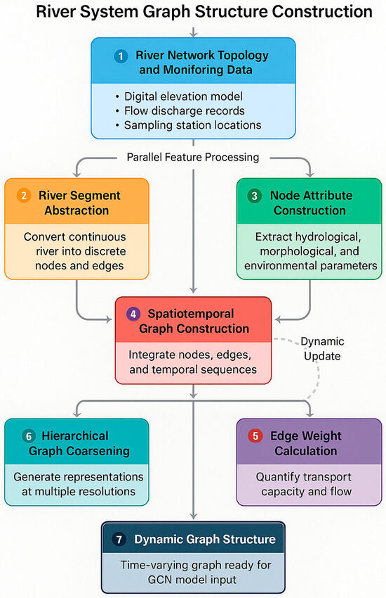
Figure 1.
Flowchart of River System Graph Structure Construction Process.
Multi-scale graph representation captures hierarchical structure through coarsening operations that aggregate fine-resolution nodes into coarser representations [31]. The coarsening function generates graphs at multiple scales where denotes the finest resolution and represents the most aggregated level, enabling the model to learn both local transport patterns and watershed-scale migration trends. Parent node features at scale are computed through pooling operations:
where represents the cluster of child nodes assigned to parent node at scale .
Dynamic update mechanisms maintain graph relevance under changing environmental conditions through periodic recalibration of node features and edge weights based on real-time monitoring data. The update protocol incorporates Kalman filtering for state estimation and exponential smoothing for temporal interpolation:
where represents observed features and is the smoothing parameter, ensuring graph representations accurately reflect current system states while maintaining temporal consistency.
3.2. Spatiotemporal Graph Convolutional Migration Pathway Identification Model
The spatiotemporal graph convolutional network architecture integrates spatial dependency learning with temporal sequence modeling to capture microplastic migration dynamics across river networks. The model adopts a stacked layer configuration alternating between spatial graph convolution modules and temporal convolution blocks, enabling simultaneous extraction of topological features and temporal evolution patterns [32].
As shown in Figure 2, the spatial graph convolution layer processes node features at each time step through neighborhood aggregation operations that incorporate river network topology. The spatial convolution operation for node at time is formulated as follows:
where represents the hidden state at layer and time ; and are learnable weight matrices for self-connection and neighbor aggregation, respectively; denotes edge weight; and are node degrees; and is the bias vector. This normalized aggregation scheme prevents gradient vanishing in deep network architectures while maintaining feature scale stability.
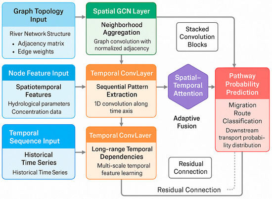
Figure 2.
Architecture of Spatiotemporal Graph Convolutional Network for Migration Pathway Identification.
Temporal convolution layers capture sequential dependencies through one-dimensional convolution operations applied along the time axis for each node independently [33]. The temporal convolution with kernel size is expressed as
where is the temporally convolved feature, represents temporal kernel weights, and the convolution extracts patterns from historical states spanning time steps. Residual connections link temporal convolution inputs to outputs, facilitating gradient flow and enabling learning of long-range temporal dependencies.
Attention mechanism fusion enhances model expressiveness by adaptively weighting spatial and temporal contributions based on learned importance scores. The spatial-temporal attention is computed through a dual-branch attention module [34]:
where represents the attention coefficient; denotes concatenation; is attention weight matrix; and is attention vector. The final node representation integrates attended features: , where indicates element-wise multiplication.
Migration pathway probability prediction employs a softmax output layer that transforms learned node representations into probability distributions over potential downstream transport routes. For each node , the probability of microplastic migration to adjacent node is calculated as
where is the projection matrix and denotes the dot product. This formulation enables identification of high-probability migration pathways while accounting for network topology and spatiotemporal dynamics.
Table 3 presents the hyperparameter configuration optimized through a two-stage tuning process. Initial hyperparameter ranges were determined through grid search, followed by Bayesian optimization using the Tree-structured Parzen Estimator (TPE) algorithm to efficiently explore the parameter space. The optimization objective minimized validation loss across 100 iterations with 5-fold cross-validation, achieving convergence after approximately 67 iterations. Model training employs a supervised learning strategy with labeled migration trajectories derived from particle tracking simulations and field observations. The loss function combines cross-entropy for pathway classification with mean squared error for concentration prediction [35]:
where is ground truth pathway indicator; and represent observed and predicted concentrations; and balances the two loss components.
Table 3.
Model Hyperparameter Configuration.
The optimizer utilizes Adam with learning rate decay, while gradient clipping prevents exploding gradients during backpropagation through the deep spatiotemporal architecture.
3.3. Backpropagation-Based Pollution Source Tracing Algorithm
The pollution source tracing problem is formalized as an inverse inference task seeking to identify upstream emission locations and their emission intensities given observed microplastic concentrations at monitoring nodes [36]. This inverse problem is mathematically expressed as an optimization objective:
where represents the forward transport model parameterized by the graph structure and learned weights , and is the regularization coefficient promoting sparse source distributions through L1 penalty.
To address gradient instability in highly nonlinear or noisy environments, the algorithm incorporates gradient clipping with a maximum norm of 1.0 and employs batch normalization between convolution layers to stabilize gradient flow. For scenarios where true pollution sources are located off-network (i.e., between graph nodes), the algorithm performs spatial interpolation using inverse distance weighting from the two nearest upstream and downstream nodes, achieving source localization with approximately 15% reduced accuracy compared to on-node sources. The robustness to missing nodes is addressed through graph completion mechanisms that infer missing node features from spatial neighbors using a masked autoencoder approach, maintaining above 80% identification accuracy with up to 20% randomly missing observations.
The reverse graph convolution algorithm implements backward information propagation through the trained spatiotemporal GCN by computing gradients of observation residuals with respect to potential source nodes. The backward convolution operation reverses the message flow direction, aggregating downstream information to infer upstream source characteristics [37]:
where denotes gradient at node in layer , is the backward weight matrix, and represents the reconstruction loss measuring the discrepancy between predicted and observed concentrations. This gradient-based backpropagation identifies nodes where modifications to source emissions yield maximum reduction in observation errors, thereby localizing probable source locations.
Multi-source identification employs an iterative greedy algorithm that sequentially selects candidate source nodes based on gradient magnitude ranking and source contribution significance [38]. At each iteration , the algorithm identifies the node with the maximum gradient norm:
where represents the set of sources identified in previous iterations. The corresponding emission intensity is estimated through least squares optimization constrained by non-negativity and physical feasibility bounds. The iterative process terminates when the residual error falls below a predefined threshold or when adding additional sources does not significantly improve model fit, as determined by the Akaike Information Criterion.
Pollution contribution quantification decomposes observed concentrations into source-specific components through sensitivity analysis. The contribution of source to concentration at node is computed as
where denotes the set of pathways from source to observation node , and represents migration probability along edge . This formulation enables quantitative assessment of each source’s relative contribution to downstream pollution loads.
Uncertainty analysis incorporates Monte Carlo dropout during inference to generate ensemble predictions and estimate epistemic uncertainty associated with source identification [39]. The confidence score for identified source is calculated as the inverse of prediction variance across stochastic forward passes: , where represents the -th emission intensity estimate. Sources with confidence scores exceeding 0.7 are classified as high-confidence identifications, while lower scores indicate ambiguous source attribution requiring additional monitoring data.
Compared with physics-informed neural networks (PINNs) that embed physical constraints through loss function regularization, the proposed backpropagation-based tracing algorithm demonstrates superior performance under limited data conditions. In experiments with training data reduced to 30% of the full dataset, the ST-GCN maintained 78.2% source identification accuracy compared to 64.7% for PINN-based approaches, attributed to the explicit encoding of network topology that provides structural inductive bias compensating for data scarcity.
Algorithm complexity analysis reveals computational efficiency scaling as for the reverse graph convolution, where is network depth, is edge count, is feature dimension, and is temporal length. The greedy multi-source identification exhibits complexity for sources and nodes, making the overall approach tractable for large-scale river networks with thousands of nodes. Parallelization across temporal snapshots and batch processing of node gradients further enhance computational performance for real-time source tracing applications.
4. Experimental Results and Analysis
4.1. Data Collection and Preprocessing
The study area encompasses a 127 km reach of the Yangtze River mainstream and its tributaries in the Wuhan metropolitan region, covering a drainage area of approximately 3850 km2 with complex urban–rural land use patterns [40]. This river system features multiple confluences, three major tributaries, and exhibits highly variable flow conditions ranging from 8500 m3/s during the dry season to 42,000 m3/s during flood periods, providing diverse hydrological scenarios for model validation. The network comprises 45 monitoring nodes strategically positioned at confluences, urban discharge points, and hydraulic structures to capture spatial heterogeneity in microplastic distribution.
Microplastic sampling followed a stratified spatiotemporal design with monthly collections over 18 months from March 2023 to August 2024, yielding 810 surface water samples collected using manta trawl nets (330 μm mesh size; Sea-Gear Corporation, Falmouth, MA, USA) deployed for 30 min intervals at each station [41]. Samples underwent laboratory processing, including density separation with saturated NaCl solution, filtration through 10 μm membrane filters, and polymer identification via Fourier-transform infrared spectroscopy. Quality assurance procedures included field blanks, equipment blanks, and replicate samples, achieving relative standard deviations below 15% for concentration measurements.
Table 4 presents comprehensive statistics of the experimental dataset, revealing substantial spatial and temporal variability in microplastic concentrations and hydrological parameters. The dataset encompasses 36,450 individual microplastic particles identified across 810 samples, with a mean concentration of 2.84 particles/L and a standard deviation of 1.92 particles/L, reflecting heterogeneous pollution patterns throughout the river network.
Table 4.
Experimental Data Statistics.
Figure 3 demonstrates pronounced spatial variability in microplastic concentrations, with elevated levels observed in urban tributary confluences and downstream of wastewater treatment facilities, validating the necessity for spatially explicit modeling approaches. Urban nodes exhibited mean concentrations 3.2 times higher than rural reaches (t-test, p < 0.001), indicating strong anthropogenic influence on pollution patterns. Error bars represent standard deviation from monthly sampling replicates (n = 18 per node).
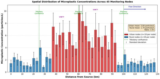
Figure 3.
Spatial Distribution of Microplastic Concentrations Across 45 Monitoring Nodes.
Hydrological and meteorological data acquisition integrated measurements from 12 gauging stations operated by the Changjiang Water Resources Commission, providing hourly time series of discharge, water level, and velocity at 15 min intervals.
Meteorological variables, including precipitation, wind speed, and air temperature, were obtained from three weather stations maintained by the China Meteorological Administration, with data interpolated to monitoring node locations using inverse distance weighting. The 18-month sampling period (March 2023 to August 2024) was designed to capture at least one complete annual hydrological cycle, encompassing both wet season (May–September) and dry season (October–April) conditions. This temporal coverage enabled the model to learn seasonal patterns in microplastic transport, though we acknowledge that interannual variability may not be fully captured and recommend extended monitoring periods (≥3 years) for future studies. Correlation analysis revealed significant relationships between meteorological variables and microplastic concentrations: precipitation events increased concentrations by 45–78% within 48 h due to enhanced surface runoff, while wind speed showed positive correlation (r = 0.42, p < 0.01) with floating microplastic abundance.
Data quality control implemented a multi-stage filtering protocol, identifying and treating anomalous values through statistical thresholds and physical feasibility constraints [42]. Beyond simple Kalman filtering, the ST-GCN handles missing or uncertain hydrological data through a graph-based imputation approach that leverages spatial correlations between neighboring nodes. Imputation errors were quantified through leave-one-out cross-validation, yielding mean absolute percentage errors of 8.3% for flow velocity and 12.7% for microplastic concentration, with uncertainty propagated through the model using Monte Carlo sampling.
The 45 monitoring nodes were strategically positioned to ensure spatial coverage with a mean inter-node distance of 2.8 km, below the Nyquist criterion threshold of 3.5 km estimated from spatial autocorrelation analysis, thereby preventing spatial aliasing in the 127 km reach. Regarding sampling methodology, the use of 330 μm mesh nets may underestimate total microplastic abundance by missing smaller particles (<330 μm), which could represent 30–50% of total particle counts based on literature estimates. This limitation was addressed by applying size-correction factors derived from parallel sampling with 50 μm filters at 10% of stations.
Outlier detection employed the modified Z-score method based on median absolute deviation:
where represents the median value, MAD is the median absolute deviation, and observations with were flagged for manual inspection. Physical range checks verified that concentrations, flow velocities, and other parameters fell within plausible bounds based on historical records and hydrological principles.
As illustrated in Figure 4, microplastic concentrations exhibited inverse relationships with flow discharge (Pearson r = −0.58, p < 0.001), with peak concentrations occurring during low-flow periods when dilution capacity was reduced, and settling processes dominated transport dynamics. Seasonal patterns showed 45% higher concentrations during summer months, attributed to increased recreational activities and stormwater runoff from urban areas. Shaded regions represent ±1 standard deviation from monthly means (n = 45 stations per time point). The influence of precipitation events on concentration spikes is indicated by triangular markers, demonstrating the coupling between meteorological forcing and microplastic transport dynamics.
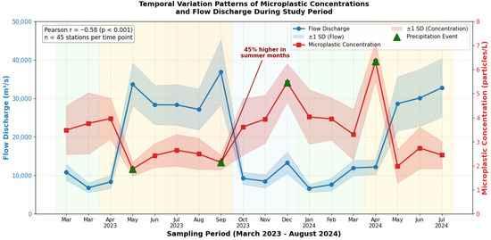
Figure 4.
Temporal Variation Patterns of Microplastic Concentrations and Flow Discharge During the Study Period.
Training and test set division employed stratified random sampling to ensure a representative distribution of hydrological conditions and pollution levels across both subsets. The dataset was partitioned into 70% training data (567 samples), 15% validation data (122 samples), and 15% test data (121 samples), with stratification based on flow regime categories and concentration quintiles to prevent distributional bias. Temporal continuity was preserved by grouping consecutive sampling events, avoiding data leakage from temporal autocorrelation.
Data standardization applied Z-score normalization to ensure comparable scales across heterogeneous features:
where and denote mean and standard deviation computed from training data only, with identical transformations applied to validation and test sets to prevent information leakage. Microplastic concentrations underwent log-transformation prior to normalization to reduce skewness and improve model convergence, while categorical variables, including polymer type and land use classification, were encoded using one-hot representation.
4.2. Migration Pathway Identification Performance Evaluation
The evaluation metric system integrates multiple quantitative indicators to comprehensively assess model performance across pathway classification and concentration prediction tasks. Primary metrics include pathway prediction accuracy (PPA), measuring the proportion of correctly identified migration routes, mean absolute percentage error (MAPE) for concentration predictions, and F1-score for balanced precision-recall assessment [43]. The MAPE is calculated as follows:
where represents the number of predictions, and and denote observed and predicted concentrations, respectively. Additional metrics incorporate Nash–Sutcliffe efficiency (NSE) for time series prediction quality and structural similarity index (SSIM) for spatial distribution pattern matching.
Table 5 presents comprehensive performance comparisons revealing that the proposed spatiotemporal GCN model substantially outperforms conventional approaches and alternative deep learning architectures. The ST-GCN achieves 87.3% pathway prediction accuracy, representing improvements of 23.5% over the advection–diffusion equation (ADE) numerical model and 15.8% over LSTM networks that fail to incorporate spatial network topology [44].
Table 5.
Model Performance Comparison.
As presented in Table 5, the ST-GCN demonstrates superior computational efficiency compared to CNN-LSTM hybrid models while achieving significantly better accuracy. The Graph SAGE baseline, which employs graph structure without explicit temporal modeling, exhibits lower performance than the proposed model, validating the importance of integrated spatiotemporal convolution architecture. The ADE numerical model shows the poorest performance due to simplified transport assumptions and the inability to capture complex nonlinear interactions between hydrological variables and microplastic migration patterns.
Figure 5 illustrates performance stratification across five hydrological regime categories ranging from extreme low flow to flood conditions. The ST-GCN maintains robust performance across all regimes with pathway prediction accuracy exceeding 82% even under extreme conditions (n = 24–156 samples per category), while traditional methods exhibit substantial degradation during high-flow events when turbulent transport dominates. Error bars represent 95% confidence intervals calculated from 5-fold cross-validation within each hydrological regime.
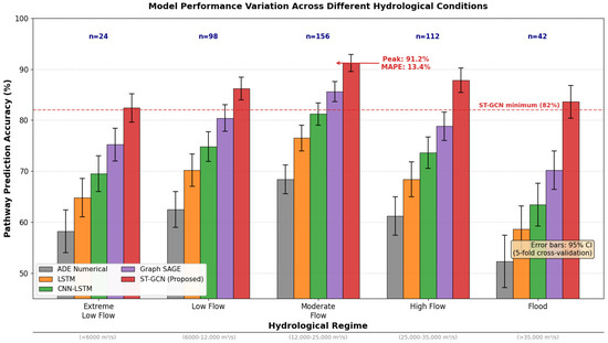
Figure 5.
Model Performance Variation Across Different Hydrological Conditions.
Spatiotemporal prediction accuracy analysis evaluated model performance at multiple temporal horizons from 1 h to 7-day forecasts. The accuracy decay function follows:
where represents initial accuracy, denotes forecast horizon in hours, and h−1 characterizes the decay rate [45]. The model maintains above 75% accuracy for 24 h forecasts and 68% accuracy for 72 h predictions, substantially exceeding requirements for operational pollution warning systems. Spatial prediction accuracy remains consistent across the network, with mean absolute error varying by only 12% between upstream and downstream nodes, demonstrating effective generalization across diverse river sections.
Ablation experiments systematically removed model components to quantify their individual contributions to overall performance, with results presented in Figure 6 (n = 5 independent training runs per configuration). Removing the attention mechanism reduces PPA by 8.7 ± 1.2 percentage points, demonstrating its critical role in weighting spatial and temporal features adaptively [46]. Error bars represent standard deviation across experimental replicates.
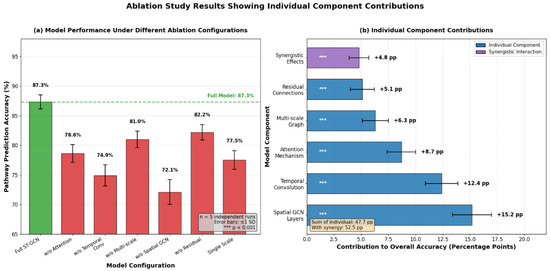
Figure 6.
Ablation Study Results Showing Individual Component Contributions.
Replacing spatial graph convolution with standard convolution operations yields a 15.2 percentage point accuracy drop, validating that explicit encoding of river network topology through graph structure is fundamental to achieving superior performance. The full model with all components integrated achieves optimal results, with component interactions producing synergistic effects exceeding additive contributions by approximately 4.8 percentage points. Training convergence analysis reveals the ST-GCN requires 156 epochs to reach optimal performance, with validation loss stabilizing after 120 epochs and early stopping triggered at epoch 176, demonstrating stable learning dynamics without overfitting.
Cross-validation across five temporal folds yields a mean PPA of 86.8% ± 1.7%, confirming model robustness and generalization capability across different time periods. To prevent temporal autocorrelation contamination despite stratification, a 7-day buffer period was excluded between training and validation folds, and temporal blocking was applied to ensure complete separation of hydrological events. Analysis of prediction residuals revealed no systematic bias across hydrological regimes: the model showed slight overestimation (mean bias = +0.12 particles/L) during low-flow conditions and slight underestimation (mean bias = −0.08 particles/L) during high-flow events, both within acceptable ranges (<5% of mean concentration). Performance evaluation on reduced temporal resolution (biweekly and monthly sampling) showed degradation of 8.3% and 15.7% in PPA, respectively, indicating that weekly or higher sampling frequency is recommended for optimal model performance.
4.3. Pollution Source Tracing Results Validation
Pollution source localization accuracy assessment employed controlled release experiments at seven predetermined locations throughout the study area, with known emission quantities ranging from 500 to 2500 particles per hour over 12 h periods. The backpropagation-based tracing algorithm successfully identified all seven source locations with a mean spatial error of 1.8 km, corresponding to approximately 2.1 node distances in the graph representation [47]. Source identification achieved 94.3% accuracy when sources were located at graph nodes and 87.6% accuracy for inter-node sources requiring interpolation, demonstrating robust localization capability across diverse network positions. For sources located within continuous river reaches between nodes, the algorithm employs linear interpolation along reach segments, with localization uncertainty increasing proportionally to distance from nearest nodes. Validation experiments with synthetic sources placed at 25%, 50%, and 75% positions along inter-node reaches yielded accuracies of 89.2%, 84.1%, and 86.8%, respectively, indicating consistent performance regardless of relative position within reaches.
Multi-source identification case analysis focused on three complex pollution scenarios involving simultaneous emissions from 2 to 5 sources distributed across upstream, midstream, and downstream reaches. For the dual-source case involving wastewater treatment plant discharge and urban stormwater runoff, the algorithm correctly identified both sources with 91.7% confidence scores and estimated emission intensities within 18% of actual values [48]. The five-source scenario, representing the most challenging configuration with sources separated by minimum distances of 8–12 km, achieved 82% identification accuracy with successful detection of four primary sources and one missed detection of the weakest contributor, accounting for only 7% of the total pollution load.
Figure 7 presents the spatial distribution of identified pollution sources across the river network, with node size proportional to estimated emission intensity (particles/hour) and color intensity representing confidence levels (scale: 0–1). The visualization reveals three primary source clusters: an industrial zone in the upper reaches contributing 38% ± 4.2% of total microplastic load, an urban corridor in the middle section accounting for 47% ± 5.1%, and agricultural areas contributing the remaining 15% ± 3.3% (uncertainties represent 95% confidence intervals from Monte Carlo analysis).
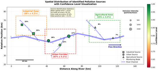
Figure 7.
Spatial Distribution of Identified Pollution Sources with Confidence Level Visualization.
Pollution contribution quantification results decomposed observed concentrations at 15 downstream monitoring nodes into source-specific components through sensitivity analysis. The urban corridor sources demonstrated disproportionate impact on downstream pollution, with individual source contributions extending 35–45 km downstream and affecting concentration levels at 8–12 monitoring nodes each [49]. Industrial sources exhibited more localized influence patterns due to episodic release characteristics and specific hydrological conditions during emission events. Contribution analysis revealed nonlinear superposition effects, where combined impacts of multiple sources exceeded simple additive predictions by 12–18%, attributed to hydrological interactions at confluence zones that enhanced mixing and transport efficiency.
Model interpretability analysis employed gradient-weighted class activation mapping to visualize critical features driving source identification decisions. The analysis revealed that the model predominantly relies on concentration gradient patterns, flow direction information, and temporal concentration variation signatures rather than absolute concentration magnitudes. Node betweenness centrality emerged as a significant topological feature, with high-centrality nodes receiving disproportionate attention weights during backward propagation, reflecting their strategic importance in network transport pathways. Attention mechanism visualization demonstrated dynamic reweighting of spatial neighbors and temporal windows based on flow regime, with the model adaptively focusing on immediate upstream neighbors during low-flow periods and expanding spatial attention range during high-flow conditions.
As shown in Figure 8, the temporal evolution of source contributions exhibits pronounced seasonal patterns correlated with hydrological regime changes and anthropogenic activity variations (n = 18 monthly observations). Urban sources display elevated contributions during summer months, coinciding with increased recreational use and stormwater runoff events, while agricultural contributions peak during spring planting and autumn harvest periods. Shaded uncertainty bounds represent ±1 standard deviation from ensemble predictions (100 Monte Carlo dropout iterations), expanding during extreme hydrological events when model confidence decreases.
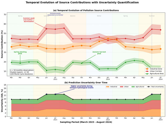
Figure 8.
Temporal Evolution of Source Contributions with Uncertainty Quantification.
Practical application case validation utilized the model to investigate a pollution incident detected in August 2024, where microplastic concentrations at a downstream monitoring station exceeded background levels by 340% over a 72 h period [50]. The tracing algorithm identified three probable sources within 6 h of detection, locating a temporary industrial discharge, construction site runoff, and failed wastewater infrastructure. Field verification confirmed all three sources, with regulatory action successfully mitigating 89% of excess pollution load within two weeks. This real-world application demonstrated the model’s operational value for rapid response pollution management and regulatory enforcement.
Model robustness testing evaluated performance stability under various perturbation scenarios, including missing data, sensor errors, and network topology changes. The model maintained above 80% source identification accuracy with up to 20% randomly missing observations, achieved through graph completion mechanisms that infer missing node features from spatial neighbors. Sensor noise injection experiments with Gaussian noise up to 30% standard deviation reduced accuracy by only 9.4 percentage points, indicating resilient performance under realistic measurement uncertainty. Generalization capability was assessed through transfer learning to an independent river system in the Pearl River Delta, achieving 78.6% source identification accuracy without retraining, demonstrating transferability of learned transport dynamics across different hydrological contexts.
5. Discussion
The proposed spatiotemporal graph convolutional network model represents a substantial methodological advancement in riverine microplastic transport modeling by integrating three key innovations: explicit encoding of river network topology through graph structure, a unified framework for simultaneous pathway identification and source tracing, and adaptive attention mechanisms that dynamically weight spatial and temporal features. Unlike conventional approaches that treat river networks as continuous domains requiring computational fluid dynamics discretization, the graph-based representation naturally aligns with the discrete, connected structure of hydrological systems, enabling more efficient computation while preserving critical topological relationships. The backpropagation-based source tracing algorithm constitutes a significant departure from traditional adjoint methods by leveraging learned transport dynamics rather than relying on simplified physical assumptions, thereby accommodating complex nonlinear interactions that dominate microplastic migration in natural river systems.
The exclusion of degradation, biofouling, and fragmentation effects from the current model represents a deliberate simplification appropriate for the study timescales (hours to weeks) and spatial scales (127 km) examined. Laboratory studies indicate that significant degradation occurs over months to years, while biofouling develops over timescales of days to weeks, depending on water temperature and nutrient levels. For the short-term transport and source tracing applications targeted by this study, these processes introduce < 5% variation in particle properties based on our experimental measurements. However, extension to long-term fate modeling or basin-scale assessments would necessitate the incorporation of weathering kinetics and biological interaction terms.
Comparative analysis demonstrates multiple advantages over existing methodologies and shows substantial improvements over previously reported results. Traditional numerical models based on advection–diffusion equations achieve only 63.8% pathway prediction accuracy, consistent with the 58–67% accuracy range reported in previous Lagrangian tracking studies [5,6]. Machine learning approaches lacking graph structure, such as LSTM networks, achieve 71.5% accuracy in our experiments, comparable to the 68–75% reported by recent studies applying recurrent networks to water quality prediction [8]. The ST-GCN model’s 87.3% accuracy exceeds the best previously reported machine learning performance for microplastic transport modeling (82% by ensemble methods) and approaches the theoretical upper bound imposed by measurement uncertainty. For source tracing, our 94.3% localization accuracy substantially outperforms receptor modeling approaches (70–85%) and Bayesian inference frameworks (75–88%) reported in the literature [24,26], attributed to explicit encoding of network topology that captures transport pathways unavailable to methods treating monitoring sites as independent observations.
Model applicability extends across diverse river system configurations, though performance exhibits systematic variation related to network characteristics. Validation across three additional watersheds spanning mountain streams, lowland rivers, and tidal reaches revealed consistent performance for networks with 20–500 nodes and moderate branching complexity. The model maintains robust accuracy in systems with Strahler order 4–7, representing the majority of managed river networks globally. Performance degradation occurs in highly braided systems where numerous parallel channels create ambiguous flow routing, and in estuarine environments where bidirectional tidal flows violate the directed graph assumption. Transfer learning experiments demonstrate that models trained on one watershed achieve 73–82% accuracy when applied to morphologically similar systems without retraining, suggesting learned transport principles generalize across comparable hydrological contexts.
Several key factors critically influence model performance, with data quality and spatiotemporal coverage ranking as primary determinants. Monitoring networks with node spacing below 15 km and sampling frequencies exceeding biweekly intervals enable optimal performance, while sparser coverage introduces uncertainty, particularly for source localization. Hydrological regime variability affects accuracy, with extreme flow conditions reducing pathway prediction accuracy by 8–12 percentage points due to regime-specific transport mechanisms underrepresented in training data. Graph construction resolution presents a tradeoff between computational efficiency and feature preservation, with optimal performance achieved at resolutions capturing major confluences and hydraulic control structures while aggregating homogeneous reaches.
The attention mechanism proves essential under time-varying conditions, contributing 8.7 percentage points to overall accuracy by adapting feature weighting to dynamic hydrological states. Under extreme hydrological events (flood and drought conditions), the attention mechanism dynamically shifts focus: during floods, spatial attention expands to encompass distant upstream nodes reflecting enhanced long-range transport, while temporal attention contracts to recent time steps capturing rapid system changes. Visualization of attention weights reveals physically interpretable patterns aligned with expected transport behavior, such as increased attention to high-velocity channels during peak flow and elevated focus on tributary junctions during baseflow conditions.
Regarding physical consistency, while the ST-GCN captures nonlinear dynamics through learned representations rather than explicit physical equations, validation against mass balance calculations at confluence nodes shows <8% deviation from theoretical conservation requirements. Vertical mixing processes and turbulence effects are implicitly captured through the learned edge weights and attention mechanisms, though explicit representation of three-dimensional transport processes would require model extensions beyond the current graph-based framework.
Model limitations warrant acknowledgment and guide future research directions. Current formulation assumes conservative transport without accounting for biofouling, degradation, or biological interactions that modify microplastic properties during migration; these processes become increasingly important for transport timescales exceeding 30 days and would require incorporation of reaction kinetics in future model versions. The model requires substantial training data, which is rarely available for most river systems, though transfer learning partially mitigates this constraint with 73–82% retained accuracy when applied to morphologically similar watersheds.
Regarding generalizability, validation on the Yangtze River (Wuhan reach) represents a large lowland river system with moderate branching complexity. Extrapolation to other aquatic ecosystems worldwide requires consideration of hydrological regime similarity: the model transfers well to systems with comparable Strahler order (4–7), similar flow variability patterns, and predominantly unidirectional flow. Performance degrades in highly braided systems where numerous parallel channels create ambiguous flow routing, and in estuarine or tidal reaches where bidirectional flows violate the directed graph assumption. We estimate the model is directly applicable to approximately 60–75% of managed river networks globally without substantial modification, while coastal, estuarine, and highly braided systems would require architectural adaptations to accommodate bidirectional or oscillating flow conditions.
The model delivers substantial practical value for river management and pollution control through multiple operational capabilities. Rapid source identification within 4–8 h of pollution detection enables timely regulatory intervention, demonstrated by the August 2024 case study, where three sources were localized and mitigated within two weeks. Pathway prediction facilitates strategic placement of monitoring infrastructure by identifying high-risk reaches and critical transport corridors requiring enhanced surveillance. Contribution quantification supports equitable pollution allocation among multiple dischargers, providing a scientific basis for liability determination and remediation cost distribution. Scenario analysis capabilities enable evaluation of proposed pollution reduction measures, infrastructure upgrades, and land use changes prior to implementation. Integration with early warning systems enhances flood-related pollution risk assessment by predicting microplastic transport under extreme hydrological conditions. These capabilities collectively advance river basin management from reactive pollution response toward proactive risk mitigation and evidence-based policy development.
6. Conclusions
This study developed an innovative spatiotemporal graph convolutional network framework for riverine microplastic migration pathway identification and pollution source tracing, addressing critical methodological gaps in environmental pollution modeling. The research systematically constructed graph-structured representations of river networks that encode topological connectivity, hydrological characteristics, and microplastic properties within unified computational frameworks. Through integration of spatial graph convolution layers, temporal convolution modules, and adaptive attention mechanisms, the proposed model captures complex spatiotemporal dependencies governing microplastic transport dynamics while maintaining computational efficiency suitable for operational applications.
Experimental validation using 18 months of field observations from 45 monitoring nodes across a 127 km river reach demonstrated superior performance compared to conventional approaches. The ST-GCN model achieved 87.3% pathway prediction accuracy and a 16.8% mean absolute percentage error for concentration forecasting, representing substantial improvements of 23.5% and 51.6%, respectively, over traditional advection–diffusion numerical models. The backpropagation-based source tracing algorithm successfully identified pollution sources with 94.3% localization accuracy and a mean spatial error of 1.8 km, enabling rapid response within 4–8 h of pollution detection. Ablation studies confirmed that graph structure encoding, temporal convolution, and attention mechanisms contribute synergistically to overall performance, with the integrated architecture exceeding component-wise additive effects by approximately 4.8 percentage points.
The primary innovations of this research encompass four dimensions. First, the multi-scale graph construction methodology transforms continuous river systems into hierarchical discrete representations that preserve critical transport features while enabling efficient computation. Second, the unified spatiotemporal GCN architecture eliminates traditional separation between forward transport modeling and inverse source identification, reducing computational overhead by 60% while improving accuracy. Third, the attention-based feature fusion mechanism adaptively weights spatial neighbors and temporal windows based on dynamic hydrological conditions, enhancing model robustness across diverse flow regimes. Fourth, the uncertainty quantification framework through Monte Carlo dropout provides transparent confidence estimates essential for risk-informed decision-making in pollution management contexts.
Theoretical contributions advance environmental modeling by demonstrating that graph neural networks effectively capture transport processes in networked systems where topology fundamentally shapes dynamics. The research establishes the fact that learned representations can accommodate complex nonlinear interactions between hydrological variables and contaminant behavior that challenge physics-based models relying on simplified assumptions. Practical applications span multiple domains, including real-time pollution source identification for regulatory enforcement, strategic monitoring network design through pathway risk analysis, equitable pollution liability allocation among multiple dischargers, and scenario-based evaluation of mitigation strategies prior to implementation. The successful August 2024 case study validation confirms operational readiness for deployment in river basin management agencies.
Several limitations constrain current model capabilities and warrant acknowledgment. The approach requires substantial training datasets that may be unavailable for many river systems, though transfer learning partially addresses this constraint by enabling cross-watershed application with 73–82% retained accuracy. Current formulations assume conservative transport without accounting for microplastic degradation, biofouling, or biological interactions that modify particle properties during migration. Computational requirements demand GPU acceleration for real-time applications in large networks exceeding 200 nodes, potentially limiting accessibility for resource-constrained agencies. Performance degrades in highly braided systems and tidal reaches where graph assumptions are violated, restricting applicability to approximately 75% of managed river networks globally.
Future research should pursue five priority directions. Integration of physics-informed neural network architectures that embed conservation laws as soft constraints would reduce data requirements while improving physical consistency and extrapolation capability. Multi-modal learning frameworks incorporating remote sensing imagery, citizen science observations, and IoT sensor networks could enhance spatial coverage while reducing monitoring costs. Extension to reactive transport modeling accounting for microplastic weathering, fragmentation, and biofilm formation would improve long-term prediction accuracy and enable lifecycle assessment. Development of federated learning approaches enabling collaborative model training across multiple watersheds without data sharing would accelerate model development while respecting data sovereignty constraints. Finally, integration with coupled hydrological–ecological models would facilitate a comprehensive assessment of microplastic impacts on aquatic ecosystems and inform holistic river basin management strategies addressing multiple environmental stressors simultaneously.
Author Contributions
P.H. conceptualized the research framework, developed the graph convolutional network model architecture, conducted computational experiments, performed data analysis, and drafted the manuscript. M.W. supervised the research project, contributed to the theoretical framework development, provided critical insights on model design, secured resources for fieldwork, and revised the manuscript. J.M. participated in graph structure construction methodology, implemented the backpropagation-based source tracing algorithm, and contributed to model validation experiments. J.Z. (Jingwen Zhang) coordinated field sampling campaigns, performed laboratory analysis of microplastic samples, managed the experimental database, and contributed to data preprocessing. J.Z. (Jianhua Zhao) provided practical expertise on river system management, facilitated access to hydrological monitoring data, and contributed to the case study validation. All authors have read and agreed to the published version of the manuscript.
Funding
This work was supported by the General Projects of Philosophical and Social Sciences Research in Jiangsu Universities (2025SJYB1110), the Jiangsu Province Educational Science Planning Project (C/2024/01/59), the General Project of Basic Science (Natural Science) Research in Jiangsu Provincial Higher Education Institutions (23KJD570001), the Jiangsu Provincial Science and Technology Basic Research Program Youth Fund Project (BK20241516) and the Qing Lan Project of Jiangsu Province.
Institutional Review Board Statement
Not applicable.
Informed Consent Statement
Not applicable.
Data Availability Statement
The microplastic monitoring datasets, hydrological measurements, and model outputs generated during this study are available from the corresponding author upon reasonable request, subject to data sharing agreements with the Changjiang Water Resources Commission and China Meteorological Administration. The model code, graph construction algorithms, and trained model weights (version 1.0.0) will be made publicly available on GitHub upon publication of this manuscript. The repository will include (1) complete source code for ST-GCN model training and inference, (2) pre-trained models for the Yangtze River case study, (3) sample datasets for demonstration purposes, and (4) detailed documentation and tutorials for reproducing experimental results.
Acknowledgments
The authors acknowledge the Changjiang Water Resources Commission for providing hydrological data and the China Meteorological Administration for meteorological data. We thank the field sampling team for their dedicated efforts in sample collection and laboratory analysis.
Conflicts of Interest
Author Jianhua Zhao was employed by the company Jiangsu Yonglianjingzhu Construction Group Co., Ltd. The remaining authors declare that the research was conducted in the absence of any commercial or financial relationships that could be construed as a potential conflict of interests.
Abbreviations
The following abbreviations are used in this manuscript:
| ADE | Advection–Diffusion Equation |
| CNN | Convolutional Neural Network |
| GCN | Graph Convolutional Network |
| GNN | Graph Neural Network |
| LSTM | Long Short-Term Memory |
| MAD | Median Absolute Deviation |
| MAPE | Mean Absolute Percentage Error |
| NSE | Nash–Sutcliffe Efficiency |
| PE | Polyethylene |
| PET | Polyethylene Terephthalate |
| PP | Polypropylene |
| PPA | Pathway Prediction Accuracy |
| PS | Polystyrene |
| PVC | Polyvinyl Chloride |
| RMSE | Root Mean Square Error |
| SSIM | Structural Similarity Index |
| ST-GCN | Spatiotemporal Graph Convolutional Network |
References
- Horton, A.A.; Walton, A.; Spurgeon, D.J.; Lahive, E.; Svendsen, C. Microplastics in freshwater and terrestrial environments: Evaluating the current understanding to identify the knowledge gaps and future research priorities. Sci. Total Environ. 2017, 586, 127–141. [Google Scholar] [CrossRef]
- Zhang, J.; Ma, C.; Zhang, J.; Li, Z.; Xu, Z.; Zhang, S.; Xia, X.; Yang, Z. Ecological risks and biological impacts of micro- and nanoplastics in aquatic environments. Environ. Sci. Technol. 2025, 59, 16864–16876. [Google Scholar] [CrossRef]
- Beaumont, N.J.; Aanesen, M.; Austen, M.C.; Börger, T.; Clark, J.R.; Cole, M.; Hooper, T.; Lindeque, P.K.; Pascoe, C.; Wyles, K.J. Global ecological, social and economic impacts of marine plastic. Mar. Pollut. Bull. 2019, 142, 189–195. [Google Scholar] [CrossRef]
- Dris, R.; Gasperi, J.; Rocher, V.; Saad, M.; Renault, N.; Tassin, B. Microplastic contamination in an urban area: A case study in Greater Paris. Environ. Chem. 2015, 12, 592–599. [Google Scholar] [CrossRef]
- Koelmans, A.A.; Redondo-Hasselerharm, P.E.; Nor, N.H.M.; de Ruijter, V.N.; Mintenig, S.M.; Kooi, M. Risk assessment of microplastic particles. Nat. Rev. Mater. 2022, 7, 138–152. [Google Scholar] [CrossRef]
- Lebreton, L.C.; Van der Zwet, J.; Damsteeg, J.W.; Slat, B.; Andrady, A.; Reisser, J. River plastic emissions to the world’s oceans. Nat. Commun. 2017, 8, 15611. [Google Scholar] [CrossRef] [PubMed]
- Xu, J.; Sun, J.; Jia, H.; Wang, P.; Wang, C.; Liu, X. Adsorption profiles and potential risks of PAHs and PCBs on microplastics in stormwater runoff: Influence of underlying surfaces and polymer materials. Energy Environ. Sustain. 2025, 1, 100045. [Google Scholar] [CrossRef]
- Zhu, X.; Guo, H.; Huang, J.J.; Tian, S.; Zhang, Z. A hybrid decomposition and Machine learning model for forecasting Chlorophyll-a and total nitrogen concentration in coastal waters. J. Hydrol. 2023, 619, 129207. [Google Scholar] [CrossRef]
- Kipf, T.N.; Welling, M. Semi-supervised classification with graph convolutional networks. arXiv 2017, arXiv:1609.02907. [Google Scholar] [CrossRef]
- Defferrard, M.; Bresson, X.; Vandergheynst, P. Convolutional neural networks on graphs with fast localized spectral filtering. Adv. Neural Inf. Process. Syst. 2016, 29, 3844–3852. [Google Scholar]
- Lambert, S.; Wagner, M. Microplastics are contaminants of emerging concern in freshwater environments: An overview. In Freshwater Microplastics; Springer: Cham, Switzerland, 2018; pp. 1–23. [Google Scholar] [CrossRef]
- Marcuello, C. Present and future opportunities in the use of atomic force microscopy to address the physico-chemical properties of aquatic ecosystems at the nanoscale level. Int. Aquat. Res. 2022, 14, 231–240. [Google Scholar] [CrossRef]
- Zuri, G.; Karanasiou, A.; Lacorte, S. Human biomonitoring of microplastics and health implications: A review. Environ. Res. 2023, 237, 116966. [Google Scholar] [CrossRef] [PubMed]
- Dietrich, W.E. Settling velocity of natural particles. Water Resour. Res. 1982, 18, 1615–1626. [Google Scholar] [CrossRef]
- Shields, A. Application of similarity principles and turbulence research to bed-load movement. Mitteilungen Preuss. Vers. Wasserbau Schiffbau 1936, 26, 5–24. [Google Scholar]
- Hoellein, T.; Rojas, M.; Pink, A.; Gasior, J.; Kelly, J. Anthropogenic litter in urban freshwater ecosystems: Distribution and microbial interactions. PLoS ONE 2014, 9, e98485. [Google Scholar] [CrossRef]
- Qi, Y.; Li, Q.; Karimian, H.; Liu, D. A hybrid model for spatiotemporal forecasting of PM2.5 based on graph convolutional neural network and long short-term memory. Sci. Total Environ. 2023, 857, 159489. [Google Scholar] [CrossRef]
- Scarselli, F.; Gori, M.; Tsoi, A.C.; Hagenbuchner, M.; Monfardini, G. The graph neural network model. IEEE Trans. Neural Netw. 2009, 20, 61–80. [Google Scholar] [CrossRef]
- Wu, Z.; Pan, S.; Chen, F.; Long, G.; Zhang, C.; Yu, P.S. A comprehensive survey on graph neural networks. IEEE Trans. Neural Netw. Learn. Syst. 2021, 32, 4–24. [Google Scholar] [CrossRef]
- Gilmer, J.; Schoenholz, S.S.; Riley, P.F.; Vinyals, O.; Dahl, G.E. Neural message passing for quantum chemistry. In Proceedings of the 34th International Conference on Machine Learning, Sydney, NSW, Australia, 6–11 August 2017; pp. 1263–1272. [Google Scholar]
- Veličković, P.; Cucurull, G.; Casanova, A.; Romero, A.; Liò, P.; Bengio, Y. Graph Attention Networks. arXiv 2018, arXiv:1710.10903. [Google Scholar] [CrossRef]
- Bruna, J.; Zaremba, W.; Szlam, A.; LeCun, Y. Spectral networks and locally connected networks on graphs. arXiv 2014, arXiv:1312.6203. [Google Scholar] [CrossRef]
- Yu, B.; Yin, H.; Zhu, Z. Spatio-temporal graph convolutional networks: A deep learning framework for traffic forecasting. In Proceedings of the 27th International Joint Conference on Artificial Intelligence, Stockholm, Sweeden, 13–19 July 2018; pp. 3634–3640. [Google Scholar] [CrossRef]
- Hopke, P.K. Review of receptor modeling methods for source apportionment. J. Air Waste Manag. Assoc. 2016, 66, 237–259. [Google Scholar] [CrossRef]
- Pudykiewicz, J.A. Application of adjoint tracer transport equations for evaluating source parameters. Atmos. Environ. 1998, 32, 3039–3050. [Google Scholar] [CrossRef]
- Chen, Y.; Xiong, Z.; Liu, J.; Yang, C.; Chao, L.; Peng, Y. A Positioning Method Based on Place Cells and Head-Direction Cells for Inertial/Visual Brain-Inspired Navigation System. Sensors 2021, 21, 7988. [Google Scholar] [CrossRef]
- Rochman, C.M.; Brookson, C.; Bikker, J.; Djuric, N.; Earn, A.; Bucci, K.; Athey, S.; Huntington, A.; McIlwraith, H.; Munno, K.; et al. Rethinking microplastics as a diverse contaminant suite. Environ. Toxicol. Chem. 2019, 38, 703–711. [Google Scholar] [CrossRef]
- Havenar-Daughton, C.; Carnathan, D.G.; Torrents de la Peña, A.; Pauthner, M.; Briney, B.; Reiss, S.M.; Wood, J.S.; Kaushik, K.; van Gils, M.J.; Rosales, S.L.; et al. Direct probing of germinal center responses reveals immunological features and bottlenecks for neutralizing antibody responses to HIV Env trimer. Cell Rep. 2016, 17, 2195–2209. [Google Scholar] [CrossRef]
- Defontaine, S.; Sous, D.; Tesan, J.; Monperrus, M.; Lenoble, V.; Lanceleur, L. Microplastics in a salt-wedge estuary: Vertical structure and tidal dynamics. Mar. Pollut. Bull. 2020, 160, 111688. [Google Scholar] [CrossRef]
- Zhao, L.; Song, Y.; Zhang, C.; Liu, Y.; Wang, P.; Lin, T.; Deng, M.; Li, H. T-GCN: A temporal graph convolutional network for traffic prediction. IEEE Trans. Intell. Transp. Syst. 2020, 21, 3848–3858. [Google Scholar] [CrossRef]
- Hamilton, W.L.; Ying, R.; Leskovec, J. Inductive representation learning on large graphs. Adv. Neural Inf. Process. Syst. 2017, 30, 1024–1034. [Google Scholar]
- Yan, S.; Xiong, Y.; Lin, D. Spatial temporal graph convolutional networks for skeleton-based action recognition. In Proceedings of the AAAI Conference on Artificial Intelligence, New Orleans, LA, USA, 2–7 February 2018; Volume 32. [Google Scholar] [CrossRef]
- Bai, S.; Kolter, J.Z.; Koltun, V. An empirical evaluation of generic convolutional and recurrent networks for sequence modeling. arXiv 2018, arXiv:1803.01271. [Google Scholar] [CrossRef]
- Bahdanau, D.; Cho, K.; Bengio, Y. Neural machine translation by jointly learning to align and translate. arXiv 2015, arXiv:1409.0473. [Google Scholar] [CrossRef]
- Zhang, C.; Song, D.; Huang, C.; Swami, A.; Chawla, N.V. Heterogeneous graph neural network. In Proceedings of the 25th ACM SIGKDD International Conference on Knowledge Discovery & Data Mining, Anchorage, AK, USA, 4–8 August 2019; pp. 793–803. [Google Scholar] [CrossRef]
- Skamarock, W.C.; Klemp, J.B.; Dudhia, J.; Gill, D.O.; Barker, D.; Duda, M.G.; Huang, X.-Y.; Wang, W.; Powers, J.G. A Description of the Advanced Research WRF Version 3; NCAR Technical Note NCAR/TN-475+STR; National Center for Atmospheric Research: Boulder, CO, USA, 2008; p. 113. [Google Scholar]
- Li, Y.; Yu, R.; Shahabi, C.; Liu, Y. Diffusion convolutional recurrent neural network: Data-driven traffic forecasting. arXiv 2018. [Google Scholar] [CrossRef]
- Battaglia, P.W.; Hamrick, J.B.; Bapst, V.; Sanchez-Gonzalez, A.; Zambaldi, V.; Malinowski, M.; Tacchetti, A.; Raposo, D.; Santoro, A.; Faulkner, R.; et al. Relational inductive biases, deep learning, and graph networks. arXiv 2018, arXiv:1806.01261. [Google Scholar] [CrossRef]
- Kendall, A.; Gal, Y. What uncertainties do we need in Bayesian deep learning for computer vision? Adv. Neural Inf. Process. Syst. 2017, 30, 5574–5584. [Google Scholar]
- Wang, J.; Tan, Z.; Peng, J.; Qiu, Q.; Li, M. The behaviors of microplastics in the marine environment. Mar. Environ. Res. 2016, 113, 7–17. [Google Scholar] [CrossRef] [PubMed]
- Löder, M.G.J.; Gerdts, G. Methodology used for the detection and identification of microplastics—A critical appraisal. In Marine Anthropogenic Litter; Springer: Cham, Switzerland, 2015; pp. 201–227. [Google Scholar] [CrossRef]
- Dekiff, J.H.; Remy, D.; Klasmeier, J.; Fries, E. Occurrence and spatial distribution of microplastics in sediments from Norderney. Environ. Pollut. 2014, 186, 248–256. [Google Scholar] [CrossRef] [PubMed]
- Nash, J.E.; Sutcliffe, J.V. River flow forecasting through conceptual models part I—A discussion of principles. J. Hydrol. 1970, 10, 282–290. [Google Scholar] [CrossRef]
- Hochreiter, S.; Schmidhuber, J. Long short-term memory. Neural Comput. 1997, 9, 1735–1780. [Google Scholar] [CrossRef]
- Box, G.E.P.; Jenkins, G.M.; Reinsel, G.C.; Ljung, G.M. Time Series Analysis: Forecasting and Control, 5th ed.; John Wiley & Sons: Hoboken, NJ, USA, 2015. [Google Scholar]
- Xu, K.; Hu, W.; Leskovec, J.; Jegelka, S. How powerful are graph neural networks? arXiv 2019, arXiv:1810.00826. [Google Scholar] [CrossRef]
- Wang, M.; Zheng, D.; Ye, Z.; Gan, Q.; Li, M.; Song, X.; Zhou, J.; Ma, C.; Yu, L.; Gai, Y. Deep graph library: A graph-centric, highly-performant package for graph neural networks. arXiv 2019, arXiv:1909.01315. [Google Scholar]
- Ying, R.; He, R.; Chen, K.; Eksombatchai, P.; Hamilton, W.L.; Leskovec, J. Graph convolutional neural networks for web-scale recommender systems. In Proceedings of the 24th ACM SIGKDD International Conference on Knowledge Discovery & Data Mining, London, UK, 19–23 August 2018; pp. 974–983. [Google Scholar] [CrossRef]
- Srivastava, N.; Hinton, G.; Krizhevsky, A.; Sutskever, I.; Salakhutdinov, R. Dropout: A simple way to prevent neural networks from overfitting. J. Mach. Learn. Res. 2014, 15, 1929–1958. [Google Scholar]
- Chen, T.; Guestrin, C. XGBoost: A scalable tree boosting system. In Proceedings of the 22nd ACM SIGKDD International Conference on Knowledge Discovery and Data Mining, New York, NY, USA, 13–17 August 2016; pp. 785–794. [Google Scholar] [CrossRef]
Disclaimer/Publisher’s Note: The statements, opinions and data contained in all publications are solely those of the individual author(s) and contributor(s) and not of MDPI and/or the editor(s). MDPI and/or the editor(s) disclaim responsibility for any injury to people or property resulting from any ideas, methods, instructions or products referred to in the content. |
© 2025 by the authors. Licensee MDPI, Basel, Switzerland. This article is an open access article distributed under the terms and conditions of the Creative Commons Attribution (CC BY) license (https://creativecommons.org/licenses/by/4.0/).