Seasonal Variability in the Impacts of Climatic and Landscape Dynamics on Soil Conservation Services: A Case Study from Upper and Middle Yellow River Basin, China

Abstract

A comprehensive understanding of the spatial and temporal dynamics of soil conservation (SC) and its driving mechanisms is vital for mitigating land degradation and developing erosion-control strategies. However, the influence of driving factors is time-scale dependent and spatially heterogeneous, which remains insufficiently investigated. This study employed the RUSLE to quantify SC across the upper and middle Yellow River Basin from 2000 to 2020 at seasonal and annual scales. Stepwise regression was used for predictor selection, and geographically weighted regression (GWR) was subsequently applied to evaluate the spatial non-stationarity in the relationships between SC and its driving factors. The results revealed that SC exhibited pronounced seasonal variability, with the strongest capacity occurring in summer, followed by autumn and spring, while winter demonstrated the weakest SC capacity. Except in autumn, SC showed an overall increasing trend over the examined time scales. The magnitude and direction of the impacts exerted by climatic and landscape pattern factors varied under different landscape contexts and time scales. Climatic factors had a stronger influence than landscape metrics, with precipitation and NDVI emerging as the two dominant factors driving changes in SC. SC can be improved by increasing landscape diversity and the spatial variability of landscape patches, as well as by expanding grassland cover. This study integrated stepwise regression with GWR to analyze spatial non-stationarity in SC–driver relationships across multiple time scales. This methodological framework offers a theoretical foundation for developing region- and season-specific soil and water conservation strategies in erosion-prone watersheds with marked seasonal climatic variability.

1. Introduction

Soil erosion is the process by which surface soil or parent material is detached, transported, and deposited under the combined influences of climatic variability and anthropogenic pressures [1]. It encompasses multiple forms—including water, wind, freeze–thaw, and gravity-driven erosion—and poses a threat to ecosystem stability and global food security [2,3]. Moreover, it triggers a series of cascading effects that hinder progress toward achieving several of the UN Sustainable Development Goals [4]. Globally, the annual economic losses caused by soil erosion are estimated to approach $400 billion, with approximately 50% of total soil loss attributed to water erosion [5]. Therefore, the development and implementation of effective erosion-control measures is essential for sustaining ecosystem functionality and supporting socioeconomic development. Soil conservation (SC) is a regulating ecosystem service that reflects the capacity of ecosystems to mitigate soil loss and retain sediment. It lays a foundation for soil formation, water retention, vegetation stabilization, and biodiversity conservation [6,7]. Therefore, a thorough understanding of the spatial and temporal dynamics of SC and its driving mechanisms is vital for designing erosion-control strategies to combat land degradation and promote regional sustainable development.

Climate and land use changes are recognized as key drivers of SC variability [8]. The global climate is undergoing profound changes, characterized by a warming trend, with temperatures expected to rise continuously throughout the 21st century [9]. Rising temperatures are projected to accelerate the hydrological cycle, potentially increasing both the intensity and frequency of extreme rainfall events [10]. Climate change profoundly affects ecosystem structure, composition, and function, including vegetation cover, soil infiltration capacity, and land management practices, which in turn influence the supply of SC [11,12]. Land use change represents the most direct expression of interactions between anthropogenic activities and ecological systems [13], altering the biophysical properties of the land surface [14]. Shifts in land use—such as afforestation, deforestation, urban expansion, and land reclamation—impact SC by modifying ecological processes related to soil erosion and sediment transport [15,16]. Landscape pattern—defined as the spatial configuration and arrangement of land patches with varying characteristics, shapes, and sizes within a given area [17]—is directly influenced by land-use changes. Alterations in landscape patterns modify surface biophysical parameters, thereby regulating eco-hydrological processes and ultimately influencing the spatial pattern and supply of SC [18]. Effective landscape management necessitates scale-specific insights into the relationships between landscape characteristics and SC [19,20]. Although prior studies have examined the influence of landscape patterns on SC, relatively little attention has been devoted to the effects of scale [21,22]. In ecological research, the term ‘scale’ refers to the extent, duration, grain, resolution, and hierarchical level of observation, and the quest for scaling laws has long fascinated ecological scholars [23]. Most existing studies have examined SC at an annual scale [19,20,21,22,24], which limits our understanding of its short-term dynamics and underlying mechanisms. Given the marked seasonal variability in climate and vegetation phenology, SC probably exhibits intra-annual dynamics [25,26]. Gaining insights into the drivers of SC dynamics at finer temporal scales is beneficial for developing targeted soil and water conservation schemes and for establishing a robust theoretical basis for mitigating land degradation.

Commonly used techniques for analyzing the drivers of changes in SC include correlation analysis, regression analysis, sensitivity analysis, scenario-based analysis, and spatial overlay analysis [18,27,28,29]. In regression analysis, the response variable typically consists of time-series data related to SC, and the explanatory variables encompass both natural and anthropogenic factors. However, conventional regression methods, such as ordinary least squares, ignore spatial variation in regression coefficients, resulting in regression coefficient estimates that represent an average across the entire study area. SC typically exhibits spatial variability, and the effects of climatic factors and landscape patterns on SC vary with landscape context—an aspect that has received limited attention [22]. Thus, models capable of capturing local variation are more appropriate for providing insights into landscape planning aimed at enhancing SC capacity. As a spatial regression technique, geographically weighted regression (GWR) has been employed in geography, environmental science, and allied disciplines [30,31]. By incorporating spatial structure into the regression model, GWR offers distinct advantages in exploring spatial non-stationarity in relationships between response and explanatory variables, thereby enhancing the explanatory capacity of regression analyses [32].

Water-induced soil erosion has been a longstanding focus of research in the Yellow River Basin (YRB) [33,34,35]. Existing studies have primarily concentrated on the middle reaches, whereas studies on the upper reaches remain comparatively limited [36]. The upper reaches, as the principal water-producing region, contribute approximately 49% of the Yellow River’s total water resources and encompass several key ecological function zones [37]. However, in recent decades, a warming and drying climate, coupled with intensified human activities, have led to progressive wetland shrinkage and grassland degradation, rendering the ecological environment increasingly fragile and sensitive [38]. The middle reaches—particularly the Loess Plateau—are the primary sediment source, contributing nearly 90% of the river’s total sediment yield [39]. The Loess Plateau’s loose, porous, and collapsible loess soils, characterized by high permeability and low resistance to erosion—combined with a large catchment area, intricate topography, and frequent intense rainfall events, have rendered it one of the most severely eroded regions worldwide [40]. According to the Soil and Water Conservation Bulletin of the YRB, as of 2023, water erosion affected an area of 1.812 × 10⁵ km²—approximately 22.80% of the total basin area. In response to ecological degradation, China’s government has implemented extensive soil and water conservation measures and ecological restoration initiatives, which have effectively mitigated soil erosion and reduced sediment loads [33]. Since the implementation of these rehabilitation efforts, landscape patterns and vegetation cover in the basin have been markedly transformed [24,41]. While prior studies have examined the impacts of landscape metrics on SC at the annual scale, many have overlooked intra-annual variability and spatial heterogeneity, potentially leading to biased conclusions and limited applicability for ecosystem management [18,42]. Moreover, county-scale analyses remain limited, despite county administrative units serving as fundamental units for ecological planning and policy implementation in China [43]. To bridge these knowledge gaps, the present study aims to: (1) assess seasonal and annual SC variations in the upper and middle Yellow River Basin (UMYRB) over the period 2000–2020; (2) quantify the effects of climatic and landscape dynamics on SC from the perspective of spatial heterogeneity; and (3) provide a scientific basis for policymakers in formulating season- and location-specific soil and water conservation schemes for the UMYRB.

2. Materials and Methods

2.1. Research Area

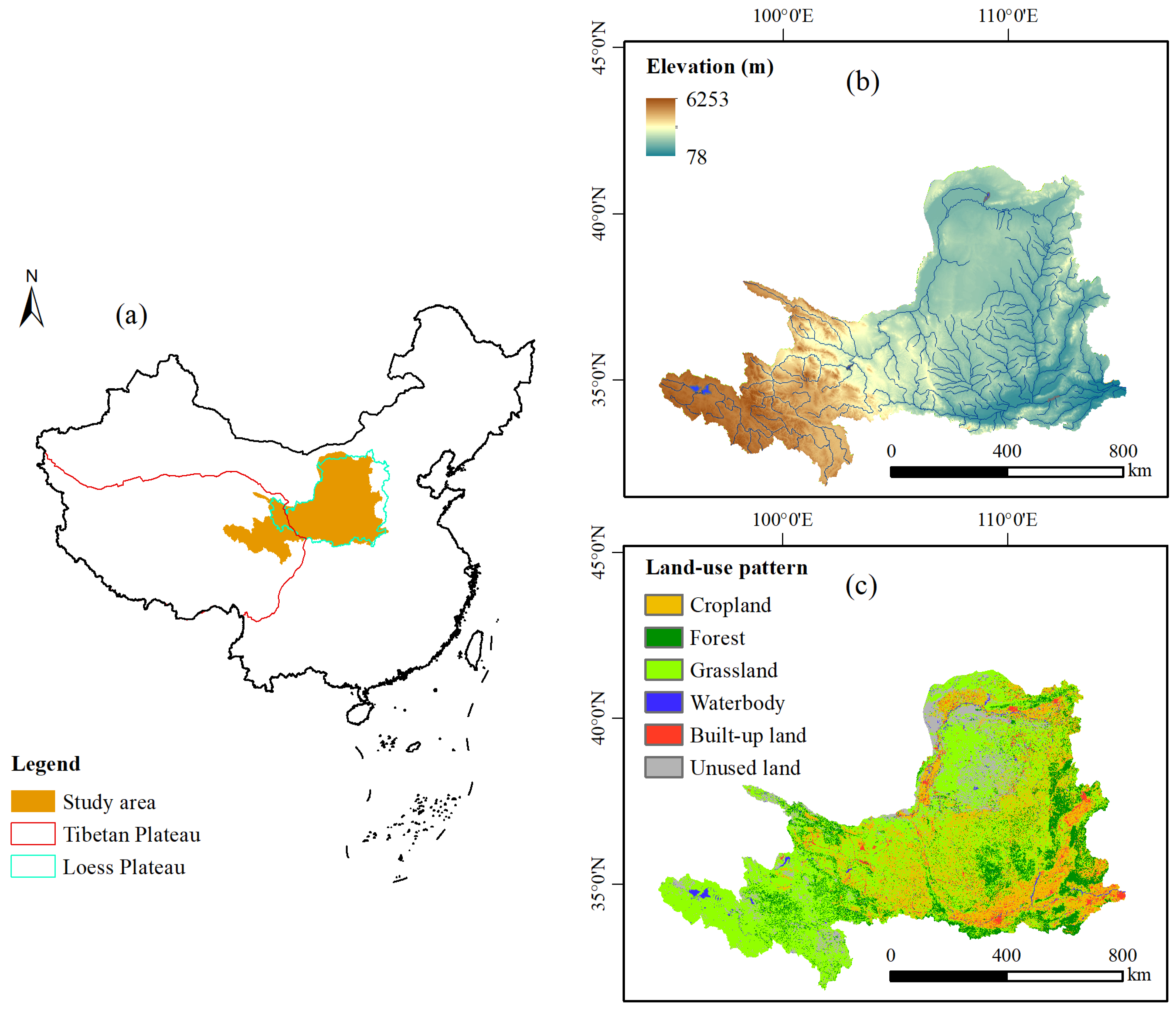
The YRB (32°09′–41°51′ N, 95°52′–119°06′ E) plays a critical role in national efforts for erosion prevention and control [44]. Owing to its complex topography as well as the combined influence of atmospheric and monsoonal circulations, the basin exhibits substantial climatic variability. Annual precipitation ranges from 200 mm to 650 mm across most of the basin, while the southern and lower reaches typically receive more than 650 mm. In contrast, certain inland areas receive less than 200 mm of precipitation annually. The UMYRB covers approximately 7.72 × 10⁵ km², constituting 97.1% of the entire basin’s area. It features pronounced east–west elevation gradients and considerable heterogeneity in geomorphology, climate, water resources, soils, and vegetation (Figure 1). This region is among the most ecologically fragile areas in China. The region is characterized by diverse ecological problems of high severity and frequency, including soil erosion, sandy desertification, grassland degradation, and drought–flood hazards. In recent years, water scarcity and sediment-related challenges have not only severely constrained sustainable economic development within the region but have also posed risks to socioeconomic development and ecological security in downstream areas.

Figure 1. (a) Location of the study area; (b) elevation; (c) land use map for 2020.

2.2. Data Sources

Multiple datasets were used, including land-use, soil, meteorological observations, and remote sensing imagery, as well as county-level vector boundaries (Table S1). Vegetation dynamics were assessed using the MOD13A3 product. The raw MOD13A3 product, provided in HDF format with a sinusoidal projection, was preprocessed using MRT V4.0 software to perform mosaicking, format conversion, and reprojection. Meteorological data were obtained from ground-based stations (Table S2). Since solar radiation observations were not available at meteorological stations, they were assessed using the method proposed by Ma et al. [45]. All meteorological variables were spatially interpolated to 1000 m resolution grids using ArcGIS 10.2. Considering local environmental conditions and prior studies [13], land-use/land-cover (LULC) maps were reclassified into six categories: farmland, grassland, forestland, built-up land, water body, and unused land. All raster datasets were resampled and reprojected to a unified coordinate system (Krasovsky_1940_Albers) with a resolution of 1000 m.

2.3. Methods

2.3.1. Calculation of Soil Conservation Services

SC was assessed using the RUSLE [20,21], expressed as follows:

$$\mathrm{S}\mathrm{C}=\mathrm{R}\times \mathrm{K}\times \mathrm{L}\mathrm{S}\times (1-\mathrm{C}\times \mathrm{P})$$

(1)

where $\mathrm{S}\mathrm{C}$ indicates the soil conservation rate (t·ha⁻¹); $\mathrm{R}$ and $\mathrm{K}$ denote the precipitation erosion factor (MJ·mm·ha⁻¹·h⁻¹) and soil erodibility factor (t·ha·h·ha⁻¹·MJ⁻¹·mm⁻¹), respectively; $\mathrm{L}\mathrm{S}$, $\mathrm{P}$, and $\mathrm{C}$ represent the topographic factor, erosion control practice factor, and vegetation management factor, respectively [46]. Details on parameter localization for RUSLE are provided in Supplementary Tables S3 and S4. Considering the intra-annual variability in rainfall characteristics and vegetation cover, SC was estimated on a seasonal basis and subsequently aggregated to obtain annual values.

2.3.2. Calculation of Landscape Metrics

Landscape metrics were calculated using Fragstats V4.2 software [47] based on LULC maps. In line with previous studies, twenty-four metrics were computed at the landscape and class levels. The selected metrics include percentage of landscape, edge density, largest patch index, mean patch area, mean fractal dimension index, aggregation index, and Shannon’s diversity index (Table S5). At the class level, analyses focused on three dominant land-use categories—farmland, grassland, and forestland—owing to their substantial influence on erosion processes.

2.3.3. Sen’s Slope and Mann–Kendall Method

The Sen’s slope method was used to assess the rate of change in time series data, including soil conservation rate, climatic variables, landscape metrics, and NDVI. The calculation formula is as follows:

$$\mathsf{\beta }=\mathrm{Median}\left({\displaystyle \frac{{\mathrm{x}}_{\mathrm{j}}-{\mathrm{x}}_{\mathrm{i}}}{\mathrm{j}-\mathrm{i}}}\right)$$

(2)

where β denotes the direction and magnitude of change in a variable; x_i and x_j denote the i-th and j-th samples, respectively, with 2000 ≤ i < j ≤ 2020.

The Mann–Kendall trend test method was applied to quantify the statistical significance of trends in the time series [48]. A two-tailed test based on the Z statistic was conducted at a significance level of 0.05.

2.3.4. Stepwise Regression

Stepwise regression was used to identify the factors influencing changes in SC, as it efficiently reduces multicollinearity among the explanatory variables and removes irrelevant variables. The response variable was the SC change rate, while the explanatory variables consisted of the rates of change in climatic factors (precipitation, air temperature, solar radiation, and wind speed), NDVI, landscape metrics, and altitude. The procedure for the stepwise regression analysis was as follows: (1) county-level averages for both response and explanatory variables were calculated using ArcGIS; (2) all variables were standardized using the Z-score method; and (3) stepwise regression analysis was performed in SPSS 20.0, with variable selection based on the criterion of F ≤ 0.05. The analysis was conducted at both seasonal and annual scales.

2.3.5. Geographically Weighted Regression

GWR was applied to investigate the factors influencing changes in SC from the perspective of spatial heterogeneity. The formula is as follows:

$${\mathrm{Y}}_{\mathrm{i}}={\sum }_{\mathrm{j}=1}^{\mathrm{k}}{\mathrm{a}}_{\mathrm{k}}({\mathsf{\mu }}_{\mathrm{i}},{\mathrm{v}}_{\mathrm{i}}){\mathrm{x}}_{\mathrm{ik}}+{{\mathsf{\alpha }}_0\left({\mathsf{\mu }}_{\mathrm{i}},{\mathrm{v}}_{\mathrm{i}}\right)+\mathsf{\epsilon }}_{\mathrm{i}}$$

(3)

where ${\mathrm{Y}}_{\mathrm{i}}$ represents the response variable; $({\mathsf{\mu }}_{\mathrm{i}},{\mathrm{v}}_{\mathrm{i}})$ denotes the geographical coordinates; ${\mathsf{\alpha }}_{\mathrm{k}}({\mathsf{\mu }}_{\mathrm{i}},{\mathrm{v}}_{\mathrm{i}})$ denotes the local regression coefficient for the k-th explanatory variable; ${\mathrm{x}}_{\mathrm{i}\mathrm{k}}$ denotes the independent variables for sample i; ${\mathsf{\alpha }}_0({\mathsf{\mu }}_{\mathrm{i}},{\mathrm{v}}_{\mathrm{i}})$ is the location-specific intercept; ${\mathsf{\epsilon }}_{\mathrm{i}}$ is the random error term. A Gaussian kernel function was used to estimate spatial weights, with an adaptive bandwidth employed for calibration. The optimal bandwidth was determined using the AICc (Akaike Information Criterion). GWR analysis was conducted in ArcGIS 10.2.

3. Results

3.1. Spatiotemporal Variations in Soil Conservation

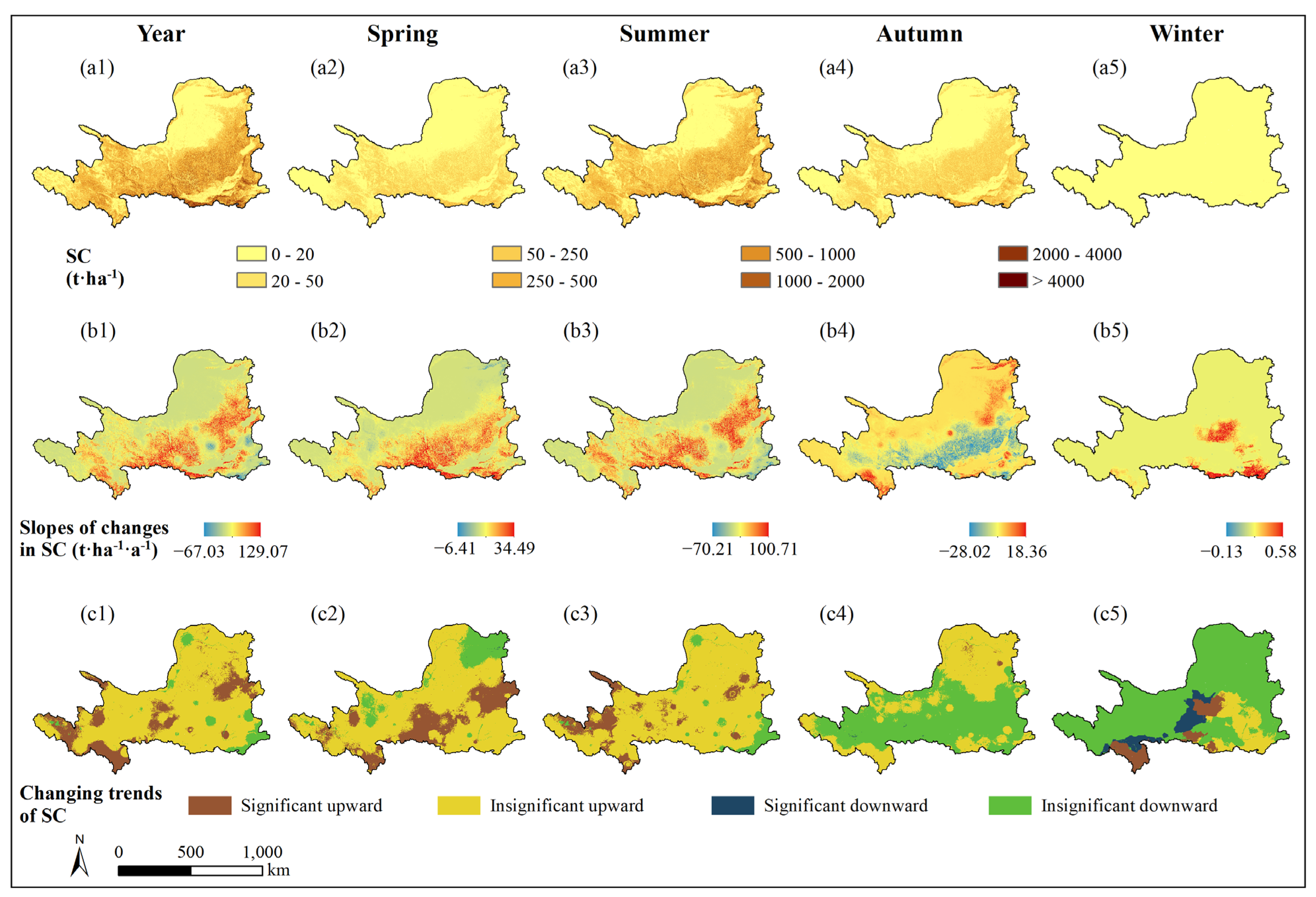
Figure 2 illustrates the spatiotemporal dynamics of SC across the UMYRB. Except for winter, SC demonstrated pronounced spatial heterogeneity. Due to abundant rainfall and dense vegetation, high SC values were mainly found in the southern hilly and mountainous areas. In contrast, the northern region—dominated by deserts and sandy lands—exhibited low SC values, attributable to limited rainfall and sparse vegetation cover. In terms of temporal variation, summer—characterized by concentrated heavy rainfall and vigorous vegetation growth—is the season with the highest SC, whereas spring and autumn displayed comparatively lower SC levels.

Figure 2. Spatial patterns of the average (a1–a5), change rates (b1–b5), and trend classifications (c1–c5) of soil conservation during 2000–2020 at seasonal and annual scales.

The spatial distributions of SC change rates and trends, derived using Sen’s slope and Mann–Kendall trend test method, are shown in Figure 2. The proportions of areas exhibiting different SC change trends are summarized in Table 1. As shown in Figure 2, the spatial patterns of SC change rates and trends varied substantially over the examined time scales. Overall, SC increased over the study period, except during autumn and winter. Specifically, areas exhibiting an increasing SC trend accounted for 88.08% in spring, 93.68% in summer, and 94.30% at the annual scale (Table 1). In contrast, these proportions decreased significantly in autumn (44.75%) and winter (18.95%). The spatial pattern of SC change rates in spring and summer closely resembled the annual pattern, with high-value areas forming a belt-like pattern extending across the central-southern and central-eastern regions (Figure 2). In autumn, regions showing insignificant decreases in SC accounted for 55.19% of the UMYRB, mainly concentrated in the center and south. During winter, the dominant trend in SC was also an insignificant decrease, accounting for 74.57% of the total area, while insignificant increases were mainly observed in the southern peripheral regions and the central part of the UMYRB.

Table 1. Proportions of areas exhibiting different soil conservation change trends across various temporal scales.

Time Scales	Percentage of Areas with Significant Upward (%)	Percentage of Areas with Insignificant Upward (%)	Percentage of Areas with Significant Downward (%)	Percentage of Areas with Insignificant Downward (%)
Annual	17.30	77.00	0.00	5.70
Spring	19.77	68.31	0.04	11.89
Summer	12.09	81.59	0.00	6.31
Autumn	0.55	44.20	0.06	55.19
Winter	7.77	11.18	6.48	74.57

3.2. Driving Forces of Changes in Soil Conservation Based on Stepwise Regression

Table 2 and Table S5 summarize the results of the stepwise regression analysis. All explanatory variables exhibited variance inflation factor values below 7.5 (Table S6), indicating an absence of multicollinearity and redundancy among the explanatory variables. Across all examined time scales, the R² values were high (Table 3), suggesting strong model performance. Compared with climatic variables, landscape metrics were more diverse, but had a relatively weaker influence on SC. Among the climatic variables, precipitation, air temperature, and solar radiation all had positive effects on SC, with precipitation demonstrating a consistently strong influence across all examined time scales. In spring, wind speed emerged as a key driver, exerting a particularly strong negative influence. The drivers of SC change in summer, along with the magnitudes and directions of their effects, closely resembled those at the annual scale. PLAND_1 positively affected SC in spring. PLAND_3 and ED_2 were positively related to SC in summer. In autumn, ED_1 exerted a positive influence on SC, a finding that contrasted with other time scales. Elevation exerted a positive influence on SC throughout the year, particularly in spring and autumn.

Table 2. Stepwise regression results for soil conservation variations at annual and seasonal scales.

Time Scales	Explanatory Variables
	Climatic Factors	Landscape Pattern Factors	Topographical Factor
Annual	Pre (0.746) Tem (0.094)	NDVI (0.158) SHDI (−0.246) ED_1 (−0.126) LPI (−0.117)	Alt (−0.218)
Spring	Pre (0.894) SR (0.169) WS (−0.176)	NDVI (0.132) ED_1 (−0.126) PLAND_1 (0.254) AI_1 (−0.143)	Alt (−0.101)
Summer	Pre (0.810) Tem (0.276) SR (0.145)	PLAND_3 (0.165) NDVI (0.241) LPI_1 (−0.200) ED_1 (−0.147) FRAC_MN_1 (0.095) ED_2 (0.078)
Autumn	Pre (0.822) SR (0.183) Tem (0.084)	ED_1 (0.135) NDVI (−0.110)	Alt (−0.150)

Note: Pre denotes precipitation; SR denotes solar radiation; WS denotes wind speed; Tem denotes air temperature; PLAND denotes percentage of landscape; LPI denotes largest patch index; ED denotes edge density; FRAC_MN denotes mean fractal dimension index; AI denotes aggregation index; SHDI denotes shannon’s diversity index; NDVI denotes normalized difference vegetation index; Alt denotes altitude. For landscape metric_(1, 2, 3), the numbers 1, 2, and 3 represent farmland, forestland, and grassland, respectively.

Table 3. Diagnostic results of the stepwise regression and GWR models.

Time Scales	AICc		R2		Adjusted R2		Residuals’ Moran’s I
	Stepwise Regression	GWR	Stepwise Regression	GWR	Stepwise Regression	GWR	Stepwise Regression	GWR
Annual	568.200	452.916	0.638	0.899	0.629	0.833	0.155 (0.000)	0.025 (0.250)
Spring	483.657	257.734	0.728	0.933	0.721	0.901	0.166 (0.000)	0.035 (0.117)
Summer	516.895	422.421	0.698	0.862	0.689	0.814	0.250 (0.000)	0.022 (0.312)
Autumn	533.956	309.867	0.674	0.923	0.667	0.884	0.349 (0.000)	0.004 (0.780)

Note: AICc denotes Akaike’s Information Criterion; the numbers in brackets represent the p-value of global Moran’s I.

The results of the model diagnostics for the stepwise regression and GWR are presented in Table 3. The diagnostic parameters include Akaike’s Information Criterion (AICc), global Moran’s I, and Adjusted R². Moran’s I was employed to evaluate the extent of spatial autocorrelation in the model residuals. Compared with stepwise regression, GWR exhibited a lower AICc and a higher Adjusted R² value, indicating a substantial improvement in its ability to explain the relationships between the influencing factors and SC changes. The Moran’s I values for the GWR residuals were lower than those for stepwise regression and were not statistically significant, suggesting that the GWR residuals were randomly distributed in space. Therefore, the GWR approach was more robust and demonstrated superior performance compared to the stepwise regression method.

3.3. Driving Forces of Changes in Soil Conservation Based on GWR Method

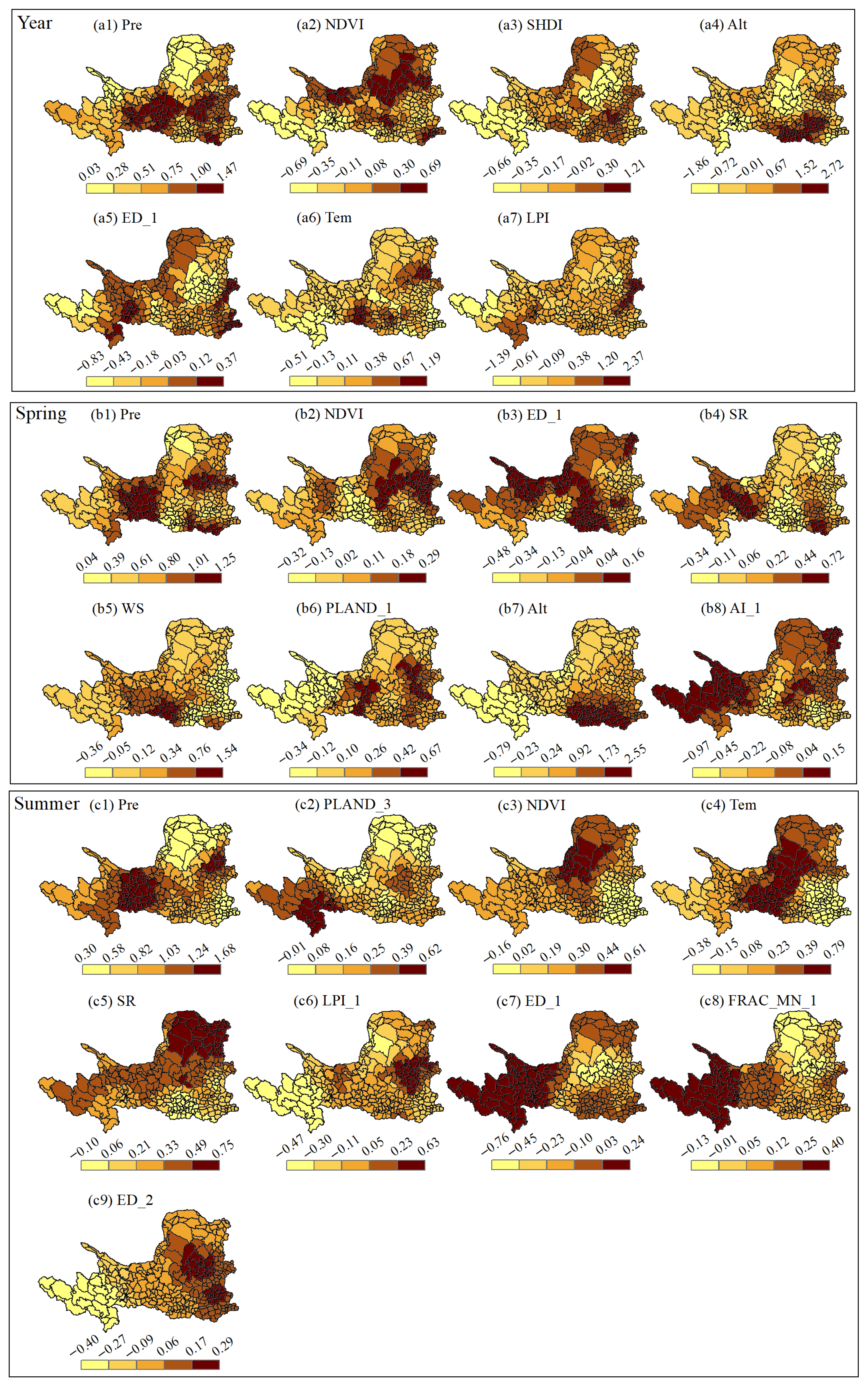
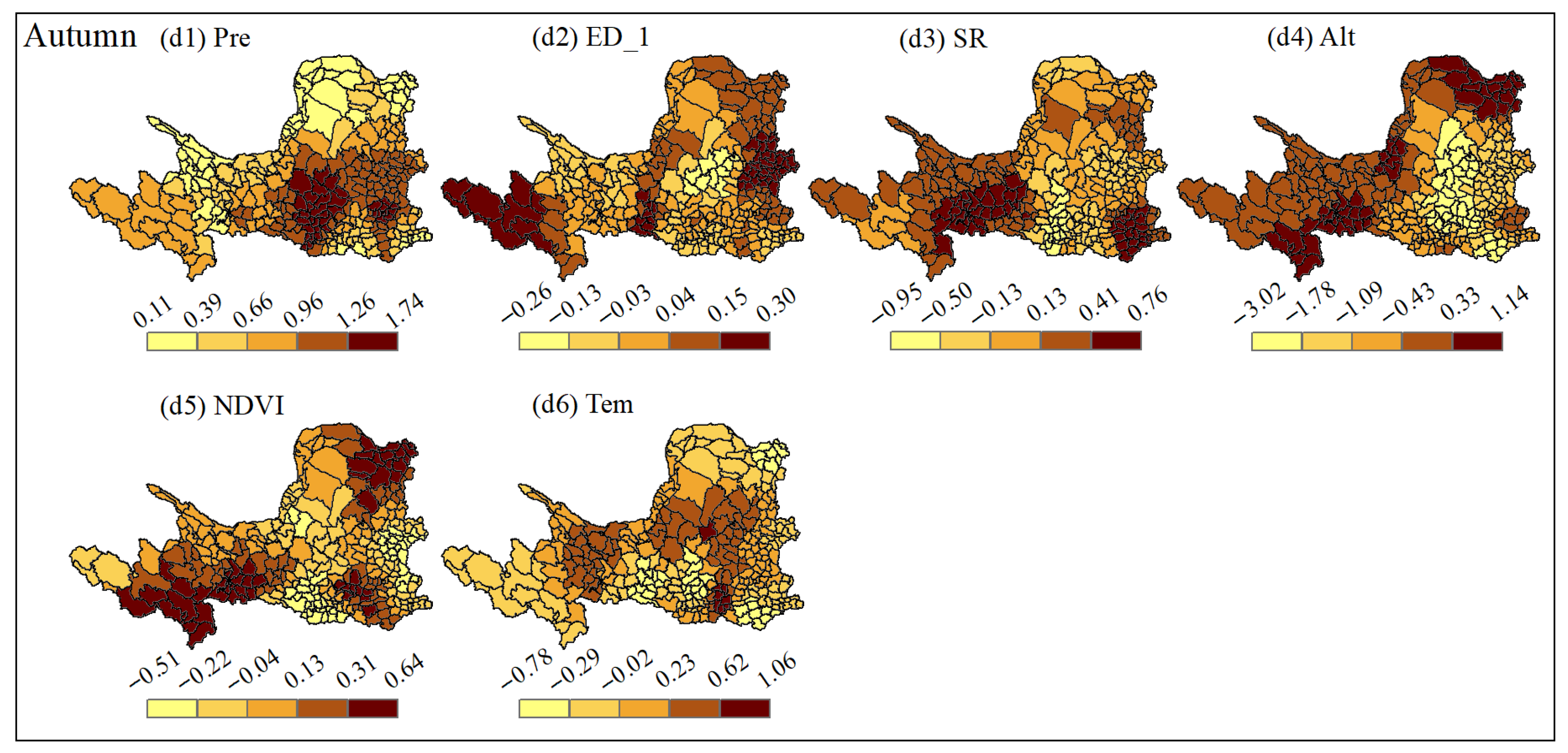
The estimated regression coefficients derived from the GWR models are presented in Figure 3. At the annual scale, the estimated regression coefficients for precipitation varied between 0.03 and 1.47, displaying a spatial pattern characterized by lower coefficients in the north and higher ones in the center and south. The effect of NDVI on SC exhibited a clear north–south gradient, transitioning from positive in the north to negative in the south. The spatial patterns of the impacts of SHDI and ED_1 on SC were broadly similar, with high-impact zones primarily located in the northwest and southeast. For altitude, higher regression coefficients were observed in the southeastern and central regions; notably, altitude contributed positively to SC in the southeast but had a suppressive effect in the central region. Temperature generally exerted a positive influence on SC, with areas of stronger impact primarily distributed in the northeast and central–south. The effect of LPI on SC was predominantly positive, displaying a fragmented pattern, with high-value areas mainly distributed along the eastern and southwestern margins.

Figure 3. Spatial variation of regression coefficients from the GWR model, illustrating the relationships between soil conservation changes and driving factors across different time scales. Pre denotes precipitation; SR denotes solar radiation; WS denotes wind speed; Tem denotes air temperature; PLAND denotes percentage of landscape; LPI denotes largest patch index; ED denotes edge density; FRAC_MN denotes mean fractal dimension index; AI denotes aggregation index; SHDI denotes shannon’s diversity index; NDVI denotes normalized difference vegetation index; Alt denotes altitude. For landscape pattern metric (1, 2, 3), the numbers 1, 2, and 3 represent farmland, forestland, and grassland, respectively.

In spring, the estimated regression coefficients for precipitation varied between 0.04 and 1.25, with higher values primarily concentrated in the center and west. NDVI exerted a stronger influence in the central region and a weaker influence in the surrounding areas. Specifically, NDVI had a positive effect on SC in the central-northern and northern regions, while negative effects were more prevalent in the central-western region. ED_1 exerted a predominantly negative influence on SC, with positive effects observed in the northwestern and central-southern regions. Solar radiation generally had a positive effect on SC, with stronger effects concentrated in the central-western and southeastern regions. Wind speed exerted a predominantly positive effect, with high-value areas distributed along the southwestern edge. Notably, the impact of PLAND_1 and precipitation on soil conservation was spatially similar. The impact of altitude on SC was mainly positive, exhibiting a decreasing trend from south to north. AI_1 primarily exerted a suppressive effect on SC.

In summer, higher precipitation coefficients were primarily concentrated in the northeastern and central-western regions. PLAND_3 exerted a largely positive effect on SC, with higher coefficients observed in the western region and comparatively lower values in the east. Both NDVI and temperature had a positive influence on SC, exhibiting comparable spatial distributions, with stronger effects predominantly concentrated in the center and west. The impact of solar radiation on SC showed a spatial pattern with stronger effects in the south and weaker ones in the north. The influence of LPI_1 on SC displayed clear spatial variation, being positive in the east but negative in the west. FRAC_MN_1 was generally positively associated with SC, with a spatial distribution closely resembling that of ED_1. ED_2 had a negative effect in the west and a positive effect in the east.

In autumn, the regression coefficients for precipitation ranged from 0.11 to 1.74, with higher values concentrated in the center and south. ED_1 exhibited a distinct spatial influence on SC: positive at the western and eastern margins, but negative in the central area. Solar radiation and NDVI exhibited similar spatial patterns in their influence on SC, with positive effects clustered in the southwestern, northeastern, and southeastern regions. Altitude predominantly exerted a negative influence on SC. The effect of air temperature on SC decreased radially from the center towards the periphery.

4. Discussion

4.1. Impacts of Climate Variability on Soil Conservation

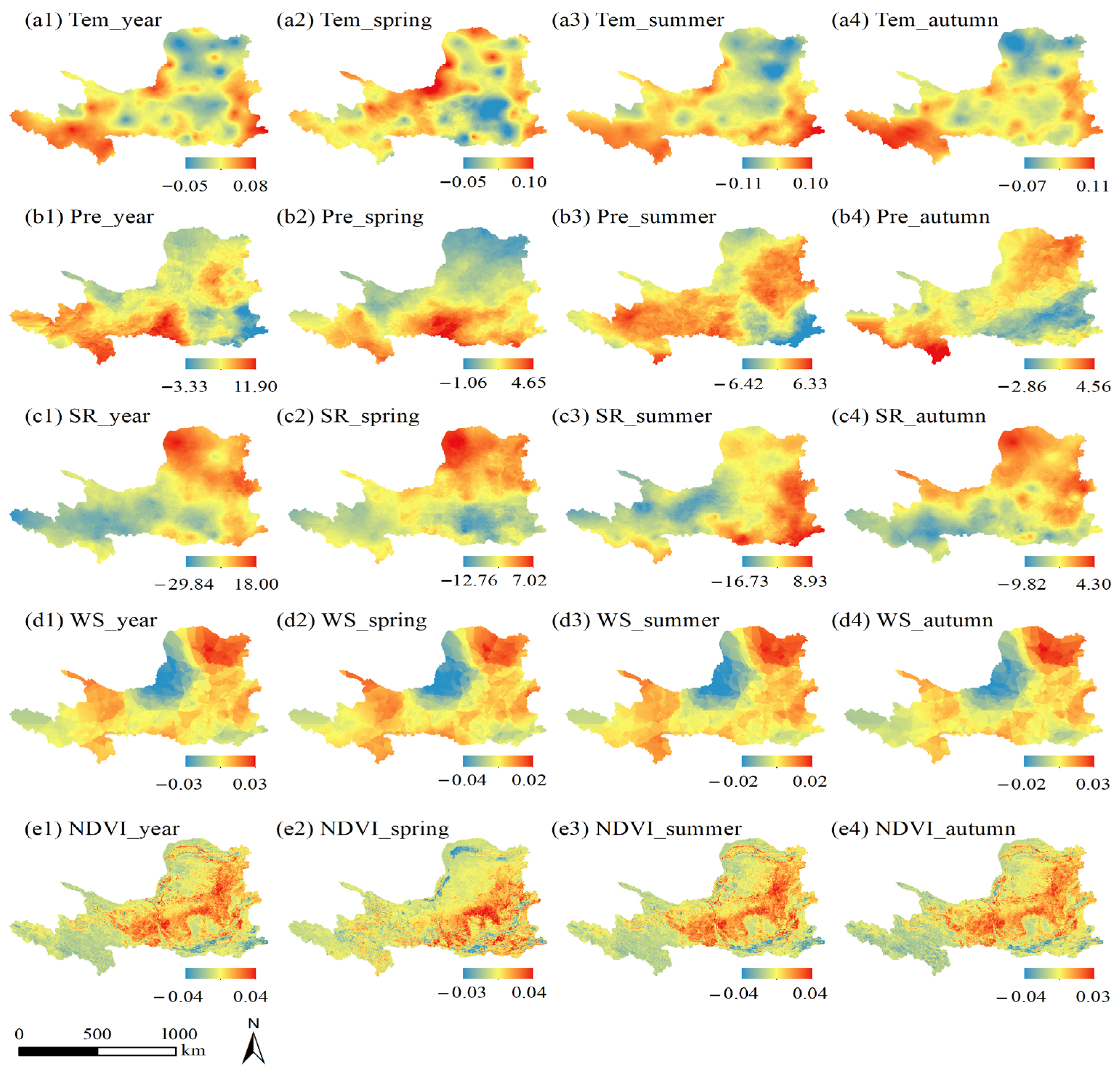
Climatic factors commonly influence SC through both direct and indirect pathways [11]. From 2000 to 2020, the UMYRB experienced notable climatic changes, including increases in temperature and precipitation, a decline in solar radiation and an overall increase in wind speed (Figure 4; Table S7). Seasonal and annual climate variations exhibited pronounced spatial heterogeneity (Figure 4), leading to spatial and temporal variability in SC (Figure 3). Of the examined climatic variables, precipitation had the most dominant and consistently positive influence on SC across all examined time scales (Figure 3; Table 2). This influence can be attributed to two primary factors. First, although total precipitation increased across most of the UMYRB (Table S7), erosive precipitation—defined as rainfall events with sufficient intensity, duration, or kinetic energy to detach soil particles and initiate or accelerate soil erosion—declined following the implementation of large-scale vegetation restoration projects [49]. Second, given that vegetation growth in the UMYRB is highly dependent on water availability [50], precipitation is the primary water source. The observed increase in precipitation alleviated soil moisture stress, promoted vegetation growth, and ultimately enhanced SC capacity [24]. As shown in Figure 3, the correlation coefficient between precipitation and SC was highest in the central and southern parts of the UMYRB, where the extensive forest and grassland cover exhibited heightened sensitivity to precipitation variability. Consistent with Guo et al. [8], air temperature had both positive and negative influences on SC (Figure 3). This dual effect is explained by two main mechanisms. On the one hand, rising temperatures can facilitate vegetation growth under adequate water availability [51], thereby enhancing SC. On the other hand, elevated temperatures may increase plant transpiration and surface evaporation, resulting in soil moisture depletion that suppresses vegetation growth and limits improvements in SC. This dual effect is supported by a previous study which found that there is a threshold in vegetation’s response to temperature changes [52,53]. A negative correlation was observed between wind speed and SC in spring (Table 2), which can be attributed to two primary mechanisms. First, strong winds in spring act as a major agent in shaping geomorphic processes, including the erosion of surface rocks and soils through deflation and abrasion. Wind-driven transport facilitates the long-distance movement of sedimentary particles, which eventually settle and form important sources for soil erosion [54]. Second, higher wind speeds can intensify raindrop energy and velocity, exacerbating their impact on the soil surface and promoting soil disaggregation and particle detachment, which ultimately increases the risk of water erosion [55].

Figure 4. Slopes of changes in climatic factors and NDVI at seasonal and annual scales over the period 2000–2020. Units: Temperature (Tem, °C), Precipitation (Pre, mm), Solar radiation (SR, MJ·m⁻²), Wind speed (WS, m·s⁻¹).

4.2. Impacts of Changes in Landscape Patterns on Soil Conservation

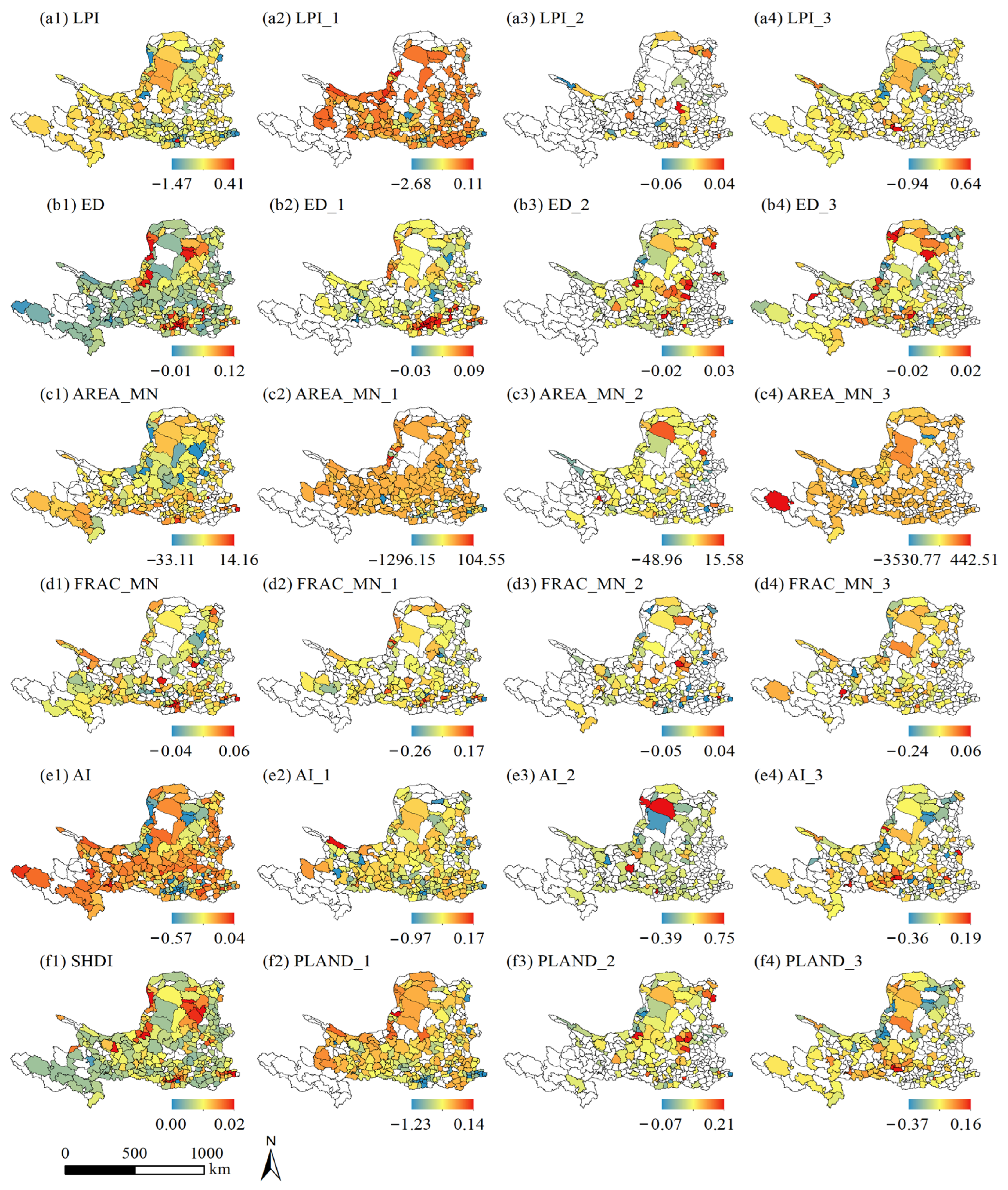
Landscape metrics are employed for the quantitative analysis of landscape composition and configuration [47]. As shown in Figure 5, changes in landscape metrics exhibited pronounced spatial heterogeneity. At the landscape level, LPI, AREA_MN, and AI predominantly showed decreasing trends in most of the counties, whereas ED and SHDI displayed increasing trends, indicating a shift toward more diversified, fragmented, and dispersed landscape patterns. In comparison with landscape composition metrics, landscape configuration metrics exerted a stronger influence on SC (Table 2). The edge density of forestland (ED_2) promoted SC, whereas the aggregation index of farmland (AI_1) inhibited it, which aligns with the results reported by Dai et al. [21]. Landscape patch boundaries act as intermediaries for surface water movement, soil deposition, and nutrient exchange [56,57]. Increased fragmentation of landscape patches enhances surface roughness and flow resistance, thereby reducing runoff velocity and facilitating improved water infiltration into the soil. Ultimately, these processes mitigate soil erosion and sediment transport, thereby enhancing SC capacity.

Figure 5. Slopes of changes in landscape metrics at the county scale during 2000–2020. PLAND denotes percentage of landscape; LPI denotes largest patch index; ED denotes edge density; FRAC_MN denotes mean fractal dimension index; AI denotes aggregation index; SHDI denotes shannon’s diversity index. To enhance the intuitiveness of the results, the value of FRAC_MN was amplified by 100 times. The white areas indicate that the change rate of the landscape metric is 0. For landscape metric (1, 2, 3), the numbers 1, 2, and 3 represent farmland, forestland, and grassland, respectively.

Regarding landscape composition metrics, variations in landscape composition can substantially alter soil properties and community structures, thereby affecting SC dynamics [57]. Among these metrics, farmland expansion—as indicated by increases in PLAND_1—promoted SC in spring, consistent with prior findings from other semi-arid environments of northern China [58]. The enlargement of farmland patches was accompanied by improved agricultural management efficiency, while concurrent advancements in land management practices increased soil infiltration, strengthened drainage, and promoted vegetation cover [59]. Together, these factors enhanced the SC capacity of farmlands. Moreover, ecological restoration projects have resulted in a substantial amount of unused land being converted into grassland or forest in the middle YRB [41]. Compared with forests and farmlands, grasslands require less water for growth, resulting in higher survival rates under semi-arid restoration conditions [60,61]. Grassland expansion was positively correlated with improvements in SC (Table 2), which is consistent with previous findings [62]. The enhancement of SC in grasslands can largely be attributed to their ecohydrological advantages, which operate through two primary mechanisms: (1) reduced evapotranspiration demand under water-limited conditions, thereby minimizing soil moisture depletion in semi-arid environments; and (2) dense root networks that promote soil aggregation and increases erosion resistance through biomechanical reinforcement. Thus, grasslands play a critical role in reconciling restoration effectiveness with water resource constraints in regions susceptible to aridification.

From 2000 to 2020, NDVI increased across most (>85%) of the UMYRB (Figure 4; Table S7), with declines primarily concentrated along the western, northern, and southeastern margins. NDVI generally had a positive influence on SC. This positive effect is likely attributable to the following mechanisms: increased vegetation cover enhances the interception of rainfall by the canopy, reducing the kinetic energy and impact velocity of raindrops. This process improves surface water infiltration and decreases runoff energy, thereby lowering sediment transport [25,63]. Additionally, plant root systems stabilize soil structure by anchoring soil particles, thereby increasing resistance to erosion. Collectively, these biophysical processes underpin the enhancement of SC capacity.

At local scales, topographic factors predominantly regulate hydrothermal conditions, thereby influencing soil erosion processes [64]. In the UMYRB, SC exhibited a decreasing trend with increasing altitude (Figure 3; Table 2), driven by two primary mechanisms. First, high-altitude zones, mainly located in the upper YRB, are characterized by steep slopes (Figure 1). Steeper slopes tend to intensify surface runoff and sediment transport potential, thus reducing SC capacity. Second, low-altitude areas that serve as primary regions for agricultural activities, have been the focus of the Grain-for-Green Program, which has converted sloped farmland and unused land into grassland or forest [24,41]. These ecological restoration initiatives have effectively mitigated soil erosion and enhanced SC in these areas.

4.3. Implications for Ecosystem Management

This study presents two key innovations. First, the integration of stepwise regression with GWR allows for a more nuanced analysis of the spatial non-stationarity in the relationships between driving factors and SC, thereby providing a stronger basis for developing site-specific soil and water conservation strategies. Second, in contrast to previous studies limited to annual-scale analyses, this study reveals seasonal variations in the relationships between SC and its drivers across the UMYRB (Figure 3; Table 2). These findings underscore the necessity of formulating season-specific soil and water conservation strategies.

In spring, strong winds, occasional extreme rainfall events, and limited vegetation cover increase the risk of wind and water erosion, necessitating targeted erosion-control measures. For instance, applying straw mulch during the regreening period—when crop cover is sparse—can effectively reduce surface erosion [65]. Grazing should be strictly prohibited during this period, and planting shrubs or herbaceous species in forested areas may further mitigate erosion. Additionally, farmland expansion contributes to increased SC during spring. Given the critical role of farmland in sustaining local livelihoods and the necessity for SC improvement, large farmland plots should be subdivided into smaller patches. Conservation tillage practices, such as stubble retention, straw mulching, and raised-bed planting, should be promoted to minimize soil and water loss. Summer, characterized by abundant rainfall and vigorous vegetation growth, faces the greatest risk of water erosion in the UMYRB [66], making it a critical period for implementing SC measures (Figure S1). In fragile mountainous regions where precipitation strongly influences SC, erosion control strategies such as gully stabilization and adjustments in cultivation methods are recommended [67]. Converting unused land or marginally arable land into grassland is recommended to enhance landscape stability and promote sustainable land use. During this season, changes in SC were positively associated with the largest patch index of grasslands (Table 2). Therefore, land-use conversions involving grasslands should be carefully regulated in erosion-prone regions, and overgrazing should be prohibited to preserve their erosion-buffering functions.

Beyond seasonal dynamics, certain environmental variables also require targeted policy interventions. The positive effect of NDVI on SC underscores the importance of maintaining and further enhancing vegetation restoration initiatives. To balance vegetation recovery with hydrological processes and promote long-term ecological resilience and sustainability, restoration measures should be tailored to local environmental conditions [68]. Restoration efforts should prioritize native species, supported by natural regeneration and site-specific interventions. Moreover, given the negative influence of altitude on SC, it is essential to implement erosion control measures in high-altitude and steeply sloped areas, which should be actively vegetated. Although these recommendations provide a scientific basis for improving SC, their effective implementation requires coordinated efforts from multiple government agencies and stakeholders of each county.

4.4. Limitations and Future Directions

Despite the valuable insights gained, several limitations must be recognized. The inherent limitations of the RUSLE, together with uncertainties in its input parameters, may reduce the accuracy of SC estimates [69]. Specifically, the RUSLE was originally developed to estimate rill and sheet erosion, without accounting for gully, gravity, or streambank erosion [70]. To more accurately represent the processes of sediment detachment, transport, and deposition, future research should integrate RUSLE with process-based soil erosion models. Additionally, future studies could improve the characterization of the C factor by using hyperspectral and microwave remote sensing technology to account for the crucial role of non-photosynthetic vegetation in mitigating soil erosion [71]. Moreover, due to the difficulty of accurately estimating the P factor at large spatial scales, it is often approximated in modeling, potentially leading to biased estimates [72]. Nonetheless, this study primarily aimed to uncover the spatio-temporal dynamics of SC, rather than to quantify its absolute value. Future efforts should focus on refining the RUSLE by incorporating localized parameters derived from field investigations and observations, thereby enhancing its accuracy and applicability for SC assessments. Methodologically, both stepwise regression and GWR are based on linear assumptions, whereas the relationships between soil erosion and its driving factors are likely non-linear [73]. Climatic and landscape pattern factors frequently interact and are mutually dependent [74], complicating the disentanglement of their individual contributions. Therefore, future studies should prioritize multivariate non-linear statistical approaches to better capture the complex causal pathways—including both direct and indirect effects—by which interacting drivers influence SC dynamics. Finally, this study focused solely on water erosion suppression. However, in the UMYRB, the co-occurrence or alternation of wind and water erosion results in a compound geomorphic process—complex erosion by wind and water—which is a primary driver of land degradation in drylands. Further research is needed to clarify the mechanisms underlying this type of erosion and to develop regionally adapted control strategies.

5. Conclusions

Considering the intra-annual variability in rainfall characteristics and vegetation cover, this study used the RUSLE to quantitatively assess SC in the UMYRB over the past 21 years at both seasonal and annual scales. Stepwise regression and GWR were used to identify the driving factors shaping the spatio-temporal dynamics of SC. The results revealed that SC provision varied markedly across seasons, with significantly higher values observed in summer than in other seasons. Spatially, SC was lower in the arid northern zones and higher in the mountainous southern regions, primarily influenced by variations in precipitation, topography, and vegetation cover. From 2000 to 2020, SC generally increased throughout the year, particularly in spring and summer, while decreasing trends were observed in autumn and winter. Stepwise regression and GWR analyses identified that precipitation and NDVI were the dominant drivers of SC, with their effects varying seasonally and exhibiting pronounced spatial heterogeneity. Expanding the area of appropriate forest stands and subdividing large farmland and grassland areas into smaller patches would be beneficial for enhancing SC. These findings underscore the necessity of integrating time-scale effects of driving factors into the development of soil and water conservation strategies, particularly in erosion-prone watersheds with substantial seasonal climatic differences. By combining stepwise regression and GWR, this study offers a robust analytical framework for examining spatially non-stationary relationships between SC and its driving factors, thereby supporting ecosystem management.

References

- Yang, J.; Badreldin, N.; Gao, Y.; Yan, C.; Zhao, Y.; Dyck, M.; He, H. Innovative methods for monitoring soil erosion: Utilizing InSAR technology effectively. Catena 2025, 261, 109547. [Google Scholar] [CrossRef]
- Borrelli, P.; Robinson, D.; Panagos, P.; Lugato, E.; Yang, J.; Alewell, C.; Wuepper, D.; Montanarella, L.; Ballabio, C. Land use and climate change impacts on global soil erosion by water (2015–2070). Proc. Natl. Acad. Sci. USA 2020, 117, 21994–22001. [Google Scholar] [CrossRef]
- Khosravi, K.; Rezaie, F.; Cooper, J.; Kalantari, Z.; Abolfathi, S.; Hatamiafkoueieh, J. Soil water erosion susceptibility assessment using deep learning algorithms. J. Hydrol. 2023, 618, 129229. [Google Scholar] [CrossRef]
- Firoozi, A.; Firoozi, A. Water erosion processes: Mechanisms, impact, and management strategies. Results Eng. 2024, 24, 103237. [Google Scholar] [CrossRef]
- Tuo, M.; Qiao, H.; Xu, G.; Wang, B.; Wan, S.; Wang, X.; Xie, X. Effects of vegetation types on hillslope runoff and soil erosion on the Loess Plateau. Catena 2025, 260, 109487. [Google Scholar] [CrossRef]
- Liu, Y.; Zhao, W.; Jia, L. Soil conservation service: Concept, assessment, and outlook. Acta Ecol. Sin. 2019, 39, 432–440. [Google Scholar] [CrossRef]
- An, Y.; Zhao, W.; Li, C.; Ferreira, C. Temporal changes on soil conservation services in large basins across the world. Catena 2022, 209, 105793. [Google Scholar] [CrossRef]
- Guo, Y.; Peng, C.; Zhu, Q.; Wang, M.; Wang, H.; Peng, S.; He, H. Modelling the impacts of climate and land use changes on soil water erosion: Model applications, limitations and future challenges. J. Environ. Manag. 2019, 250, 109403. [Google Scholar] [CrossRef]
- IPCC. AR6 Synthesis Report: Climate Change 2023. Available online: https://www.ipcc.ch/report/sixth-assessment-report-cycle/ (accessed on 15 September 2025).
- Wu, H.; Su, X.; Singh, V. Increasing risks of future compound climate extremes with warming over global land masses. Earth’s Future 2023, 11, e2022EF003466. [Google Scholar] [CrossRef]
- Li, Z.; Fang, H. Impacts of climate change on water erosion: A review. Earth-Sci. Rev. 2016, 163, 94–117. [Google Scholar] [CrossRef]
- Eekhout, J.; de Vente, J. Global impact of climate change on soil erosion and potential for adaptation through soil conservation. Earth-Sci. Rev. 2022, 226, 103921. [Google Scholar] [CrossRef]
- Liu, J.; Ning, J.; Kuang, W.; Xu, X.; Zhang, S.; Yan, C.; Li, R.; Wu, S.; Hu, Y.; Du, G.; et al. Spatio-temporal patterns and characteristics of land-use change in China during 2010–2015. Acta Geogr. Sin. 2018, 73, 789–802. [Google Scholar] [CrossRef]
- He, C.; Zhang, J.; Liu, Z.; Huang, Q. Characteristics and progress of land use/cover change research during 1990-2018. J. Geogr. Sci. 2022, 32, 537–559. [Google Scholar] [CrossRef]
- Chen, C.; Zhao, G.; Zhang, Y.; Bai, Y.; Tian, P.; Mu, X.; Tian, X. Linkages between soil erosion and long-term changes of landscape pattern in a small watershed on the Chinese Loess Plateau. Catena 2023, 220, 106659. [Google Scholar] [CrossRef]
- Zhou, P.; Tian, Y.; Zhai, J.; Song, X.; Li, Y.; Sun, W. How does land use transfer affect ecosystem services in Northwest China? Ecol. Eng. 2025, 219, 107712. [Google Scholar] [CrossRef]
- Xue, S.; Ma, B.; Wang, C.; Li, Z. Identifying key landscape pattern indices influencing the NPP: A case study of the upper and middle reaches of the Yellow River. Ecol. Model. 2023, 484, 110457. [Google Scholar] [CrossRef]
- Xia, H.; Kong, W.; Zhou, G.; Sun, O. Impacts of landscape patterns on water-related ecosystem services under natural restoration in Liaohe River Reserve, China. Sci. Total Environ. 2021, 792, 148290. [Google Scholar] [CrossRef]
- Song, S.; Yu, D.; Li, X. Impacts of changes in climate and landscape pattern on soil conservation services in a dryland landscape. Catena 2023, 222, 106869. [Google Scholar] [CrossRef]
- Tang, Z.; Li, R. Small watersheds are the best control and management unit for improving soil conservation services in karst areas. Sci. Total Environ. 2024, 953, 176162. [Google Scholar] [CrossRef]
- Dai, E.; Lu, R.; Yin, J. Identifying the effects of landscape pattern on soil conservation services on the Qinghai-Tibet Plateau. Glob. Ecol. Conserv. 2024, 50, e02850. [Google Scholar] [CrossRef]
- Yang, Z.; Gu, T.; Zeng, Y.; Chen, W.; Zhang, X.; Pan, S. Spatially non-stationary relationships between landscape fragmentation and soil conservation services in China, 2000–2018. Ecol. Indic. 2024, 160, 111913. [Google Scholar] [CrossRef]
- Qiu, J.; Carpenter, S.; Booth, E.; Motew, M.; Zipper, S.; Kucharik, C.; Loheide II, S.; Turner, M. Understanding relationships among ecosystem services across spatial scales and over time. Environ. Res. Lett. 2018, 13, 054020. [Google Scholar] [CrossRef]
- Chen, J.; Chen, Y.; Wang, K.; Zhang, H.; Tian, H.; Cao, J. Impacts of land use, rainfall, and temperature on soil conservation in the Loess Plateau of China. Catena 2024, 239, 107883. [Google Scholar] [CrossRef]
- Hao, R.; Yu, D.; Liu, Y.; Liu, Y.; Qiao, J.; Wang, X.; Du, J. Impacts of changes in climate and landscape pattern on ecosystem services. Sci. Total Environ. 2017, 579, 718–728. [Google Scholar] [CrossRef]
- Cao, Y.; Hua, L.; Tang, Q.; Liu, L.; Cai, C. Evaluation of monthly-scale soil erosion spatio-temporal dynamics and identification of their driving factors in Northeast China. Ecol. Indic. 2023, 150, 110187. [Google Scholar] [CrossRef]
- Sánchez-Canales, M.; López-Benito, A.; Acuña, V.; Ziv, G.; Hamel, P.; Chaplin-Kramer, R.; Elorza, F. Sensitivity analysis of a sediment dynamics model applied in a Mediterranean river basin: Global change and management implications. Sci. Total Environ. 2015, 502, 602–610. [Google Scholar] [CrossRef] [PubMed]
- Bai, Y.; Ochuodho, T.; Yang, J. Impact of land use and climate change on water-related ecosystem services in Kentucky, USA. Ecol. Indic. 2019, 102, 51–64. [Google Scholar] [CrossRef]
- Xiao, S.; Xia, H.; Zhai, J.; Jin, D.; Gao, H. Trade-off and synergy relationships and driving factor analysis of ecosystem services in the Hexi Region. Remote Sens. 2024, 16, 3147. [Google Scholar] [CrossRef]
- Punzo, G.; Castellano, R.; Bruno, E. Using geographically weighted regressions to explore spatial heterogeneity of land use influencing factors in Campania (Southern Italy). Land Use Policy 2022, 112, 105853. [Google Scholar] [CrossRef]
- Li, Y.; Zhen, W.; Shi, D.; Tang, Y.; Xia, B. Coupling coordination and influencing mechanism of ecosystem services using remote sensing: A case study of food provision and soil conservation. Remote Sens. 2024, 16, 4598. [Google Scholar] [CrossRef]
- Liang, F.; Zhu, R.; Lin, S. Exploring spatial relationship between landscape configuration and ecosystem services: A case study of Xiamen–Zhangzhou–Quanzhou in China. Ecol. Model. 2023, 486, 110527. [Google Scholar] [CrossRef]
- Wang, K.; Zhou, J.; Tan, M.; Lu, P.; Xue, Z.; Liu, M.; Wang, X. Impacts of vegetation restoration on soil erosion in the Yellow River Basin, China. Catena 2024, 234, 107547. [Google Scholar] [CrossRef]
- Wu, Q.; Jiang, X.; Shi, X.; Zhang, Y.; Liu, Y.; Cai, W. Spatiotemporal evolution characteristics of soil erosion and its driving mechanisms-a case Study: Loess Plateau, China. Catena 2024, 242, 108075. [Google Scholar] [CrossRef]
- Fu, B.; Wu, X.; Wang, Z.; Wu, X.; Wang, S. Coupling human and natural systems for sustainability: Experience from China’s Loess Plateau. Earth Syst. Dynam. 2022, 13, 795–808. [Google Scholar] [CrossRef]
- Li, H.; Guan, Q.; Sun, Y.; Wang, Q.; Liang, L.; Ma, Y.; Du, Q. Spatiotemporal analysis of the quantitative attribution of soil water erosion in the upper reaches of the Yellow River Basin based on the RUSLE-TLSD model. Catena 2022, 212, 106081. [Google Scholar] [CrossRef]
- Tian, S.; Xu, M.; Jiang, E.; Wang, G.; Hu, H.; Liu, X. Temporal variations of runoff and sediment load in the upper Yellow River, China. J. Hydrol. 2019, 568, 46–56. [Google Scholar] [CrossRef]
- Li, Y.; Li, R.; Zhou, T.; Sun, J.; He, Y.; Lan, X.; Chen, Z. Pattern and dynamics of ecological vulnerability in the upper reach of Yellow River. J. Mt. Sci. 2025, 22, 2177–2190. [Google Scholar] [CrossRef]
- Tian, X.; Zhao, G.; Mu, X.; Zhang, P.; Gao, P.; Sun, W.; Lu, X.; Tian, P. Decoupling effects of driving factors on sediment yield in the Chinese Loess Plateau. Int. Soil Water Conserv. Res. 2023, 11, 60–74. [Google Scholar] [CrossRef]
- Zhang, J.; Li, J.; Yu, H. Dynamic changes and distribution characteristics of soil and water loss in Loess Plateau area of Yellow River Basin. Res. Soil Water Conserv. 2025, 32, 110–116. [Google Scholar] [CrossRef]
- Liu, X.; Li, X.; Jiang, D. Landscape pattern identification and ecological risk assessment using land-use change in the Yellow River Basin. Trans. Chin. Soc. Agric. Eng. 2021, 37, 265–274. [Google Scholar] [CrossRef]
- Mitchell, M.; Suarez-Castro, A.; Martinez-Harms, M.; Maron, M.; McAlpine, C.; Gaston, K.; Johansen, K.; Rhodes, J. Reframing landscape fragmentation’s effects on ecosystem services. Trends Ecol. Evol. 2015, 30, 190–198. [Google Scholar] [CrossRef]
- Li, W.; Kang, J.; Wang, Y. Seasonal changes in ecosystem health and their spatial relationship with landscape structure in China’s Loess plateau. Ecol. Indic. 2024, 163, 112127. [Google Scholar] [CrossRef]
- Liu, Q.; Qiao, J.; Li, M.; Huang, M. Spatiotemporal heterogeneity of ecosystem service interactions and their drivers at different spatial scales in the Yellow River Basin. Sci. Total Environ. 2024, 908, 168486. [Google Scholar] [CrossRef]
- Ma, Y.; Li, X.; Song, J.; Gao, C.; Zhao, D.; Shen, Y. The climatological calculation of global solar radiation and its temporal and spatial distribution in Inner Mongolia Autonomous Region. J. Meteorol. Environ. 2013, 29, 102–109. [Google Scholar]
- Renard, K.; Foster, G.; Weesies, G.; McCool, D.; Yoder, D. Predicting Soil Erosion by Water: A Guide to Conservation Planning with the Revised Universal Soil Loss Equation (RUSLE); Agricultural Handbook: No. 703; USDA: Washington, DC, USA, 1997.
- McGarigal, K.; Cushman, S.; Ene, E. FRAGSTATS v4: Spatial Pattern Analysis Program for Categorical Maps. Computer Software Program Produced by the Authors. Available online: https://www.fragstats.org (accessed on 17 September 2025).
- Cano, D.; Cacciuttolo, C.; Rosario, C.; Barzola, R.; Pizarro, S.; Ramirez, D.; Freitas, M.; Bremer, U. Performance of green areas in mitigating the alteration of land surface temperature in urban zones of Lima, Peru. Remote Sens. 2025, 17, 1323. [Google Scholar] [CrossRef]
- Zhang, B.; Tian, L.; He, C.; He, X. Response of erosive precipitation to vegetation restoration and its effect on soil and water conservation over China’s Loess Plateau. Water Resou. Res. 2023, 59, e2022WR033382. [Google Scholar] [CrossRef]
- Zhang, W.; Wang, L.; Xiang, F.; Qin, W.; Jiang, W. Vegetation dynamics and the relations with climate change at multiple time scales in the Yangtze River and Yellow River Basin, China. Ecol. Indic. 2020, 110, 105892. [Google Scholar] [CrossRef]
- Guo, D.; Song, X.; Hu, R.; Cai, S.; Zhu, X.; Hao, Y. Grassland type-dependent spatiotemporal characteristics of productivity in Inner Mongolia and its response to climate factors. Sci. Total Environ. 2021, 775, 145644. [Google Scholar] [CrossRef]
- Sadok, W.; Lopez, J.; Smith, K. Transpiration increases under high-temperature stress: Potential mechanisms, trade-offs and prospects for crop resilience in a warming world. Plant Cell Environ. 2021, 44, 2102–2116. [Google Scholar] [CrossRef]
- Jiao, K.; Gao, J.; Wu, S.; Hou, W. Research progress on the response processes of vegetation activity to climate change. Acta Ecol. Sin. 2018, 38, 2229–2238. [Google Scholar] [CrossRef]
- Yin, M.; Di, M.; Deng, X.; Wang, H.; Yin, Z.; Tong, B.; Zhang, J. Wind erosion characteristics on windward slopes affected by water erosion in wind-water erosion crisscross region of the Loess Plateau. Sci. Soil Water Conserv. 2022, 20, 39–46. [Google Scholar] [CrossRef]
- Marzen, M.; Iserloh, T.; de Lima, J.; Fister, W.; Ries, J. Impact of severe rain storms on soil erosion: Experimental evaluation of wind-driven rain and its implications for natural hazard management. Sci. Total Environ. 2017, 590, 502–513. [Google Scholar] [CrossRef]
- Ouyang, W.; Skidmore, A.; Hao, F.; Wang, T. Soil erosion dynamics response to landscape pattern. Sci. Total Environ. 2010, 408, 1358–1366. [Google Scholar] [CrossRef]
- Liu, Y.; Lv, Y.; Fu, B. Implication and limitation of landscape metrics in delineating relationship between landscape pattern and soil erosion. Acta Ecol. Sin. 2011, 31, 267–275. [Google Scholar] [CrossRef]
- Huang, T.; Yu, D.; Qiao, J.; Hao, R. Landscape pattern change and soil conservation in Xilingol League, Inner Mongolia. Resour. Sci. 2018, 40, 1256–1266. [Google Scholar] [CrossRef]
- Li, Z.; Yang, L.; Wang, G.; Hou, J.; Xin, Z.; Liu, G.; Fu, B. The management of soil and water conservation in the Loess Plateau of China: Present situations, problems, and counter-solutions. Acta Ecol. Sin. 2019, 39, 7398–7409. [Google Scholar] [CrossRef]
- Cao, S.; Chen, L.; Yu, X. Impact of China’s Grain for Green Project on the landscape of vulnerable arid and semi-arid agricultural regions: A case study in northern Shaanxin Province. J. Appl. Ecol. 2009, 46, 536–543. [Google Scholar] [CrossRef]
- Zhao, Z.; Huang, H.; Wang, J.; Feng, G.; Li, L.; Sun, T.; Li, Y.; Wei, J.; Cai, X. Impacts of the Grain for Green Project on Soil Moisture in the Yellow River Basin, China. Hydrol. Process. 2025, 39, e70112. [Google Scholar] [CrossRef]
- Milazzo, F.; Francksen, R.; Zavattaro, L.; Abdalla, M.; Hejduk, S.; Enri, S.; Pittarello, M.; Price, P.; Schils, R.; Smith, P.; et al. The role of grassland for erosion and flood mitigation in Europe: A meta-analysis. Agr. Ecosyst. Environ. 2023, 348, 108443. [Google Scholar] [CrossRef]
- Li, P.; Xie, Z.; Yan, Z.; Dong, R.; Tang, L. Assessment of vegetation restoration impacts on soil erosion control services based on a biogeochemical model and RUSLE. J. Hydrol. Reg. Stud. 2024, 53, 101830. [Google Scholar] [CrossRef]
- Zhou, Z.; Zhang, Z.; Zou, X.; Zhang, K.; Zhang, W. Quantifying wind erosion at landscape scale in a temperate grassland: Nonignorable influence of topography. Geomorphology 2020, 370, 107401. [Google Scholar] [CrossRef]
- Keesstra, S.; Rodrigo-Comino, J.; Novara, A.; Giménez-Morera, A.; Pulido-Fernández, M.; Di Prima, S.; Cerdà, A. Straw mulch as a sustainable solution to decrease runoff and erosion in glyphosate-treated clementine plantations in Eastern Spain. An assessment using rainfall simulation experiments. Catena 2019, 174, 95–103. [Google Scholar] [CrossRef]
- Lin, J.; Guan, Q.; Tian, J.; Wang, Q.; Tan, Z.; Li, Z.; Wang, N. Assessing temporal trends of soil erosion and sediment redistribution in the Hexi Corridor region using the integrated RUSLE-TLSD model. Catena 2020, 195, 104756. [Google Scholar] [CrossRef]
- Cao, B.; Yu, L.; Li, W.; Ciais, P.; Panagos, P.; Borrelli, P.; Naipal, V.; Wei, W.; Jiao, Y.; Xie, Y.; et al. Terracing can reduce cropland water erosion in China by over 50% at present and under future climate change. One Earth 2025, 8, 101490. [Google Scholar] [CrossRef]
- Pereira, P.; Bogunovic, I.; Muñoz-Rojas, M.; Brevik, E. Soil ecosystem services, sustainability, valuation and management. Curr. Opin. Environ. Sci. Health 2018, 5, 7–13. [Google Scholar] [CrossRef]
- Alewell, C.; Borrelli, P.; Meusburger, K.; Panagos, P. Using the USLE: Chances, challenges and limitations of soil erosion modelling. Int. Soil Water Conserv. Res. 2019, 7, 203–225. [Google Scholar] [CrossRef]
- Benavidez, R.; Jackson, B.; Maxwell, D.; Norton, K. A review of the (Revised) Universal Soil Loss Equation ((R)USLE): With a view to increasing its global applicability and improving soil loss estimates. Hydrol. Earth Syst. Sc. 2018, 22, 6059–6086. [Google Scholar] [CrossRef]
- Felix, F.; Cândido, B.; de Moraes, J. Improving RUSLE predictions through UAV-based soil cover management factor (C) assessments: A novel approach for enhanced erosion analysis in sugarcane fields. J. Hydrol. 2023, 626, 130229. [Google Scholar] [CrossRef]
- Xiong, M.; Sun, R.; Chen, L. Effects of soil conservation techniques on water erosion control: A global analysis. Sci. Total Environ. 2018, 645, 753–760. [Google Scholar] [CrossRef]
- Zhao, J.; Wang, Z.; Dong, Y.; Yang, Z.; Govers, G. How soil erosion and runoff are related to land use, topography and annual precipitation: Insights from a meta-analysis of erosion plots in China. Sci. Total Environ. 2022, 802, 149665. [Google Scholar] [CrossRef]
- Schulte to Bühne, H.; Tobias, J.; Durant, S.; Pettorelli, N. Improving predictions of climate change–land use change interactions. Trends Ecol. Evol. 2021, 36, 29–38. [Google Scholar] [CrossRef]
- Zhang, W.; Xie, Y.; Liu, B. Rainfall erosivity estimation using daily rainfall amounts. Sci. Geogr. Sin. 2002, 22, 705–711. [Google Scholar]
- Fu, S.; Liu, B.; Zhou, G.; Sun, Z.; Zhu, X. Calculation tool of topographic factors. Sci. Soil Water Conserv. 2015, 13, 105–110. [Google Scholar]
- Cai, C.; Ding, S.; Shi, Z.; Huang, L.; Zhang, G. Study of applying USLE and geographical information system IDRISI to protect soil erosion in small watershed. J. Soil Water Conserv. 2000, 14, 19–24. [Google Scholar]
- Jin, F.; Yang, W.; Fu, J.; Li, Z. Effects of vegetation and climate on the changes of soil erosion in the Loess Plateau of China. Sci. Total Environ. 2021, 773, 145514. [Google Scholar] [CrossRef] [PubMed]
- Xu, L.; Xu, X.; Meng, X. Risk assessment of soil erosion in different rainfall scenarios by RUSLE model coupled with information diffusion model: A case study of Bohai Rim, China. Catena 2013, 100, 74–82. [Google Scholar] [CrossRef]
- Dai, Z.; Feng, X.; Zhang, C.; Shang, L.; Qiu, G. Assessment of mercury erosion by surface water in Wanshan mercury mining area. Environ. Res. 2013, 125, 2–11. [Google Scholar] [CrossRef]
- Lu, Q.; Xu, B.; Liang, F.; Gao, Z.; Ning, J. Influences of the Grain-for-Green project on grain security in southern China. Ecol. Ind. 2013, 34, 616–622. [Google Scholar] [CrossRef]
- Zhang, L.; Bai, K.; Wang, M.; Karthikeyan, R. Basin-scale spatial soil erosion variability: Pingshuo opencast mine site in Shanxi Province, Loess Plateau of China. Nat. Hazards 2016, 80, 1213–1230. [Google Scholar] [CrossRef]
- Chen, S.; Zha, X. Evaluation of soil erosion vulnerability in the Zhuxi watershed, Fujian Province, China. Nat. Hazards 2016, 82, 1589–1607. [Google Scholar] [CrossRef]
- Sun, W.; Shao, Q.; Liu, J.; Zhai, J. Assessing the effects of land use and topography on soil erosion on the Loess Plateau in China. Catena 2014, 121, 151–163. [Google Scholar] [CrossRef]
Disclaimer/Publisher’s Note: The statements, opinions and data contained in all publications are solely those of the individual author(s) and contributor(s) and not of MDPI and/or the editor(s). MDPI and/or the editor(s) disclaim responsibility for any injury to people or property resulting from any ideas, methods, instructions or products referred to in the content. |
© 2025 by the authors. Licensee MDPI, Basel, Switzerland. This article is an open access article distributed under the terms and conditions of the Creative Commons Attribution (CC BY) license (https://creativecommons.org/licenses/by/4.0/).