Article

Assessment of the Impact of Land Use/Land Cover Changes on Carbon Emissions Using Remote Sensing and Deep Learning: A Case Study of the Kağıthane Basin

by
Bülent Kocaman
* and
Hayrullah Ağaçcıoğlu
Department of Civil Engineering, Faculty of Engineering, Yıldız Technical University, 34220 Istanbul, Turkey
*
Author to whom correspondence should be addressed.
Sustainability 2025, 17(23), 10690; https://doi.org/10.3390/su172310690
Submission received: 27 October 2025 / Revised: 20 November 2025 / Accepted: 25 November 2025 / Published: 28 November 2025

Abstract

This study investigates the spatiotemporal changes in land use and land cover (LULC) in the Kağıthane basin, Istanbul, a region experiencing rapid urban growth, to assess its environmental sustainability. Sentinel-1 and Sentinel-2 satellite images processed on the Google Earth Engine (GEE) platform were used for 2017, 2020, and 2023. Optical data from Sentinel-2, after atmospheric and geometric corrections, combined with co- and cross-polarized radar backscatter from Sentinel-1, supported land cover classification. Additionally, 14 spectral indices, including the Normalized Difference Vegetation Index (NDVI), Normalized Difference Water Index (NDWI), and Urban Index (UI), enhanced discrimination between classes. To estimate LULC projections for 2035, 2050, 2065, 2080, and 2095, the Modules for Land Use Change Evaluation (MOLUSCE) model was used, which integrates artificial neural networks with a cellular automata framework. Six driving variables, roads, streams, topographic parameters (elevation, slope, and aspect), and population density, were incorporated into multiple scenarios. Model performance was evaluated using overall accuracy, Kappa statistics, and confusion matrices, yielding strong results (91.88% accuracy; Kappa = 0.84). The simulations indicate a significant decline in forest cover and barren lands, while vegetation and built-up areas are projected to grow steadily, raising concerns about long-term urban sustainability. Water bodies are projected to remain relatively stable. Under these changes, future direct carbon emissions were estimated using carbon emission coefficients by land class. Indirect carbon emissions were estimated based on natural gas and electricity consumption data. Considering both direct and indirect emissions, the results indicate a decrease in carbon emissions from 2023 to 2035, followed by an increase of up to 13% between 2035 and 2095. These findings emphasize the importance of combining multi-sensor remote sensing data with spatially explicit modeling to accurately assess land use changes in rapidly urbanizing basins. The study emphasizes the critical need to adopt sustainability measures that address changes in carbon emissions and guide future urban planning towards a more sustainable path.

1. Introduction

More than 55% of the world population already lives in cities, and current trends indicate that by 2050, this percentage will have risen to around 70%. This projection highlights the rapid growth of cities worldwide and the rising concentration of people within them [1,2]. Significant environmental problems, such as erosion, air pollution, global warming, and diminishing water resources, can result from rapid urban and industrial expansion combined with population increase. These changes have the potential to lead to major shifts in land use and land cover. In the study area, the Kağıthane basin in Istanbul, the combined population of the settlements of Göktürk, İhsaniye, Işıklar, Mimar Sinan, Mithatpaşa, and Odayeri has increased by about 16.59% over the past decade [3]. This clearly indicates potential for future land use changes within the study region.
These changes inevitably lead to CO2 emissions, which are undoubtedly a critical aspect of global warming. The findings of the Intergovernmental Panel on Climate Change (IPCC) are striking—in 2010, about 11% of total CO2 emissions came directly from land use changes; this is the second-largest source after fossil fuel combustion [4]. Moreover, each land use change significantly influences both the amount and direction of carbon emissions [5]. For this reason, the literature has produced extensive and systematic studies across multiple spatial scales—such as provinces, states, and towns [6,7]. In terms of assessment methods, carbon emissions from land use are categorized into the following two main approaches: direct and indirect. Direct emissions refer to releases arising from land use itself, while indirect emissions are caused by human activities [8].
In particular, the increasing growth of residential areas alters surface runoff patterns within a region, which significantly impacts hydrological dynamics, including peak discharge patterns and water quality [9]. In other words, because changes in land use and land cover can directly influence the hydrological processes of a watershed, they are regarded as some of the most important factors influencing flow characteristics [10]. To anticipate such changes, researchers have conducted land use projections using various methods [11,12,13,14].
These projections can be generated using artificial intelligence and regression models. The most common methods include the Markov chain model [15,16], the cellular automata model [17], Future Land Use Simulation (FLUS) [18,19], the cellular automata-Markov model [20,21], and SLEUTH (an acronym for slope, land use, excluded area, urban extent, transport network, and hill shade) [22,23].
Monitoring environmental applications such as land use and land cover, agricultural crops, and water resources requires remote sensing and machine learning techniques. Understanding the effects of human activity on the environment and developing sustainable management plans depend on analyzing land cover and land use dynamics [24]. It has been shown that combining Sentinel-1 SAR (Synthetic Aperture Radar) and Sentinel-2 Multispectral Imager (MSI) data significantly improves the classification accuracy of grain crops like wheat and barley [25,26]. Urban planning has been significantly supported by remote sensing data in recent years, with SAR data providing valuable insights into the geometric and electrical properties of surface objects. It offers a significant advantage because it does not rely on sunlight or cloud cover. SAR data is often combined with optical data to improve land classification accuracy, and recent advances enable 3D modeling of urban areas through innovative techniques such as tomographic SAR imaging [27]. The combination of radar and optical data can also make applications like multi-directional ship detection [28] and lake water body extraction [29] more accurate. The use of spectral and temporal metrics from time-series data, as well as seasonal composites, helps make large-scale, very accurate land use/land cover (LULC) maps [30]. Additionally, combining data from Sentinel-1 and Sentinel-2 makes it much easier to look at how different types of crops, perennial plants, and tree species change over time, which improves classification performance [26]. Overall, these studies demonstrate that applying advanced classification techniques with multi-sensor remote sensing data is an effective way to improve the accuracy and reliability of land, urban, agricultural, and water resource monitoring applications [24,25,26,27,28,29,30].
In recent years, numerous studies have demonstrated the effectiveness of artificial intelligence and machine learning-based approaches in modeling land use across different geographical regions and making future projections. For instance, in [12], land use changes in the Pakhal Lake basin in India were analyzed using Sentinel-2 satellite imagery and deep learning techniques, and future projections were generated with the cellular automata (CA)–Artificial Neural Network (ANN) model. In their study, auxiliary data such as a Digital Elevation Model (DEM), aspect, slope, and distance to roads were also used to create LULC change maps, and transitions between land use categories were analyzed through transition matrices. Similarly, in [13], predicted land cover changes in the Yellow River basin of China up to 2030 were modeled using logistic regression and cellular automata, forecasting a decline in agricultural areas and an increase in forested lands. In [14], land use changes and future projections were evaluated for different periods using random forest and CA–ANN models. In Bangladesh’s Chittagong region, land use and land cover have reportedly changed significantly due to human activity, population growth, and climate change [31]. Landsat data from 1990 to 2020 were analyzed to examine these changes, and the CA–ANN model was used to create projections for 2020–2035. The findings, which can serve as a helpful guide for sustainable land management, show a rise in populated areas and a decrease in agricultural and natural lands [31].
Other studies conducted in various regions have also achieved high-accuracy land use projections by integrating models such as Markov chains and cellular automata [32,33,34,35,36]. For example, ref. [32] predicted future land use trends in Egypt’s northwestern desert using the Markov–CA model and demonstrated the high accuracy of these predictions. In [33], on the other hand, CA–Markov analyses were used to project LULC changes for 2020 in Tanzania’s Usangu Basin, predicting increases in urban and agricultural areas and decreases in forested lands. In [35], land use changes were estimated for 2025 and 2030 in the Bhavani basin using the Multilayer Perceptron (MLP)–ANN model, emphasizing the importance of spatial factors such as DEM, slope, aspect, and distance to roads and built-up areas. In [34] projected a significant increase in settlement areas by 2040 using a multilayer perceptron neural network-based model. In [36], a decrease in forest and green areas and an increase in impervious surfaces between 2030 and 2050 were identified using the CA–ANN method.
The combined study of climate change and land use changes has also become a significant focus in recent years. In [37], how changes in climate and land use impacted the water balance of Ethiopia’s Lake Tana Basin were investigated and the CA–Markov model was used to generate projections. Their results showed that climate change had a stronger impact on water balance components than land use changes, although LULC changes could also help stabilize the effect on the hydrological system [37]. In [38], it was assessed how land use and land cover changes impacted the value of ecosystem services in the Su-Xi-Chang region, highlighting the importance of protecting farmlands and aquatic environments. In [39], a study conducted in the Megech watershed assessed climate projections under the RCP4.5 and RCP8.5 scenarios, and LULC changes were evaluated using the CA–ANN-based MOLUSCE tool. The findings emphasized the importance of adaptation strategies for sustainable land and water management, showing an increase in agricultural and settlement areas, a decrease in forest and grassland areas, and an increase in soil loss and sediment transport.
The progress in remote sensing and Geographic Information System (GIS) technologies has greatly improved the accuracy and reliability of tracking and simulating land use changes. In [40], land use dynamics in Thimphu were analyzed using Landsat satellite imagery and projections up to 2050 were produced with the CA–Markov method. In [41], land use changes in Makassar were predicted through to 2031 using Multi-Layer Perceptron Neural Network (MLPNN) and CA–Markov models, showing a significant increase in settlement areas. In [42], remote sensing and GIS were used to forecast land use changes in 2025 and 2036 with the CA–Markov model, predicting a decrease in forested areas. In [43], substantial losses in forest and wetland areas and an increase in urban areas in Northwest Xinjiang, China, were identified up to 2030 using ANN and MOLUSCE. A study carried out in the Mand watershed of Chhattisgarh in [44] used GIS-based supervised classification for the years 2001 and 2021. The MOLUSCE plugin was used to generate future projections for 2030 and 2040 using the Cellular Automata–Artificial Neural Network (CA–ANN) model. The results showed an apparent increase in populated and agricultural areas and a decrease in bare land and dense forest [44]. In [45], changes in land cover in and around Nairobi National Park, Kenya, were examined from 2016 to 2023 and changes through to 2040 were projected. The Random Forest algorithm was used to classify the Landsat imagery, and the CA–ANN model was employed to predict future changes, with an overall accuracy of 84.4%. The findings highlight the importance of integrated land use planning and conservation policies by showing an increase in built-up and agricultural areas and a predicted decline in forest, shrubland, water bodies, and bare soil [45].
In [46], increased urbanization and decreased forest and agricultural areas were projected for 2049 and 2099 in the Upper Krishna River basin using CA–Markov and MLP models. Additionally, [47] generated various scenarios for the Yangtze River basin using the PLUS model, finding that land use changes were influenced by factors such as Gross Domestic Product (GDP), population, temperature, and precipitation. Recent studies in Turkey have also produced highly accurate land use maps and developed future scenarios using advanced machine learning algorithms and satellite imagery [48]. Conducting this type of research is crucial for understanding how urbanization and land use changes affect the environment, as well as for formulating effective strategies for sustainable management. In particular, artificial neural networks and deep learning-based methods have proven highly effective for differentiating complex land cover classes and generating accurate future projections.
The effects of changes in urban land use on climate have become increasingly important in recent years. Most current research, however, remains focused on short-term analyses or fails to include environmental factors and land use projections. Long-term predictions for highly urbanized basins could be achieved by combining artificial intelligence-based cellular automata models with multi-sensor satellite data (Sentinel-1 and Sentinel-2). Still, there are few of these studies in places like Istanbul, which is increasingly urbanized. Additionally, there is no thorough research examining land use changes and carbon emissions simultaneously in the study area. Therefore, the study aims to quantitatively evaluate the effects of land use changes on carbon emissions, model land use changes in the Kağıthane Basin from 2017 to 2095, and generate long-term projections using a deep learning-based approach (Artificial Neural Network). To investigate the impact of long-term land use changes on carbon emissions, a combined modeling framework is proposed. The combined use of Sentinel-1 radar (SAR) and Sentinel-2 optical data is complementary, as radar data provide information on surface structure and moisture characteristics, while optical data enhances spectral discrimination. In this way, the multi-sensor integration used in this study not only enables more accurate LULC classification, but also offers a new perspective on spatiotemporal analysis in the existing literature. Within this scope, satellite imagery from three different years and deep learning methods based on Artificial Neural Networks (ANNs) were used on the Google Earth platform to detect, analyze, and model land use changes in the Kağıthane basin of Istanbul. In this framework, six distinct land cover classes were defined—built-up areas, non-forest vegetation (primarily arable land), forests, bare land, water, and main roads—and classification processes were carried out accordingly. Classification validation was evaluated using the kappa index, along with producer and user accuracy metrics. Additionally, transitions between classes were analyzed through transition matrices. Based on the classification results from 2017 and 2020, land cover for 2023 was predicted, and the estimated 2023 data were validated against the actual 2023 data. After that, land use changes for 2035, 2050, 2065, 2080, and 2095 were projected using an Artificial Neural Network. Changes in carbon emissions resulting from land use changes were also analyzed over the years.

2. Materials and Methods

2.1. Study Area

This study was conducted within the Kağıthane Basin, located in Istanbul, covering an area of approximately 113 km2 (Figure 1). An examination of the basin reveals that the southern part is densely populated, while rural settlements and forested areas become more prominent towards the north. Istanbul Airport is situated in the northwestern section of the region. Additionally, several water bodies, such as Göktürk, Kemer Country, Ayvat, and Topuzlu, are located within the basin. The Kağıthane Stream flows through the basin and eventually discharges into the Golden Horn.

2.2. Dataset

To determine land cover and land use, MultiSpectral Instrument (MSI) Level-2A satellite images from 2017, 2020, and 2023 were used (Figure 2). The Sentinel-2 satellite, as part of the Copernicus Land Monitoring program, provides detailed multi-spectral imagery that supports the observation of vegetation, land characteristics, and surface water, as well as tracking changes in inland water bodies and coastal landscapes [49]. For each year, images with less than 3% cloud cover taken between April and November were selected. The number of selected images was 13 in 2017, 16 in 2020, and 20 in 2023. These multiple images were combined into a single composite image for each year. Additionally, co-polarized (VV) and cross-polarized (VH) time-series data obtained from the Sentinel-1 satellite for the same periods were also used in the analysis. The number of Sentinel-1 images was 119 in 2017, 122 in 2020, and 70 in 2023. These images were combined to create a single composite for each year. The ALOS World 3D-30m (AW3D30) dataset was also used to obtain topographic and slope data for land use analysis. This dataset provides a global digital surface model (DSM), with a horizontal resolution of approximately 30 m (equivalent to a 1 arc-second grid) [50].
For land projection, building data (used for population distribution) and a digital elevation map were obtained from the Istanbul Metropolitan Municipality, and 2017 neighborhood-level population data were acquired from the Turkish Statistical Institute [3]. Additionally, roads from the Urban Atlas dataset were used to define the road network for land use analyses.

2.3. Determination of Land Use and Land Cover Classification

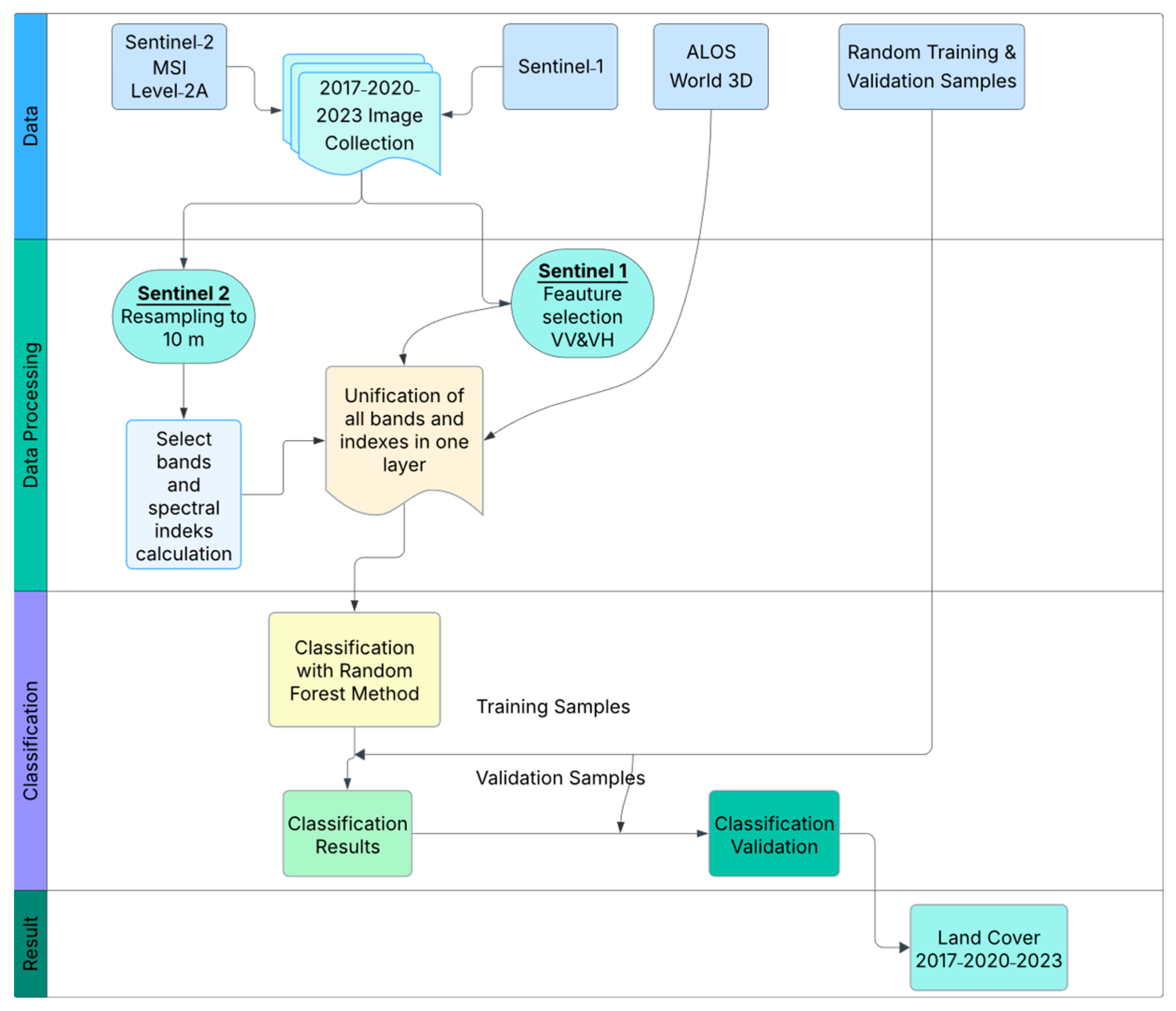
The methodology used to determine land cover for 2017, 2020, and 2023 is shown schematically in Figure 3. As illustrated in the figure, the raw data were first preprocessed, then classified. All these steps were carried out using Google Earth Engine (GEE), a cloud-based platform.
In the classification process, ten different spectral bands from satellite images, detailed in Table 1, were used. The Sentinel-2 MSI satellite provides various bands with spatial resolutions ranging from 10 m to 60 m. Among these bands, B2, B3, B4, and B8 have a resolution of 10 m, while B5, B6, B7, B8A, B11, and B12 are at 20 m. Additionally, bands B1 and B9 have a spatial resolution of 60 m.
Additionally, 14 surface spectral indices, with their formulas provided between Equation (1) and Equation (14), were used in the analyses [51,52,53,54,55,56,57,58,59,60,61,62,63]. These indices are calculated through various combinations of different spectral bands and enable a more detailed examination of the surface cover’s characteristic properties.
G r e e n   N o r m a l i z e d   D i f f e r e n c e   V e g e t a t i o n   I n d e x   G N D V I = B a n d   8 B a n d   3 B a n d   8 + B a n d   3
N o r m a l i z e d   D i f f e r e n c e   V e g e t a t i o n   I n d e x   ( N D V I ) = B a n d   8 B a n d   4 B a n d   8 + B a n d   4
N o r m a l i z e d   D i f f e r e n c e   W a t e r   I n d e x   ( N D W I ) = B a n d   3 B a n d   8 B a n d   3 + B a n d   8
M o d i f i c a t i o n   o f   n o r m a l i z e d   d i f f e r e n c e   w a t e r   i n d e x   ( M N D W I ) = B a n d   3 B a n d   11 B a n d   3 + B a n d   11
N o r m a l i z e d   D i f f e r e n c e   B u i l t U p I n d e x   ( N D B I ) = B a n d   11 B a n d   8 B a n d   11 + B a n d   8
B a r e   S o i l   I n d e x   ( B S I ) = B a n d   11 + B a n d   4 ( B a n d   8 + B a n d   2 ) B a n d   11 + B a n d   4 + ( B a n d   8 + B a n d   2 )
M o d i f i e d   B a r e   S o i l   I n d e x   ( M B S I ) = B a n d   11 B a n d   12 B a n d   8 B a n d   11 + B a n d   12 + B a n d   8 + 0.5
U r b a n   I n d e x   ( U I ) = B a n d   12 B a n d   8 B a n d   12 B a n d   8 + 1 × 100
E n h a n c e d   V e g e t a t i o n   I n d e x   ( E V I ) = 2.5 × B a n d   8 + B a n d   4 B a n t   8 + 6 × B a n t   4 7.5 × B a n d   2 + 1
S o i l   A d j u s t e d   V e g e t a t i o n   I n d e x   ( S A V I ) = 1.5 × B a n d   8 B a n d   4 B a n d   8 + B a n d   4 + 0.5
B u i l t u p   a r e a   E x t r a c t i o n   I n d e x   ( B A E I ) = B a n d   4 + 0.3 B a n d   3 + B a n d   11
A u t o m a t e d   W a t e r   E x t r a c t i o n   I n d e x   ( A W E I ) = B a n t   2 + 2.5 × B a n t   3 1.5 × B a n t   8 + B a n t   11 0.25 × B a n t   12
A u t o m a t e d   W a t e r   E x t r a c t i o n   I n d e x   S h a d o w   ( A W E I s h ) = 4 × B a n t   3 B a n t   11 0.25 × B a n t   8 + 2.75 × B a n t   12
M u l t i S p e c t r a l   W a t e r   I n d e x   ( M u W I R ) = 4 × B a n d   2 B a n d   3 B a n d   2 + B a n d   3 + 2 × B a n d   3 B a n d   8 B a n d   3 + B a n d   8 + 2 × B a n d   3 B a n d   12 B a n d   3 + B a n d   12 + B a n d   3 B a n d   11 B a n d   3 + B a n d   11 +
NDVI is a widely used index for detecting green vegetation. Healthy plants absorb radiation in the visible spectrum, especially in the blue (0.4–0.5 µm) and red (0.6–0.7 µm) bands, while reflecting in the green band (0.5–0.6 µm). This is why healthy plants appear green to the eye. Additionally, healthy plants exhibit high reflectance in the Near-Infrared (NIR) region between 0.7 and 1.3 µm. This is due to the internal structural properties of their leaves. NDVI is calculated by using the difference between high absorption in the red band and high reflectance in the NIR band [64]. The NDVI value ranges from −1 to +1, providing information about plant health [65].
GNDVI functions as a vegetation index, operating on principles like NDVI, but it sets itself apart by using the green spectral band instead of the red one. According to [57], GNDVI shows an increased sensitivity to variations in leaf chlorophyll content. This characteristic makes GNDVI an effective tool for monitoring plant health and density. As vegetation chlorophyll density increases, the GNDVI value also rises. Therefore, GNDVI is widely used in agriculture and forestry for stress detection, crop yield assessment, and monitoring plant growth.
NDWI was developed by [53] and is specifically used to detect and monitor surface water bodies. This index is derived by taking advantage of water’s strong reflectance in the green spectral band and its weak reflectance in the NIR region. Thus, it allows for a clear distinction between water bodies and other types of surface cover (e.g., vegetation or bare soil). However, in some cases where NDWI is limited, especially in urban areas where water surfaces blend with built-up surfaces, the MNDWI developed by [54] provides more effective results. MNDWI uses the difference between the green and shortwave infrared (SWIR) bands. This modification reduces the impact of built-up areas while making open water surfaces more prominent. Therefore, MNDWI is preferred for more accurate water detection, especially in regions with complex land cover [54].
NDBI is a widely used spectral index for identifying and mapping urban environment areas. It relies on the higher reflectance of artificial structures and bare soils in the SWIR bands compared to the NIR bands. In contrast, water surfaces show little reflection in the infrared spectrum, while healthy vegetation exhibits higher NIR reflectance than SWIR reflectance. The index ranges from −1 to +1; negative values indicate water bodies, while high positive values indicate densely built-up areas. Vegetation is generally characterized by low NDBI values [64].
The BSI value is calculated using blue, red, NIR, and SWIR bands. Near-infrared bands are used to evaluate the condition of bare soil and to identify alterations in soil properties [66].
BAEI is a spectral index developed by [61] to more effectively identify built-up areas in Landsat-8 imagery. This index highlights urban areas while minimizing the influence of mixed vegetation and soil.
UI is a remote sensing index used to identify and analyze urban areas. It is effectively used in detecting built-up areas, especially in densely urbanized regions [55].
EVI is an index developed to measure vegetation density and health. Compared to NDVI, it employs a more sophisticated formula and provides more effective corrections for atmospheric effects (such as aerosols and soil glare) [67].
SAVI is a vegetation index developed to minimize soil effects and provide a more accurate assessment of vegetation. It offers more dependable results than NDVI, especially in regions with sparse vegetation [60].
AWEI and AWEIsh are indices used to enhance the contrast between water surfaces and darker non-water surfaces, such as shadows and built-up areas [62]. The MuWIR is a spectral index used to simplify the analysis of water bodies [63].

2.4. Land Use and Land Cover Projection

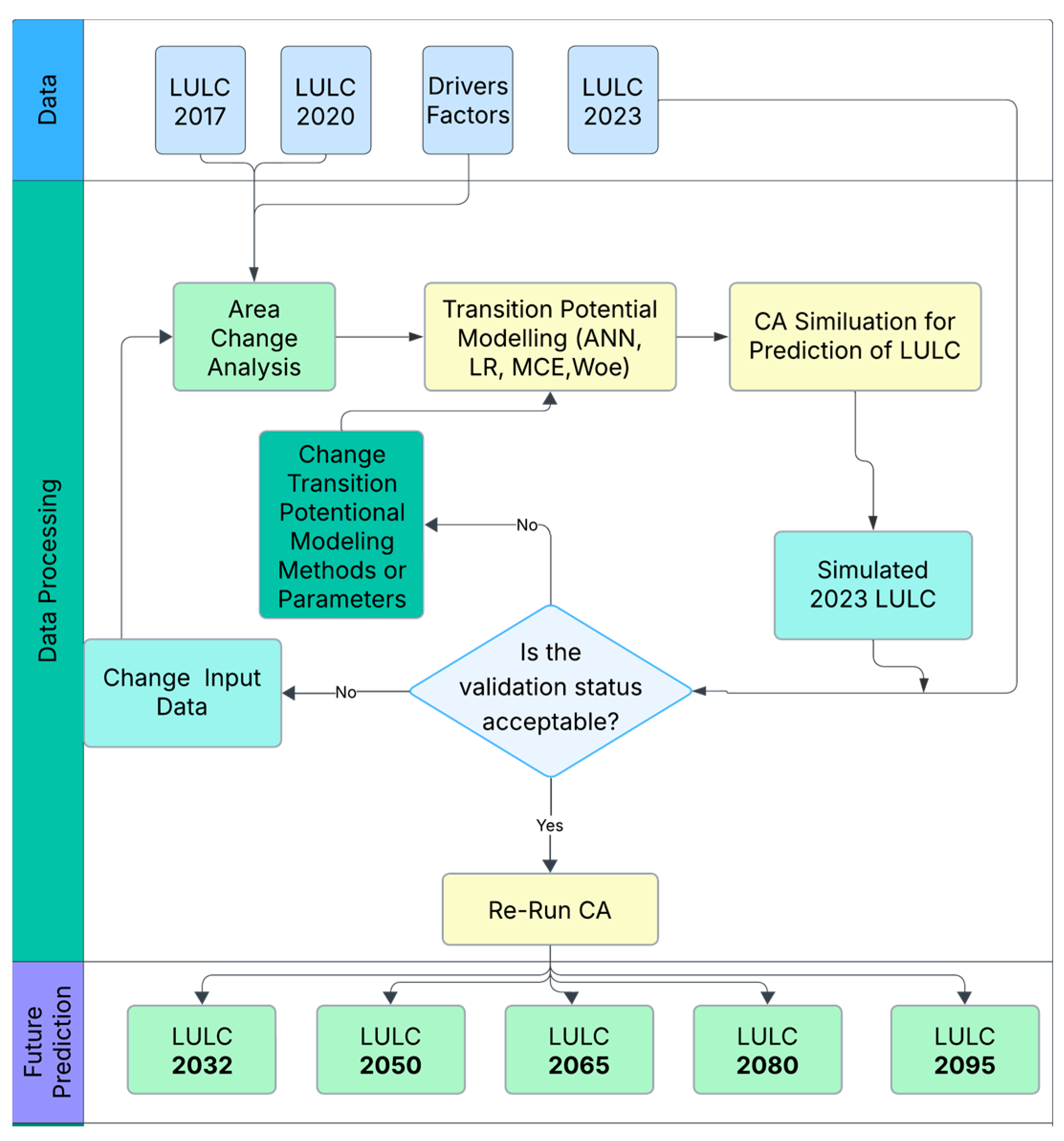
To model the spatial and temporal dynamics of land cover change and generate future land use projections, this study used the MOLUSCE (5.0.0) plugin in the QGIS (3.28.3-Firenze) environment. MOLUSCE provides a modular framework that includes various modeling algorithms, particularly Artificial Neural Networks (ANNs) and Markov chain approaches, for analyzing and simulating land use change patterns. The model utilizes historical land use maps and explanatory variables to determine transition probabilities and forecast future land use changes. Its predictions depend on the assumption that past land use trends will continue under similar conditions. The flow diagram in Figure 4 illustrates the process used for predicting and validating future land cover.
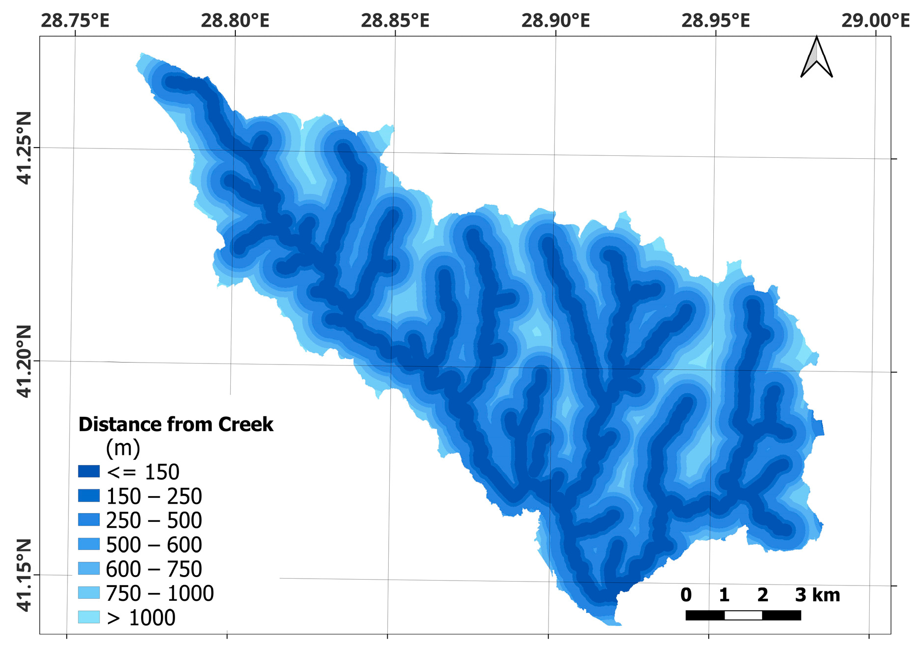
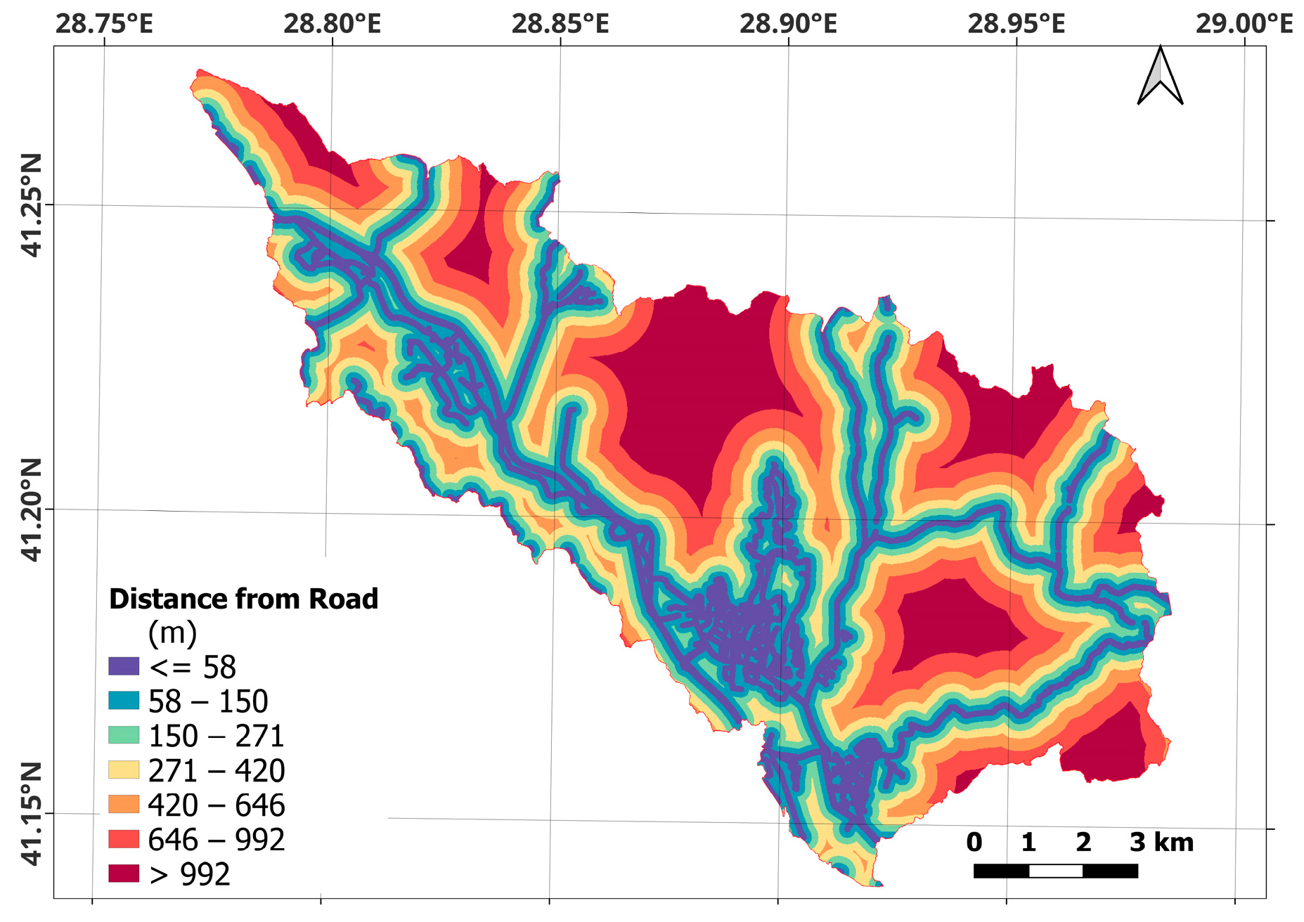
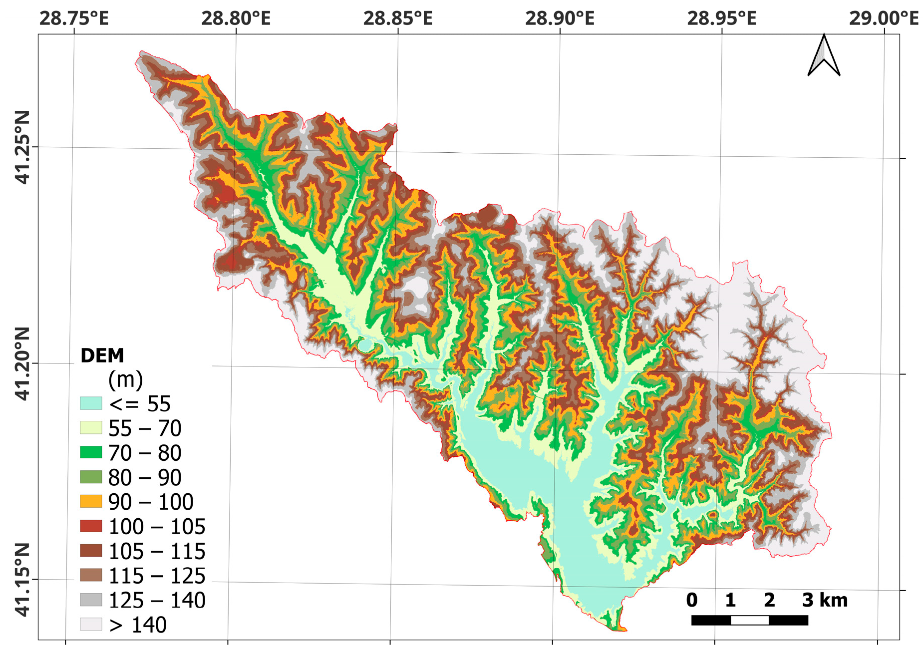
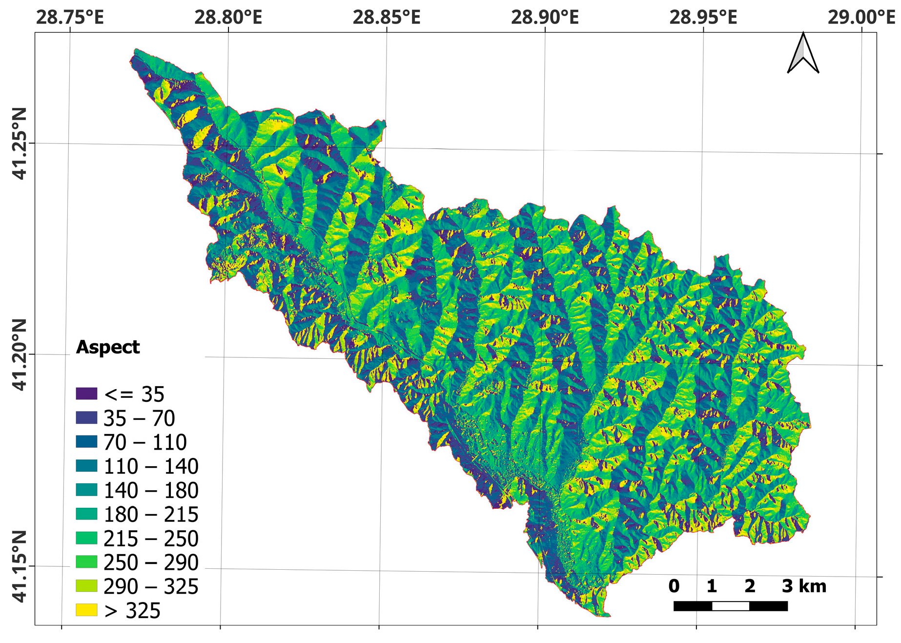
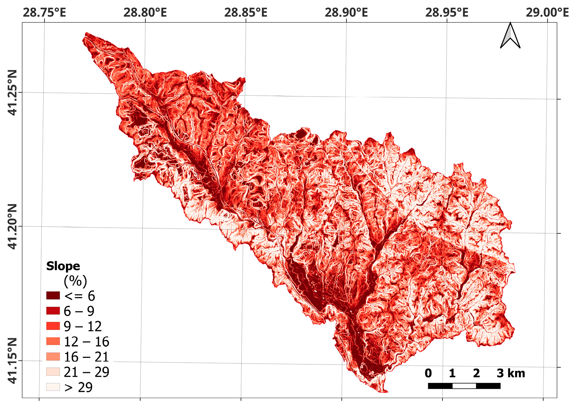
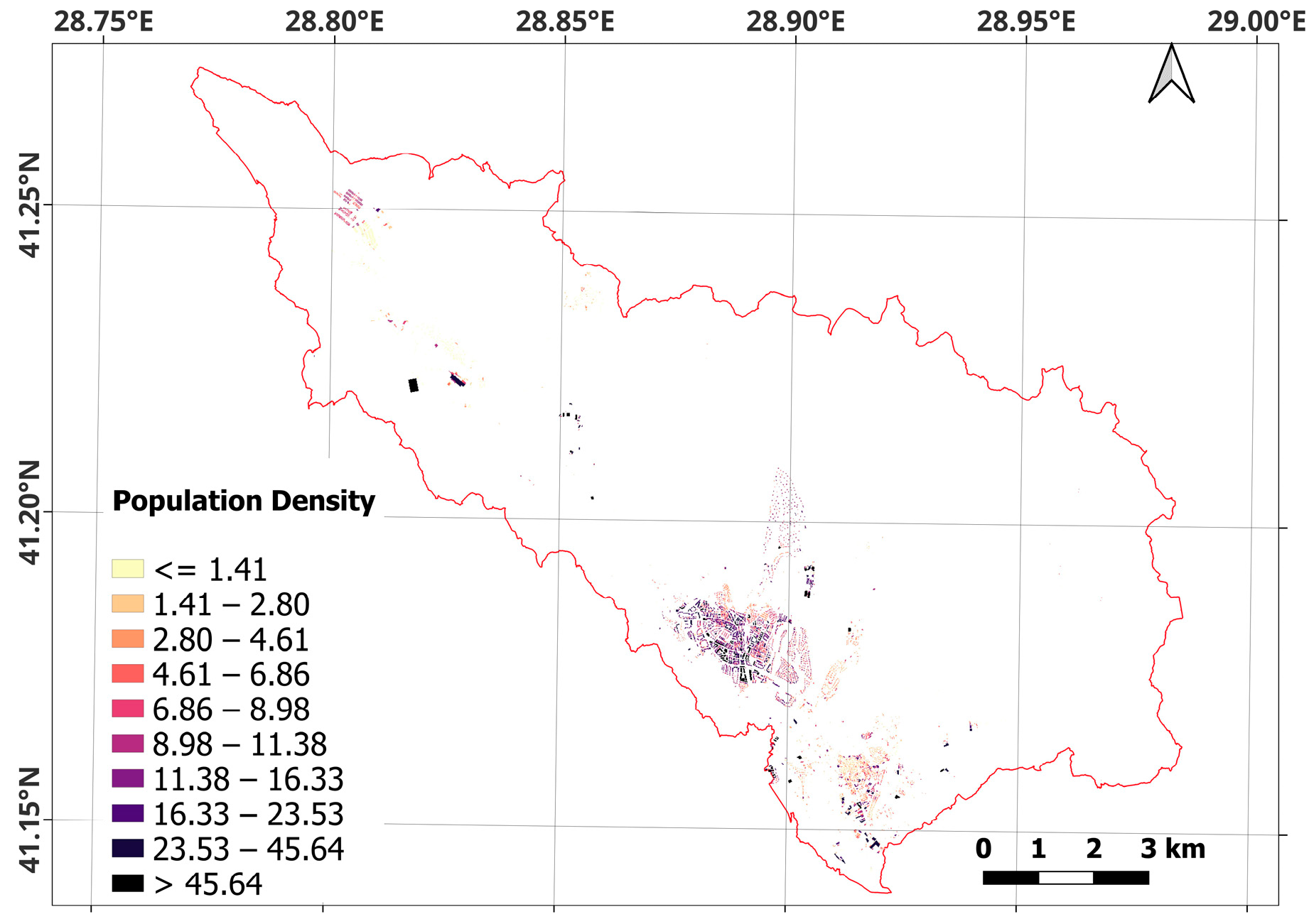
The modeling process began with a temporal comparison of land cover classification maps from earlier periods, enabling the creation of change matrices. Then, the factors driving land use changes were identified, and the corresponding spatial layers were generated. These factors include elevation, slope, and aspect maps derived from the Digital Elevation Model (DEM), along with Euclidean distances to roads, distance to hydrological networks (streams), and anthropogenic effects such as population density. All these factors were modeled in spatial data format using appropriate GIS software such as QGIS (3.28.3-Firenze) and ArcGIS (10.5). The resulting maps are shown in Figure 5, Figure 6, Figure 7, Figure 8, Figure 9 and Figure 10.
Within the MOLUSCE plugin, the Multilayer Perceptron Artificial Neural Network (MLP-ANN) successfully captured complex, non-linear relationships between past land cover changes and their driving factors. After training, the generated transition probabilities and spatial patterns were used to produce forward-looking land cover projections. The model’s accuracy was assessed by comparing simulated maps with actual observations, and various performance metrics, especially Kappa statistics, were calculated to evaluate the model’s reliability. The Multilayer Perceptron (MLP) approach was preferred for modeling land change dynamics.

2.5. Carbon Emission

The direct carbon emission coefficient approach quantifies emissions by combining each land use class’s land area with class-specific coefficients, allowing a systematic evaluation of their effects on the carbon cycle. In this framework, total carbon emissions attributable to land use are defined as the sum of (i) direct emissions occurring outside built-up areas and (ii) indirect emissions linked to human energy consumption within built-up areas. In non-built environments, such as arable cropland, forests, grasslands, pasture areas, wetlands, and unused or bare land, direct emissions mainly result from activities like using agricultural machinery, applying fertilizer, biotic respiration, and decomposition of soil organic matter.
The carbon emission coefficients used in this study were sourced from the literature [68,69,70,71,72,73], representing widely accepted average values. These coefficients reflect the mean carbon emission intensities for each land use/land cover (LULC) class. Using standardized coefficients was considered appropriate because the study’s goal is to assess relative changes over time rather than absolute figures. Localized coefficients could not be applied due to the lack of regional measurement data. However, country-specific coefficients, which account for Turkey’s natural gas consumption and electricity generation structure (as reported by TÜİK and the Ministry of Energy and Natural Resources) [74], were employed to estimate indirect carbon emissions related to energy use.
In this study, carbon emissions for non-built land classes are computed as the sum over classes of the product of each class’s area and its emission coefficient, as follows:
C A = A i α i
Here, CA denotes the total carbon emissions (tC) across land types, including arable land, forest, grassland–pasture, water/wetlands, and unused land. Ai is the area of land type i (hm2) and αi is the carbon emission coefficient for land type i(tC·hm−2). The coefficients adopted in this study are 0.422 tC·hm−2 for arable land, −0.644 tC·hm−2 for forests, -0.021 tC·hm−2 for grassland–pasture, −0.005 tC·hm−2 for unused land, and −0.253 tC·hm−2 for water/wetlands [68,69,70,71,72,73].
Indirect carbon emissions were included in the study by following the method in [74], which allocates Istanbul-wide total carbon emissions from natural gas and electricity use to residential areas, thereby calculating the carbon emission per unit area. According to [74], in 2018, natural gas consumption reached 7,659,839,016.62 m3, while electricity consumption was 40,452,118.85 MWh. The total carbon emissions amounted to 38,896,800.00 tons. Since the residential area in 2018 was 137,940.00 ha, the direct carbon emission per unit area was 281.98 tons CO2/ha. The analysis was based on the assumption that these unit emissions will stay constant through to 2095.

3. Results and Discussion

3.1. Discussion of Research Methods

Various land classification methods are available on the Google Earth Engine (GEE) platform, including Classification and Regression Trees (CARTs), Random Forest (RF), Naive Bayes, and Support Vector Machines (SVM). In previous studies [14,32,41,48], the Random Forest (RF) algorithm has often been favored for its high accuracy in land classification; therefore, the same method was employed in this study. The RF approach requires completing both training and validation steps to perform classification. Accordingly, for each year to be classified, six distinct classes (built-up areas, vegetation, forest, bare fields, water bodies, and roads) were defined, and training and validation samples were collected using high-resolution images marked on Google Earth Engine. For each year, a total of 540 samples were collected, with 90 samples assigned to each class. Of the collected data, 70% was allocated for training and 30% for validation. In this method, land classification was performed using a total of 28 predictors, including 150 decision trees and the following variables: B2, B3, B4, B5, B6, B7, B8, B8A, B11, B12, GNDVI, NDVI, NDWI, MNDWI, NDBI, BSI, MBSI, UI, EVI, SAVI, BAEI, VV, VH, AWAEI, AWAEIsh, MuWIR, elevation, and slope.
To assess the accuracy of classification algorithms, error matrices are used to measure how reliably the algorithms classify data. An error matrix is a numerical table organized in rows and columns, indicating to which class the samples from each original class have been assigned to.
The error matrix’s rows usually represent classification results (predicted values) from remote sensing data, while the columns typically show the reference data (ground truth). The error matrix allows for the computation of several accuracy metrics, including overall accuracy (OA), producer’s accuracy (PA), and user’s accuracy (UA), while also clearly displaying classification errors [75]. Overall accuracy (OA) is calculated by dividing the number of correctly classified samples (i.e., the values along the main diagonal of the matrix) by the total number of samples. However, only reporting this is not enough; displaying the entire matrix allows for the calculation of other accuracy metrics and provides insight into the confusion between map classes.
The producer’s and user’s accuracies in [75] are used not only to assess overall classification accuracy, but also to evaluate the accuracy within each class. A map producer may wish to know how accurately a particular class has been mapped (producer’s accuracy).
This value is determined by dividing the total number of reference samples for a class by the number of correctly classified samples for that class (the main diagonal value). User accuracy indicates how well the regions on the map labeled as belonging to a specific class actually do so. This figure is determined by dividing the total number of areas actually included in the classification by the total number of areas not included. Equations (16)–(18) present the mathematical formulas for these accuracies [76].
12mTotal of Row
ni+
1n11n12n1mn1+
2n21n22n2mn2+
mnm1nm2nmmnk+
Total of Column: n+jn+1n+1n+1n
i: Rows—Classification
j: Columns—References
O A = i = 1 m n i i n
P A i = n i i n i +
U A j = n j j n j +

3.2. Comparison with Existing Studies

In the literature, some studies [14,36] have conducted analyses using only satellite imagery, while others have also incorporated spectral indices [48]. For instance, in [48], the author utilized six different spectral indices in his study, whereas in the present research, the prediction of land cover classes was carried out using fourteen spectral indices. The 14 spectral indices used in this study were chosen because they better discriminate between different surface types (vegetation, water bodies, built-up areas, and bare soil) and capture the heterogeneous urban structure of the study area. Vegetation indices such as NDVI, EVI, and SAVI reflect the density of green areas, while indices like NDBI, UI, and NDBAI are effective for identifying urban regions. To distinguish water surfaces, NDWI and MNDWI were used, and to detect bare soil, indices like BSI were applied. The combined use of these indices aims to improve the accuracy of land cover classification. Additionally, elevation and slope factors were incorporated into the land cover classification process. All indices are listed in Section 2.3.
Unlike the study by in [48], various simulations aimed at predicting the LULC change map for 2023 were conducted, using land cover data produced with more spectral indices, along with slope and elevation variables.

3.3. Limitations

The model’s long-term projections, extending to 2095, assume that current trends will continue under similar conditions. However, long-term validation is not feasible due to the absence of actual observational data for future periods. This limitation is considered one of the main constraints of the study. Therefore, the future projections should be seen as trend indicators rather than exact predictions. It is recommended that future studies include scenario-based simulations, ensemble modeling, and multiple machine learning algorithms to decrease these uncertainties. Using global average emission coefficients due to the lack of regional measurements can create some uncertainty in regional predictions. Therefore, the long-term results should be interpreted as indicators of trends rather than exact predictions. Although the indirect carbon emission coefficient used in this study was regarded as a constant, long-term advances in energy technologies, sustainability policies, and carbon reduction strategies could significantly affect this value. To reduce uncertainties and enhance prediction accuracy, future research should focus on obtaining local measurements of carbon intensity, using time-series-based dynamic or scenario-specific emission coefficients, and applying scenario-based simulations, ensemble modeling, and multiple machine learning algorithms.

3.4. Future Projection

The intra-annual changes in NDVI reveal that, in May 2020, there was a noticeable increase in NDVI values, a pattern not seen in the other years. After July, a decline in NDVI values became evident. In 2017, an upward trend was observed from late September to mid-October. In contrast, no clear trend was detected throughout the months of 2023.
The accuracy values of the classification results for 2017, 2020, and 2023 are shown in Table 2. In all years analyzed, both parameters achieved accuracy rates above 92%. The overall accuracy values were calculated as 0.9847, 0.9847, and 0.9797, respectively. These results, like those reported in other studies [14,48], demonstrate a high level of accuracy, exceeding 90%.
Kappa analysis is a discrete multivariate technique used to assess accuracy by statistically testing whether two error matrices differ significantly from each other [77].
It is a reliable method for testing significant differences between various error matrices, and Kappa analysis is effectively used for this purpose. For instance, maps of the same area can be generated using both algorithms, and their error matrices compared, to demonstrate how much better a new classification algorithm is compared to a commonly used one. The statistical superiority of the new algorithm can then be evaluated with the Kappa analysis [76]. A Kappa value close to 1 indicates a decrease in error rate and an improvement in classification accuracy. The study’s Kappa values for 2017, 2020, and 2023 were 0.9815, 0.9816, and 0.9757, respectively.
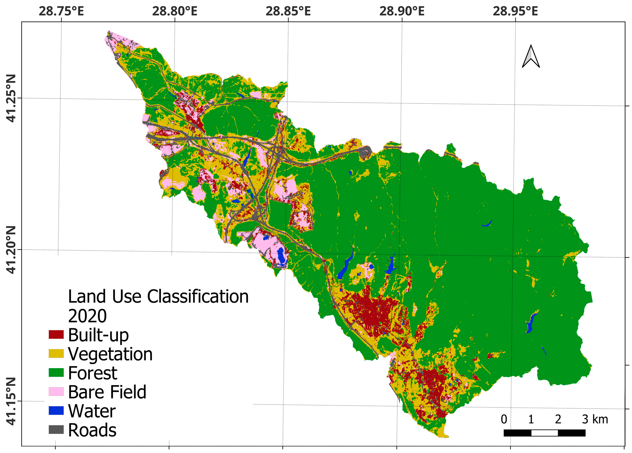
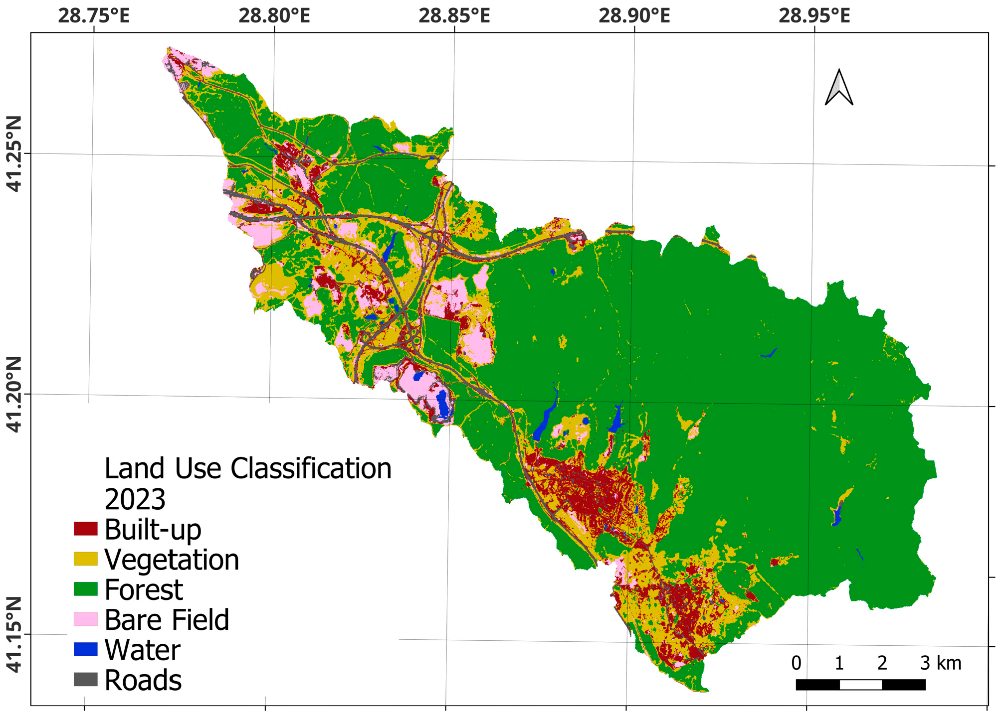
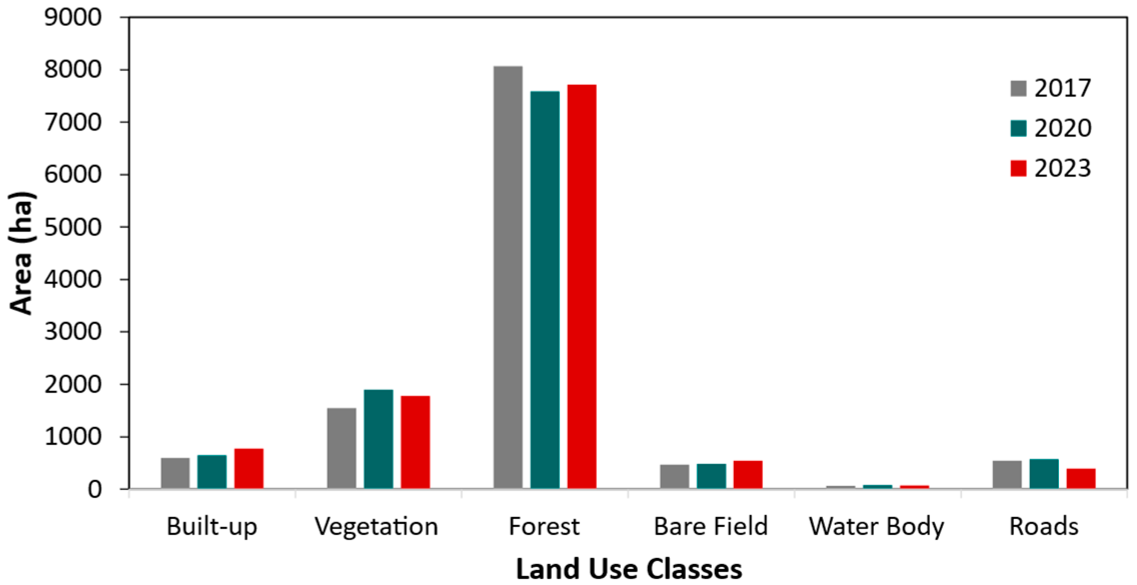
As a result of the study, maps for each class for 2017, 2020, and 2023 are shown in Figure 11, Figure 12, and Figure 13, respectively. Additionally, the spatial distributions within the study area for each year are depicted in Figure 14.
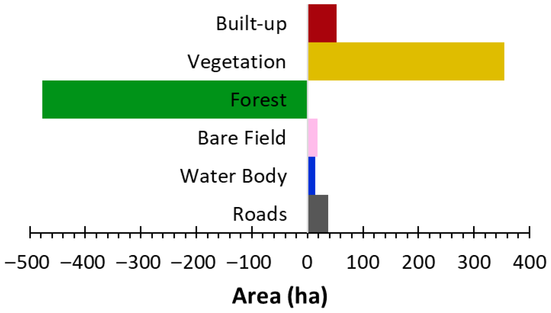
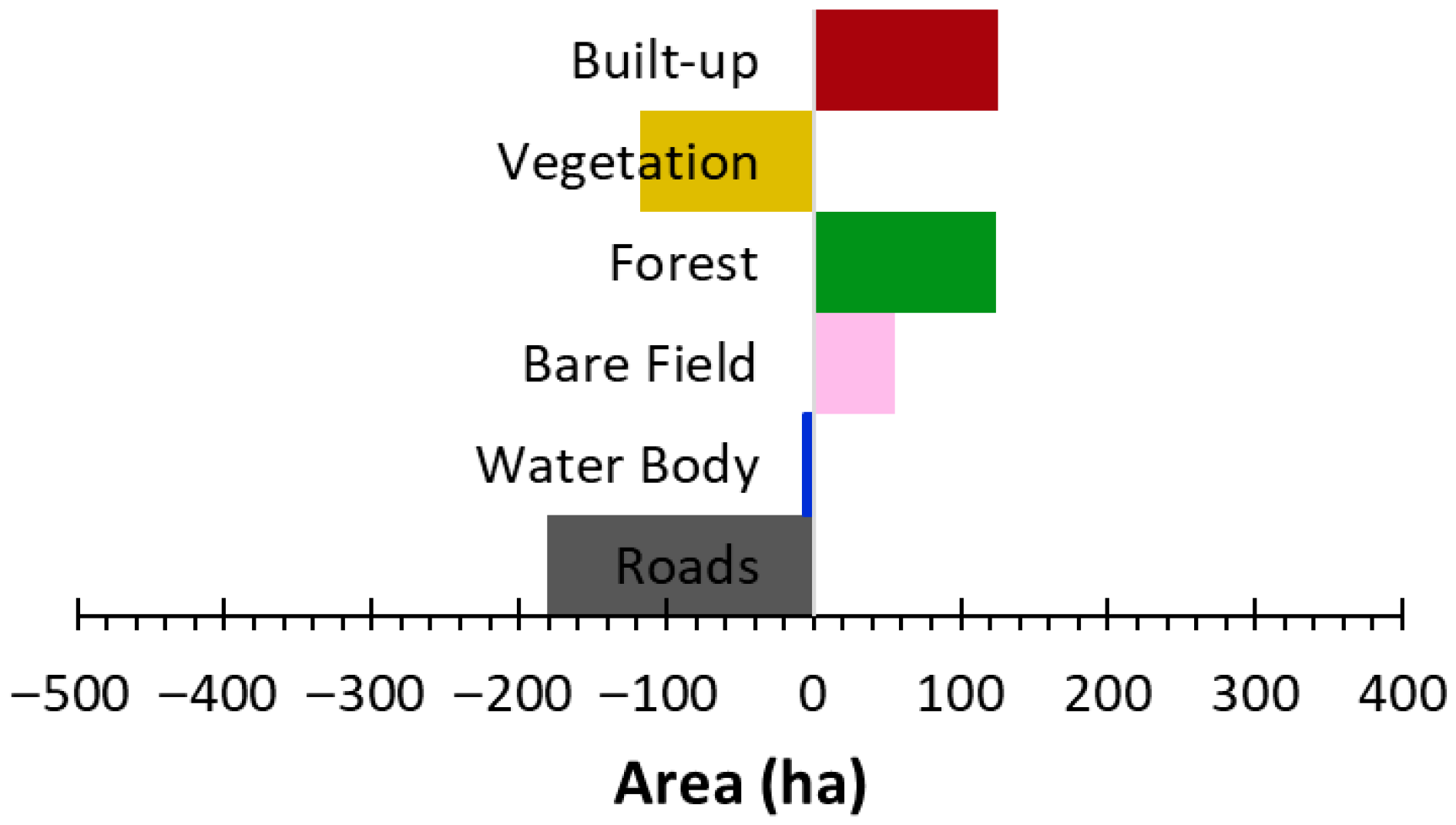
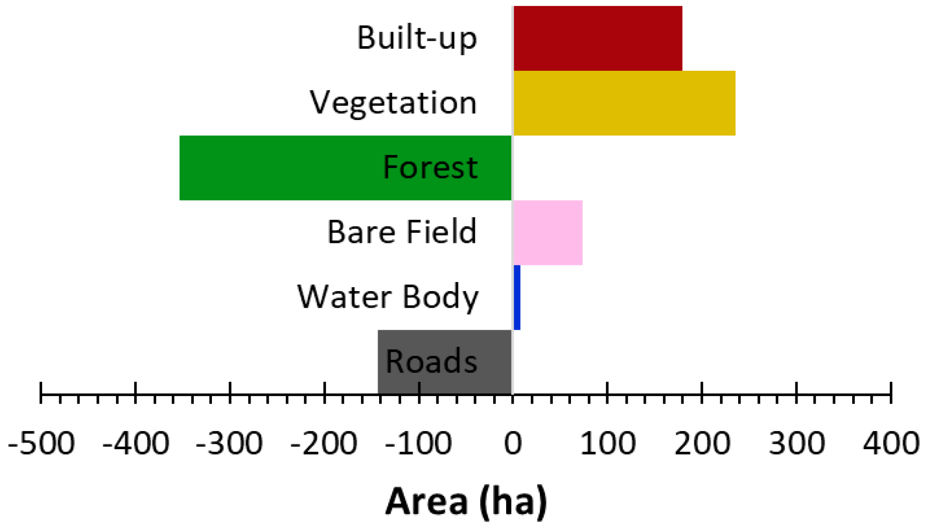
An analysis of this graph shows a rising trend in built-up and bare fields from 2017 to 2023. The land cover type transitions for 2017 and 2020 are detailed in Table 3, while the extent of these changes is depicted in Figure 15. During this period, it was observed that 5.6% of forest areas converted to vegetation, and 10.3% of vegetation areas shifted to built-up areas. Examining the changes between 2020 and 2023 in Table 4, it is evident that 13.6% of bare fields were converted to built-up areas, and 15.9% were transformed into vegetation. Although forest areas increased during these years, vegetation areas decreased. The extent of these changes is shown in Figure 16. The changes in vegetation types from 2017 to 2023 are outlined in Table 5. According to this table, forest and road areas decreased, while all other classes saw increases. Most changes in forest areas resulted from conversion to vegetation, whereas road areas were primarily transformed into built-up and bare fields. Consequently, the proportion of built-up and bare fields within the total area has steadily grown each year. The extent of these changes is illustrated in Figure 17.
These simulations were conducted using various combinations of spatial variable factors, and the scenarios incorporating these combinations are shown in Table 6. For land cover class projection, the Artificial Neural Network (ANN) method was used, with the following parameters: neighborhood size of 1, 1000 iterations, 10 hidden layers, and a learning rate and momentum set to 0.001 [35,43,78]. Table 7 presents a comparison of the overall accuracy and maximum Kappa coefficients for the different spatial variable combinations. Based on the results, the S1 scenario, which includes all variable factors, achieved the highest performance, with a Kappa value of 0.84 and an accuracy rate of 91.88% (Table 7). This suggests that the model has an acceptable level of accuracy [78,79].
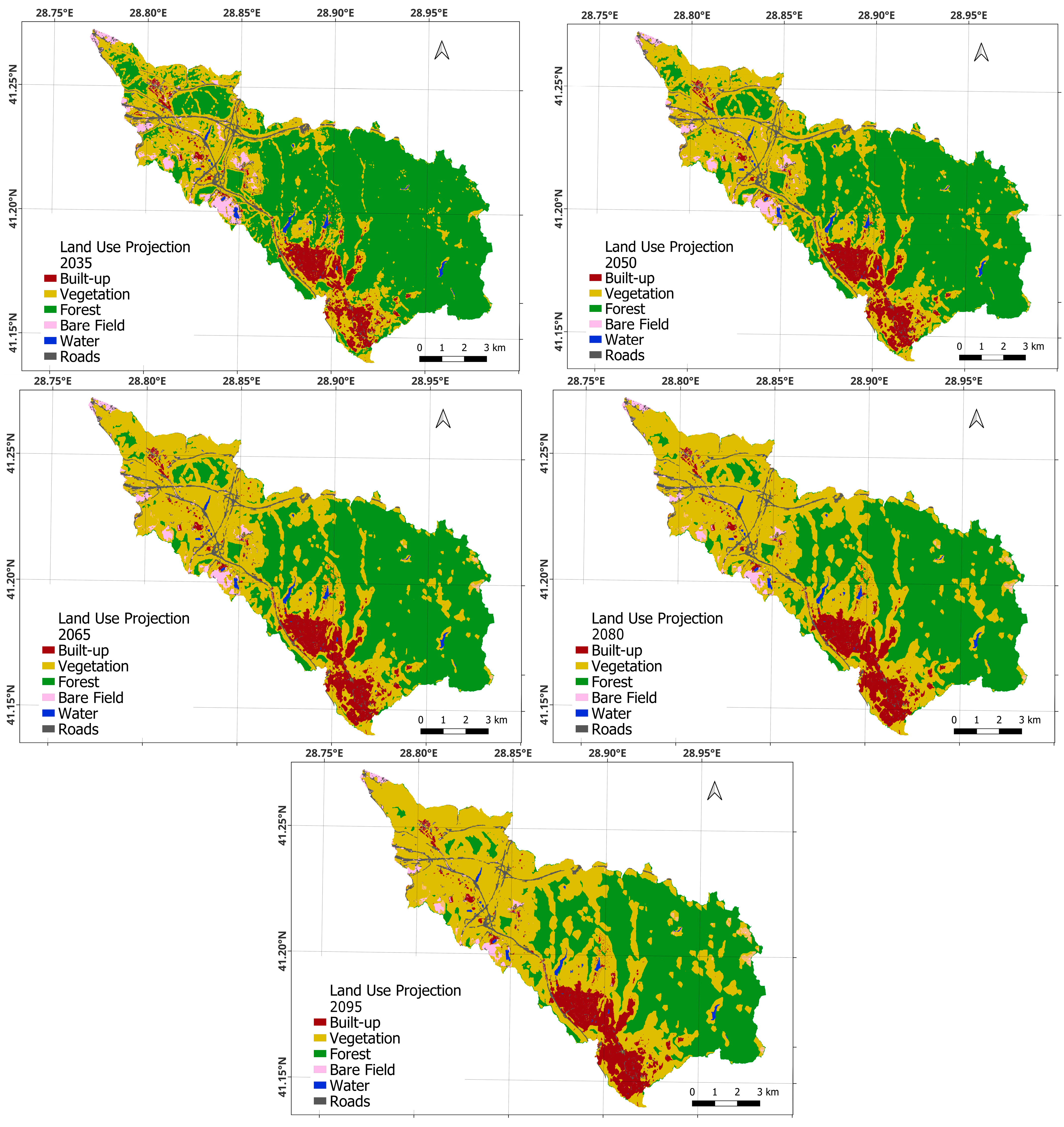
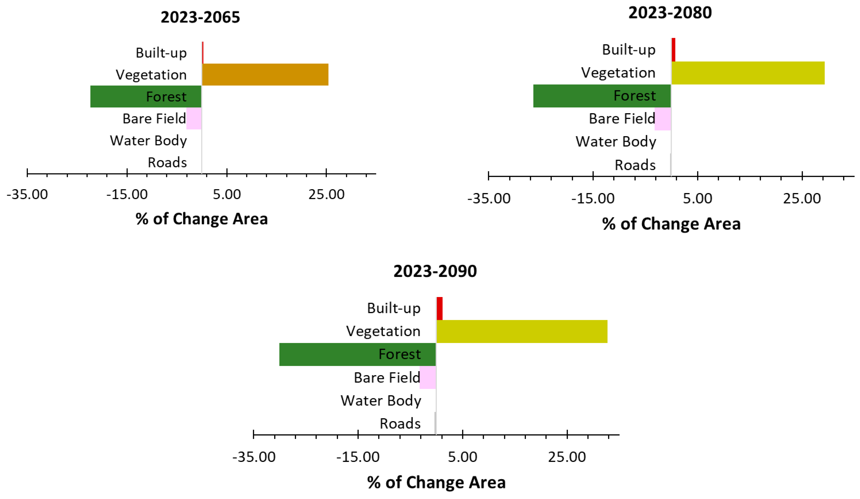
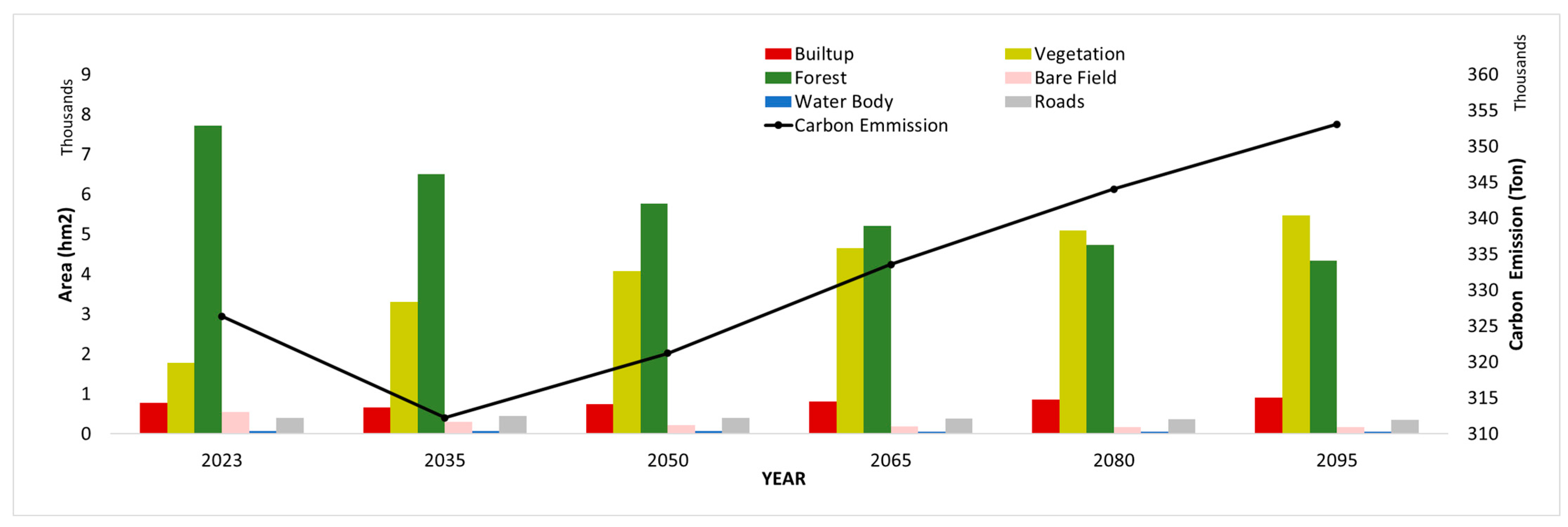
After completing the validation phase, land use projections for 2035, 2050, 2065, 2080, and 2095 were generated using the cellular automata (CA) model. The projected land use maps for these years are shown in Figure 18. Figure 18 and Figure 19 reveal a decreasing trend in the forest and bare land areas, while vegetated and built-up regions expand. It also appears that vegetated areas may gradually transform into built-up zones over time. Meanwhile, changes in water bodies are minimal.
Forests, water bodies, and bare areas, which have emission-reducing effects, help lower carbon emissions as they increase. In contrast, increases in vegetated (primarily agricultural) areas, roads, and built-up areas raise carbon emissions. After 2035, if no measures are taken, the upward trend in carbon emissions is expected to intensify. In 2035, compared to 2023, although urbanization decreases by approximately 0.93%, vegetated areas increase by about 13%, and forest areas decrease by about 10.7%. Total carbon emissions are observed to be lower than in 2023 (Figure 20).

4. Conclusions

For the study area within the boundaries of the Kağıthane Basin in Istanbul, land use classifications for 2017, 2020, and 2023 were generated on the Google Earth Engine (GEE) platform using the Random Forest algorithm. High-resolution sample data were collected for six different land cover classes (built-up, vegetation, forest, bare field, water bodies, and roads), which were then used for model training and validation. The outcomes demonstrate the reliability and efficiency of the developed classification model, with high producer’s and user’s accuracies and an overall accuracy rate of roughly 98%. Furthermore, Kappa coefficients exceeding 0.97 indicate that the classification is statistically significant and consistent.
An analysis of land cover changes over time shows that forest areas have declined while built-up and bare fields have increased. These alterations reflect the effects of urbanization and intensifying anthropogenic land use in the region. Throughout the study period, vegetation areas showed periodic fluctuations. This land cover class has remained relatively stable, as evidenced by the lack of notable spatial changes observed in water bodies. These results are further supported by the study area’s population growth of 16.59% over the previous ten years.
In the land use projection analysis covering 2023 to 2095, a short-term decrease in built-up areas is anticipated; however, vegetation areas are expected to be gradually converted into built-up areas over the following years, leading to a renewed increase in built-up areas in the long term. During this process, both forest and bare fields are projected to decrease. An examination of simulations across years reveals a consistent decrease in forest areas and an upward trend in vegetated and built-up areas. This projection provides essential inputs for regional planning and natural resource management.
The simulations indicate a continuous decline in forest areas and an increasing trend in arable and built-up areas, suggesting a negative picture for carbon emissions. The reduction in forests decreases the atmosphere’s capacity to absorb carbon dioxide, thereby increasing net carbon emissions. The expansion of arable land can reduce organic carbon and increase greenhouse gas emissions, depending on the type of agricultural practice. In contrast, the growth of built-up areas increases emissions from construction and energy use, expanding the overall carbon footprint. This pattern has the potential to raise the region’s overall carbon emissions and complicate efforts to combat climate change.
In conclusion, the land classification and projection study, carried out using the Random Forest algorithm on the GEE platform, has shown that it is an effective method for monitoring land use dynamics in the region and for supporting future planning with high accuracy and reliability. The decrease in forest areas due to population growth and the conversion of these areas into bare fields for construction increase the risk of future flooding, environmental pollution, and carbon emissions. For this reason, it is recommended that appropriate solutions be developed and settlement plans prepared in the study area to prevent the negative impact of these issues. The findings provide guidance for developing sustainable land use policies that account for the impacts of urban growth on carbon emissions. In particular, it is recommended that such spatial analyses be utilized as fundamental decision-support tools in green infrastructure planning, land management, and the formulation of climate-friendly urban strategies.

Author Contributions

B.K.: writing—original draft, methodology, conceptualization; H.A.: review and editing, supervision. All authors have read and agreed to the published version of the manuscript.

Funding

This research received no external funding.

Institutional Review Board Statement

Not applicable.

Informed Consent Statement

Not applicable.

Data Availability Statement

Some of the data used in this study are available in public repositories, while additional data are available from the corresponding author upon reasonable request.

Acknowledgments

The author gratefully acknowledges the support received under the Scientific and Technological Research Council of Türkiye (TÜBİTAK)—Scientist Support Programs Directorate (BİDEB), 2211—National PhD Scholarship Program. The author also thanks Istanbul Water and Sewerage Administration (İSKİ) for providing some of the data used in this study.

Conflicts of Interest

The authors declare no conflicts of interest.

References

  1. Leeson, G.W. The Growth, Ageing and Urbanisation of Our World. J. Popul. Ageing 2018, 11, 107–115. [Google Scholar] [CrossRef]
  2. Huang, K.; Li, X.; Liu, X.; Seto, K.C. Projecting Global Urban Land Expansion and Heat Island Intensification through 2050. Environ. Res. Lett. 2019, 14, 114037. [Google Scholar] [CrossRef]
  3. Turkish Statistical Institute. TSI. Available online: https://biruni.tuik.gov.tr/medas/?kn=95&locale=tr (accessed on 26 June 2025).
  4. IPCC. Climate Change 2014: Impacts, Adaptation and Vulnerability; Cambridge University Press: Cambridge, UK, 2014. [Google Scholar]
  5. Hinge, G.; Surampalli, R.Y.; Goyal, M.K. Regional Carbon Fluxes from Land-Use Conversion and Land-Use Management in Northeast India. J. Hazard. Toxic Radioact. Waste 2018, 22, 04018016. [Google Scholar] [CrossRef]
  6. Zhang, P.; He, J.; Hong, X.; Zhang, W.; Qin, C.; Pang, B.; Li, Y.; Liu, Y. Carbon Sources/Sinks Analysis of Land Use Changes in China Based on Data Envelopment Analysis. J. Clean. Prod. 2018, 204, 702–711. [Google Scholar] [CrossRef]
  7. Huang, Y.; Shen, L.; Liu, H. Grey Relational Analysis, Principal Component Analysis and Forecasting of Carbon Emissions Based on Long Short-Term Memory in China. J. Clean. Prod. 2019, 209, 415–423. [Google Scholar] [CrossRef]
  8. Liu, H.; Xing, L.; Wang, C.; Zhang, H. Sustainability Assessment of Coupled Human and Natural Systems from the Perspective of the Supply and Demand of Ecosystem Services. Front. Earth Sci. 2022, 10, 1025787. [Google Scholar] [CrossRef]
  9. Ashaolu, E.D.; Olorunfemi, J.F.; Ifabiyi, I.P. Assessing the Spatio-Temporal Pattern of Land Use and Land Cover Changes in Osun Drainage Basin, Nigeria. J. Environ. Geogr. 2019, 12, 41–50. [Google Scholar] [CrossRef]
  10. Msovu, U.E.; Mulungu, D.M.M.; Nobert, J.K.; Mahoo, H. Land Use/Cover Change and Their Impacts on Streamflow in Kikuletwa Catchment of Pangani River Basin, Tanzania. Tanzan. J. Eng. Technol. 2019, 38, 171–192. [Google Scholar] [CrossRef]
  11. Ullah, M.S.; Shapla, T.; Hossain, M.A.; Hasan, M.H. Delineating Agricultural Landuse Change Using Geospatial Techniques and Markov Model in the Tarakanda Upazila of Mymensingh, Bangladesh and Future Prediction. Dhaka Univ. J. Earth Environ. Sci. 2020, 8, 19–31. [Google Scholar] [CrossRef]
  12. Amgoth, A.; Rani, H.P.; Jayakumar, K.V. Exploring LULC Changes in Pakhal Lake Area, Telangana, India Using QGIS MOLUSCE Plugin. Spat. Inf. Res. 2023, 31, 429–438. [Google Scholar] [CrossRef]
  13. Gao, C.; Cheng, D.; Iqbal, J.; Yao, S. Spatiotemporal Change Analysis and Prediction of the Great Yellow River Region (GYRR) Land Cover and the Relationship Analysis with Mountain Hazards. Land 2023, 12, 340. [Google Scholar] [CrossRef]
  14. Lukas, P.; Melesse, A.M.; Kenea, T.T. Prediction of Future Land Use/Land Cover Changes Using a Coupled CA-ANN Model in the Upper Omo–Gibe River Basin, Ethiopia. Remote Sens. 2023, 15, 1148. [Google Scholar] [CrossRef]
  15. Iacono, M.; Levinson, D.; El-Geneidy, A.; Wasfi, R. A Markov Chain Model of Land Use Change. TeMA J. Land Use Mobil. Environ. TeMA 2015, 8, 263–276. [Google Scholar] [CrossRef]
  16. Dey, N.N.; Al Rakib, A.; Kafy, A.A.; Raikwar, V. Geospatial Modelling of Changes in Land Use/Land Cover Dynamics Using Multi-Layer Perception Markov Chain Model in Rajshahi City, Bangladesh. Environ. Chall. 2021, 4, 100148. [Google Scholar] [CrossRef]
  17. de Almeida, C.M.; Batty, M.; Monteiro, A.M.V.; Câmara, G.; Soares-Filho, B.S.; Cerqueira, G.C.; Pennachin, C.L. Stochastic Cellular Automata Modeling of Urban Land Use Dynamics: Empirical Development and Estimation. Comput. Environ. Urban Syst. 2003, 27, 481–509. [Google Scholar] [CrossRef]
  18. Liu, X.; Liang, X.; Li, X.; Xu, X.; Ou, J.; Chen, Y.; Li, S.; Wang, S.; Pei, F. A Future Land Use Simulation Model (FLUS) for Simulating Multiple Land Use Scenarios by Coupling Human and Natural Effects. Landsc. Urban Plan. 2017, 168, 94–116. [Google Scholar] [CrossRef]
  19. Wang, J.; Zhang, J.; Xiong, N.; Liang, B.; Wang, Z.; Cressey, E.L. Spatial and Temporal Variation, Simulation and Prediction of Land Use in Ecological Conservation Area of Western Beijing. Remote Sens. 2022, 14, 1452. [Google Scholar] [CrossRef]
  20. Sang, L.; Zhang, C.; Yang, J.; Zhu, D.; Yun, W. Simulation of Land Use Spatial Pattern of Towns and Villages Based on CA-Markov Model. Math. Comput. Model. 2011, 54, 938–943. [Google Scholar] [CrossRef]
  21. Hamad, R.; Balzter, H.; Kolo, K. Predicting Land Use/Land Cover Changes Using a CA-Markov Model under Two Different Scenarios. Sustainability 2018, 10, 3421. [Google Scholar] [CrossRef]
  22. Jantz, C.A.; Goetz, S.J.; Shelley, M.K. Using the SLEUTH Urban Growth Model to Simulate the Impacts of Future Policy Scenarios on Urban Land Use in the Baltimore-Washington Metropolitan Area. Environ. Plan. B Plan. Des. 2004, 31, 938–943. [Google Scholar] [CrossRef]
  23. Mahiny, A.S.; Clarke, K.C. Guiding SLEUTH Land-Use/Land-Cover Change Modeling Using Multicriteria Evaluation: Towards Dynamic Sustainable Land-Use Planning. Environ. Plan. B Plan. Des. 2012, 39, 925–944. [Google Scholar] [CrossRef]
  24. De Fioravante, P.; Luti, T.; Cavalli, A.; Giuliani, C.; Dichicco, P.; Marchetti, M.; Chirici, G.; Congedo, L.; Munafò, M. Multispectral Sentinel-2 and Sar Sentinel-1 Integration for Automatic Land Cover Classification. Land 2021, 10, 611. [Google Scholar] [CrossRef]
  25. Chakhar, A.; Hernández-López, D.; Ballesteros, R.; Moreno, M.A. Improving the Accuracy of Multiple Algorithms for Crop Classification by Integrating Sentinel-1 Observations with Sentinel-2 Data. Remote Sens. 2021, 13, 243. [Google Scholar] [CrossRef]
  26. Faqe Ibrahim, G.R.; Rasul, A.; Abdullah, H. Improving Crop Classification Accuracy with Integrated Sentinel-1 and Sentinel-2 Data: A Case Study of Barley and Wheat. J. Geovisualization Spat. Anal. 2023, 7, 22. [Google Scholar] [CrossRef]
  27. Koukiou, G. SAR Features and Techniques for Urban Planning—A Review. Remote Sens. 2024, 16, 1923. [Google Scholar] [CrossRef]
  28. Guan, T.; Chang, S.; Deng, Y.; Xue, F.; Wang, C.; Jia, X. Oriented SAR Ship Detection Based on Edge Deformable Convolution and Point Set Representation. Remote Sens. 2025, 17, 1612. [Google Scholar] [CrossRef]
  29. Li, M.; Hong, L.; Guo, J.; Zhu, A. Automated Extraction of Lake Water Bodies in Complex Geographical Environments by Fusing Sentinel-1/2 Data. Water 2022, 14, 30. [Google Scholar] [CrossRef]
  30. Nasiri, V.; Deljouei, A.; Moradi, F.; Sadeghi, S.M.M.; Borz, S.A. Land Use and Land Cover Mapping Using Sentinel-2, Landsat-8 Satellite Images, and Google Earth Engine: A Comparison of Two Composition Methods. Remote Sens. 2022, 14, 1977. [Google Scholar] [CrossRef]
  31. Islam, I.; Tonny, K.F.; Hoque, M.Z.; Abdullah, H.M.; Khan, B.M.; Islam, K.H.S.; Prodhan, F.A.; Ahmed, M.; Mohana, N.T.; Ferdush, J. Monitoring and Prediction of Land Use Land Cover Change of Chittagong Metropolitan City by CA-ANN Model. Int. J. Environ. Sci. Technol. 2024, 21, 6275–6286. [Google Scholar] [CrossRef]
  32. Halmy, M.W.A.; Gessler, P.E.; Hicke, J.A.; Salem, B.B. Land Use/Land Cover Change Detection and Prediction in the North-Western Coastal Desert of Egypt Using Markov-CA. Appl. Geogr. 2015, 63, 101–112. [Google Scholar] [CrossRef]
  33. Hyandye, C.; Martz, L.W. A Markovian and Cellular Automata Land-Use Change Predictive Model of the Usangu Catchment. Int. J. Remote Sens. 2017, 38, 64–81. [Google Scholar] [CrossRef]
  34. Alqadhi, S.; Mallick, J.; Balha, A.; Bindajam, A.; Singh, C.K.; Hoa, P.V. Spatial and Decadal Prediction of Land Use/Land Cover Using Multi-Layer Perceptron-Neural Network (MLP-NN) Algorithm for a Semi-Arid Region of Asir, Saudi Arabia. Earth Sci. Inform. 2021, 14, 1547–1562. [Google Scholar] [CrossRef]
  35. Kamaraj, M.; Rangarajan, S. Predicting the Future Land Use and Land Cover Changes for Bhavani Basin, Tamil Nadu, India, Using QGIS MOLUSCE Plugin. Environ. Sci. Pollut. Res. 2022, 29, 86337–86348. [Google Scholar] [CrossRef]
  36. Muhammad, R.; Zhang, W.; Abbas, Z.; Guo, F.; Gwiazdzinski, L. Spatiotemporal Change Analysis and Prediction of Future Land Use and Land Cover Changes Using QGIS MOLUSCE Plugin and Remote Sensing Big Data: A Case Study of Linyi, China. Land 2022, 11, 419. [Google Scholar] [CrossRef]
  37. Getachew, B.; Manjunatha, B.R.; Bhat, H.G. Modeling Projected Impacts of Climate and Land Use/Land Cover Changes on Hydrological Responses in the Lake Tana Basin, Upper Blue Nile River Basin, Ethiopia. J. Hydrol. 2021, 595, 125974. [Google Scholar] [CrossRef]
  38. Yirsaw, E.; Wu, W.; Shi, X.; Temesgen, H.; Bekele, B. Land Use/Land Cover Change Modeling and the Prediction of Subsequent Changes in Ecosystem Service Values in a Coastal Area of China, the Su-Xi-Chang Region. Sustainability 2017, 9, 1204. [Google Scholar] [CrossRef]
  39. Admas, M.; Melesse, A.M.; Tegegne, G. Predicting the Impacts of Land Use/Cover and Climate Changes on Water and Sediment Flows in the Megech Watershed, Upper Blue Nile Basin. Remote Sens. 2024, 16, 2385. [Google Scholar] [CrossRef]
  40. Wang, S.W.; Munkhnasan, L.; Lee, W.K. Land Use and Land Cover Change Detection and Prediction in Bhutan’s High Altitude City of Thimphu, Using Cellular Automata and Markov Chain. Environ. Chall. 2021, 2, 100017. [Google Scholar] [CrossRef]
  41. Hakim, A.M.Y.; Baja, S.; Rampisela, D.A.; Arif, S. Modelling Land Use/Land Cover Changes Prediction Using Multi-Layer Perceptron Neural Network (MLPNN): A Case Study in Makassar City, Indonesia. Int. J. Environ. Stud. 2021, 78, 301–318. [Google Scholar] [CrossRef]
  42. Liping, C.; Yujun, S.; Saeed, S. Monitoring and Predicting Land Use and Land Cover Changes Using Remote Sensing and GIS Techniques—A Case Study of a Hilly Area, Jiangle, China. PLoS ONE 2018, 13, e0200493. [Google Scholar] [CrossRef]
  43. El-Tantawi, A.M.; Bao, A.; Chang, C.; Liu, Y. Monitoring and Predicting Land Use/Cover Changes in the Aksu-Tarim River Basin, Xinjiang-China (1990–2030). Environ. Monit. Assess. 2019, 191, 480. [Google Scholar] [CrossRef]
  44. Baghel, S.; Kothari, M.K.; Tripathi, M.P.; Singh, P.K.; Bhakar, S.R.; Dave, V.; Jain, S.K. Spatiotemporal LULC Change Detection and Future Prediction for the Mand Catchment Using MOLUSCE Tool. Environ. Earth Sci. 2024, 83, 66. [Google Scholar] [CrossRef]
  45. Frank Juma, O.; Shrinidhi, A.; Philista Adhiambo, M.; Hafez, A.; Qingmin, M.; Domnic Kiprono, C.; Kuria, A.; Yahia, S. Monitoring and Prediction of Land Use and Land Cover Using Remote Sensing and CA-ANN. Rangel. Ecol. Manag. 2025, 102, 160–171. [Google Scholar] [CrossRef]
  46. Choudhary, P.; Devatha, C.P.; Azhoni, A. Integration of Multi-Layer Perceptron Neural Network and Cellular Automata-Markov Chain Approach for the Prediction of Land Use Land Cover in Land Change Modeler. Ecol. Model. 2025, 506, 111162. [Google Scholar] [CrossRef]
  47. Zhang, S.; Yang, P.; Xia, J.; Wang, W.; Cai, W.; Chen, N.; Hu, S.; Luo, X.; Li, J.; Zhan, C. Land Use/Land Cover Prediction and Analysis of the Middle Reaches of the Yangtze River under Different Scenarios. Sci. Total Environ. 2022, 833, 155238. [Google Scholar] [CrossRef]
  48. Gündüz, H.İ. Land-Use Land-Cover Dynamics and Future Projections Using GEE, ML, and QGIS-MOLUSCE: A Case Study in Manisa. Sustainability 2025, 17, 1363. [Google Scholar] [CrossRef]
  49. European Space Agency (ESA). Harmonized Sentinel-2 MSI: MultiSpectral Instrument, Level-2A; European Space Agency (ESA): Paris, France, 2017. [Google Scholar]
  50. JAXA. ALOS Global Digital Surface Model “ALOS World 3D—30m” (AW3D30); JAXA Data Report; JAXA: Tokyo, Japan, 2019. [Google Scholar]
  51. Gitelson, A.A.; Gritz, Y.; Merzlyak, M.N. Relationships between Leaf Chlorophyll Content and Spectral Reflectance and Algorithms for Non-Destructive Chlorophyll Assessment in Higher Plant Leaves. J. Plant Physiol. 2003, 160, 271–282. [Google Scholar] [CrossRef]
  52. Rouse, J.W.; Haas, R.H.; Schell, J.A.; Deering, D.W. Monitoring Vegetation Systems in the Great Plains with ERTS. NASA Special Publication. NASA Spec. Publ. 1974, 24, 309–317. [Google Scholar]
  53. McFeeters, S.K. The Use of the Normalized Difference Water Index (NDWI) in the Delineation of Open Water Features. Int. J. Remote Sens. 1996, 17, 1425–1432. [Google Scholar] [CrossRef]
  54. Xu, H. Modification of Normalised Difference Water Index (NDWI) to Enhance Open Water Features in Remotely Sensed Imagery. Int. J. Remote Sens. 2006, 27, 3025–3033. [Google Scholar] [CrossRef]
  55. Zha, Y.; Gao, J.; Ni, S. Use of Normalized Difference Built-up Index in Automatically Mapping Urban Areas from TM Imagery. Int. J. Remote Sens. 2003, 24, 583–594. [Google Scholar] [CrossRef]
  56. Luo, N.; Wan, T.; Hao, H.; Lu, Q. Fusing High-Spatial-Resolution Remotely Sensed Imagery and OpenStreetMap Data for Land Cover Classification over Urban Areas. Remote Sens. 2019, 11, 88. [Google Scholar] [CrossRef]
  57. Gitelson, A.A.; Kaufman, Y.J.; Merzlyak, M.N. Use of a Green Channel in Remote Sensing of Global Vegetation from EOS-MODIS. Remote Sens. Environ. 1996, 58, 289–298. [Google Scholar] [CrossRef]
  58. Kawamura, M.; Jayamanna, S.; Tsujiko, Y. Relation Between Social and Environmental Conditions in Colombo, Sri Lanka and the Urban Index Estimated by Satellite Remote Sensing Data. In Proceedings of the International Archives of Photogrammetry Remote Sensing, Vienna, Austria, 9–19 July 1996; Volume XXXI, pp. 321–326. [Google Scholar]
  59. Matsushita, B.; Yang, W.; Chen, J.; Onda, Y.; Qiu, G. Sensitivity of the Enhanced Vegetation Index (EVI) and Normalized Difference Vegetation Index (NDVI) to Topographic Effects: A Case Study in High-Density Cypress Forest. Sensors 2007, 7, 2636. [Google Scholar] [CrossRef]
  60. Huete, A.R. A Soil-Adjusted Vegetation Index (SAVI). Remote Sens. Environ. 1988, 25, 295–309. [Google Scholar] [CrossRef]
  61. Bouzekri, S.; Lasbet, A.A.; Lachehab, A. A New Spectral Index for Extraction of Built-Up Area Using Landsat-8 Data. J. Indian Soc. Remote Sens. 2015, 43, 867–873. [Google Scholar] [CrossRef]
  62. Feyisa, G.L.; Meilby, H.; Fensholt, R.; Proud, S.R. Automated Water Extraction Index: A New Technique for Surface Water Mapping Using Landsat Imagery. Remote Sens. Environ. 2014, 140, 23–35. [Google Scholar] [CrossRef]
  63. Wang, Z.; Liu, J.; Li, J.; Zhang, D.D. Multi-SpectralWater Index (MuWI): A Native 10-m Multi-SpectralWater Index for Accuratewater Mapping on Sentinel-2. Remote Sens. 2018, 10, 1643. [Google Scholar] [CrossRef]
  64. Kshetri, T.B. NDVI, NDBI & NDWI Calculation Using Landsat 7,8. Geomat. Sustain. Dev. 2018, 2, 32–34. [Google Scholar]
  65. EOS. NDVI Mapping in Agriculture, Index Formula, and Uses. Available online: https://eos.com/make-an-analysis/ndvi/ (accessed on 3 June 2023).
  66. Ibrahim, M.; Ghanem, F.; Al-Salameen, A.; Al-Fawwaz, A. The Estimation of Soil Organic Matter Variation in Arid and Semi-Arid Lands Using Remote Sensing Data. Int. J. Geosci. 2019, 10, 105033. [Google Scholar] [CrossRef]
  67. Huete, A.; Didan, K.; Miura, T.; Rodriguez, E.P.; Gao, X.; Ferreira, L.G. Overview of the Radiometric and Biophysical Performance of the MODIS Vegetation Indices. Remote Sens. Environ. 2002, 83, 195–213. [Google Scholar] [CrossRef]
  68. Cai, Z.C.; Kang, G.D.; Tsuruta, H.; Mosier, A. Estimate of CH4 Emissions from Year-Round Flooded Rice Fields During Rice Growing Season in China. Pedosphere 2005, 15, 66–71. [Google Scholar]
  69. Vinuya, F.; DiFurio, F.; Sandoval, E. A Decomposition Analysis of CO2 Emissions in the United States. Appl. Econ. Lett. 2010, 17, 925–931. [Google Scholar] [CrossRef]
  70. Gui, D.; He, H.; Liu, C.; Han, S. Spatio-Temporal Dynamic Evolution of Carbon Emissions from Land Use Change in Guangdong Province, China, 2000–2020. Ecol. Indic. 2023, 156, 111131. [Google Scholar] [CrossRef]
  71. Hong, T.; Huang, X.; Zhang, X.; Deng, X. Correlation Modelling between Land Surface Temperatures and Urban Carbon Emissions Using Multi-Source Remote Sensing Data: A Case Study. Phys. Chem. Earth 2023, 132, 103489. [Google Scholar] [CrossRef]
  72. Wei, B.; Kasimu, A.; Reheman, R.; Zhang, X.; Zhao, Y.; Aizizi, Y.; Liang, H. Spatiotemporal Characteristics and Prediction of Carbon Emissions/Absorption from Land Use Change in the Urban Agglomeration on the Northern Slope of the Tianshan Mountains. Ecol. Indic. 2023, 151, 110329. [Google Scholar] [CrossRef]
  73. Yang, X.; Liu, X. Path Analysis and Mediating Effects of Influencing Factors of Land Use Carbon Emissions in Chang-Zhu-Tan Urban Agglomeration. Technol. Forecast. Soc. Change 2023, 188, 122268. [Google Scholar] [CrossRef]
  74. Karlı, M. The Effect of Istanbul Land Use on the Carbon Emissions; Istanbul Technical University: Istanbul, Turkey, 2019. [Google Scholar]
  75. Story, M.; Congalton, R.G. Accuracy Assessment: A User’s Perspective. Photogramm. Eng. Remote Sens. 1986, 52, 397–399. [Google Scholar]
  76. Congalton, R.G.; Green, K. Assessing the Accuracy of Remotely Sensed Data Principles and Practices, 3rd ed.; CRC Press: Boca Raton, FL, USA, 2019; Volume 1. [Google Scholar]
  77. Beniger, J.R.; Bishop, Y.M.M.; Feinberg, S.E.; Holland, P.W.; Light, R.J.; Mosteller, F. Discrete Multivariate Analysis: Theory and Practice. Contemp. Sociol. 1975, 4, 507–509. [Google Scholar] [CrossRef]
  78. Perović, V.; Jakšić, D.; Jaramaz, D.; Koković, N.; Čakmak, D.; Mitrović, M.; Pavlović, P. Spatio-Temporal Analysis of Land Use/Land Cover Change and Its Effects on Soil Erosion (Case Study in the Oplenac Wine-Producing Area, Serbia). Environ. Monit. Assess. 2018, 190, 675. [Google Scholar] [CrossRef] [PubMed]
  79. Aneesha Satya, B.; Shashi, M.; Deva, P. Future Land Use Land Cover Scenario Simulation Using Open Source GIS for the City of Warangal, Telangana, India. Appl. Geomat. 2020, 12, 281–290. [Google Scholar] [CrossRef]
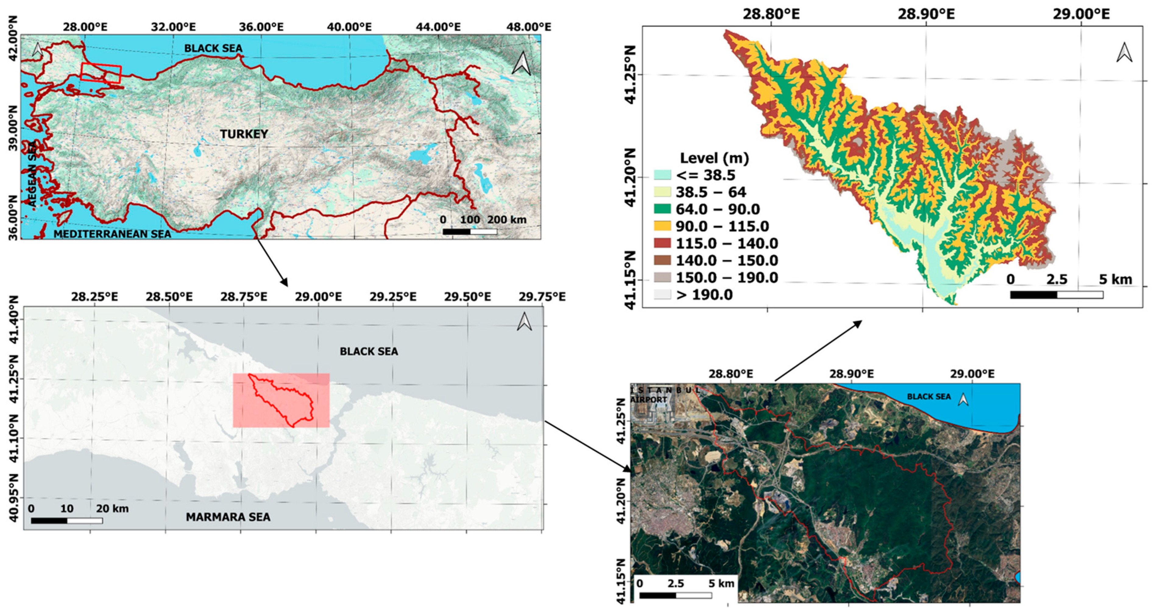
Figure 1. Location and topography of the study area.
Sustainability 17 10690 g001
Figure 2. Satellite images used in the study.
Sustainability 17 10690 g002
Figure 3. Land cover classification flowchart.
Sustainability 17 10690 g003
Figure 4. LULC prediction process with MOLUSCE.
Sustainability 17 10690 g004
Figure 5. Distance from creek.
Sustainability 17 10690 g005
Figure 6. Distance from road.
Sustainability 17 10690 g006
Figure 7. Digital elevation model.
Sustainability 17 10690 g007
Figure 8. Aspect map.
Sustainability 17 10690 g008
Figure 9. Slope map.
Sustainability 17 10690 g009
Figure 10. Population density.
Sustainability 17 10690 g010
Figure 11. Land cover categories for the year 2017.
Sustainability 17 10690 g011
Figure 12. Land cover categories for the year 2020.
Sustainability 17 10690 g012
Figure 13. Land cover categories for the year 2023.
Sustainability 17 10690 g013
Figure 14. Land use spatial distribution.
Sustainability 17 10690 g014
Figure 15. Land cover change between 2017 and 2020.
Sustainability 17 10690 g015
Figure 16. Land cover change between 2020 and 2023.
Sustainability 17 10690 g016
Figure 17. Land cover change between 2017 and 2023.
Sustainability 17 10690 g017
Figure 18. Predicted land cover classes for 2035, 2050, 2065, 2080, and 2095.
Sustainability 17 10690 g018
Figure 19. Changes in predicted land cover classes for 2035, 2050, 2065, 2080, and 2095 relative to 2023.
Sustainability 17 10690 g019aSustainability 17 10690 g019b
Figure 20. Total carbon emission (sum of direct and indirect carbon emission) with land use change.
Sustainability 17 10690 g020
Table 1. Sentinel-2 MSI satellite bands and their characteristics.
BandPixel SizeWavelengthDescription
B160 m443.9 nm (S2A)/442.3 nm (S2B)Aerosols
B210 m496.6 nm (S2A)/492.1 nm (S2B)Blue
B310 m560 nm (S2A)/559 nm (S2B)Green
B410 m664.5 nm (S2A)/665 nm (S2B)Red
B520 m703.9 nm (S2A)/703.8 nm (S2B)Red Edge 1
B620 m740.2 nm (S2A)/739.1 nm (S2B)Red Edge 2
B720 m782.5 nm (S2A)/779.7 nm (S2B)Red Edge 3
B810 m835.1 nm (S2A)/833 nm (S2B)NIR
B8A20 m864.8 nm (S2A)/864 nm (S2B)Red Edge 4
B960 m945 nm (S2A)/943.2 nm (S2B)Water vapor
B1120 m1613.7 nm (S2A)/1610.4 nm (S2B)SWIR 1
B1220 m2202.4 nm (S2A)/2185.7 nm (S2B)SWIR 2
Table 2. Producer’s and user accuracies for classification by year.
Class201720202023
UDPAUDPAUDPA
Built-up1.0000.9840.9691.0000.9840.954
Vegetation1.0000.9541.0000.9711.0000.955
Forest0.9661.0001.0001.0000.9861.000
Bare fields0.9850.9700.9550.9550.9211.000
Water bodies1.0001.00000.9841.0001.0001.000
Roads0.9631.0001.0000.9840.9850.970
Table 3. Transition matrix from 2017 to 2020.
2020
2017 Built-upVegetationForestBare FieldWater BodyRoads
Built-up61.6%18.5%0.2%7.9%0.1%11.8%
Vegetation10.3%75.9%3.6%6.6%0.1%3.5%
Forest0.3%5.6%93.4%0.5%0.1%0.2%
Bare field8.8%24.0%0.0%48.9%2.6%15.6%
Water Body1.4%2.0%2.1%2.1%87.7%4.7%
Roads11.2%9.5%0.0%12.2%0.5%66.5%
Table 4. Transition matrix from 2020 to 2023.
2023
2020 Built-upVegetationForestBare FieldWater BodyRoads
Built-up64.2%23.4%0.8%8.0%0.0%3.5%
Vegetation7.2%72.1%14.8%4.7%0.0%1.2%
Forest0.1%1.8%97.8%0.2%0.0%0.0%
Bare field13.6%15.9%0.0%64.8%0.5%5.2%
Water Body0.8%3.0%5.6%2.4%83.5%4.8%
Roads25.1%7.7%0.2%11.4%0.3%55.2%
Table 5. Transition matrix from 2017 to 2023.
2023
2017 Built-upVegetationForestBare FieldWater BodyRoads
Built-up62.7%21.5%0.6%8.8%0.1%6.4%
Vegetation11.9%70.5%7.2%8.3%0.1%2.0%
Forest0.3%4.6%94.1%0.7%0.1%0.2%
Bare field12.3%29.1%0.3%46.6%2.8%9.0%
Water Body1.4%5.1%4.5%3.8%78.3%6.8%
Roads24.9%9.9%0.2%15.4%0.4%49.2%
Table 6. Combinations of driving (spatial variable) factors.
Spatial Variable (Driving) FactorsScenarios
S1S2S3S4S5
Population DensityXX
Distance from the CreeksX XX
Distance from the RoadsXX X
Digital Elevation ModelXXXXX
AspectX X
SlopeX X
Table 7. Kappa values based on combinations of driving factors.
Scenarios Name% Kappa CorrectnessKappa (Overall) CoefficientsKappa (Histo) CoefficientsKappa (loc) Coefficients
S191.88500.84200.90360.9319
S286.96750.74510.89320.8342
S386.16780.73180.88980.8224
S487.17690.74820.92180.8116
S586.37840.73430.88340.8313
Disclaimer/Publisher’s Note: The statements, opinions and data contained in all publications are solely those of the individual author(s) and contributor(s) and not of MDPI and/or the editor(s). MDPI and/or the editor(s) disclaim responsibility for any injury to people or property resulting from any ideas, methods, instructions or products referred to in the content.