Experimental Evaluation of Feedback Proportional–Integral Control for Improving the Efficiency and Sustainability of DFIG Systems in Renewable Energy Applications

Abstract

This study investigates the effectiveness of a feedback-based proportional–integral (PI) regulator in the control system of a doubly fed induction generator (DFIG) used in wind energy applications, with a focus on enhancing the reliability and sustainability of renewable power generation. The primary objective is to assess how the feedback-based PI regulator can improve the efficiency and stability of rotor-side converter control, thereby ensuring consistent power quality and resilient operation under variable environmental and loading conditions. A novel experimental setup was developed by integrating a laboratory-scale DFIG system with real-time digital simulation tools, enabling a realistic assessment of dynamic performance. Various operating scenarios, including wind speed fluctuations and generator parameter variations, were analyzed to evaluate the regulator’s ability to minimize power ripples, ensure voltage stability, reduce total harmonic distortion (THD), and mitigate torque ripple—all of which contribute to more sustainable and efficient energy conversion. Comparative analyses using performance indicators such as power ripple, steady-state error, and overshoot demonstrate that the feedback-based PI regulator outperforms conventional control methods reported in the literature. The experimental results confirm that the proposed control strategy not only enhances dynamic performance and operational robustness but also contributes to the long-term sustainability of wind energy systems by improving energy efficiency, reducing losses, and supporting grid stability. Overall, this work promotes sustainability by advancing control techniques that optimize renewable energy utilization and strengthen the reliability of clean power technologies.

1. Introduction

Doubly fed induction generators (DFIGs) are extensively employed in wind energy (WE) systems, a practice that can be attributed to their capacity to function over a broad spectrum of wind speeds (WSs) [1]. In these generators, reactive and active powers (Qs and Ps) are regulated independently. In DFIGs, sub-scale power converters are employed, offering a cost-effective and efficient solution [2]. The distinguishing characteristics of the DFIG generator that set it apart from other types include its low maintenance requirements, high strength, ease of command, and the ability to regulate the rotor feed, thereby modulating the output energy [3]. The aforementioned features of the DFIG generator render it an optimal solution for the control system that is the focus of this paper.

The primary objective of DFIG command methodologies is to optimize energy capture, ensure adherence to grid regulations, and safeguard the system. A number of control algorithms have been developed to enhance the power output of DFIGs. The proportional–integral (PI) regulator is frequently employed for power control [4,5]. Its advantages make it a compelling solution. As illustrated in

Table 1. Key control approaches for DFIGs.

Controls	Description	Implementation	Benefits	Limitations
Field-oriented control (FOC) [6]	Separates control of DFIG power using decoupled control of the stator flux and rotor current in a rotating d–q reference frame.	Typically, stator flux orientation is used.	Decoupled command of torque and flux. Fast dynamic response. Good for grid integration.	Sensitive to parameter variations (e.g., rotor resistance). Requires accurate machine modeling and coordinate transformation.
Model predictive control (MPC) [7]	Uses a predictive model of the DFIG to compute control actions that minimize a cost function over a prediction horizon.	-	Handles constraints (voltage, current). Good dynamic performance.	High computational complexity. Sensitive to model inaccuracies. Not widely implemented in commercial turbines due to real-time hardware limitations.
Sliding mode command (SMC) [8,9]	A robust nonlinear command algorithm that forces system dynamics to “slide” along a predefined surface.	-	Robust to parameter variations and disturbances.	Chattering phenomenon (high-frequency oscillations). Complex implementation and tuning.
Direct power control (DPC) [10]	Controls the DFIG energy directly without using inner current loops or coordinate transformation.	Based on the instantaneous power theory; uses a switching table.	Fast dynamic response. Simpler control structure (no PI regulators or decoupling loops).	Higher torque and current ripple. Difficult to implement with fixed switching frequency. Needs fast switching devices.
PI control with decoupling [11]	Classic PI regulators used in the current command loops, often with decoupling terms to account for cross-coupling between d- and q-axes.	-	Simplicity and ease of implementation.	Slower dynamic response compared to advanced methods. Tuning is sensitive to system operating conditions.

, the following control algorithms are employed to regulate DFIG power, along with their salient limitations.

Conventionally, the DPC approach has been the most prevalent algorithm in the domain of renewable energy, particularly WE [12]. This algorithm is regarded as one of the most prevalent solutions for power control in DFIG. The implementation of DPC facilitates the efficient and effective regulation of power flow between the electrical grid and the stator of the DFIG. This is achieved by directly regulating the DFIG energy of the stator via a rotor-side converter (RSC), obviating the necessity for coordinates transformations or internal current control loops, which are essential in conventional control methodologies [13]. Furthermore, the DPC strategy has been demonstrated to be a rapid method that does not require precise data of the energy system model under consideration, thereby making it a suitable and reliable solution [14,15].

The fundamental principle of DPC strategy entails the selection of suitable switching states for the power converter, contingent on the instantaneous errors in DFIG energy [16]. This objective is accomplished by implementing a hysteresis-based control scheme and a switching schedule derived from the DFIG power model in the stator flux reference frame. Consequently, the utilization of the DPC technique ensures a rapid and adaptable response, a reduction in complexity, and an effective rejection of disturbances. This renders it particularly well-suited for WE applications, where the ability to swiftly adapt to changing wind conditions is paramount [17]. As indicated in the research conducted in [18], the DPC strategy was employed to regulate a synchronous generator. The obtained results demonstrated the efficacy of this algorithm in enhancing the performance of the studied system. In addition, the DPC yielded satisfactory results in operation [19] when compared to the FOC with regard to current fluctuations and powers. Additionally, the DPC technique yielded a superior performance in terms of total harmonic distortion (THD) when compared to the FOC strategy. Notwithstanding the merits of the DPC approach, it is subject to certain drawbacks, including variable switching frequency and power fluctuations [20]. To address these limitations, enhanced and adapted DPC techniques have been developed, encompassing predictive and vector-space-based methodologies [21]. In [22], the utilization of neural networks was put forth as a methodology to enhance the features of the DPC. The use of neural networks has significantly improved the robustness and performance of the DPC. However, using neural networks allows for a significantly higher level of complexity in the DPC compared to the traditional approach. Furthermore, neural network algorithms rely heavily on experimentation and experience to achieve good results, which requires considerable time and effort. Another solution adopted in work [23] to overcome the problem of poor power quality (PQ) when using the DPC strategy in a DFIG-based system is to use a backstepping controller (BC) to replace traditional controllers. Also, pulse width modulation (PWM) was used to compensate for the use of a switching table. The employment of a BC method has been demonstrated to enhance the THD value and mitigate power ripples when compared to conventional algorithms. This approach has also been shown to reduce overshoot and steady-state error (SSE). Despite the efficacy of employing a BC method, numerous challenges persist, the most salient of which pertains to the considerable complexity, which renders the developed approach experimentally costly. Furthermore, the presence of numerous gains complicates the adjustment and modification of this developed approach. Fractional-order proportional–integral (FOPID) control was suggested in the work [24] using the Grey-Wolf optimization (GWO) algorithm for power control (DFIG). This approach builds upon the usual strategy, where PWM is used to command the operation of the RSC. This command method was simulated using MATLAB (2014)/Simulink, and its performance was compared to that of a standard PI. The results obtained show that the THD in the rotor current was 2.55%, while the THD in the suggested methods, using an FOPID optimization tool and a standard PI, was 6.21% and 8.67%, respectively. The results achieved using the new GWO-FOPID are superior to those achieved using an FOPID tuned with an FPID optimization tool and a standard PI. In the study [25], neural networks were designed as a suitable solution to overcome the problems of the DPC approach, where the dual MLP approach was used to precisely regulate power. This algorithm was compared with both the classical algorithm and DPC-PI using simulation and a real-time simulator (OPAL-RT). The results indicate that the designed approach yielded a THD of current of 1.29%, while the DPC-PI approach yielded values of 2.76% and 2.24%, respectively, when using the DPC-classic strategy. Furthermore, the results indicate that the designed approach yielded a 78.70% and 34.19% better standard deviation for Ps compared to the usual algorithm. In terms of precision, the approach demonstrates high accuracy compared to other algorithms. Despite its high performance, this algorithm has drawbacks, including observed fluctuations in both current and power output. Furthermore, its complexity is a major disadvantage, making it experimentally costly. Work [26] addresses a critical challenge in WE systems by developing a DPC strategy for a DFIG-type generator operating under unbalanced grid voltage conditions. In this work, a control scheme is formulated that regulates both Ps and Qs, despite the negative sequence voltage components that typically arise during grid imbalance. This tailored control method helps curb harmful dual-frequency fluctuations in torque and power, which degrade generator performance, thereby enhancing system stability and PQ. Through precise rotor-side transformer control design, imbalances are compensated for without excessive complexity, making this approach particularly valuable for wind turbines susceptible to grid disturbances.

In [27], the voltage modulated DPC was designed as an alternative to the classical approach for power command in DFIG. This strategy is an improvement on the traditional method, offering satisfactory performance compared to the classical algorithm. This technique relies on the introduction of a modulated voltage for the Ps and Qs and a nonlinear power control unit, which allows the generator dynamics to shift from time-varying differential equations to time-constant equations. This strategy was implemented in MATLAB (2014) under balanced grid voltage conditions. Simulation results demonstrate the effectiveness of the developed strategy compared to the traditional algorithm in terms of torque, power, and current ripples. Furthermore, it significantly reduces the THD of both rotor and stator currents. Among the most prominent solutions proposed for power control is the FOPID controller based on the Root Tree Optimization (RTO) algorithm [28]. This regulator is characterized by high performance and robustness due to the use of the RTO algorithm in determining gains. As is well known, the use of intelligent algorithms allows for increased operational performance and significantly improved current and PQ. This designed solution was compared with the PI controller using MATLAB (2014), and the results showed high efficiency and effectiveness in improving the characteristics of the studied power system. However, in the durability test, it was observed that this designed regulator was significantly affected by changes in the machine parameters, resulting in greater power fluctuations. Furthermore, the presence of a significant number of potential gains makes determining optimal gain values time-consuming. Using smart strategies does not always yield good results, especially with newer strategies like RTO, which necessitate repeatedly calculating optimal values, thus making the process of determining optimal gains cumbersome. In [29], the author replaced the traditional DPC of DFIG with a second-order SMC approach. This approach does not rely on a switching table, making it entirely different from the traditional technique. This approach was implemented only on the machine’s inverter. It was implemented in MATLAB (2014) using the variable WS. Furthermore, this approach was tested in terms of changing DFIG parameters. Compared to the PI regulator, the designed solution yielded highly satisfactory results in terms of reducing current and torque ripple. Furthermore, this solution boasts high robustness and a significant ability to reduce the current THD. Its main drawbacks are its complexity and the number of gains. Additionally, its reliance on power estimation leads to performance degradation if the machine parameters change. In [30], RST, sliding mode technique, and fuzzy supervisory controllers were proposed as viable and reliable solutions for power control in DFIG. These solutions were compared with the PI using MATLAB (2014). The use of these solutions significantly improves performance in terms of energy fluctuation and response time, as well as robustness, and reduces the current THD. These solutions are characterized by a higher degree of complexity compared to the PI controller. Adaptive-gain second-order sliding mode DPC technique is a work-designed solution [31] to replace the traditional power command strategy for DFIG. This approach is characterized by greater complexity and a higher gain. The strategy was implemented on a 2 MW generator using MATLAB (2014) under various operating conditions. The new algorithm achieved DFIG energy regulation under a two-phase stationary reference frame for both balanced and unbalanced grid voltage. An uncertainty upper bound is not needed in advance, and the SMC chattering is greatly restrained. The results verify the robustness, effectiveness, and superiority of the suggested method. In [32], the use of RST and active disturbance rejection command algorithms was proposed as a possible solution to improve the PQ of a system based on a DFIG-type generator. The performance of these solutions was compared to that of a PI under varying wind conditions, using MATLAB (2014) for this purpose. These solutions differ significantly from the PI regulator and other methods, such as SMC, in terms of performance, simplicity, robustness, and ease of implementation. Simulation results demonstrate the ability of these strategies to improve current and power quality compared to the PI regulator. Despite their effectiveness, the degree of complexity is one of the major challenges hindering the widespread adoption of these solutions in the field of control. A matrix converter was used in work [33] to overcome the shortcomings of the DPC strategy of DFIG. Indirect space vector modulation was used to control the matrix converter. This approach was compared with the traditional strategy in terms of performance, reference tracking, robustness, and PQ. The simulation results from the MATLAB (2014) environment demonstrated the effectiveness and efficiency of this approach in improving power and current quality compared to traditional methods. However, the difficulty and complexity of implementation are among the most significant drawbacks of this approach, making its application in the renewable energy sector costly. In [34], the utilization of SMC was conceived to augment the efficacy of the DPC of DFIG. The outcomes substantiate the efficacy of employing SMC and its capacity to enhance the properties of the DPC method. This enhancement is discernible in the mitigation of torque and current fluctuations in comparison to the DPC. However, the implementation of SMC renders the DPC approach contingent on the generator parameters, thereby leading to a diminution in PQ in the event of a change in the resistance of the rotor or stator coils. Additionally, the implementation of SMC gives rise to a chattering problem, which in turn affects the efficacy of the command system. Overall, the DPC strategy remains a compelling approach for DFIG, primarily due to its simplicity, clarity, and performance in dynamic environments. This algorithm is a reliable tool in the field of control, aiming to develop more efficient solutions while preserving simplicity and ease of realization.

In the domain of control systems, the feedback proportional–integral (FPI) controller has emerged as a leading solution, exhibiting superior efficiency in comparison to the conventional PI, as documented in [35]. The merits of this regulator are manifold, including its rapid dynamic response, ease of adjustment, simplicity of implementation, and low cost. Moreover, its use does not necessitate precise data of the system under study. In [36], a PI regulator based on a GA was implemented in a DPC-PWM scheme and validated via in-loop processor tests, demonstrating a significant reduction in energy ripple and THD. However, the work does not include a detailed analysis of the Lyapunov’s closed-loop stability, nor extensive experiments on real-world devices across low- and high-speed regimes under varying parameters. In the study [37], an FPI regulator was proposed under direct vector control and validated only via MATLAB (2014) simulation, again without explicit proof by Lyapunov’s theorem or full experimental verification.

Although many studies have explored optimization controllers using GA or FPI algorithms for DFIG systems, most have been limited to simulation implementations and have not investigated stability. In this work, we propose a feedback method-based GA-PI regulator that incorporates a dynamic feedback mechanism within the GA algorithm optimization loop, relying on experimental validation using real instruments. Using the GA strategy allows for the identification of optimal gain values, which greatly improve durability and dynamic response under different operating conditions. Furthermore, this study expands upon previous work by incorporating stability analysis using Lyapunov’s theory. These combined improvements establish the proposed method as a novel and practical enhancement to existing FPI-based DFIG control approaches.

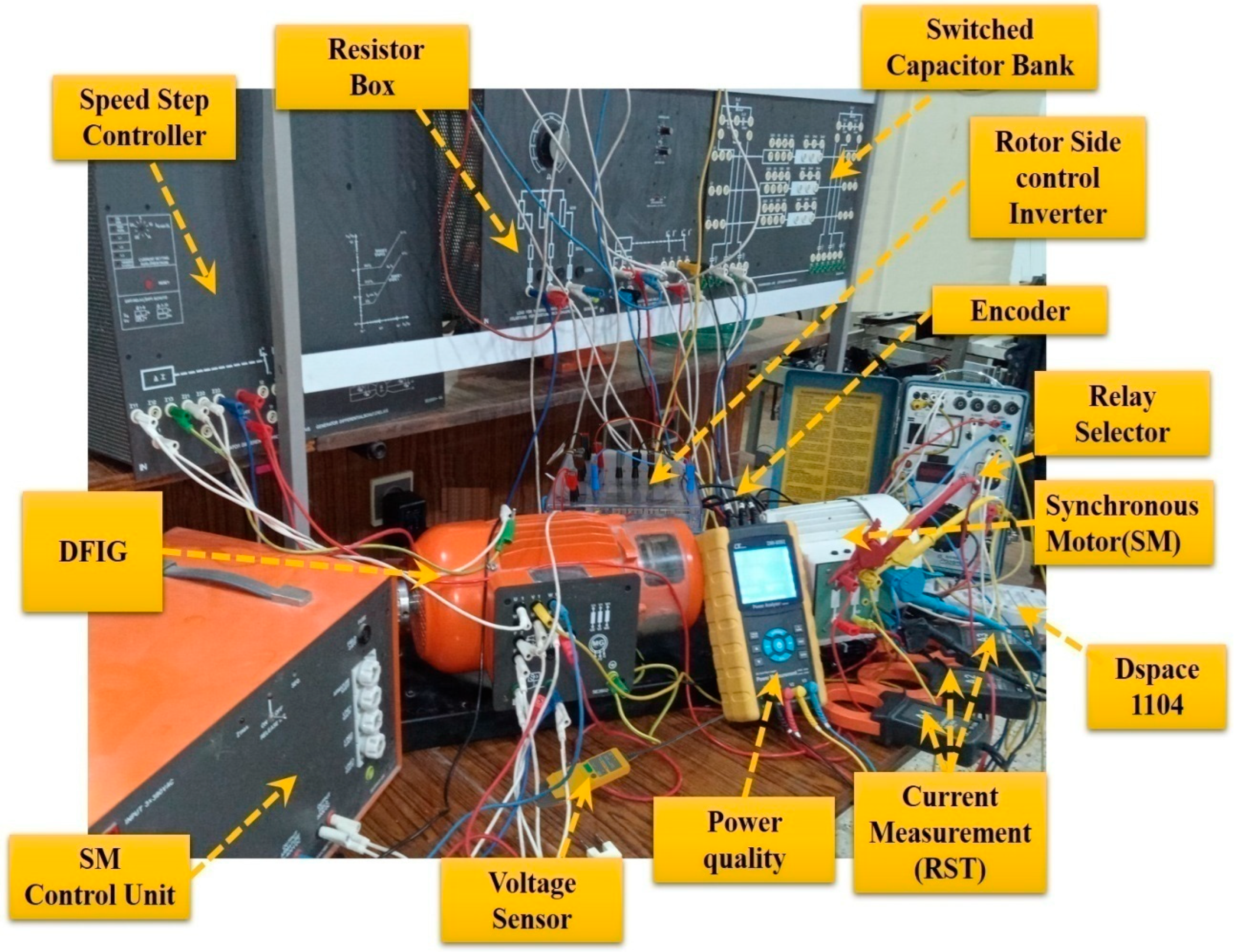
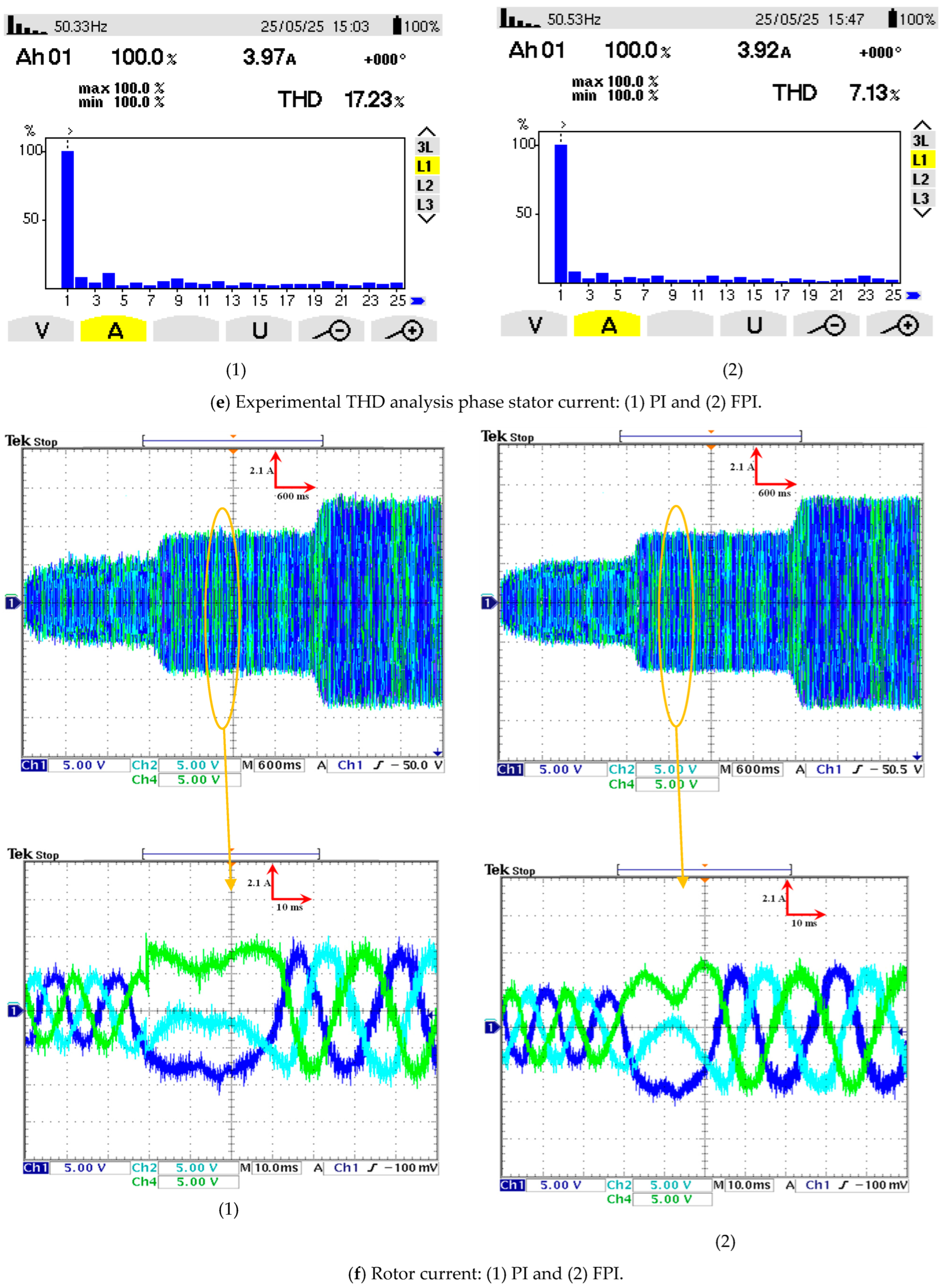
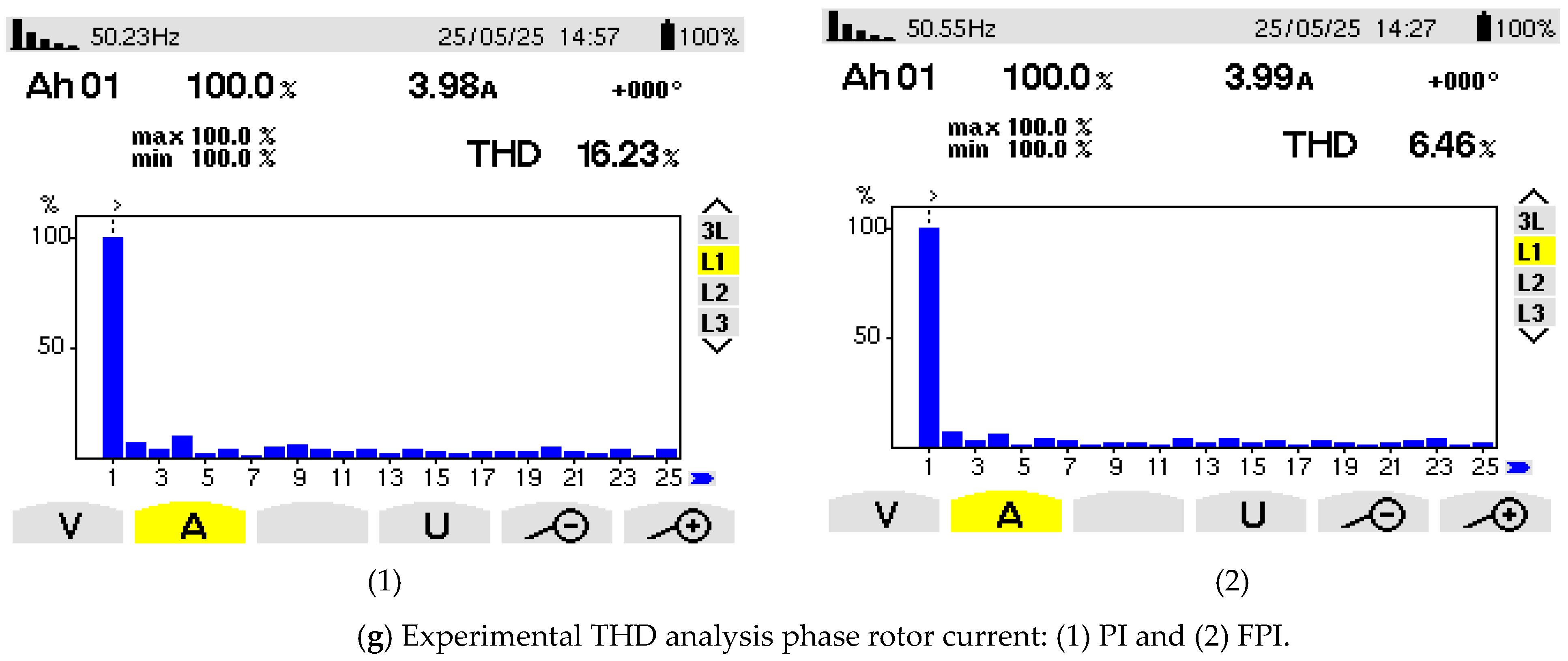
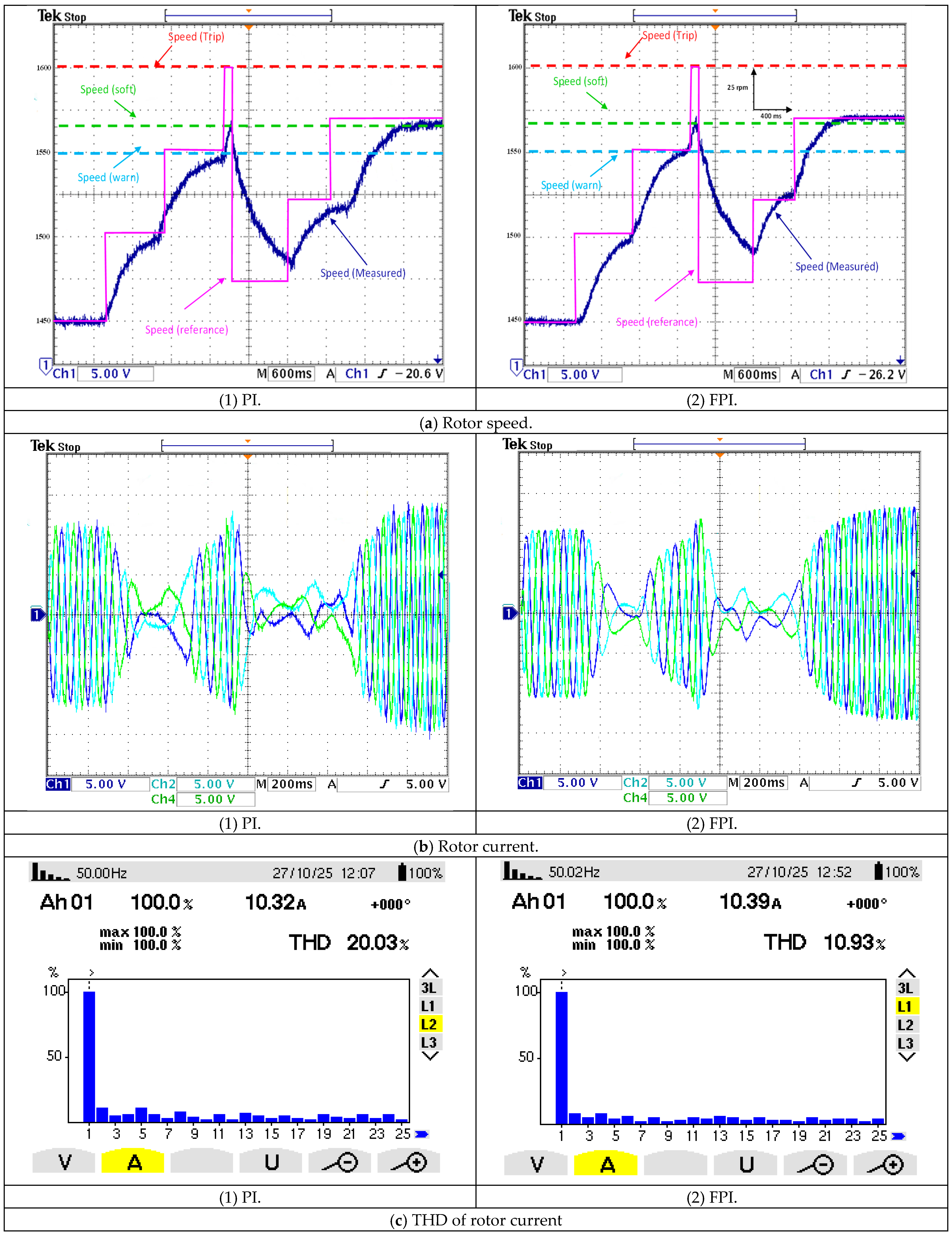
In contrast, this manuscript (i) presents a genetically optimized FPI regulator with Lyapunov’s-based stability proof, (ii) applies it to real devices covering operation at low and high speeds and in the case of cut-in and cut-out speeds, (iii) compares DPC-PI-based constructs under identical device tests, (iv) reports the measured THD and ripple values (e.g., THD = 6.34% at low speed, THD = 0.56% at high speed), demonstrating the practical feasibility of this approach. This contribution thus expands the scope of cutting-edge techniques in ensuring both theoretical stability and practical experimental verification. The mathematical modeling of the FPI is presented first, highlighting its main drawbacks. The approach designed for power control is applied to the RSC only to demonstrate its effectiveness and power in improving PQ without resorting to grid inverter control. The effectiveness of the FPI is first verified through MATLAB (2014) simulations under various operating conditions (e.g., at cut-in and cut-out speeds). The next phase involves experimental implementation using real-world instruments for this designed approach. In this experimental work, dSPACE 1104 is used to demonstrate the proposed approach. The effectiveness of this designed command is evaluated compared to the PI controller in terms of robustness, PQ, overshoot, and SSE value. Furthermore, a comparison with relevant works is conducted to highlight the effectiveness and efficiency of this approach. This experimental work is of great importance in the energy field, as it provides a more effective solution in terms of simplicity, operational performance, durability, and ease of application and completion.

This experimental work stands out for its clear departure from previous studies in this field, underscoring its significance in energy research. Table 2 provides a comparison with related works, highlighting the differences between this study and some existing research. The experimental results largely confirm the simulation findings, demonstrating the effectiveness of the FPI regulator in improving power characteristics. The following points outline the main objectives achieved by this study.

• Accurate tracking of the energy reference.
• Maintaining the reactive power at the required setpoint, this has been set to zero (for a single power factor).
• Independent control of the Qs and Ps of the DFIG.
• Simplified design and improved dynamic response.
• Smoother power output and improved quality.
• The feedback action feature in the PI controller ensures no errors in stability when tracking Ps and Qs references.
• The designed approach promotes sustainability by developing control technologies that optimize the use of renewable energy.
• Enhancing the reliability of clean energy technologies.
• Reduced overshoot, faster settling time.
• Stable performance under model uncertainties.
• Higher efficiency, compliance with power-quality standards (e.g., IEEE 519) [38].
• PI controllers integrate seamlessly with PWM converters for continuous and smooth switching control.
• Obtain a more effective regulator for industrial applications and real-time systems.

Table 2. Comparing the completed work with the work [36,37].

Performances	Works
	[36]	[37]	Proposed Works
Robustness study	Yes: the effect of changing generator parameters (parametric variation) was studied for robustness.	Durability was studied in the face of changes in WS.	Yes: The effect of changing the generator parameters (parametric variance) was studied to verify its robustness. Additionally, the regulator’s effectiveness was tested under cut-in and cut-out speed conditions.
Stability study	Stability has not been studied using Lyapunov’s theory. This study relies primarily on simulation.	The stability performance using Lyapunov’s theory has not been studied.	Yes, stability has been proven using Lyapunov’s theory.
Experimental vs. Simulation	Simulation only (MATLAB (2014)) over various operating conditions.	Mixed: They do simulation and also “processor-in-the-loop (PIL)” tests (dSPACE 1104) for the DPC-GA-PI scheme.	Mixed: Simulation and experimental work were also carried out using real instruments.
THD/current quality reported	Numerical results were extracted from the simulation, including the THD of the current and SSE/overshoot.	They report, e.g., current THD reductions: “the current THD value was minimized by high ratios (72.88%, 45.45%, and 78.18%) in the two experimental tests.”	The numerical simulation results, including the THD of the current, SSE/overshoot, and power ripples, were extracted. The THD value at variable WS was estimated to be 1.22% when using the FPI regulator.
Tests at low & high speeds	Various different operating conditions were studied, including parameter variations, but precise low (3 m/s) and high (25 m/s) speed regimes were not studied.	The tests are conducted under “various operating conditions,” including varying WSs. A study at cut-in and cut-out speeds has not yet been completed.	The designed approach was tested under varying WS conditions and in increments. It was also tested under cut-in and cut-out WS conditions.
Control type	Feedback PI controller used in a direct vector control (DVC) scheme of DPAG (double-powered asynchronous generator) with a two-level PWM inverter.	GA-tuned PI controller inside a DPC scheme (with PWM) for a variable-speed contra-rotating wind turbine (DFIG) system.	Feedback PI controller used in a DPC scheme of DFIG

Table 2. Comparing the completed work with the work [36,37].

Performances	Works
	[36]	[37]	Proposed Works
Robustness study	Yes: the effect of changing generator parameters (parametric variation) was studied for robustness.	Durability was studied in the face of changes in WS.	Yes: The effect of changing the generator parameters (parametric variance) was studied to verify its robustness. Additionally, the regulator’s effectiveness was tested under cut-in and cut-out speed conditions.
Stability study	Stability has not been studied using Lyapunov’s theory. This study relies primarily on simulation.	The stability performance using Lyapunov’s theory has not been studied.	Yes, stability has been proven using Lyapunov’s theory.
Experimental vs. Simulation	Simulation only (MATLAB (2014)) over various operating conditions.	Mixed: They do simulation and also “processor-in-the-loop (PIL)” tests (dSPACE 1104) for the DPC-GA-PI scheme.	Mixed: Simulation and experimental work were also carried out using real instruments.
THD/current quality reported	Numerical results were extracted from the simulation, including the THD of the current and SSE/overshoot.	They report, e.g., current THD reductions: “the current THD value was minimized by high ratios (72.88%, 45.45%, and 78.18%) in the two experimental tests.”	The numerical simulation results, including the THD of the current, SSE/overshoot, and power ripples, were extracted. The THD value at variable WS was estimated to be 1.22% when using the FPI regulator.
Tests at low & high speeds	Various different operating conditions were studied, including parameter variations, but precise low (3 m/s) and high (25 m/s) speed regimes were not studied.	The tests are conducted under “various operating conditions,” including varying WSs. A study at cut-in and cut-out speeds has not yet been completed.	The designed approach was tested under varying WS conditions and in increments. It was also tested under cut-in and cut-out WS conditions.
Control type	Feedback PI controller used in a direct vector control (DVC) scheme of DPAG (double-powered asynchronous generator) with a two-level PWM inverter.	GA-tuned PI controller inside a DPC scheme (with PWM) for a variable-speed contra-rotating wind turbine (DFIG) system.	Feedback PI controller used in a DPC scheme of DFIG

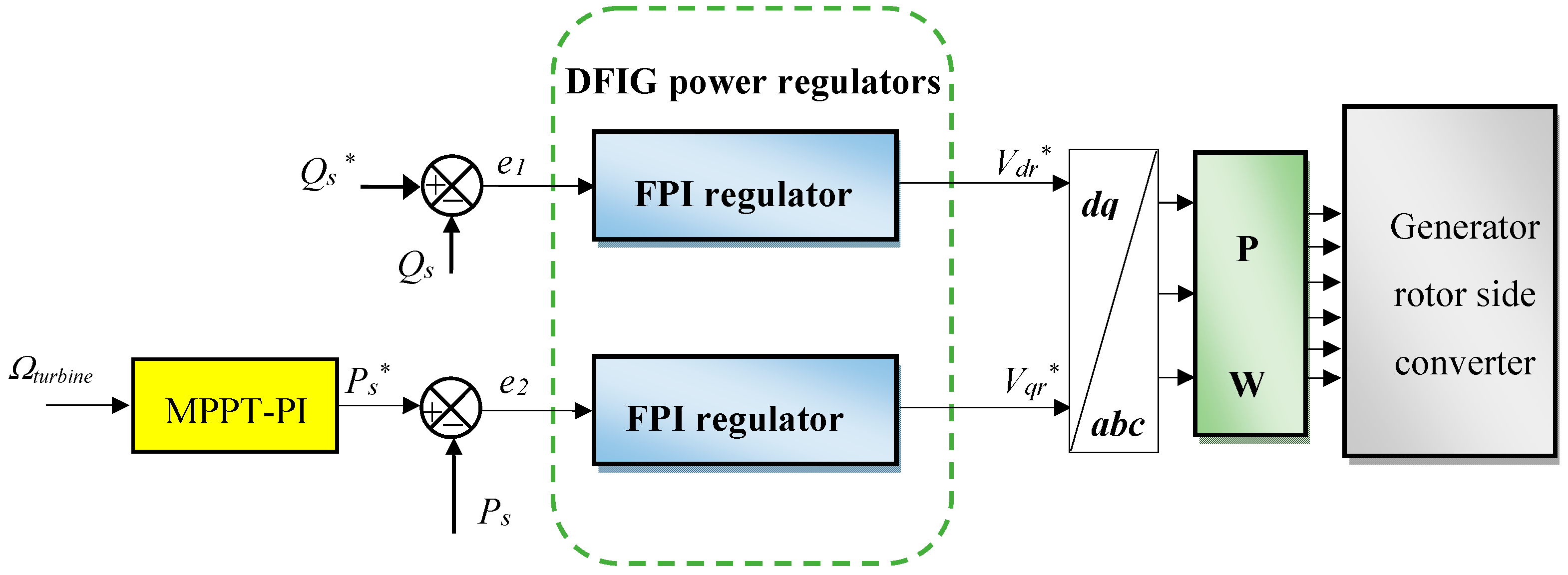
The paper is divided into five sections. The Section 2 of this study will focus on the FPI regulator and its primary advantages. The Section 3 of this study will address the application of the FPI regulator for controlling DFIG power. The Section 4 employs the MATLAB 2014 software to assess the efficacy of the FPI regulator. The Section 5 is devoted to an experimental examination of the FPI regulator, utilizing authentic instruments to assess its performance in comparison to that of a PI regulator. In conclusion, the findings of this study are outlined in Section 6.

2. FPI Controller

A PI is a feedback control mechanism that has found wide application in the domains of process control and industrial control systems [39]. This unit integrates two fundamental control functions: an integral component that manages the accumulation of past errors and a proportional component that responds to the current error [40]. Collectively, these functions assist the controller in maintaining the desired setpoint and minimizing SEE [41].

In contrast to the PID controller, the PI controller does not incorporate a derivative term, a feature that contributes to its enhanced stability in noisy environments [42]. PI controllers are valued for their simplicity, effectiveness, and ease of realization in many applications, including pressure systems, temperature regulation, and motor speed control [43].

Mathematically, the PI can be expressed as follows:

$${y\left(t\right)=K}_1.e\left(t\right)+K_2.\int e\left(t\right)dt$$

(1)

where y(t) is the PI output and e(t) is the error.

Despite the widespread use of the PI, this controller faces several limitations, especially in complex or time-varying systems. Key challenges include poor performance with nonlinear or time-varying systems, integral windup, limited adaptability, and sensitivity to noise and disturbances [44].

In order to surmount these challenges, a series of improvements and strategies has been advanced. The most prominent of these solutions involves the use of intelligent strategies, including neural networks [45] and fuzzy logic [46]. In a similar vein, SMC and backstepping control strategies have been put forth as effective solutions to replace the use of PI regulators in control [47,48]. The efficacy of these strategies is evident in their high degree of robustness and satisfactory operational performance. Nevertheless, the implementation of these systems invariably increases the complexity of the process, which in turn results in higher implementation costs. Consequently, the quest for a substitute for PI controllers is of the utmost importance, with a focus on simplicity, ease of application, and ease of control. A comprehensive review of the extant literature reveals that the FPI regulator is regarded as a promising and reliable control solution that has the potential to supplant the utilization of PI regulators. This regulator represents advancement in the field, evolving from the PI regulator. Its salient features include simplicity, ease of adjustment, and implementation. In addition, the regulator’s performance characteristics, including its operational effectiveness and durability, set it apart from numerous conventional models.

As indicated in the research conducted in [37], the FPI regulator is expressed by Equation (2).

$${u\left(t\right)=K}_1.e\left(t\right)+K_2.\int E\left(t\right)dt$$

(2)

with

$$E\left(t\right)=e\left(t\right)-K_3.h\left(t\right)$$

(3)

$$h\left(t\right)=K_2.\int E\left(t\right)dt$$

(4)

Substitution of Equation (3) into Equation (2) results in the expression of Equation (5), which represents the final form of the FPI regulator.

$${u\left(t\right)=K}_1.e\left(t\right)+K_2.\int e\left(t\right)dt-K_2.K_3\int h\left(t\right).dt$$

(5)

where $u\left(t\right)$ is the output of the FPI regulator.

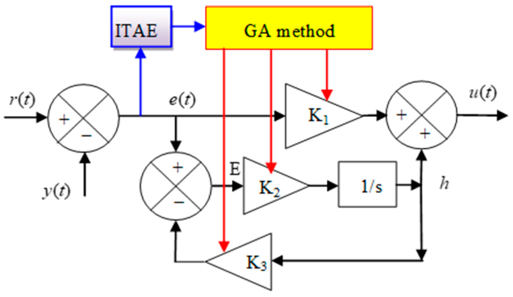
K₁, K₂, and K₃ are the regulator gains. These values are used to change the dynamic response. In this controller, K₃ can be set to 1 to facilitate adjustment and modification of the dynamic response. These gains are calculated using a GA. Using this algorithm significantly improves performance and enhances robustness. This algorithm was chosen for its ease of use and the fact that it does not require writing complex programs; the gatool is used for this purpose. The Integral of Time multiplied by Absolute Error (ITAE) is used to determine the optimal gain values. The algorithm’s characteristics are detailed in the Supplementary Materials.

As illustrated in Figure 1, the controller enumerated in Equation (5) can be conceptualized as follows:

The values of the designed controller’s gains can be calculated using simulation and experimentation. The calculation of these gains can be facilitated through the implementation of intelligent algorithms, such as the GA technique. This algorithm is characterized by its reliability in determining optimal gain values, a property that is attributable to its ease of use.

Table 3. Comparison of FPI with some existing regulators in the literature.

Controllers	Ripple Sppression	THD Minimization	Dynamic Response	Robustness to Uncertainty	Chattering	Implementation Complexity	Computational Load
FPI	Moderate-high	Moderate–high	Fast	Moderate	None	Low–moderate	Low
SMC	High	High	Very fast	Very high	High	Moderate	Moderate
PI	Moderate	Moderate	Moderate	Low	None	Very low	Very low
STA	High	High	Very fast	Very high	None	High	Moderate
Backstepping controller	High	High	Good	High	None	High	High
Synergetic controller	High	High	Fast	High	None	High	High
Model predictive controller	Very high	Very high	Excellent	High	None	Very high	Very high

compares the FPI with some existing regulators in the literature in terms of performance and characteristics. This table illustrates the similarities and differences between the suggested controller and some of these controllers. Table 3 demonstrates that the FPI controller is similar to synergetic controllers, STA controllers, backstepping controllers, and predictive control models in that it lacks chattering. Furthermore, the controller has a rapid dynamic response, similar to a synergetic controller. Table 3 shows that the computational overhead of the FPI controller is significantly lower than that of other controllers, such as synergetic controllers, SMC, STA, and backstepping controllers. However, in terms of robustness to uncertainty, the controller is less efficient than linear controllers such as SMC and backstepping controllers. In terms of complexity, the FPI is less complex than SMC, backstepping control, model predictive control, and STA, making it a reliable solution in the control field.

To demonstrate the stability of the FPI, it is possible to employ either Lyapunov’s theorem or Bode’s curve. In this paper, Lyapunov’s method is employed to derive stability conditions. The validity of this stability is substantiated by Equations (3)–(5).

Based on Equations (3) and (4), the following equation can be written as

$$E\left(t\right)=e\left(t\right)-K_3.K_3\int E\left(t\right).dt$$

(6)

Using the Laplace transform, Equation (3) can be written as

$$E\left(s\right)=e\left(s\right)-K_3.h\left(s\right)$$

(7)

Equation (4) becomes as follows:

$$h\left(s\right)=K_2.{\displaystyle \frac{1}{s}}E\left(s\right)={\displaystyle \frac{K_2}{s}}E(s)$$

(8)

By substituting Equation (8) into Equation (7), Equation (9) can be written as

$$E\left(s\right)=e\left(s\right)-K_3{\displaystyle \frac{K_2}{s}}E(s)$$

(9)

Equation (9) can be written as follows:

$$e\left(s\right)=E\left(s\right)(1+K_3{\displaystyle \frac{K_2}{s}})$$

(10)

From Equation (10) the expression E(s) can be extracted as follows:

$$E\left(s\right)={\displaystyle \frac{e\left(s\right)}{1+K_3\frac{K_2}{s}}}={\displaystyle \frac{s}{s+K_3{K}_2}}e(s)$$

(11)

Referring to Equation (2), this equation in the Laplace system is written as follows:

$${u\left(s\right)=K}_1.e\left(s\right)+K_2.\int E\left(s\right)dt$$

(12)

By substituting Equation (11) into Equation (12), the following equation is obtained:

$${u\left(s\right)=K}_1.e\left(s\right)+{\displaystyle \frac{K_2}{s}}{\displaystyle \frac{s}{s+K_3{K}_2}}e(s)$$

(13)

Equation (13) becomes as follows:

$${u\left(s\right)=[K}_1+{\displaystyle \frac{K_2}{s+K_3{K}_2}}]e(s)$$

(14)

Using a first-order system as listed in Equation (15).

$$Y\left(s\right)={\displaystyle \frac{b}{s+a}}U(s)$$

(15)

As we know, e(s) is an error. This error can be written according to Equation (16).

$$e\left(s\right)=R\left(s\right)-Y\left(s\right)$$

(16)

Using Equations (15) and (16), Equation (14) can also be written according to Equation (17).

$${u\left(s\right)=[K}_1+{\displaystyle \frac{K_2}{s+K_3{K}_2}}](e\left(s\right)-Y\left(s\right))$$

(17)

From Equation (17), we can write the following equation:

$${Y\left(s\right)={\displaystyle \frac{b}{s+a}}[K}_1+{\displaystyle \frac{K_2}{s+K_3{K}_2}}](R\left(s\right)-Y\left(s\right))$$

(18)

Simplify Equation (18) by assuming the existence of G(s) as shown in Equation (19).

$${G\left(s\right)=[K}_1+{\displaystyle \frac{K_2}{s+K_3{K}_2}}]$$

(19)

Therefore, Equation (18) becomes

$$Y\left(s\right)={\displaystyle \frac{b}{s+a}}.G\left(s\right).(R\left(s\right)-Y\left(s\right))$$

(20)

So

$$Y\left(s\right)[1+{\displaystyle \frac{b}{s+a}}.G\left(s\right)]={\displaystyle \frac{b.R\left(s\right)}{s+a}}.G\left(s\right)$$

(21)

Therefore, the equation that expresses the transfer function in the closed loop is as follows:

$${\displaystyle \frac{Y\left(s\right)}{R\left(s\right)}}={\displaystyle \frac{b.G\left(s\right)}{s+a+b.G\left(s\right)}}$$

(22)

From Equation (22), the following characteristic equation is extracted:

$$s+a+b.G\left(s\right)=0$$

(23)

Equation (23) can also be written as follows:

$$s+a+b.(K_1+{\displaystyle \frac{K_2}{s+K_3{K}_2}})=0$$

(24)

From Equation (24), the following can be written as

$$\left(s+K_3{K}_2\right)\left(s+a\right)+b.K_1\left(s+K_3{K}_2\right)+b{K}_2=0$$

(25)

Equation (25) becomes as follows:

$$s^2+s\left(a+K_3{K}_2\right)+a{K}_3{K}_2+b{K}_{1}s+b{K}_3{K}_2{K}_1+b{K}_2=0$$

(26)

Depending on the collection of terms, Equation (26) is written as follows:

$$s^2+s\left(a+K_3{K}_2+b{K}_1\right)+(a{K}_3{K}_2+b{K}_3{K}_2{K}_1+b{K}_2)=0$$

(27)

Equation (27) is written in the form $s^2+As+B=0$, with

$$\left\{\begin{array}{c}A=a+K_3{K}_2+b{K}_1\\ B=a{K}_3{K}_2+b{K}_3{K}_2{K}_1+b{K}_2\end{array}\right.$$

(28)

Equation (27) can be utilized to derive stability conditions for the designed regulator. For the system to be stable, it is necessary that both coefficients in Equation (28) be positive.

Therefore, the condition can be written as follows:

$$\left\{\begin{array}{c}A=a+K_3{K}_2+b{K}_1>0\\ B=a{K}_3{K}_2+b{K}_3{K}_2{K}_1+b{K}_2>0\end{array}\right.$$

(29)

The stability conditions can be extracted by assuming that a and b are positive. Therefore, the initial condition that can be extracted is shown in Equation (30).

$$K_1>-{\displaystyle \frac{a+K_3{K}_2}{b}}$$

(30)

The second condition that can be written is represented by Equation (31).

$$a{K}_3{K}_2+b{K}_3{K}_2{K}_1+b{K}_2>0$$

(31)

Equation (31) can also be written as follows:

$$K_2(a{K}_3+b{K}_3{K}_1+b)>0$$

(32)

So, $K_2>0$, and $a{K}_3+b{K}_3{K}_1+b>0$.

$$K_2(a{K}_3+b{K}_3{K}_1+b)>0$$

(33)

To extract a condition on K₃, Equation (34) is used.

$$a{K}_3+b{K}_3{K}_1+b>0$$

(34)

From Equation (34), Equation (35) is extracted. From the latter, the condition that applies to K₃ is extracted.

$$K_3(a+b{K}_1)+b>0$$

(35)

So

$$K_3>-{\displaystyle \frac{b}{a+b{K}_1}}$$

(36)

The present study explores the efficacy of the FPI regulator in improving the DPC. The subsequent section will provide a comprehensive examination of the implementation of the FPI regulator in the context of DFIG power control.

3. DPC-FPI Technique

It is imperative to enhance the DPC properties of DFIG to ensure enhanced robustness against grid disturbances, optimal dynamic performance, reduced power fluctuations, and compliance with contemporary grid standards. Consequently, the employment of an FPI regulator emerges as a rational choice, a decision that is further substantiated by its array of advantageous characteristics. The utilization of an FPI regulator to enhance the DPC characteristics of a DFIG does not necessitate complex calculations or data from the mathematical model of the system. The Ps is controlled by one FPI regulator, while the Qs are regulated by the other. The utilization of an FPI regulator is intended to facilitate the conversion of power errors into reference voltage values.

To implement and study the designed approach, mathematical models for both the turbine and the generator are required. These models are essential for realizing the designed approach in MATLAB (2014). The mathematical model for the generator is included in the Supplementary File in Part S1, while the mathematical model for the turbine is included in Part S2.

The DPC-FPI approach constitutes a modification of the DPC-PI. In this approach, the PWM is employed to drive the DFIG inverter, thereby converting the reference values output from the FPI into pulses.

In this paper, the authors apply DPC-FPI to the DFIG inverter to demonstrate the strength and efficacy of this algorithm in improving PQ and system reliability. This approach does not require commanding the grid inverter or using additional filters.

Figure 2 presents a schematic representation of the approach outlined in this paper to enhance PQ. The approach under consideration is described by its high robustness, simplicity, reduced costs, ease of realization, and satisfactory operational performance. This approach utilizes the MPPT-PI to ascertain the reference value of Ps. In addition, the reference value for Qs must be set to 0 VAR. This will force the power factor value to take the value 1.

The reference value for the direct rotor voltage ($V_{dr}^{\ast }$) is extracted from the Qs error as listed in Equation (37).

$${V_{dr}^{\ast }=[K}_1+{\displaystyle \frac{K_2}{s+K_3{K}_2}}]e_1$$

(37)

where $e_1$ is the error ($e_1={Q_s}^{\ast }-Q_s$)

In the same way, the reference value of the quadrature rotor voltage ($V_{qr}^{\ast }$) is extracted by Equation (38).

$${V_{qr}^{\ast }=[K}_1+{\displaystyle \frac{K_2}{s+K_3{K}_2}}]e_2$$

(38)

where $e_2$ is the error ($e_2={P_s}^{\ast }-P_s$)

The present algorithm is designed to estimate power. The estimation of power is a critical component of the process, as it enables the determination of the power error and ensures the establishment of a closed loop. The estimation of power is achieved through the utilization of the same equations as in the DPC. According to the findings reported in [49], the estimation of power is derived using Equation (39).

$$\left\{\begin{array}{c}{Q}_s=-{\displaystyle \frac{3}{2}}\left({\displaystyle \frac{V_s{\times \Psi }_{\beta r}}{{\sigma \times L}_s}}-{\displaystyle \frac{V_s{\times L}_m{\times \Psi }_{\alpha r}}{{\sigma {\times L}_r\times L}_s}}\right)\\ P_s=-{\displaystyle \frac{3}{2}}{\displaystyle \frac{{V_s{\times \Psi }_{r\beta }\times L}_m}{{\sigma \times L_r\times L}_s}}\end{array}\right.$$

(39)

The DFIG command system is based on a multi-frequency hierarchical structure for control loops. The internal current control loops are implemented with a high sampling frequency of 5 kHz to ensure a rapid dynamic response to electrical disturbances. The external speed and power control loops operate at a slower rate of 200 Hz, which is suitable for mechanical dynamics. In contrast, the on-axis supervisory control unit, which manages pitch and turbine operating modes, operates at a much lower rate of around 5 Hz, reflecting the slower mechanical time constants of pitch actuators. This separation of control domains ensures stable and efficient coordination between electrical and mechanical subsystems.

The primary function of the PI controller is to ensure zero deviation between the reference signals and the actual regulated signals. However, during transient operation, performance deteriorates significantly when using only the integrated component. Therefore, a relative limit is added to improve dynamics during transient conditions and enhance the robustness of the closed-loop system. This explains the logic behind the PI’s role: simple and efficient in stable states, but its performance may be poor in transient states. The FPI controller might aim to improve transient states, increase durability, etc., so you compare it to the PI to see how much improvement you achieve. In the following section, a comparison is made between the performance and effectiveness of the FPI and PI regulators under different operating conditions.

4. Results

This section will examine the efficacy of the FPI regulator and its ability to improve PQ in comparison to a PI. In this section, the designed algorithm is applied to a large power generator as listed in

Table 4. System parameters.

Parameter		Values
DFIG	Lr	13.6 mH
	p	2
	Psn	1500 kW
	Rr	21 mΩ
	fr	2.4 mN·m/s
	Lm	13.5 mH
	Rs	12 mΩ
	J	1000 kg·m2
	Ls	13.7 mH
	Vs	380/696 V
	fs	50 Hz
MRWT	R2	25.5 m
	Number of secondary WT blades	3
	J2	1000 Kg·m2
	r2	0.5 m
	Number of turbine blades	3
	R1	13.2 m
	r1	1 m
	rg	0.75 m
	J1	500 Kg·m2

. The utilization of MATLAB 2014 is instrumental in the initial verification of the efficacy of the FPI regulator, employing variable WSs as a crucial component of the analysis.

• Case 1: Operating under normal conditions

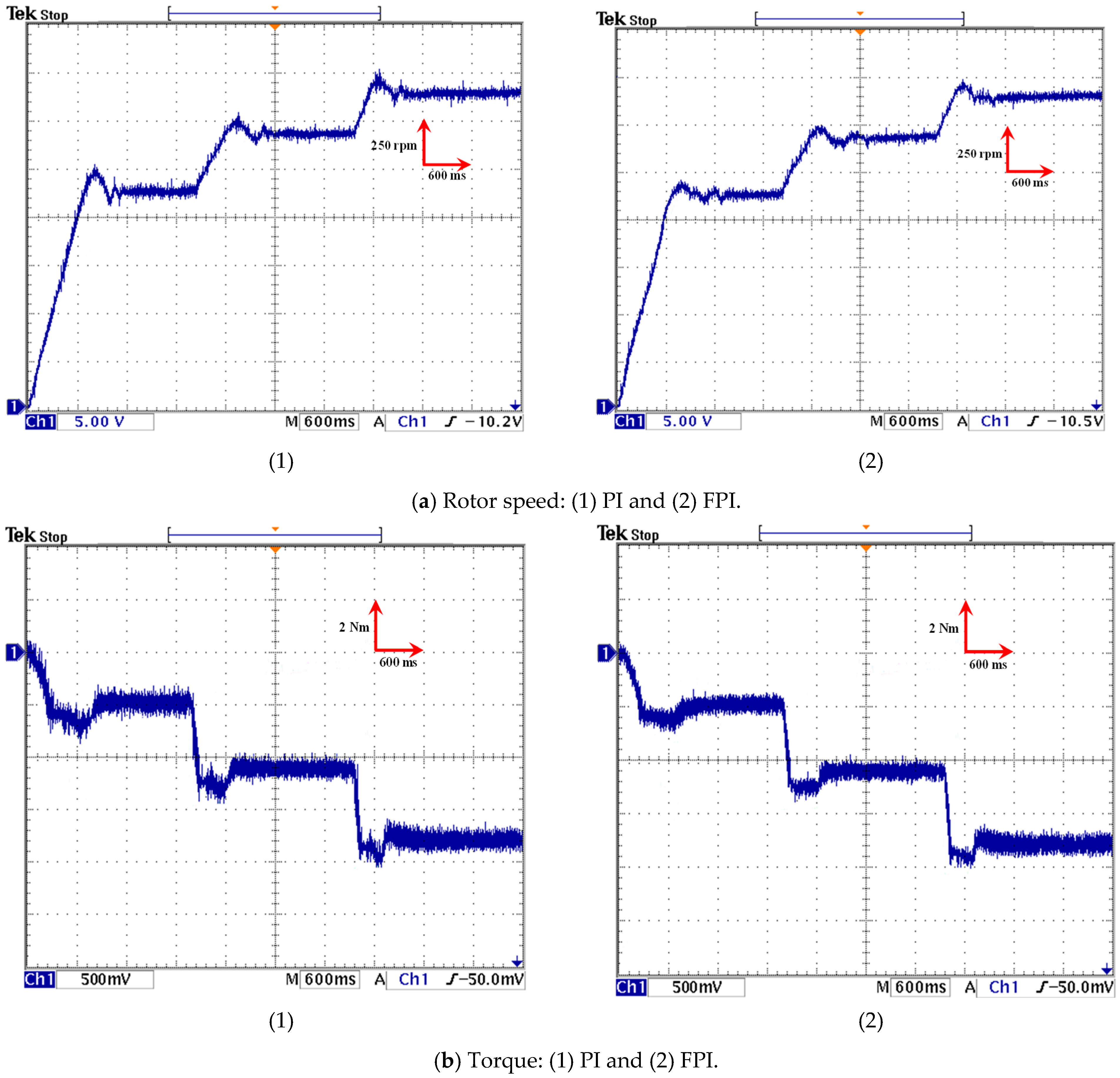
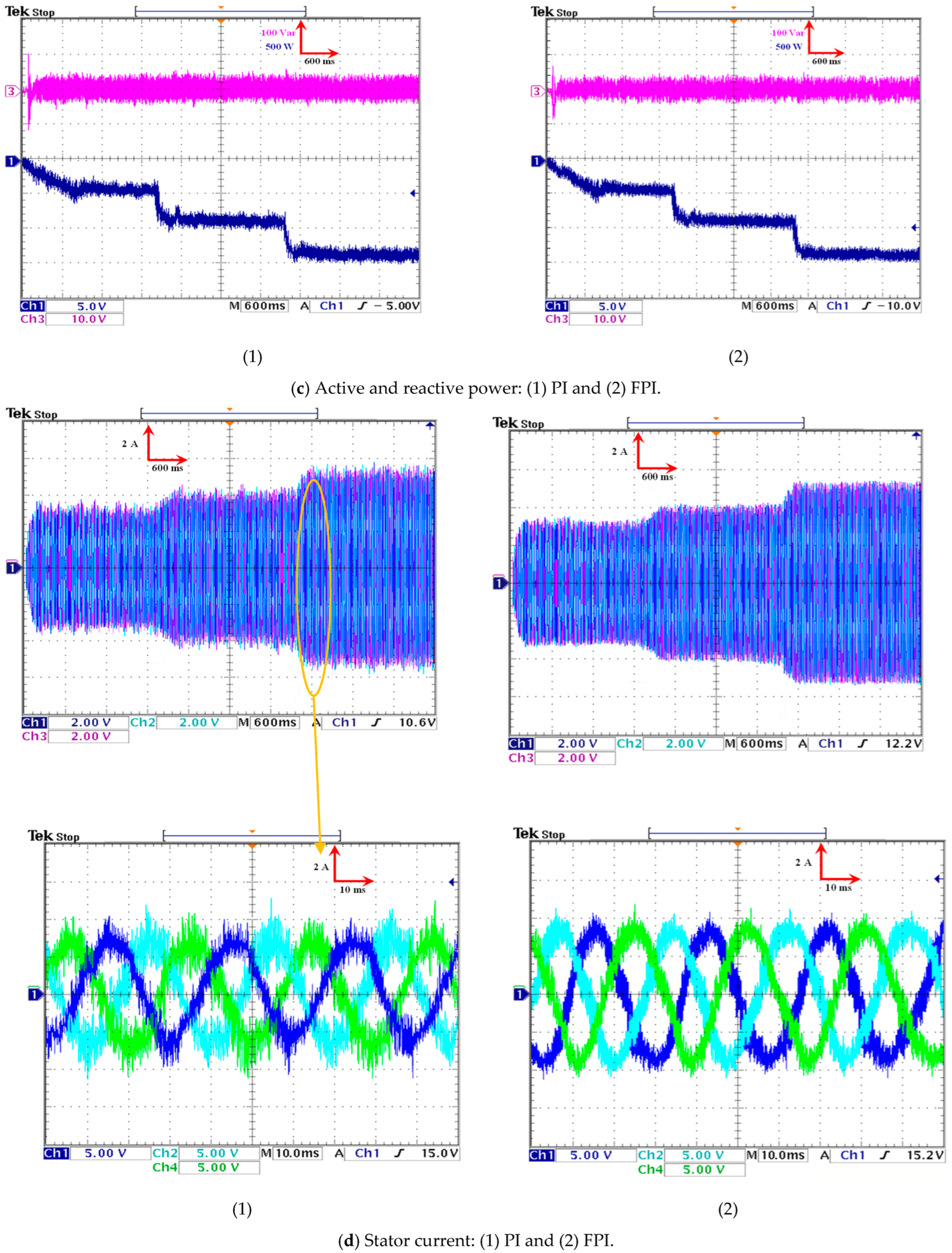
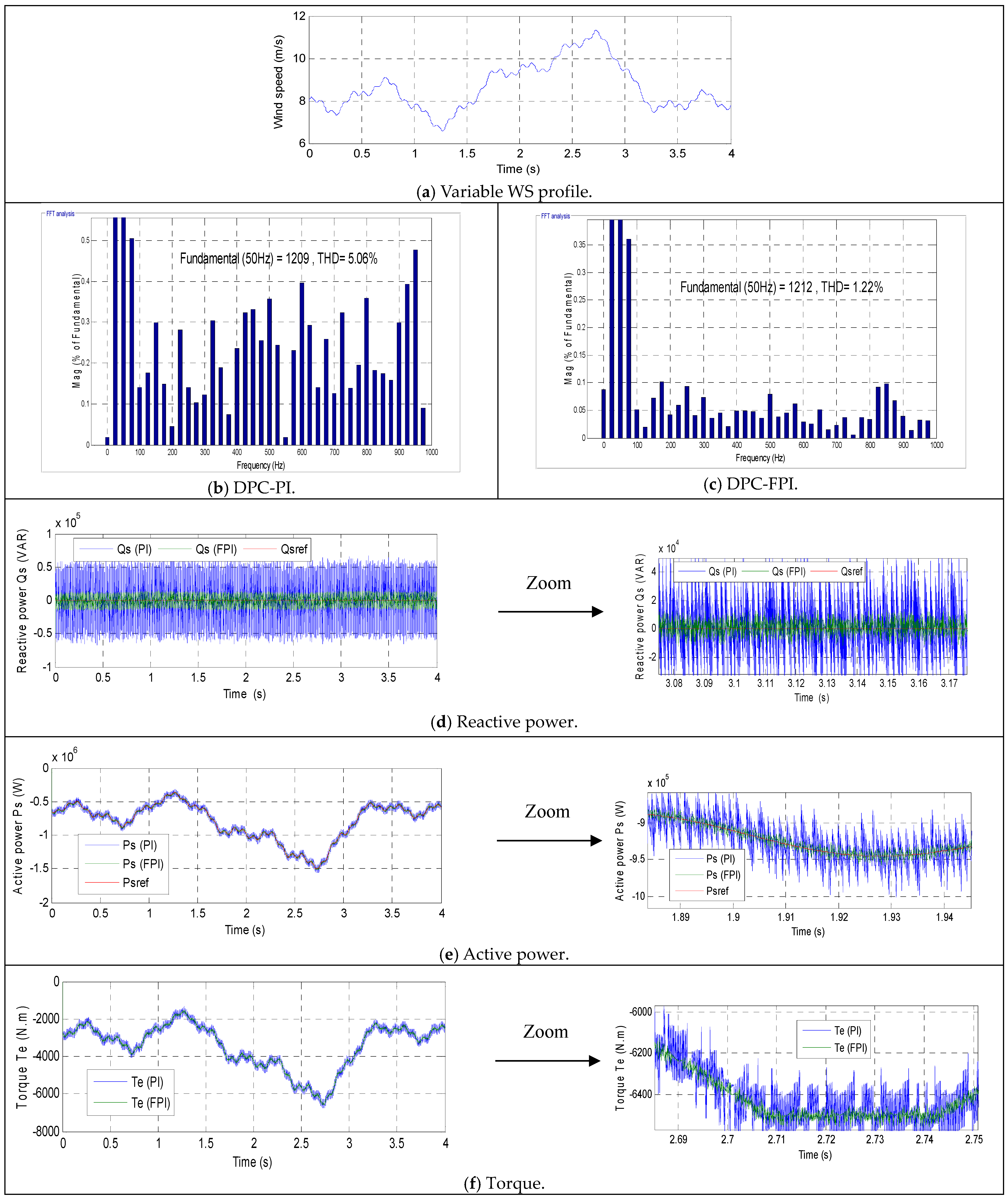
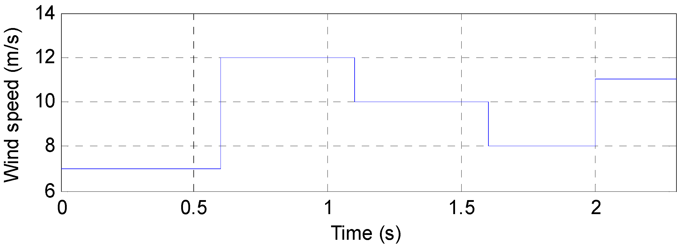
Initially, the strategies delineated in this paper are subjected to empirical scrutiny under standard operating conditions, employing variable WSs. This speed is illustrated in Figure 3a. The numerical results are presented in

Table 5. Reduction rates obtained in test 1.

	Approaches	Qs (VAR)	Ps (W)
SSE	PI	35,050	30,660
	FPI	4200	480
	Ratios (%)	88.01	98.43
Overshoot	PI	14,925	20,910
	FPI	7510	17,830
	Ratios (%)	49.68	14.72
Response time (ms)	PI	0.055	0.80
	FPI	3.20	3.18
	Ratios (%)	−98.28	−74.84
Fluctuations	PI	128,862	100,000
	FPI	25,000	15,000
	Ratios (%)	80.59	85

, while the experimental results are illustrated in Figure 3b–g.

Figure 3b,c illustrate the THD of current for the two algorithms. The THD was estimated to be 1.22% for the FPI regulator and 5.06% for the PI regulator. The values obtained from the analysis indicate that the THD is significantly lower, by 87.74%, in comparison to the PI. The efficacy of the FPI is evidenced by the observed ratio, which indicates its superior performance in enhancing current quality when compared to the PI regulator. Also, Figure 3b,c show that the amplitude value of the fundamental signal (FS) was estimated to be 1209 A when using a PI regulator, while the amplitude value was estimated to be 1212 A when using an FPI regulator. Therefore, the amplitude value is higher when using an FPI regulator, indicating the effectiveness and efficiency of this regulator compared to the classical regulator. The FPI regulator improved the amplitude value of the Fs (50 Hz) by a percentage estimated at 0.24% compared to the PI regulator.

Figure 3d,e illustrate the power variations for the two algorithms under normal operating conditions. These figures demonstrate that the power closely follows the reference values, with a rapid dynamic response. As illustrated in Figure 3e, the active power is contingent upon the variation in the WS, attaining negative values, thereby substantiating the system’s capacity to generate power. However, the Qs remain constant when the WS changes, assuming a value of 0 VAR, as illustrated in Figure 3d. Furthermore, evidence of ripples has been observed across these powers. As illustrated in Table 5, the implementation of the FPI regulator led to a significant minimization in oscillations, with an 80.59% and 85% decrease compared to the PI regulator for Ps and Qs, respectively. In addition, the FPI regulator demonstrated a marked reduction in both SSE and overshoot of Ps, with percentages of 88.01% and 49.68%, respectively, in comparison to the PI regulator. In the case of Qs, the FPI regulator reduced SSE and overshoots by 98.43% and 14.72%, respectively, compared to the PI regulator. However, in terms of response time, the FPI regulator exhibited an unsatisfactory response time in comparison to the PI regulator, as demonstrated in Table 5. As illustrated in Table 5, the PI demonstrated a superior response time, with ratios of 98.28% and 74.84% for Ps and Qs, respectively. In this particular experiment, the response time to the power can be regarded as the negative of the FPI regulator. This negative can be attributed to the gain values. The potential exists for the utilization of alternative or novel algorithms in the future to overcome the aforementioned challenges.

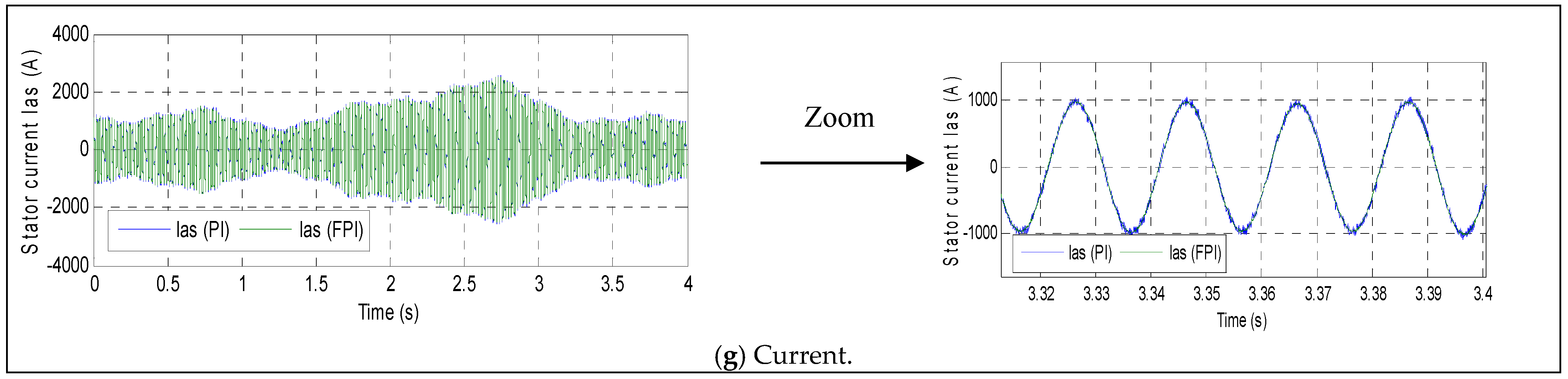
Figure 3f,g illustrate the variations in both torque and current under normal operating conditions. As illustrated in Figure 3f, the torque exhibits a direct correlation with the variation in Ps, attaining negative values under certain conditions. Additionally, ripples are observed in this torque level for both controls. The estimated values for these fluctuations were 400 N·m and 100 N·m for PI and FPI, respectively. Therefore, it can be concluded that the fluctuations are reduced by 75% when using an FPI regulator compared to a PI regulator.

As illustrated in Figure 3g, the current exhibits a sinusoidal variation in accordance with the modulation of Ps, thereby demonstrating a dynamic interplay between these variables. Additionally, the current time interval for both algorithms is 0.02 s. Furthermore, fluctuations in this current level are observed when both algorithms are utilized. The estimated fluctuations are 55.80 A and 23.11 A for PI and FPI, respectively. Therefore, the current fluctuations are reduced by 58.58% in the case of using the FPI regulator, as compared to the PI.

The simulation results in the first test showed an 87.74% reduction in current harmonic distortion, and a significant minimization in current ripple (58.58%) and Ps ripple (85%), demonstrating the powerful controller’s ability to improve PQ and dynamic performance. However, its practical effectiveness still needs to be verified, as operational systems are affected by disturbances, parameter changes, and problems with imperfect devices, such as switching delays and measurement noise. Therefore, further testing is essential to confirm the controller’s robustness and stability under real-world operating conditions. Accordingly, the next test verifies the FPI regulator’s reliability under varying DFIG parameters.

• Case 2: Working under unusual circumstances

In this instance, the efficacy of the FPI regulator is evaluated under atypical conditions by employing the identical WS profile utilized in the initial case. In this particular instance, the generator parameters undergo modification, entailing a multiplication of the resistance values by 2 and a multiplication of the inductance values by 0.5. The results of this study are presented in Figure 4 and Table 6.

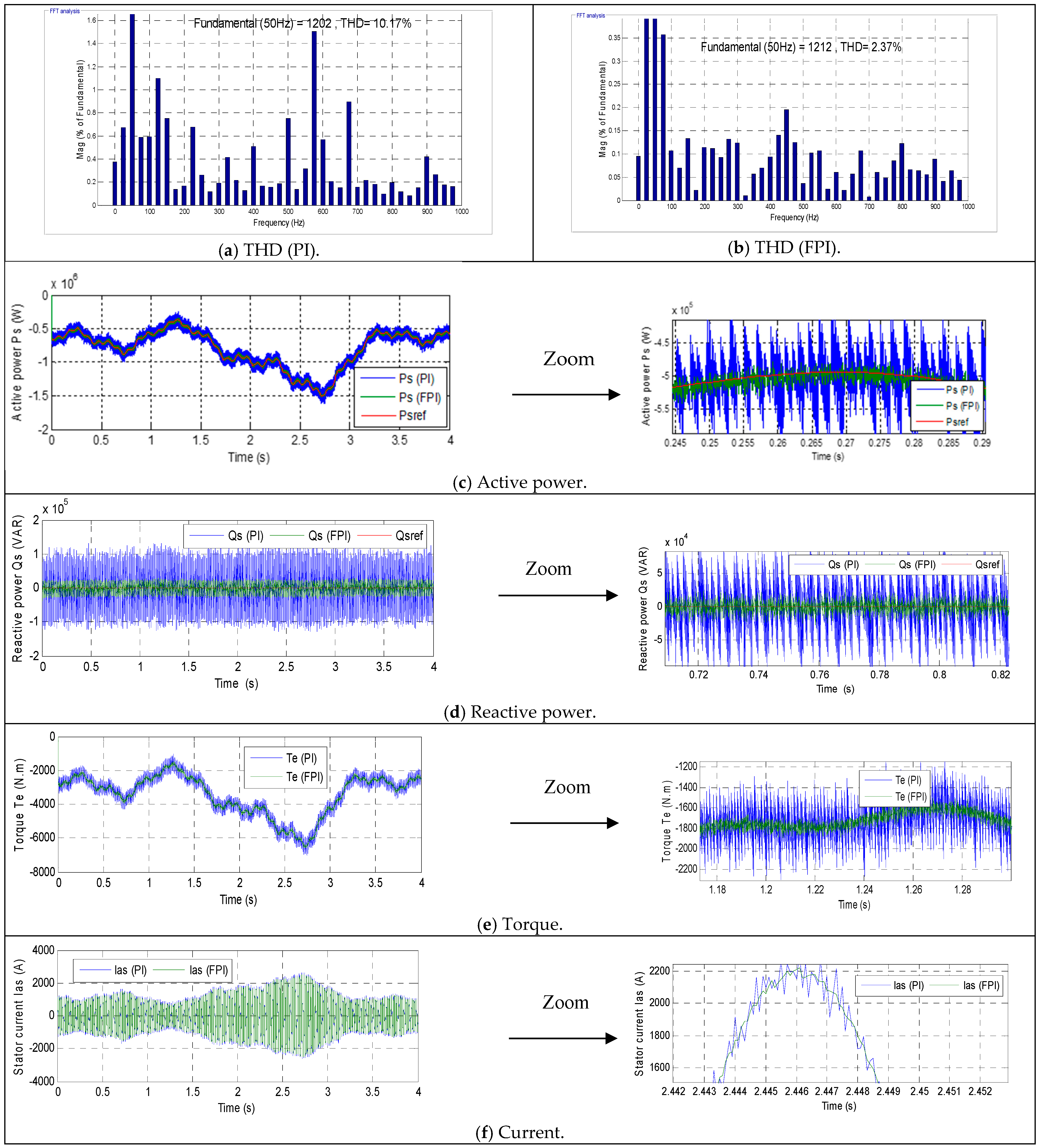
As illustrated in Figure 4a,b, the THD values for the two algorithms are presented under the condition of altering the DFIG parameters. The THD exhibited a substantial increase in this instance, relative to the initial case, attributable to the alterations in parameters. In addition, the THD values in this instance were estimated to be 10.17% and 2.37% for the PI and FPI, respectively. Consequently, the THD in this instance is 76.69% lower than that of the PI regulator. A comparison of the two cases reveals a significant alteration in THD, with a 50.24% change observed in the PI and a 48.52% change in the FPI. These ratios suggest that the THD is less influenced by parameter changes when employing the FPI regulator compared to the PI regulator. Also, Figure 4a,b show that the amplitude of the FS (50 Hz) was 1202 A when using a PI regulator and 1212 A when using an FPI regulator. These values indicate that the FPI regulator provided a better amplitude than the PI by a factor of 0.82%. This observation validates the robustness and effectiveness of the FPI regulator. The findings indicate that the regulator under consideration is a reliable solution for industrial applications.

Figure 4. Second test results.

Figure 4. Second test results.

Figure 4c,d illustrate the alterations in power associated with the two algorithms in case 2. Notwithstanding the alteration in the parameters of the DFIG, the power continues to fluctuate in accordance with the variation in references, exhibiting an augmentation in ripples in comparison to case 1. Furthermore, Figure 4c demonstrates that the active power consistently exhibits negative values, thereby suggesting that the system is indeed generating energy. The Ps value undergoes fluctuations in accordance with variations in WS. Consequently, alterations in DFIG parameters do not impact the variation in Ps for either algorithm. As demonstrated in Figure 4d, the Qs remains at a constant value of zero and is not influenced by variations in WS. As illustrated in Table 6, the FPI demonstrated superior performance in terms of energy characteristics, as evidenced by its significantly improved numerical values for oscillations, SSE, and overshoot when compared to the PI regulator.

Table 6. Reduction rates obtained in test 2.

	Approaches	Qs (VAR)	Ps (W)
SSE	PI	44,480	15,900
	FPI	11,395	7100
	Ratios (%)	74.38	55.34
Overshoot	PI	29,150	6290
	FPI	19,944	5600
	Ratios (%)	31.58	10.96
Response time (ms)	PI	0.056	0.53
	FPI	1.82	1.77
	Ratios (%)	−96.92	−70.05
Fluctuations	PI	259,130	200,000
	FPI	48,200	30,000
	Ratios (%)	81.39	85

Table 6. Reduction rates obtained in test 2.

	Approaches	Qs (VAR)	Ps (W)
SSE	PI	44,480	15,900
	FPI	11,395	7100
	Ratios (%)	74.38	55.34
Overshoot	PI	29,150	6290
	FPI	19,944	5600
	Ratios (%)	31.58	10.96
Response time (ms)	PI	0.056	0.53
	FPI	1.82	1.77
	Ratios (%)	−96.92	−70.05
Fluctuations	PI	259,130	200,000
	FPI	48,200	30,000
	Ratios (%)	81.39	85

In the Ps state, the FPI regulator demonstrated a significant minimization in ripple, overshoot, and SSE, with percentages of 85%, 10.96%, and 55.34%, respectively, in comparison to the PI. In Qs state, the FPI regulator demonstrated a marked improvement in various performance metrics when compared to the PI regulator. These enhancements included an 81.39% reduction in ripple, a 31.58% reduction in overshoot, and a 74.38% reduction in SSE. The efficacy of the FPI regulator in improving PQ is demonstrated by these ratios, rendering it a promising solution. However, despite this performance, the FPI regulator delivered unsatisfactory power response times compared to the PI, as shown in Table 6. The findings of the present study demonstrate that the PI regulator diminished response times by 96.92% and 70.05% for both Qs and Ps, respectively, in comparison with the FPI regulator. Consequently, the response time is also a drawback of the FPI in this case. It is possible to surmount this drawback by employing alternative strategies. Comparing the results for Case 2 with Case 1, the ripple, SSE, and overshoot values increased significantly, especially when the PI regulator was used. For Ps, the oscillation, SSE, and overshoot values increased by 50%, 93.23%, and −68.59%, respectively, when the FPI regulator was used. For PI, the oscillation, SSE, and overshoot values for Ps increased by 50%, −48.14%, and −69.91%, respectively. In the case of the Qs, the ripple, overshoot, and SSE values increased in Case 2 compared to Case 1 by 48.13%, 62.34%, and 63.14%, respectively, when the FPI regulator was used. In the case of PI, the oscillation, overshoot, and SSE values increased in Case 2 compared to Case 1 by 50.27%, 48.79%, and 26.90%, respectively.

Figure 4e illustrates the torque change over time when both algorithms are employed. From this figure, it is evident that modifying the DFIG parameters does not impact the torque change, as the shape remains congruent with the change in Ps. Additionally, it is discernible that the torque values persist in being negative despite the alteration in the machine parameters, which is consistent with the observation made in Case 1. In Case 2, it was observed that the torque fluctuations increased significantly when both algorithms were used. The torque ripples in Case 2 were estimated at 800 N·m and 158.20 N·m for the PI and FPI, respectively. The findings indicate that the torque fluctuations are reduced by 80.22% with the FPI regulator in comparison with the PI.

In comparison to Case 1, torque ripples exhibited an increase of 50% and 36.78%, respectively, for the PI and FPI. Therefore, the FPI regulator demonstrated a significantly reduced torque ripple effect in comparison to the PI regulator. This outcome serves to underscore the enhanced robustness and efficacy of the FPI regulator.

As illustrated in Figure 4f, the current variation for the two algorithms in Case 2 is represented. This current maintains a sinusoidal pattern despite the alteration in the generator parameters, where a heightened ripple is observed in comparison to Case 1. This increase in ripple is more pronounced when using a PI compared to an FPI. It is also noteworthy that the current fluctuations for both algorithms persistently change according to the variation in Ps, a finding that was also observed in test 1. In Case 2, the current ripples attained a value of 196.80 A when the PI regulator was employed and a value of 41 A when the FPI regulator was utilized. These values indicate that ripples are significantly lower when using the FPI regulator. This reduction is estimated at 79.16% compared to the PI. A comparison of the two cases reveals a substantial increase in the ripple current in Case 2, attributable to the modification of DFIG parameters. The estimated change in ripple was 71.64% for the PI regulator and 43.63% for the FPI regulator. These ratios indicate that the FPI regulator exhibited a significantly lower ripple effect than the PI regulator, thereby highlighting its robustness in enhancing current quality despite varying DFIG parameters. The findings indicate that the FPI is a viable solution for a range of applications, including electric vehicles and photovoltaic systems.

• Case 3: Step WS profile

In this case, the new algorithm is tested using a different WS profile than the one used in the first test. This profile is shown in Figure 5. In this test, the DFIG or turbine parameters remain unchanged. This test aims to explore the behavior of the new algorithm under sudden and rapid changes in WS, comparing its performance to the PI approach. The graphical results of this test are shown in Figure 6, while the numerical results are shown in Table 7.

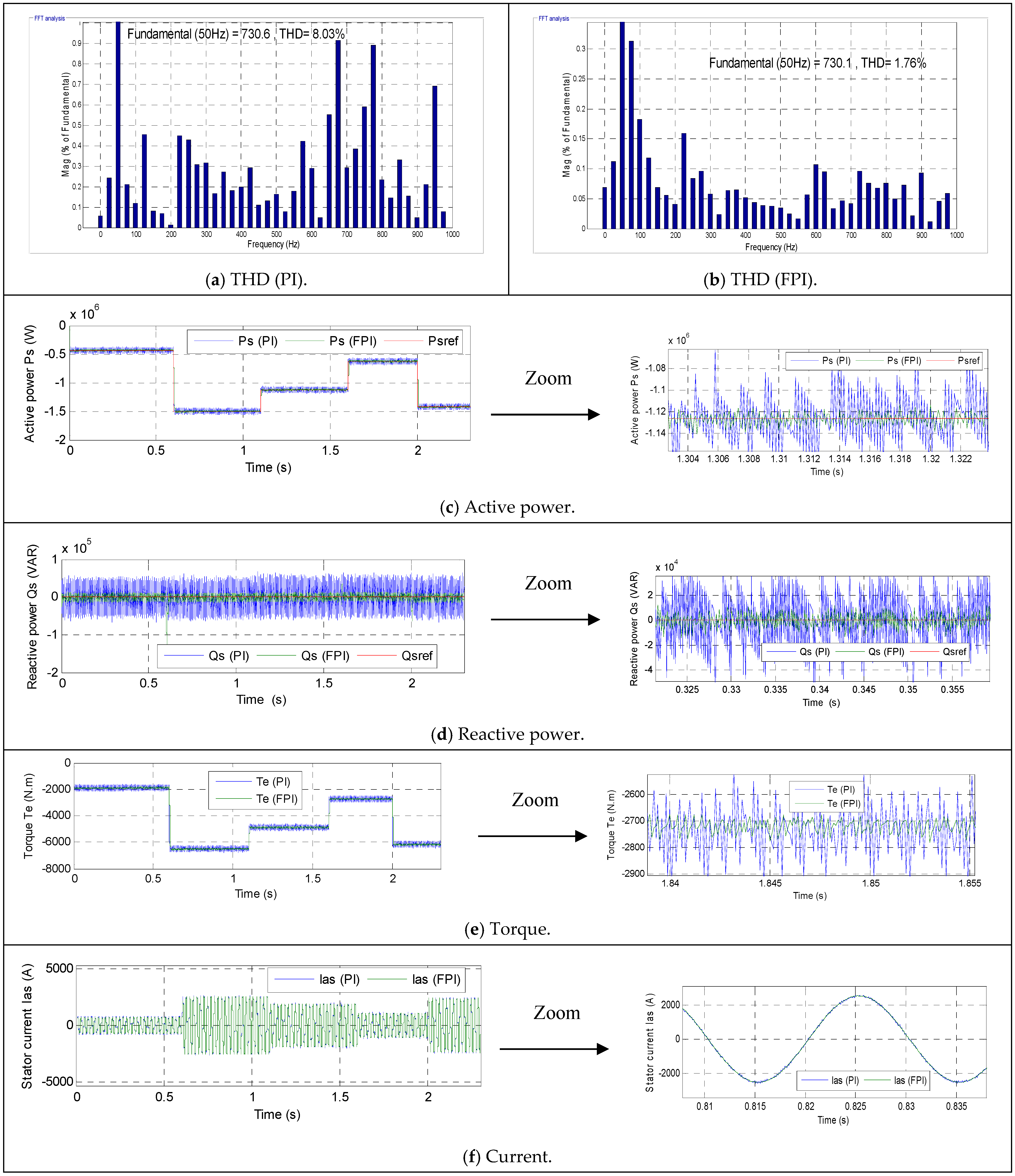
Figure 6a,b represent the THD values of stator current and the amplitude of FS (50 Hz) of current when using both controls. From these figures, it is noted that the THD values were estimated to be 8.03% and 1.76% for PI and FPI, respectively. Based on these values, the FPI regulator significantly reduced the THD value compared to the PI regulator. This reduction was estimated at 78.08%. Furthermore, it was noted that the regulators provided almost the same value for the FS amplitude. These results indicate the effectiveness of the FPI regulator in improving current quality, as shown in the graphs.

Figure 6c represents the change in Ps under a sudden and rapid change in WS. From this figure, the Ps of the two controls varies with the change in WS, taking on negative values, similar to the results of the previous tests. Also, oscillations are observed in this power level when using both controls. Figure 6c shows that the power has a fast dynamic response when using both controllers, with the PI controller having an advantage over the FPI controller. According to Table 7, the response time of the Ps is 68.44% better with the PI controller than with the FPI controller. However, it is noted from Table 7 that the FPI regulator gave significantly better values for ripple, overshoot, and SSE than the PI regulator. Therefore, the FPI regulator reduced the fluctuation, overshoot, and SSE values of the Ps by 80%, 38.18%, and 87.21%, respectively, compared to the PI regulator.

Figure 6. Third test results.

Figure 6. Third test results.

Figure 6d represents the change in Qs under a sudden and rapid change in WS. Despite the rapid and sudden changes in WS, this power remains unchanged, remaining constant under both controls. This value is estimated at 0 VAR. Furthermore, it is noted that the Qs has a rapid dynamic response and the presence of ripples. These ripples, according to Table 7, are significantly lower when using the FPI compared to the PI controller. According to Table 7, the FPI regulator reduced the Ps ripple by 79.83% compared to the PI. Furthermore, Table 7 shows that the FPI provided better SSE and overshoot values than the PI regulator, with values of 77.40% and 90.91%, respectively. However, the FPI regulator provided unsatisfactory Qs response time compared to the PI regulator, as shown in Table 7. The Qs response time is better with the PI regulator, with a value of 97.22%.

Figure 6e represents the torque variation under a sudden and rapid change in WS. Despite the rapid change in WS, the torque variation remains in the form of a change in Ps, which is the same as in the tests above. The torque remains negative, indicating that the system is transmitting power to the grid. In this test, the torque ripples were estimated at 400 N·m and 80 N·m for the FPI and PI regulators, respectively. These values indicate that torque ripples are significantly lower when using the FPI controller at a ratio of 80% compared to the PI controller.

Figure 6f represents the current variation over time for the two designed controls. Despite the rapid and sudden change in WS, the current remains sinusoidal, with a period of 0.02 s for both algorithms. Also, it is noted that the current value varies with the change in WS, similar to the observations in the tests above. The current ripples in this test were estimated at 60 A and 23.20 A for the PI and FPI, respectively. Therefore, the regulator minimized the current ripple by 61.33% compared to the PI regulator.

Table 7. Minimization rates obtained in the third test.

	Algorithms	Ps (W)	Qs (VAR)
SSE	PI	26,600	28,794
	FPI	3400	6500
	Ratios (%)	87.21	77.40
Overshoot	PI	23,700	14,925
	FPI	14,650	1356.20
	Ratios (%)	38.18	90.91
Response time (ms)	PI	0.65	0.055
	FPI	2.06	1.98
	Ratios (%)	−68.44	−97.22
Fluctuations	PI	100,000	124,000
	FPI	20,000	25,000
	Ratios (%)	80	79.83

Table 7. Minimization rates obtained in the third test.

	Algorithms	Ps (W)	Qs (VAR)
SSE	PI	26,600	28,794
	FPI	3400	6500
	Ratios (%)	87.21	77.40
Overshoot	PI	23,700	14,925
	FPI	14,650	1356.20
	Ratios (%)	38.18	90.91
Response time (ms)	PI	0.65	0.055
	FPI	2.06	1.98
	Ratios (%)	−68.44	−97.22
Fluctuations	PI	100,000	124,000
	FPI	20,000	25,000
	Ratios (%)	80	79.83

• Case 4: Operation at cut-in and cut-out speeds

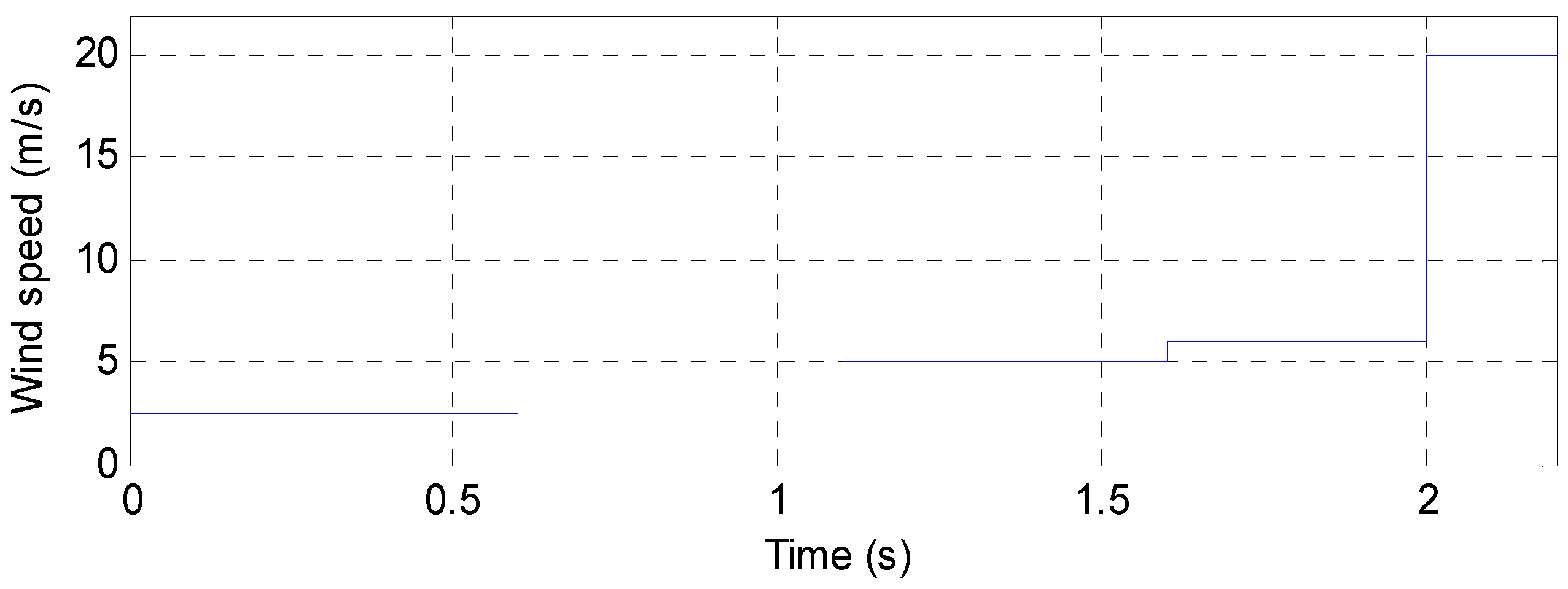
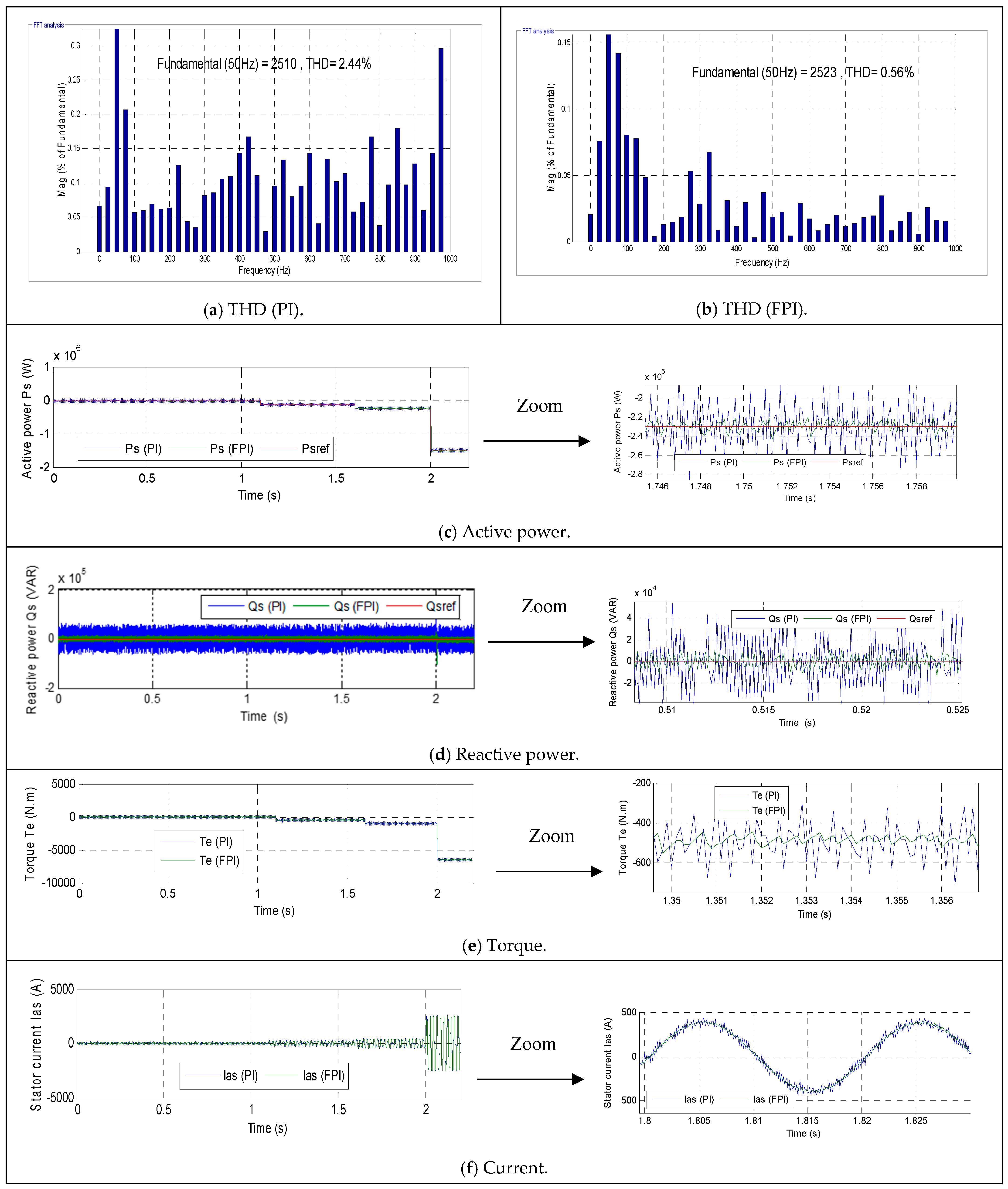
This test investigates the efficacy and effectiveness of the FPI regulator at cut-in and cut-out WSs, comparing its performance to that of a PI controller. WSs were used in this test as follows: 2.5 m/s, 3 m/s, 5 m/s, 6 m/s, and 20 m/s. The WS variation diagram used is shown in Figure 7. The graphical results of this test are shown in Figure 8, while the numerical results are listed in Table 8 and Table 9.

Figure 8a,b show the THD values for the stator current and the FS (50 Hz) amplitude for the current at cut-in and cut-out speeds. Furthermore, the amplitude and THD values are listed in Table 8. This table demonstrates that the THD value at cut-in speeds is significantly higher when using both controllers, with the FPI controller being preferable to the PI controller. However, the amplitude of the FS (50 Hz) is low at cut-in speeds and increases with WS, becoming greater at cut-out speeds. Therefore, WS significantly affects the THD value and its amplitude. According to Table 8, the THD value is significantly lower compared to the PI controller, by 79.16%, 79.14%, 80.24%, 77.43%, and 77.04% for 0.1, 0.7, 1.4, 1.8, and 2.1 s, respectively. Also, Table 8 shows that the FPI controller provided a greater duration at WSs of 2.5 m/s and 5 m/s, by 1.52% and 1%, respectively, compared to the PI. At a WS of 3 m/s, both regulators provided the same amplitude. However, at a WS of 6 m/s, the FPI produced unsatisfactory amplitude compared to the PI. Furthermore, it was observed that the FPI controller, at a WS of 20 m/s, provided a 0.51-fold greater amplitude compared to the PI. These results indicate the superior effectiveness of the FPI compared to the PI controller in improving current quality at both very low and high WSs.

Figure 7. Cut-in and cut-out WS profile.

Figure 7. Cut-in and cut-out WS profile.

Figure 8c,d represent the change in power over time for the two techniques. Figure 8c shows that the Ps at low WSs (2.5 and 3 m/s) are zero when using both controls with ripples. At a WS of 5 m/s, the Ps of both controls become negative, indicating that the system is generating power. At a WS of 6 m/s, the power output is greater compared to 5 m/s. Figure 8c shows that at a strong WS (20 m/s), the system under consideration generates a higher Ps output with better quality compared to lower WSs.

In the case of cut-in speed, the FPI controller reduced the SSE and overshoot values of Qs by 60.24% and 82.18%, respectively, compared to the PI (see Table 9). In the case of cut-out speed, the FPI controller reduced the SSE and overshoot values of Qs by 83.71% and 52.44%, respectively, compared to the PI.

The FPI reduced the SSE of Ps by 84.29% and 53.22% for both cut-in and cut-out speeds, respectively, compared to the PI controller. While the overshoot of Ps is significantly lower, as shown in Table 9, when using the FPI regulator, by 81.78% and 11.35% for cut-in and cut-out speeds, respectively, compared to the PI approach, these percentages indicate the effectiveness and efficiency of the FPI-based command in improving PQ at cut-in and cut-out speeds. However, the FPI controller provided unsatisfactory power delivery times at cut-in and cut-out speeds compared to the PI controller. Therefore, power delivery times are also a drawback of the FPI controller at both low and high WSs. This drawback can be mitigated and overcome in the future.

Figure 8e represents the torque variation under cut-in and cut-out speeds. This figure shows that the torque value at speeds of 2.5 m/s and 3 m/s is zero when both regulators are used and large ripples are present. Figure 8e also shows that the turbine generates torque at WSs up to 5 m/s. It is observed that increasing WS significantly increases the torque value, with the highest torque values occurring at high WSs. Figure 8e shows the highest torque value at a WS of 20 m/s. The torque values at the cut-in speed were 400 N·m and 43.85 N·m for PI and FPI, respectively. In the case of cut-out speed, the torque values were estimated at 435 N·m and 67 N·m for PI and FPI, respectively. These values indicate that torque quality is better when using FPI and that torque ripple is greater in the cut-out case compared to the cut-in case. These results require further investigation through future work and experimentation.

Figure 8. Fourth test results.

Figure 8. Fourth test results.

Figure 8f illustrates the change in current at both cut-in and cut-out speeds. This figure shows that at low WSs (2.5 m/s and 3 m/s), the current is negligible with significant ripples. Furthermore, current is generated at a WS of 5 m/s, where the current value increases until it reaches its maximum value at the cut-out speed. Figure 8f shows that the current signal period for the two algorithms is 0.02 s at both low and high WSs. It is also observed that the current quality is significantly better at high WSs compared to low WSs. At low WSs, the current oscillations were estimated at 110 A and 13.5 A for the PI and FPI regulators, respectively. These values indicate that the current ripple is significantly lower with the FPI controller (88%) compared to the PI regulator. Furthermore, the current ripple at high WSs (20 m/s) was 44.35 A with the PI and 14 A with the FPI. Therefore, the FPI controller significantly reduced current ripple at high WSs by approximately 68% compared to the PI regulator. These results indicate that current quality improves considerably with high WSs, and the FPI regulator is more efficient at both low and high WSs compared to the PI regulator.

Table 8. Reduction rates for THD value and amplitude of fundamental signal obtained in the fourth test.

Algorithms		0.1 s	0.7 s	1.4 s	1.8 s	2.1 s
THD (%)	PI	100.40	98.16	32.09	15.29	2.44
	FPI	20.92	20.47	6.34	3.45	0.56
	Ratios (%)	79.16	79.14	80.24	77.43	77.04
Fundamental signal (50 Hz) Amplitude (A)	PI	61.37	61.69	196.20	390.90	2510
	FPI	62.32	61.69	198.20	390.40	2523
	Ratios (%)	1.52	0	1	−0.12	0.51

Table 8. Reduction rates for THD value and amplitude of fundamental signal obtained in the fourth test.

Algorithms		0.1 s	0.7 s	1.4 s	1.8 s	2.1 s
THD (%)	PI	100.40	98.16	32.09	15.29	2.44
	FPI	20.92	20.47	6.34	3.45	0.56
	Ratios (%)	79.16	79.14	80.24	77.43	77.04
Fundamental signal (50 Hz) Amplitude (A)	PI	61.37	61.69	196.20	390.90	2510
	FPI	62.32	61.69	198.20	390.40	2523
	Ratios (%)	1.52	0	1	−0.12	0.51

Table 9. Minimization rates obtained in the fourth test.

Approaches		Cut-In Speed		Cut-Out Speed
		Ps (W)	Qs (VAR)	Ps (W)	Qs (VAR)
SSE	PI	29,735	26,664	12,400	37,858
	FPI	4700	10,600	5800	6167
	Ratios (%)	84.29	60.24	53.22	83.71
Overshoot	PI	54,255	14,920	18,500	25,812
	FPI	9880	2658	16,400	12,275
	Ratios (%)	81.78	82.18	11.35	52.44
Response time (ms)	PI	0.013	0.055	2.10	0.1
	FPI	0.056	0.26	7.8	0.1
	Ratios (%)	−76.78	−78.84	−73.07	0
Fluctuations	PI	20,000	120,000	103,800	111,800
	FPI	5000	20,000	20,000	22,514
	Ratios (%)	75	83.33	80.73	79.86

Table 9. Minimization rates obtained in the fourth test.

Approaches		Cut-In Speed		Cut-Out Speed
		Ps (W)	Qs (VAR)	Ps (W)	Qs (VAR)
SSE	PI	29,735	26,664	12,400	37,858
	FPI	4700	10,600	5800	6167
	Ratios (%)	84.29	60.24	53.22	83.71
Overshoot	PI	54,255	14,920	18,500	25,812
	FPI	9880	2658	16,400	12,275
	Ratios (%)	81.78	82.18	11.35	52.44
Response time (ms)	PI	0.013	0.055	2.10	0.1
	FPI	0.056	0.26	7.8	0.1
	Ratios (%)	−76.78	−78.84	−73.07	0
Fluctuations	PI	20,000	120,000	103,800	111,800
	FPI	5000	20,000	20,000	22,514
	Ratios (%)	75	83.33	80.73	79.86

The data in Table 10 provide a statistical comparison between the conventional PI and the FPI regulator in terms of stator Ps ripples and THD. The improvement ratios are listed in Table 11 for the two controls. Under the PI regulator, the Ps ripples fluctuate between 100,000 and 200,000 W, with an average of 125,950 W and a standard deviation of 42,780.92 W. This indicates a highly oscillating power pattern, showing that the PI regulator is struggling to maintain a stable power output, resulting in significant variations and instability in the Ps flow. Under the FPI controller, Ps ripples are significantly reduced, ranging only between 15,000 and 30,000 W, with an average of 21,250 W and a much smaller standard deviation of 5448.62 W. This reflects a substantial reduction in Ps oscillation (an improvement of approximately 83%), indicating that the FPI controller provides superior damping and smoother power delivery. The decrease in both mean deviation and standard deviation shows that the FPI regulator stabilizes electromagnetic energy more effectively, reducing oscillations that can lead to mechanical stress, voltage fluctuations, and reduced power conversion efficiency.

The PI regulator produces THD values ranging from 2.44% to 10.17%, with a mean of 6.43% and a standard deviation of 2.93%. This variability indicates inconsistent current waveform quality, which is often associated with nonlinear responses and poor modulation accuracy. In contrast, the FPI regulator achieves THD values ranging from 0.56% to 2.37%, with an average of 1.48% and a low standard deviation of 0.67%. This demonstrates stability and low harmonic content, indicating a near-sine waveform and improved converter modulation accuracy. The reduction in THD by approximately 77% (see Table 11) confirms the FPI regulator’s ability to reduce high-frequency harmonic components, resulting in better PQ, lower losses, and smoother torque in the DFIG system. Therefore, the low mean and standard deviation values for both Ps ripples and THD under FPI control indicate improved performance, as well as enhanced consistency and robustness. Also, the results suggest that the FPI regulator provides superior compensation for dynamic errors, leading to reduced power fluctuations, purer current spectra, and increased system efficiency.

From a system perspective, this improvement translates directly into smoother torque, reduced mechanical vibrations, reduced transformer stress, and extended system life.

Table 10. Statistical study of Ps ripples and THD values of the suggested methods.

Approaches		Ps Ripples	THD	Minimum Value		Maximum Value		Average Value		Standard Deviation
				Ps Ripples	THD	Ps Ripples	THD	Ps Ripples	THD	Ps Ripples	THD
PI	Test 1	100,000 W	5.06%	100,000 W	2.44%	200,000 W	10.17%	125,950 W	6.43%	42,780.92 W	2.93%
	Test 2	200,000 W	10.17%
	Test 3	100,000 W	8.03%
	Test 4	103,800 W	2.44%
FPI	Test 1	15,000 W	1.22%	15,000 W	0.56%	30,000 W	2.37%	21,250 W	1.48%	5448.62 W	0.67%
	Test 2	30,000 W	2.37%
	Test 3	20,000 W	1.76%
	Test 4	20,000 W	0.56%

Table 10. Statistical study of Ps ripples and THD values of the suggested methods.

Approaches		Ps Ripples	THD	Minimum Value		Maximum Value		Average Value		Standard Deviation
				Ps Ripples	THD	Ps Ripples	THD	Ps Ripples	THD	Ps Ripples	THD
PI	Test 1	100,000 W	5.06%	100,000 W	2.44%	200,000 W	10.17%	125,950 W	6.43%	42,780.92 W	2.93%
	Test 2	200,000 W	10.17%
	Test 3	100,000 W	8.03%
	Test 4	103,800 W	2.44%
FPI	Test 1	15,000 W	1.22%	15,000 W	0.56%	30,000 W	2.37%	21,250 W	1.48%	5448.62 W	0.67%
	Test 2	30,000 W	2.37%
	Test 3	20,000 W	1.76%
	Test 4	20,000 W	0.56%

Table 11. Improvement rates for statistical results.

Parameters	Controllers		Improvement (%)	Interpretation
	PI	FPI
Average THD	6.43%	1.48%	77%	Better waveform quality
Average Ps ripple	125,950 W	21,250 W	83%	Strong power stabilization
Std. deviation (THD)	2.93%	0.67%	77%	Stable harmonic behavior
Std. Deviation (Ps ripples)	42,780.92 W	5448.62 W	87%	More consistent performance

Table 11. Improvement rates for statistical results.

Parameters	Controllers		Improvement (%)	Interpretation
	PI	FPI
Average THD	6.43%	1.48%	77%	Better waveform quality
Average Ps ripple	125,950 W	21,250 W	83%	Strong power stabilization
Std. deviation (THD)	2.93%	0.67%	77%	Stable harmonic behavior
Std. Deviation (Ps ripples)	42,780.92 W	5448.62 W	87%	More consistent performance

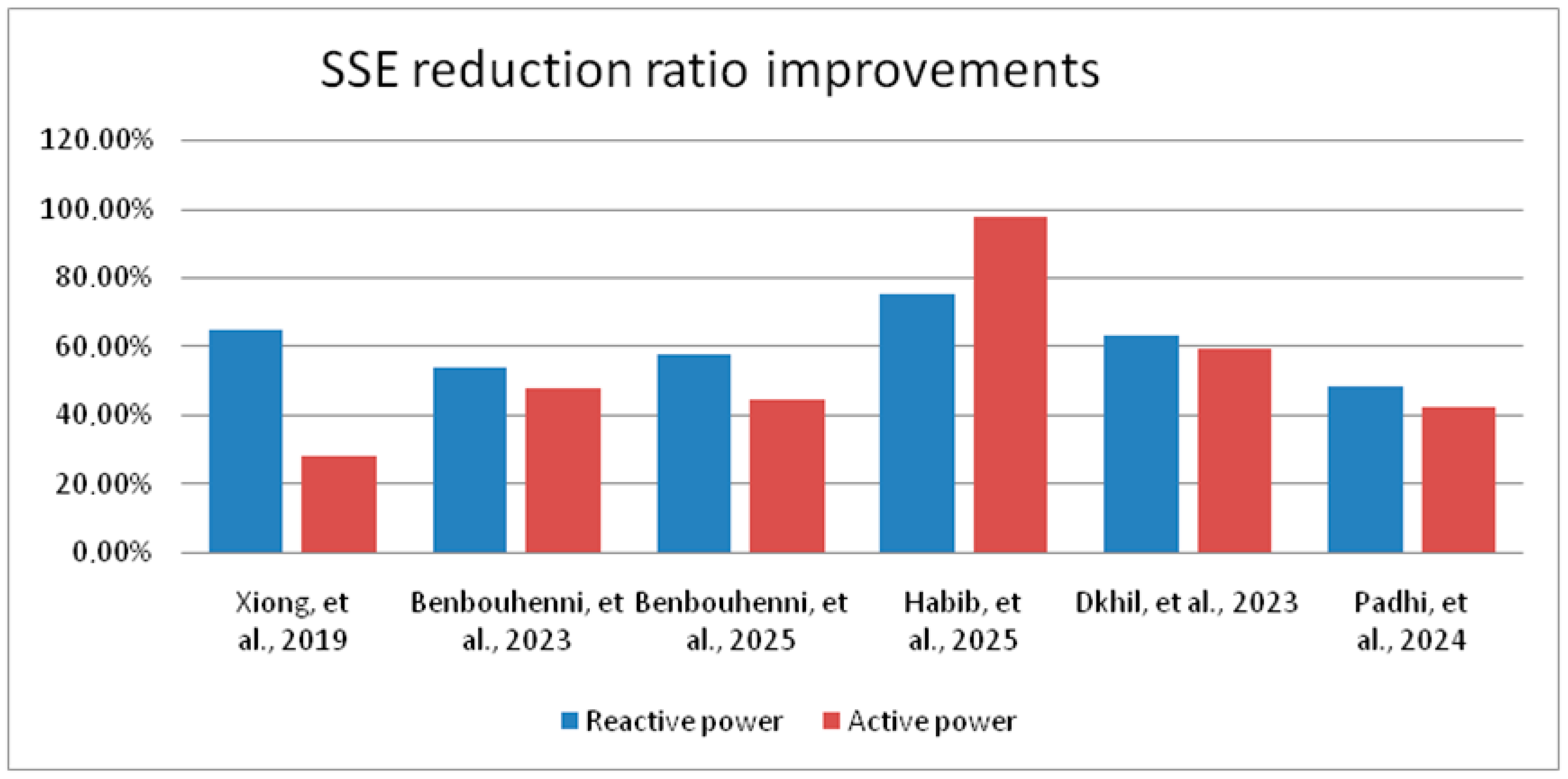
As illustrated in Table 12, an evaluation of the operational performance of the FPI regulator is conducted by comparing it to several research papers in terms of the SSE reduction ratios for power. The results of the first case were used for this comparison. A close examination of the results enumerated in Table 12 reveals that the SSE minimization ratios are considerably higher in the case of the FPI regulator compared to the ratios obtained from algorithms documented in the extant literature. The performance of the FPI was evaluated by calculating the SSE improvement ratios compared to several methods. As illustrated in Table 12, the estimated SSE improvement ratios for Ps were 27.69%, 47.84%, 44.52%, 97.56%, 59.18%, and 41.98%/43.35%, respectively, for [50,51,52,53,54,55]. Consequently, the highest observed improvement ratio was estimated to be 97.56% compared to [53], while the lowest improvement ratio was estimated to be 27.69% compared to [50]. As illustrated in Figure 9, the obtained improvement ratios are presented graphically.

In the context of Qs, the FPI demonstrated a significant enhancement in the SSE value, with improvements ranging from 64.39% to 74.91%, as compared to the findings in [50,51,52,53,54,55], respectively. The ratios demonstrate the capacity, efficacy, and superior performance of the FPI system in comparison to numerous extant algorithms in the existing literature. This observation renders the FPI system a promising contender for future applications. The most significant enhancement ratio was compared to the work [53], estimated at 74.91%. The lowest recorded improvement ratio for the SSE of Qs was estimated at 47.40%, which was compared to the work [55].

Table 12. Comparison table with other businesses in terms of SSE value reduction percentage.

References	SSE Ratios (%)		Improvements
	Qs (VAR)	Ps (W)	Ps (W)	Qs (VAR)
[50]	35.48	62	27.69%	64.39%
[51]	46.16	44.72	47.84%	53.68%
[52]	42.14	47.57	44.52%	57.71%
[53]	25	2.09	97.56%	74.91%
[54]	36.93	35	59.18%	62.94%
[55]	51.85	49.75	41.98%	47.97%
	52.42	48.57	43.35%	47.40%
Suggested algorithm	99.66	85.75	-

Table 12. Comparison table with other businesses in terms of SSE value reduction percentage.

References	SSE Ratios (%)		Improvements
	Qs (VAR)	Ps (W)	Ps (W)	Qs (VAR)
[50]	35.48	62	27.69%	64.39%
[51]	46.16	44.72	47.84%	53.68%
[52]	42.14	47.57	44.52%	57.71%
[53]	25	2.09	97.56%	74.91%
[54]	36.93	35	59.18%	62.94%
[55]	51.85	49.75	41.98%	47.97%
	52.42	48.57	43.35%	47.40%
Suggested algorithm	99.66	85.75	-

5. Experimental Results

As demonstrated in Figure 10, the experimental work conducted in this study elucidates the implementation of the new algorithm and its effectiveness in enhancing the PQ of DFIG. This figure encompasses the majority of the tangible instruments utilized to implement the novel algorithm, including a digital oscilloscope, an RSC control, a speed step controller, and others. The objective of this experimental study is to ascertain the validity and efficacy of the FPI regulator in comparison to the PI regulator, with a focus on enhancing the performance of the PQ and command system characteristics.

The RSC is subject to experimental control through the utilization of a DPC-FPI. In this experimental study, a 3 kW generator with the parameters listed in Table 13 is employed. In this experimental work, the generator is driven by a 3.5 kW synchronous motor. The synchronous motor is operated at varying speeds to simulate step-wise WSs.

The dSPACE 1104 board serves the purpose of establishing a connection between the computer and the experimental apparatus. The dSPACE 1104 board is also employed to create the pulses necessary to operate the machine’s inverter. In this experiment, a two-level inverter was utilized to streamline the process and reduce expenses.

Table 13. Generator parameters in experimental work.

Parameter	Symbol	Value	Unit
Rated power	$Ps$	3000	W
Stator inductance	$Ls$	263	mH
Stator voltage (line-to-line)	$Vs$	326	V
Power factor	$Cos\left(\varphi \right)$	0.86	–
Number of pole pairs	$p$	2	–
Rated speed	–	1450	rpm
Estimated stator current	$Is$	6.18	A
Stator resistance	$Rs$	1.72	Ω
Mutual inductance	$Lm$	185	mH
Rotor resistance	$Rr$	1.95	Ω
Estimated stator current	$Is$	6.18	A
Rotor inductance	$Lr$	270	mH
Stator frequency	$fs$	50	Hz

Table 13. Generator parameters in experimental work.

Parameter	Symbol	Value	Unit
Rated power	$Ps$	3000	W
Stator inductance	$Ls$	263	mH
Stator voltage (line-to-line)	$Vs$	326	V
Power factor	$Cos\left(\varphi \right)$	0.86	–
Number of pole pairs	$p$	2	–
Rated speed	–	1450	rpm
Estimated stator current	$Is$	6.18	A
Stator resistance	$Rs$	1.72	Ω
Mutual inductance	$Lm$	185	mH
Rotor resistance	$Rr$	1.95	Ω
Estimated stator current	$Is$	6.18	A
Rotor inductance	$Lr$	270	mH
Stator frequency	$fs$	50	Hz

Experimentally, the behavior of the new approach is studied under two different operating conditions. These two conditions were proposed to demonstrate the effectiveness of the FPI compared to the PI in improving the characteristics of the power system under study, particularly in terms of PQ and current.

5.1. The First Experimental Case

The effectiveness of the regulators is experimentally verified in a step-change experiment involving the DFIG rotor speed, where the speed is changed incrementally. The experimental results are displayed in Figure 11. As illustrated in Figure 11a, the rotor speed of the generator changes in conjunction with the utilization of the regulators. The present speed closely approximates the reference speed for the regulators, with the exception of overshoot and ripples. As illustrated in Figure 11a, the FPI regulator demonstrates superior performance in terms of ripple, overshoot, and response time when compared to the PI.

As illustrated in Figure 11b, the torque variations in the regulators during test operation are depicted. It has been observed that the torque peaks at startup and subsequently decreases in accordance with the rotor speed variation, accompanied by the presence of ripples. The FPI regulator exhibits a substantially diminished response compared to the PI. It is further observed that the FPI exhibited a substantial reduction in the torque overshoot value in comparison to the PI. As illustrated in Figure 11b, the FPI regulator demonstrates superior performance in terms of response time and undershoots of torque when compared to the PI. The experimental results obtained demonstrate the efficacy of the FPI regulator in improving torque quality. This finding suggests that the regulator is a promising solution.

As illustrated in Figure 11c, the regulatory elements undergo alterations in their power dynamics during the pilot operation. According to this figure, the Ps (blue curve) assumes the form of a torque change, with an increase in DFIG speed corresponding to an increase in Ps value. It is imperative to acknowledge that this power exhibits negative values, thereby signifying that the generator is indeed generating energy. In addition, it should be noted that the fluctuations in power are considerably less pronounced when utilizing an FPI regulator as opposed to a PI regulator. The Qs (illustrated as the purple curve) of the regulators remain constant in response to variations in torque or rotor speed. This power for both regulators remains constant and equal to zero, similar to the observations made in the simulation section. Furthermore, fluctuations in this power level have been observed. The FPI regulator has been demonstrated to exhibit significantly lower fluctuations in comparison to the PI regulator. The experimental results obtained demonstrate the efficacy of the FPI regulator in enhancing PQ, thereby substantiating its reliability.

As illustrated in Figure 11d, the stator current variation pattern was obtained from experimental work using regulators. As illustrated in the accompanying diagram, the stator current assumes the form of a change in rotor speed, exhibiting an increase in proportion to the increase in speed. It is also noteworthy that the stator current exhibits a sinusoidal pattern with a period of 0.02 s. Furthermore, Figure 11d illustrates the presence of oscillations in the stator current, which are considerably diminished in the case of employing the FPI regulator in comparison to the PI.

The stator current THD is represented in Figure 11e using both regulators. Preliminary experimental findings indicated that the stator current THD was estimated to be 17.23% with a PI regulator and 7.13% with an FPI. Consequently, the FPI regulator significantly reduced the stator current THD, estimated at 58.61%, in comparison to the PI regulator. The current ratio indicates that the FPI exhibits a high level of quality and, consequently, reliability in other power applications.

As illustrated in Figure 11d, the stator current variation pattern was obtained from experimental work using regulators. As illustrated in the accompanying diagram, the stator current assumes the form of a change in rotor speed, exhibiting an increase in proportion to the increase in speed. It is also noteworthy that the stator current exhibits a sinusoidal pattern with a period of 0.02 s. Furthermore, Figure 11d illustrates the presence of fluctuations in the stator current, which are considerably diminished in the case of employing the FPI in comparison to the PI.

The stator current THD is represented in Figure 11e using both regulators. Preliminary experimental findings indicated that the stator current THD was estimated to be 17.23% with a PI regulator and 7.13% with an FPI regulator. Consequently, the FPI regulator significantly reduced the stator current THD, estimated at 58.61%, in comparison to the PI. The current ratio indicates that the FPI exhibits a high level of quality and, consequently, reliability in other power applications.

Figure 11. Experimental results for two regulators.

Figure 11. Experimental results for two regulators.

Table 14 shows the numerical results and minimization percentages obtained from the first pilot test. This table lists the values and reduction ratios for rise time, torque ripples, settling time, and Qs and Ps ripples. Comparative evaluation of PI and FPI controllers shows a clear improvement in both transient and steady-state performance when using the FPI system. Specifically, the rise time and steady-state time show reductions of approximately 12% and 23%, respectively, indicating a faster and more stable system response under the FPI control strategy. This improvement indicates that integrating the feedback strategy into the PI framework enhances the controller’s adaptability and accuracy in managing dynamic changes. Furthermore, the significant reductions in torque ripple, Ps, and Qs—by 27%, 10%, and 22%, respectively—signify a substantial improvement in steady-state smoothness and overall PQ. The reduced ripple content reflects increased effectiveness in suppressing oscillatory components and improved electromagnetic torque stability. Collectively, these results confirm that the FPI regulator offers more robust, efficient, and stable control performance compared to a PI, making it a viable approach for high-performance drive and power control applications.

Table 14. Numerical results in the case of the first experimental case.

Performances	PI	FPI	Ratios (%)
Rise time (ms)	0.721	0.632	12
Stelling time (ms)	1.893	1.454	23
Torque ripples (N·m)	17.898	13.039	27
Active power ripples (W)	14.256	12.893	10
Reactive power ripples (VAR)	16.845	13.145	22

Table 14. Numerical results in the case of the first experimental case.

Performances	PI	FPI	Ratios (%)
Rise time (ms)	0.721	0.632	12
Stelling time (ms)	1.893	1.454	23
Torque ripples (N·m)	17.898	13.039	27
Active power ripples (W)	14.256	12.893	10
Reactive power ripples (VAR)	16.845	13.145	22

5.2. The Second Experimental Case

In this test, the behavior of the DFIG during speed transition (from segment to segment) is studied when using FPI and PI regulators. The speed is changed from low to high values. The graphical results of this test are shown in Figure 12, and the numerical results are shown in

Table 15. Values and reduction percentages for both settling time and rise time in the second experimental test case.

Performances	PI	FPI	Ratios (%)
Rise time (ms)	1.231	0.703	43
Settling time (ms)	2.991	1.802	40

and

Table 16. The different operating stages at different speeds (high and low).

Speed Range (rpm)	Slip (s)	Regime	Energy Flow	Rotor Current Behavior	Electromagnetic Torque	Operation Mode
1450 (0–2 s)	+0.033	Hypo-synchronous	Grid → Rotor	Sinusoidal, moderate amplitude (motoring direction)	Positive (accelerating)	Cut-in/Acceleration
1500 (2–4 s)	0	Synchronous	≈0	Very low amplitude, near DC	≈0	Transition/Neutral
1550 (4–6 s)	−0.033	Hyper-synchronous	Rotor → Grid	Reversed phase, amplitude increases	Negative (generating)	Generation begins
1600 (6–8 s)	−0.066	Hyper-synchronous	Rotor → Grid	High amplitude, risk of RSC saturation	Negative (resistive)	Cut-out/Protection trigger

.

Figure 12a shows the change in rotor speed when using the two regulators. The reference speed changes from 1450 rpm to 1600 rpm. Figure 12a illustrates that the measured speed when using the regulators follows the reference, with the FPI regulator showing an advantage over the PI regulator in terms of response time, tracking accuracy, and SSE value across the different speeds. This result demonstrates the effectiveness of the FPI regulator in improving the features of the studied energy system and its effectiveness compared to the PI, making it a promising solution.

Figure 12b shows the three-phase current variation in the rotor section. This current, as observed in the case of regulators, changes with speed, increasing as the rotor speed increases. Furthermore, the use of an FPI regulator significantly improves current quality at both low and high speeds compared to a PI regulator.

Figure 12c shows the THD of rotor current when using both regulators. In this second experimental test, the THD value was 20.03% using the PI regulator and 10.93% using the FPI regulator. These values indicate the effectiveness of the FPI in reducing the THD and improving the current quality compared to the PI regulator. This reduction in THD can be attributed to the FPI regulator’s improved control accuracy of the transformer compared to the PI. Therefore, the FPI reduced the THD of rotor current by approximately 45% compared to the PI controller. This percentage indicates the high performance of the FPI controller and its significant effectiveness in improving current quality. Also, Figure 12c shows that the amplitude of the FS (50 Hz) was 10.32 A when using the PI regulator and 10.39 A when using the FPI regulator. As is known, the high amplitude of the fundamental frequency component (50 Hz) in the rotor current spectrum reflects the dominance of the main power load component associated with power conversion between the stator and rotor circuits. Therefore, the high capacitance of this component at a frequency of 50 Hz indicates that the rotor current is effectively synchronized with the stator field, allowing for efficient transfer of Ps and Qs when using the FPI regulator compared to the PI regulator. This key controlling component corresponds to the main flux current responsible for generating torque and exchanging power in the machine. Its high power indicates that the converter and controller maintain the required electromagnetic flux and torque correlation, ensuring efficient electromechanical energy conversion. From a control perspective, the FPI regulator contributes to this behavior by maintaining precise control over the d-q current components, minimizing harmonic distortion, and preventing unwanted frequency components from affecting the fundamental signal (50 Hz) amplitude. Minimizing higher-order harmonics (reflected in the reduced THD) concentrates a greater proportion of the total current power at the fundamental frequency, thus amplifying the prominence of the 50 Hz component in the spectrum. In short, the high amplitude of the primary rotor current component (50 Hz) indicates strong synchronization between the stator and rotor fields, efficient power conversion, and effective suppression of harmonic components, all of which are direct indicators of a well-tuned, high-performance control system that characterizes the FPI regulator.

Table 15 shows the values and reduction ratios for both settling time and rise time for the two regulators in the second experimental test case. From this table, it is evident that the values for both rise time and settling time are significantly lower when using the FPI regulator compared to the PI regulator. This reduction in rise time and settling time is a direct indicator of improved dynamic response and command efficiency when using the FPI regulator. Rise time reflects the speed at which a system’s output (such as speed, torque, or current) responds to a command or reference change. Therefore, a shorter rise time means that an FPI controller enables the generator to reach its desired operating point more quickly, thus reducing the delay between command input and actual response compared to a PI controller. This improvement (43%) means that the command system has a higher bandwidth and that it is more responsive to transient disturbances or reference changes when using an FPI regulator compared to a PI regulator.

Similarly, a 40% reduction in stabilization time indicates that the system reaches a stable state more quickly after any disturbance or change in input when using an FPI regulator compared to a PI regulator. This reduction means that fluctuations in torque, speed, or flow dissipate more rapidly, resulting in smoother operation and less mechanical stress on the machine when using an FPI regulator. The combination of reduced rise and stabilization time indicates that the FPI regulator offers faster transient oscillation performance, improved damping characteristics, and more effective suppression of dynamic errors, making it a promising solution in the field of future command.

Table 16 illustrates the machine’s operating characteristics across different speed ranges, recording the transitions between operating and generating modes. At 1450 rpm (0–2 s), the machine operates in an asynchronous region with a positive slip of +0.033, indicating that the rotor speed is slightly below synchronous speed. In this state, power flows from the grid to the rotor, demonstrating an operating condition where the machine accelerates toward synchronous speed. The rotor has a sinusoidal current of medium amplitude and a positive electromagnetic torque, which confirms that acceleration or a decoupling phase has occurred.

At 1500 rpm (2–4 s), slip becomes zero, indicating synchronous operation. In this neutral state, power exchange between the grid and the rotor is minimal, and the rotor current amplitude is very low, approaching DC levels. The electromagnetic torque is close to zero, indicating a transitional phase between the operating and generating states. This period represents a stable equilibrium state where neither acceleration nor generation is dominant.

As the speed increases to 1550 rpm (4–6 s), the slip becomes negative (−0.033), indicating supersynchronous operation. The power flow reverses direction, from the rotor to the grid, signaling the start of generation mode. The rotor current exhibits a reversed phase with increasing amplitude, and the torque becomes negative, confirming power generation. This stage represents the beginning of the conversion of active energy from mechanical energy to electrical power.

Finally, at a rotational speed of 1600 rpm (6–8 s) and with a slip of −0.066, the machine remains in the supersynchronous region, but the rotor current amplitude becomes very high, potentially causing saturation in the RSC. The torque is negative and resistive, indicating that the machine is operating near its maximum speed and current limits. Therefore, the operating mode switches to cut-off or protection mode, preventing the possibility of overcurrent or overheating.

6. Conclusions

This study investigates the effectiveness of applying an FPI regulator to improve the power quality performance of a DFIG system. The proposed FPI regulator is designed as an extension of the conventional PI regulator, incorporating feedback technique principles to enhance adaptability and dynamic response. It is used to improve the characteristics of the DPC applied to the RSC side, which operates using a PWM command. The experimental results closely matched the simulation results, confirming the superior effectiveness of the FPI regulator in improving current waveform quality, reducing THD, and improving torque and power characteristics compared to a PI controller. The performance of the FPI regulator was first evaluated using MATLAB (2014)/Simulink simulation, and the results were compared with those obtained from a conventional PI regulator. Subsequently, the controller’s performance was experimentally verified using real-time implementation on the dSPACE 1104 platform, which facilitated interaction between the simulation and the hardware components. Quantitatively, the FPI regulator achieved a significant reduction in THD-58.61% for the stator current and 60.19% for the rotor current, demonstrating its ability to greatly improve the purity of the electrical signal and the efficiency of the system. The results of this study highlight the potential for broader application of the FPI regulator in other areas of energy conversion and control. Given its simplicity, ease of application, and proven efficiency in improving PQ in DFIG systems, future research should focus on expanding the scope of the FPI approach and adapting it to other applications, such as electric propulsion, traction systems, and renewable energy conversion.