Global Multi-Faceted Application and Evaluation of Three Commonly Used NDVI Products for Terrestrial Ecosystem Monitoring

Abstract

The Normalized Difference Vegetation Index (NDVI) is a fundamental metric for monitoring terrestrial ecosystem dynamics and assessing ecological responses to climate change. However, uncertainties persist across NDVI products, and a comprehensive assessment of their consistency is lacking. This study conducts a multi-faceted evaluation of three NDVI products, GIMMS V1.2 NDVI (NDVI_3g+), PKU GIMMS NDVI (NDVI_pku), and MODIS NDVI (NDVI_mod), to elucidate their performance across ecosystem applications. Our analysis encompasses a comparative analysis of NDVI values, trends, sensitivity to root-zone soil moisture (RSM), and performance in tracking photosynthesis benchmarked against solar-induced chlorophyll fluorescence (SIF). Our results reveal that NDVI_3g+ deviates notably from NDVI_pku and NDVI_mod over cold climates and Evergreen Broadleaf Forest (EBF). Additionally, NDVI_3g+ exhibits significant global browning, in contrast to the significant greening observed for NDVI_pku and NDVI_mod. Although their responses to RSM are generally uncertain, consistent positive responses appear in Drylands, with NDVI_mod showing the highest sensitivity. Additionally, the three NDVI products have high seasonality consistency with SIF, except over EBF, and NDVI_pku and NDVI_3g+ achieve the highest and lowest overall anomaly consistency with SIF, respectively. Furthermore, converting NDVI_3g+, NDVI_pku, and NDVI_mod to the corresponding kernel NDVIs improves seasonality consistency with SIF across 85% of the globe.

1. Introduction

As a foundational element of terrestrial ecosystems, vegetation is paramount to ecological sustainability, playing a central role in regulating energy, water, and carbon exchanges across the land–atmosphere system [1]. Satellite remote sensing has facilitated the development of diverse vegetation indicators (e.g., Enhanced Vegetation Index (EVI), Leaf Area Index (LAI), kernel NDVI (kNDVI), and solar-induced chlorophyll fluorescence (SIF)) for monitoring these critical processes. Among them, the NDVI remains one of the most foundational and widely applied metrics for assessing vegetation dynamics across global scales. However, the proliferation of multi-source NDVI products, derived from different sensors and platforms, has introduced significant inconsistencies. These divergences thereby present a major challenge for remote sensing-based sustainability science.

$$\mathrm{N}\mathrm{D}\mathrm{V}\mathrm{I}={\displaystyle \frac{\mathrm{N}\mathrm{I}\mathrm{R}-\mathrm{r}\mathrm{e}\mathrm{d}}{\mathrm{N}\mathrm{I}\mathrm{R}+\mathrm{r}\mathrm{e}\mathrm{d}}},$$

(1)

The NDVI, calculated from the difference between Near-Infrared (NIR) and red reflectance divided by their sum [2], provides a measure of vegetation canopy greenness [3]. Owing to its ease of computation and operational effectiveness, the NDVI has found widespread application across diverse domains, including vegetation–climate interactions [4,5], carbon and water cycles [6,7], agriculture [8,9], land use/land cover mapping [6,10,11], and ecosystem productivity estimation [12,13]. These applications have significantly advanced our understanding of ecosystem dynamics, the interplay between vegetation and environmental drivers, and the anthropogenic impacts on natural ecosystems, particularly under climate change.

Currently available or commonly used NDVI datasets include Landsat NDVI, the third generation Global Inventory Modeling and Mapping Studies (GIMMS) NDVI, SPOT VEGETATION NDVI, PKU GIMMS NDVI, and Moderate Resolution Imaging Spectroradiometer (MODIS) NDVI. Landsat NDVI, renowned for its high spatial resolution, is frequently utilized for detailed regional analyses [14,15]. GIMMS NDVI offers long-term records that are particularly suitable for studying vegetation dynamics and vegetation–climate interactions on the global scale [16,17]. The recently updated V1.2 GIMMS NDVI extends its temporal coverage to 1982–2022. Compared to GIMMS NDVI, SPOT NDVI and MODIS NDVI feature higher spatiotemporal resolutions, with MODIS NDVI providing a continuous time series that is regularly updated. The newly developed PKU GIMMS NDVI is also a long-term NDVI dataset (1982–2022), integrating the characteristics of Landsat NDVI, GIMMS NDVI, and MODIS NDVI [18]. Considering their spatiotemporal resolutions, temporal coverage, and update continuity, GIMMS NDVI, PKU GIMMS NDVI, and MODIS NDVI are more suitable for large-scale applications, such as on the continental and global scales. Notably, the newly released GIMMS NDVI and PKU GIMMS NDVI, with time spans exceeding 40 years, provide essential information on ecosystem vegetation, serving as valuable resources for assessing the multi-faceted impacts of global warming on ecosystem structure and function. Additionally, due to its excellent precision and temporal consistency, MODIS NDVI has widely been recognized as a high-quality global NDVI product over the past two decades [18,19].

However, previous studies have identified differences among these NDVI products in terms of values [20,21], trends [19,22], and responses to water stress factors [4]. These discrepancies have led to inconsistent, and occasionally conflicting, findings across studies employing different NDVI datasets. Currently, there is a lack of a comprehensive global evaluation of newly released and widely used NDVI products, including the 3rd generation GIMMS V1.2 NDVI (NDVI_3g+), PKU GIMMS NDVI (NDVI_pku), and Terra MODIS V 061 NDVI (NDVI_mod), which is essential to ensure their reliability for monitoring ecological sustainability under ongoing climate warming. To address this need, we conducted a multidimensional assessment of the three NDVI products. Our evaluation extends beyond basic value consistency and annual trends to critically examine their ecological relevance, including responses to root-zone soil moisture (a key environmental stressor) and their capacity to track vegetation photosynthetic activity using SIF as a direct benchmark. This study aims to elucidate the respective strengths and limitations of each product across diverse terrestrial ecosystems, thereby providing a critical reference for vegetation monitoring in support of ecological sustainability.

2. Materials and Methods

2.1. Materials

2.1.1. Climate Zones, Vegetation Types, and Arid–Humidity Classifications

The classification of climate zones (Figure S1) follows the Köppen–Geiger (KG) principle with a spatial resolution of 1/12°, as proposed by Beck et al. [23], which integrates both observational records and reanalysis datasets (www.gloh2o.org/koppen/, accessed on 12 December 2024). Vegetation types are categorized according to the scheme defined by the International Geosphere–Biosphere Programme (IGBP), with annual data at a 0.05° resolution (Figure S2), obtained from the MODIS land cover dataset (MCD12C1) (https://search.earthdata.nasa.gov/, accessed on 20 December 2024). Arid–humidity classifications are identified using the Aridity Index (AI), calculated from the fifth generation of the European Centre for Medium-Range Weather Forecasts atmospheric reanalysis Land (ERA5-Land) precipitation and potential evapotranspiration data. Climate zones, vegetation types, and the AI are used to classify the globe into five subregions (described in Section 2.2.1).

2.1.2. Normalized Difference Vegetation Index

Considering the temporal coverage and computational feasibility for global-scale analysis, this study selected three commonly used NDVI products for a comprehensive evaluation, NDVI_3g+, NDVI_pku, and NDVI_mod, with regard to values, trends, sensitivity to soil moisture, and performance in tracking photosynthesis.

The NDVI_3g+ product, covering the period from 1982 to 2022, is derived from corrected and calibrated GIMMS AVHRR measurements at a spatial resolution of 0.0833° and a temporal resolution of half a month (https://daac.ornl.gov/cgi-bin/dsviewer.pl?ds_id=2187, accessed on 18 December 2024). To improve data quality, NDVI_3g+ reprocessed Level 2 data from the entire SeaWiFS mission to reduce artifacts, recovered negative values over snow-covered areas in high-latitude winters, and adjusted coastal profiles and the associated time series to address missing values [24,25,26].

NDVI_pku is also a newly released global coverage NDVI product. The NDVI_pku product is derived from GIMMS V1.0 NDVI, calibrated using biome-specific back-propagation neural network (BPNN) models with massive cross-calibrated Landsat NDVI data as a reference. This calibration yields a dataset covering the period 1982–2015. Since 2003, MODIS NDVI has been integrated into the NDVI_pku production workflow, enabling the extension of the dataset to 2022 through a pixel-wise approach combined with random forest algorithms [18]. The NDVI_pku product has a temporal resolution of half a month and a spatial resolution of 1/12° (https://doi.org/10.5281/zenodo.8253971, accessed on 24 December 2024).

NDVI_mod is obtained from the Terra MODIS MOD13C2 L3 V061 dataset, with monthly and 0.05° resolutions and global coverage from 2000 to the present (https://search.earthdata.nasa.gov/search/, accessed on 13 December 2024). It is based on precomposited data, and it modifies the constrained view angle maximum value composite method in its stream. This monthly NDVI_mod is a cloud-free global product created by the 16-day MOD13C1 product with a weighted averaging scheme. In addition, Aqua MODIS MYD13C2 L2 V061 NDVI (NDVI_aqu) data was used to evaluate whether satellite overpass time is the primary driver of the differences between NDVI_3g+ and NDVI_mod.

To match the temporal resolution of monthly data and follow the approach used for deriving monthly NDVI_mod, we employed a simple averaging method to composite the half-month data (i.e., NDVI_3g+ and NDVI_pku) to obtain a monthly temporal resolution.

2.1.3. Soil Moisture

Monthly root-zone soil moisture (RSM) data at a spatial resolution of 0.1° were obtained from Version 4.2a of the Global Land Evaporation Amsterdam Model (GLEAM) dataset (http://www.gleam.eu, accessed on 15 December 2024). This dataset combines satellite observations with reanalysis inputs to estimate terrestrial evaporation components and provides both surface and root-zone soil moisture data [27,28,29,30].

2.1.4. Air Temperature, Precipitation, and Potential Evapotranspiration

Monthly data on air temperature, precipitation, and potential evapotranspiration were sourced from the ERA5-Land reanalysis dataset, which offers physically consistent and spatially continuous estimates of land–atmosphere interactions by combining model outputs with observational data (https://cds.climate.copernicus.eu/, accessed on 16 December 2024). Air temperature was used to determine the growing season, while precipitation and potential evapotranspiration were used to compute the AI.

2.1.5. Solar-Induced Chlorophyll Fluorescence

The global Orbiting Carbon Observatory-2 (OCO-2) SIF (GOSIF) dataset, offering monthly SIF at a 0.05° spatial resolution, spans the period from 2000 to 2024 (https://globalecology.unh.edu/data/GOSIF.html, accessed on 19 December 2024). It is generated through a machine learning framework that leverages OCO-2 SIF retrievals, MODIS surface reflectance, and reanalysis inputs. This dataset effectively captures the seasonal variability in vegetation productivity, aligning well with both coarse-resolution satellite-based SIF and flux tower gross primary productivity (GPP) [31].

2.2. Methods

2.2.1. The Reclassification of the Globe

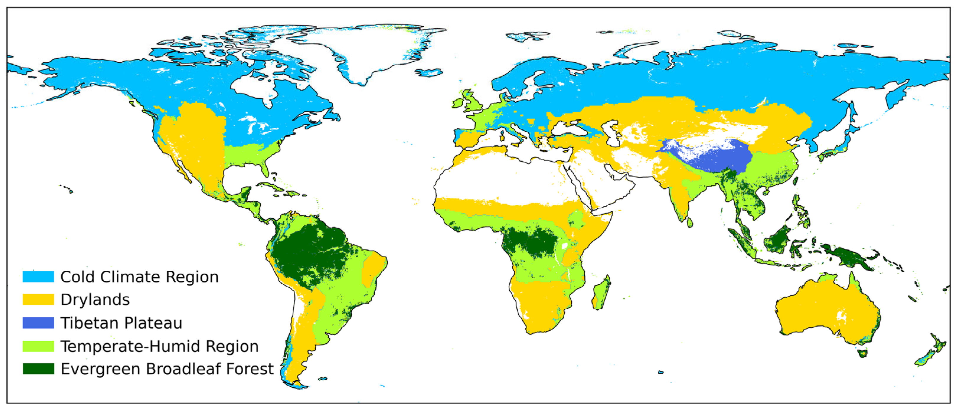
In this study, we reclassified the globe into five subregions: Cold Climate Region (CCR), Drylands (Dyd), the Tibet Plateau (TP), Temperate-Humid Region (THR), and Evergreen Broadleaf Forest (EBF). The CCR refers to the cold climates within the KG climate zones. The TP is based on the boundary of the Qinghai–Tibet Plateau. The area between 56°N and 56°S with an Aridity Index (AI) ranging from 0 to 0.65 was designated as Dyd, and the aridity gradient and arid–humid region distribution are shown in Figure S3.

The AI is calculated using the following formula:

$$\mathrm{A}\mathrm{I}={\displaystyle \frac{\sum _{\mathrm{i}=1}^{30}\frac{{\mathrm{P}}_{\mathrm{i}}}{{\mathrm{P}\mathrm{E}\mathrm{T}}_{\mathrm{i}}}}{30}},$$

(2)

where P and PET are the annual precipitation (mm year⁻¹) and potential evapotranspiration (mm year⁻¹) for 30 years (1993–2022), and i represents a specific year within the 30 years.

EBF was derived from the MCD12C1 IGBP classification and treated as an independent category. The remaining areas were classified as THRs, based on KG temperate climate zones and AI-defined humidity areas. The classification is illustrated in Figure 1.

Figure 1. The five subregions of the globe.

2.2.2. Anomaly

To eliminate the influence of seasonal cycle and investigate the responses of vegetation to environmental factors, Equation (3) was frequently used to compute the anomaly values of variables [4,17,32].

$${\mathrm{A}}_{\mathrm{i}\mathrm{j}}={\displaystyle \frac{{\mathrm{X}}_{\mathrm{i}\mathrm{j}}-\overline{{\mathrm{X}}_{\mathrm{i}}}}{{\mathsf{\sigma }}_{\mathrm{i}}}},$$

(3)

where ${\mathrm{A}}_{\mathrm{i}\mathrm{j}}$ is the anomaly value of variable X, and ${\mathrm{X}}_{\mathrm{i}\mathrm{j}}$ is X on the i^th month of the j^th year. $\overline{{\mathrm{X}}_{\mathrm{i}}}$ and ${\mathsf{\sigma }}_{\mathrm{i}}$ are the mean and standard deviation of X on the i^th month of all years. We obtained the anomalies of the three NDVI products, RSM, and SIF via the above equation.

2.2.3. Coefficient of Determination and Root Mean Square Error

This study employed a direct verification method to assess the similarity of the mean NDVI values among the NDVI_3g+, NDVI_pku, and NDVI_mod products across the five subregions from 2001 to 2022. The coefficient of determination (R²) was used to measure the degree of linear fit in scatter plots (indicating similarity), and the Root Mean Square Error (RMSE) represented the associated error.

$${\mathrm{R}}^2=1-{\displaystyle \frac{\sum _{\mathrm{i}=1}^{\mathrm{N}}{\left({\mathrm{N}\mathrm{D}\mathrm{V}\mathrm{I}}_{\mathrm{m}\mathrm{i}}-{\mathrm{N}\mathrm{D}\mathrm{V}\mathrm{I}}_{\mathrm{n}\mathrm{i}}\right)}^2}{\sum _{\mathrm{i}=1}^{\mathrm{N}}{\left({\mathrm{N}\mathrm{D}\mathrm{V}\mathrm{I}}_{\mathrm{m}\mathrm{i}}-{\overline{\mathrm{N}\mathrm{D}\mathrm{V}\mathrm{I}}}_{\mathrm{m}\mathrm{i}}\right)}^2}},$$

(4)

$$\mathrm{R}\mathrm{M}\mathrm{S}\mathrm{E}=\sqrt[2]{{\displaystyle \frac{\sum _{\mathrm{i}=1}^{\mathrm{N}}{\left({\mathrm{N}\mathrm{D}\mathrm{V}\mathrm{I}}_{\mathrm{m}\mathrm{i}}-{\mathrm{N}\mathrm{D}\mathrm{V}\mathrm{I}}_{\mathrm{n}\mathrm{i}}\right)}^2}{\mathrm{N}}}},$$

(5)

where N is the sample number, and NDVI_m and NDVI_n represent a pair from the combinations NDVI_pku, NDVI_3g+; NDVI_mod, NDVI_3g+; and NDVI_mod, NDVI_pku.

2.2.4. Theil–Sen Slope and Mann–Kendall Test

For the analysis of annual NDVI trends, we employed the non-parametric Theil–Sen slope estimator in conjunction with the Mann–Kendall (MK) trend test. The Theil–Sen estimator quantifies the trend magnitude by calculating the median of slopes between all possible pairs of data points in the time series, ensuring robustness against outliers and non-normal data distributions. The statistical significance of this trend was then determined using the MK test, a rank-based procedure that evaluates whether a monotonic upward or downward trend is statistically significant. The integration of the Theil–Sen estimator for magnitude and the MK test for significance provides a powerful and widely recognized framework for trend analysis in environmental data. The statistical significance of the trends, assessed by the MK test, was determined at a p < 0.05 significance level (corresponding to a 95% confidence interval). This widely accepted threshold was applied on a per-pixel basis across the global datasets to ensure the robustness of our conclusions.

2.2.5. Pearson Correlation Coefficient

To quantify the strength of associations between variables, the Pearson correlation coefficient (r) was employed. This metric, commonly applied in ecological and climate studies, is defined as follows:

$$\mathrm{r}\left(\mathrm{x},\mathrm{y}\right)={\displaystyle \frac{\sum _{\mathrm{i}=1}^{\mathrm{n}}\left[\left({\mathrm{x}}_{\mathrm{i}}-\overline{\mathrm{x}}\right)\times \left({\mathrm{y}}_{\mathrm{i}}-\overline{\mathrm{y}}\right)\right]}{\sqrt{\sum _{\mathrm{i}=1}^{\mathrm{n}}{\left({\mathrm{x}}_{\mathrm{i}}-\overline{\mathrm{x}}\right)}^2}\times \sqrt{\sum _{\mathrm{i}=1}^{\mathrm{n}}{\left({\mathrm{y}}_{\mathrm{i}}-\overline{\mathrm{y}}\right)}^2}}},$$

(6)

where $\overline{\mathrm{x}}$ and $\overline{\mathrm{y}}$ are the mean of $\mathrm{x}$ and $\mathrm{y}$. n is the number of samples. In this study, r was used to assess the capability of the three NDVI products in tracking seasonal cycles and anomalies in photosynthetic activity.

2.2.6. Kernel NDVI

The kernel NDVI (kNDVI) was developed by Camps-Valls et al. [33], defined in Hilbert spaces, and it adopts the radial basis function reproducing kernel. It can be described as follows:

$$\mathrm{k}\left(\mathrm{N}\mathrm{I}\mathrm{R},\mathrm{r}\mathrm{e}\mathrm{d}\right)=\mathrm{e}\mathrm{x}\mathrm{p}\left(-{\displaystyle \frac{{\left(\mathrm{N}\mathrm{I}\mathrm{R}-\mathrm{r}\mathrm{e}\mathrm{d}\right)}^2}{2{\mathsf{\sigma }}^2}}\right),$$

(7)

where $\sigma$ controls the notion of distance between the NIR and red bands. According to the definition of the kernel function, the kNDVI can be simplified as follows:

$$\mathrm{k}\mathrm{N}\mathrm{D}\mathrm{V}\mathrm{I}=\mathrm{t}\mathrm{a}\mathrm{n}\mathrm{h}\left({\left({\displaystyle \frac{\mathrm{N}\mathrm{I}\mathrm{R}-\mathrm{r}\mathrm{e}\mathrm{d}}{2\mathsf{\sigma }}}\right)}^2\right),$$

(8)

where $\mathsf{\sigma }$ is a length-scale parameter to be specified in each particular application.

Following the recommendation of the creators, we calculated the kNDVI using $\mathsf{\sigma }=0.5\left(\mathrm{N}\mathrm{I}\mathrm{R}+\mathrm{r}\mathrm{e}\mathrm{d}\right)$, which leads to a simplified operational index version expressed as follows:

$$\mathrm{k}\mathrm{N}\mathrm{D}\mathrm{V}\mathrm{I}=\mathrm{t}\mathrm{a}\mathrm{n}\mathrm{h}\left({\mathrm{N}\mathrm{D}\mathrm{V}\mathrm{I}}^2\right),$$

(9)

In this study, the three NDVI products (NDVI_3g+, NDVI_pku, and NDVI_mod) were converted into corresponding kNDVIs (kNDVI_3g+, kNDVI_pku, and kNDVI_mod).

2.3. Overall Research Procedure

This study spanned the period from March 2000 to December 2022, with a monthly temporal resolution and a spatial resolution of 0.1°. First, the time series data for all variables (i.e., the three NDVI products, RSM, and SIF) were smoothed using the Savitzky–Golay filter to eliminate outliers [34]. To ensure the analysis focused solely on vegetated surfaces, pixels where the mean NDVI value was less than 0.1 in all three NDVI datasets were masked out as non-vegetated. We intersected the images for each month to ensure a consistent number of pixels across the datasets. The evaluation of NDVI values was conducted based on the mean values over the whole study period. Spatial annual trends were examined globally via the Theil–Sen slope and MK trend test, and trend dynamics were further analyzed for individual subregions.

We obtained the anomalies of the three NDVI products, RSM, and SIF by removing the seasonal cycle using Equation (3). Subsequently, by subtracting the linear trend from the anomaly time series across each pixel involved in the calculation, we eliminated the impacts of long-term trends. Following the approach of Maurer et al. and Zeng et al. [35,36], the overall response of the NDVI to RSM is quantified by the regression coefficient (∂NDVI/∂RSM) of linear regression between detrended NDVI and RSM anomalies, with the NDVI as the dependent variable and RSM as the independent variable. For instance, the sign of ∂NDVI_3g+/∂RSM indicates the response direction of the NDVI to RSM. A positive ∂NDVI_3g+/∂RSM at a given pixel signifies that NDVI_3g+ positively responds to RSM at that location. The absolute value of ∂NDVI_3g+/∂RSM reflects the corresponding response speed (hereafter sensitivity), and a higher absolute value indicates greater sensitivity. A 95% confidence interval (i.e., p < 0.05) was applied to the regression to define statistical significance.

Furthermore, to quantitatively evaluate the capability of the three NDVI products in tracking vegetation photosynthesis, we calculated the correlation coefficients between the three NDVI products and SIF based on the time series of both the original and detrended anomalies. This approach allows for assessments of their performance in tracking seasonal cycles and anomalies in photosynthetic activity. NDVI_3g+, NDVI_pku, and NDVI_mod are transformed into the respective kNDVIs (i.e., kNDVI_3g+, kNDVI_pku, and kNDVI_mod) by Equation (9), and the mentioned correlations between kNDVIs and SIF were calculated to investigate whether the kNDVI provides an improvement over the NDVI in tracking terrestrial vegetation photosynthesis activity. A 95% confidence interval was also used to define statistical significance. In all maps, water, ice/snow, and bare ground are masked by white.

3. Results

3.1. Comparison Between NDVI_3g+, NDVI_pku, and NDVI_mod in Values

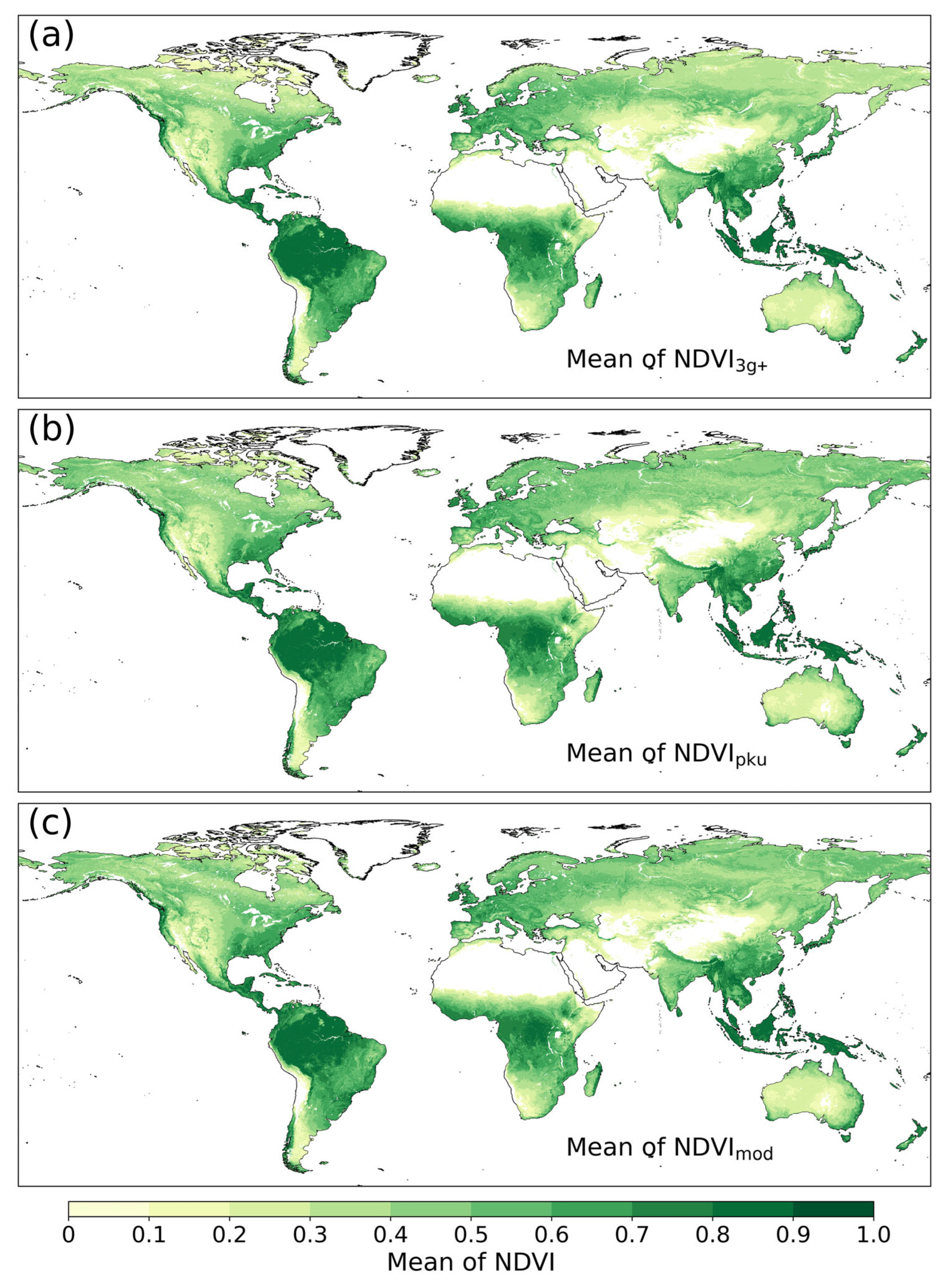
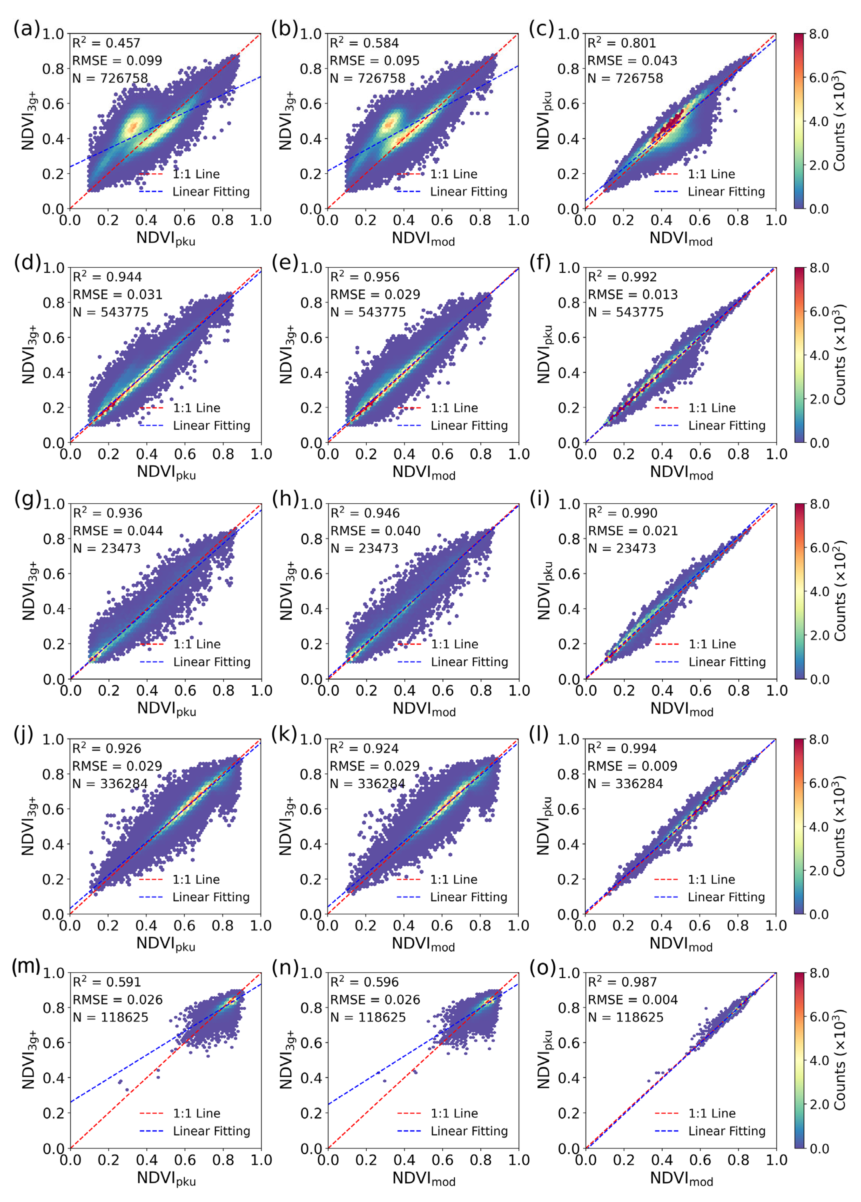
Figure 2 displays the spatial distribution of mean values for the three NDVI products over the globe. The results indicate that the patterns in the mean values of the three NDVI products are generally similar. Specifically, their values are generally higher in tropical latitudes, while they are consistently lower in arid regions. However, differences in NDVI_3g+ with NDVI_pku and NDVI_mod appear in the middle and high latitudes of the Northern Hemisphere. Consequently, we conducted a consistency assessment of their mean values across the five subregions (Figure 3). The results reveal that in the CCR, NDVI_3g+ shows low consistency with both NDVI_pku and NDVI_mod (R² = 0.457 and 0.584, respectively). In Dyd, TP, and THR, the three NDVI products show closer mean values to each other, with R² values exceeding 0.92. In EBF, NDVI_3g+ has lower consistency with NDVI_pku and NDVI_mod (R² = 0.591 and 0.596, respectively), which is similar to the situation in the CCR. For NDVI_pku and NDVI_mod, their mean values have high agreement in the Dyd, TP, THR, and EBF areas, with R² values close to 0.99, while moderate differences remain in the CCR (R² = 0.801).

Figure 2. The mean values of NDVI_3g+, NDVI_pku, and NDVI_mod. (a–c): The spatial distributions of NDVI_3g+, NDVI_pku, and NDVI_mod mean values, respectively.

Figure 3. Pairwise scatter plots of NDVI_3g+, NDVI_pku, and NDVI_mod. (a–c): Cold Climate Region (CCR); (d–f): Drylands (Dyd); (g–i): the Tibet Plateau (TP); (j–l): Temperate-Humid Region (THR); and (m–o): Evergreen Broadleaf Forest (EBF).

3.2. Annual Trend Variations Among NDVI_3g+, NDVI_pku, and NDVI_mod

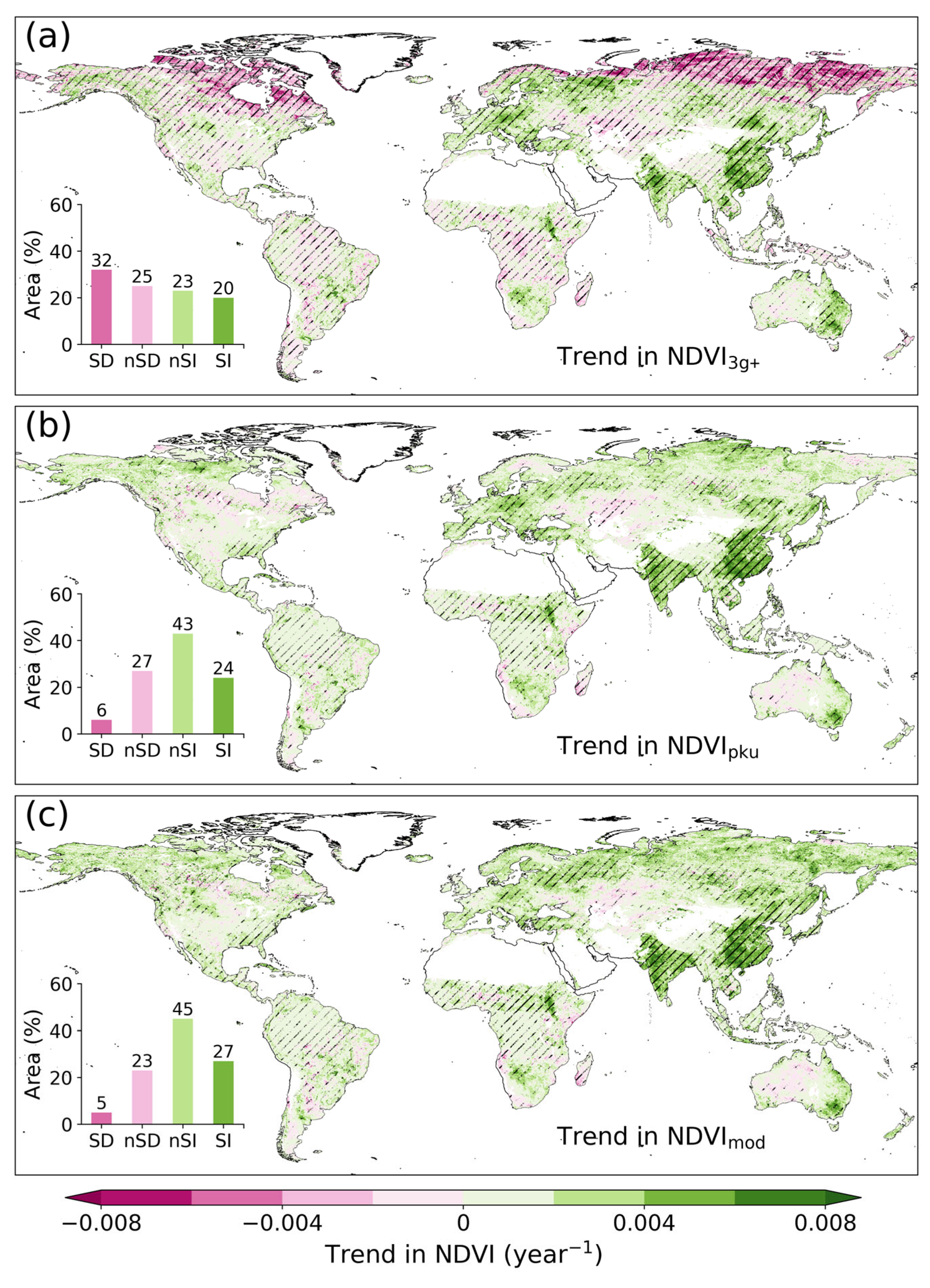
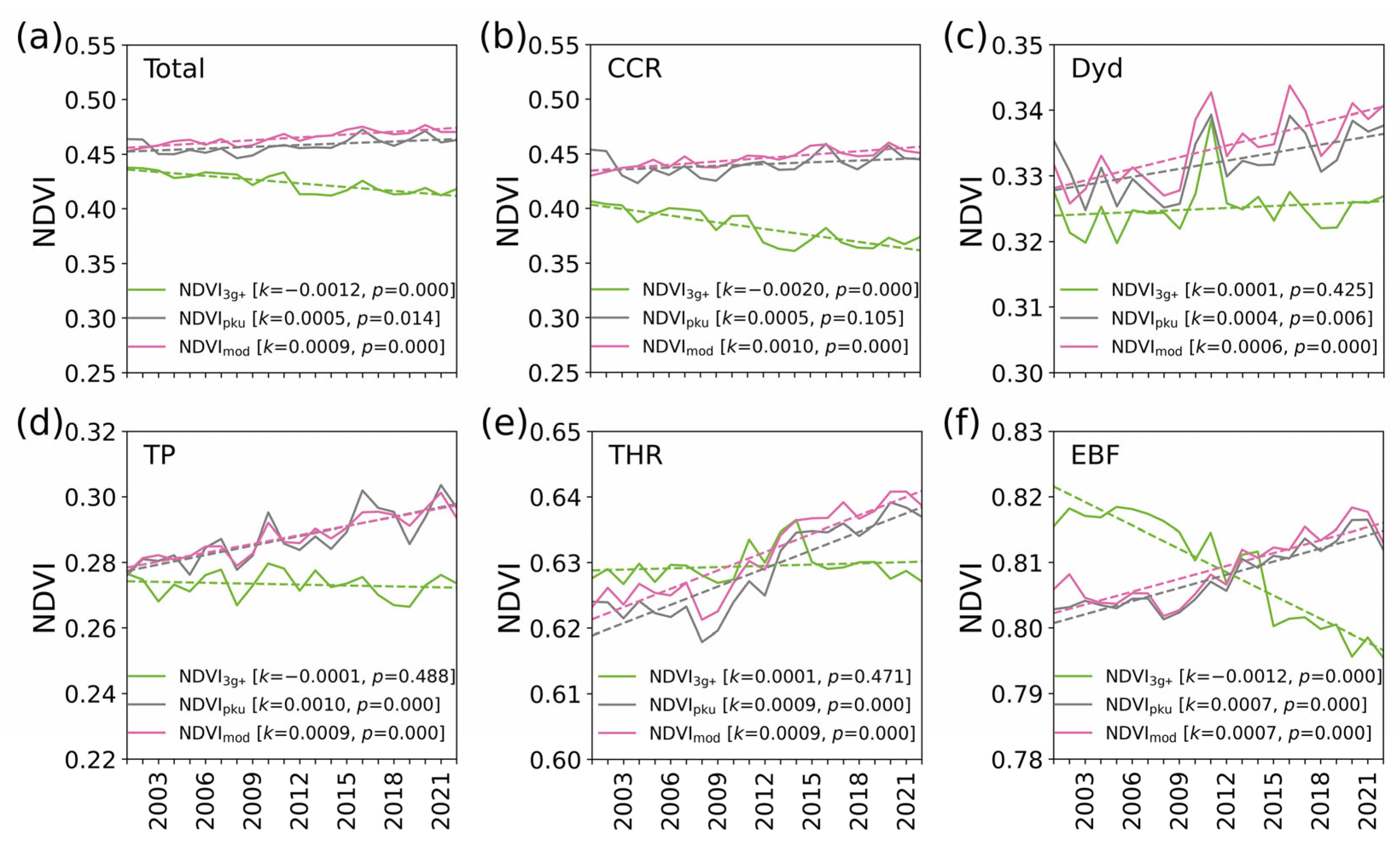
This study compares the spatial distribution of annual trends among the NDVI_3g+, NDVI_pku, and NDVI_mod products globally (Figure 4) and analyzes their annual dynamics across subregions (Figure 5). Overall, all three NDVI products reveal significant greening trends in many areas, such as Europe, eastern China, the Indian subcontinent, southern and northern Africa, and eastern Australia. The spatial distribution of annual trends in NDVI_pku and NDVI_mod are more similar to each other, whereas NDVI_3g+ shows considerable differences from both, particularly in the high latitudes of the Northern Hemisphere, EBF, central–western Kazakhstan, and Central Africa. Specifically, NDVI_3g+ demonstrates a notable browning trend in these areas, while NDVI_pku and NDVI_mod indicate a greening trend. Their annual trend differences are also reflected in the proportions of areas. NDVI_3g+ shows that 57% of the area is undergoing a browning trend (32% significant), and 43exhibits a greening trend (20% significant). NDVI_pku indicates that 33% of the area has a browning (6% significant) trend, while 67% shows the greening (24% significant) trend. NDVI_mod reflects a similar pattern to NDVI_pku, with 28% of the area browning (5% significant) and 72% greening (27% significant). This suggests that NDVI_pku and NDVI_mod exhibit similar global-scale annual trend patterns, and their proportions differ substantially from NDVI_3g+.

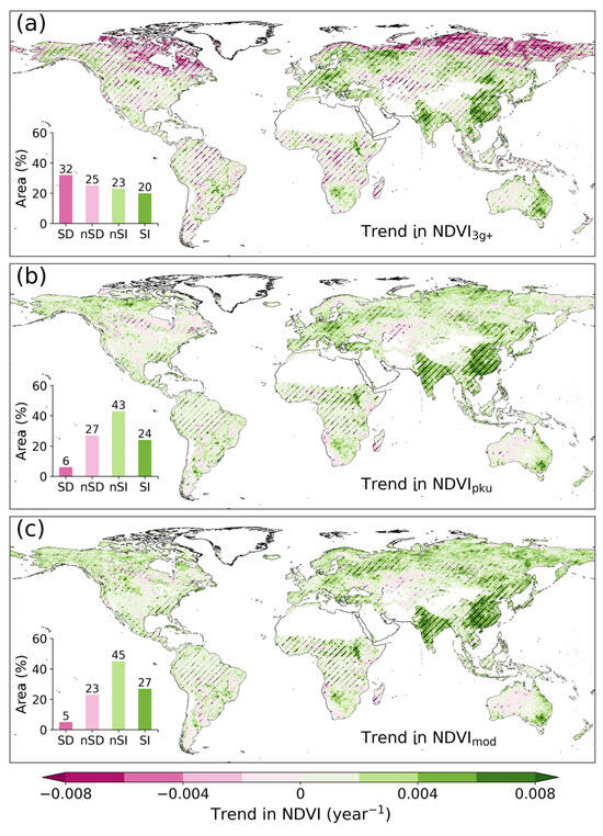
Figure 4. The annual trends in NDVI_3g+, NDVI_pku, and NDVI_mod. (a–c): The annual trend spatial distributions and the corresponding area proportions (bar plots) of NDVI_3g+, NDVI_pku, and NDVI_mod. The slash indicates the area passing the significant test (i.e., p < 0.05). SD, nSD, nSI, and SI represent significant decreasing, non-significant decreasing, non-significant increasing, and significant increasing, respectively.

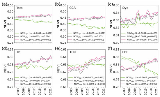
Figure 5. The annual dynamics of and trends in NDVI_3g+, NDVI_pku, and NDVI_mod. (a): the globe (Total); (b): Cold Climate Region (CCR); (c): Drylands (Dyd); (d): the Tibet Plateau (TP); (e): Temperate-Humid Region (THR); and (f): Evergreen Broadleaf Forest (EBF).

Globally, NDVI_3g+ exhibits a significant decreasing trend in annual dynamics (−0.0012 year⁻¹), whereas both NDVI_pku and NDVI_mod show significant increasing trends (0.0005 year⁻¹ and 0.0009 year⁻¹, respectively). Similar differences are observed at the regional scale in the CCR, with the significant decreasing trend in NDVI_3g+ being especially pronounced (k = −0.0020). In Dyd, all three NDVI products show an increasing trend. NDVI_pku and NDVI_mod display a significant increasing trend (0.0004 year⁻¹ and 0.0006 year⁻¹, respectively), while NDVI_3g+ shows a non-significant increasing trend (0.0001 year⁻¹, p = 0.425). In the TP, both NDVI_pku and NDVI_mod exhibit a significant increasing trend (0.0010 year⁻¹ and 0.0009 year⁻¹, respectively), whereas NDVI_3g+ shows a non-significant decreasing trend (−0.0001 year⁻¹, p = 0.488). For the THR, NDVI_pku and NDVI_mod demonstrate significant increasing (both with 0.0009 year⁻¹), whereas NDVI_3g+ shows no significant overall trend (0.0001 year⁻¹, p = 0.471); however, it initially increased before 2014 and then decreased. Over EBF, NDVI_3g+ shows a significant decreasing trend (−0.0012, year⁻¹), while NDVI_pku and NDVI_mod exhibit a significant increasing trend (both equal 0.0007 year⁻¹).

3.3. Responses of NDVI_3g+, NDVI_pku, and NDVI_mod to RSM

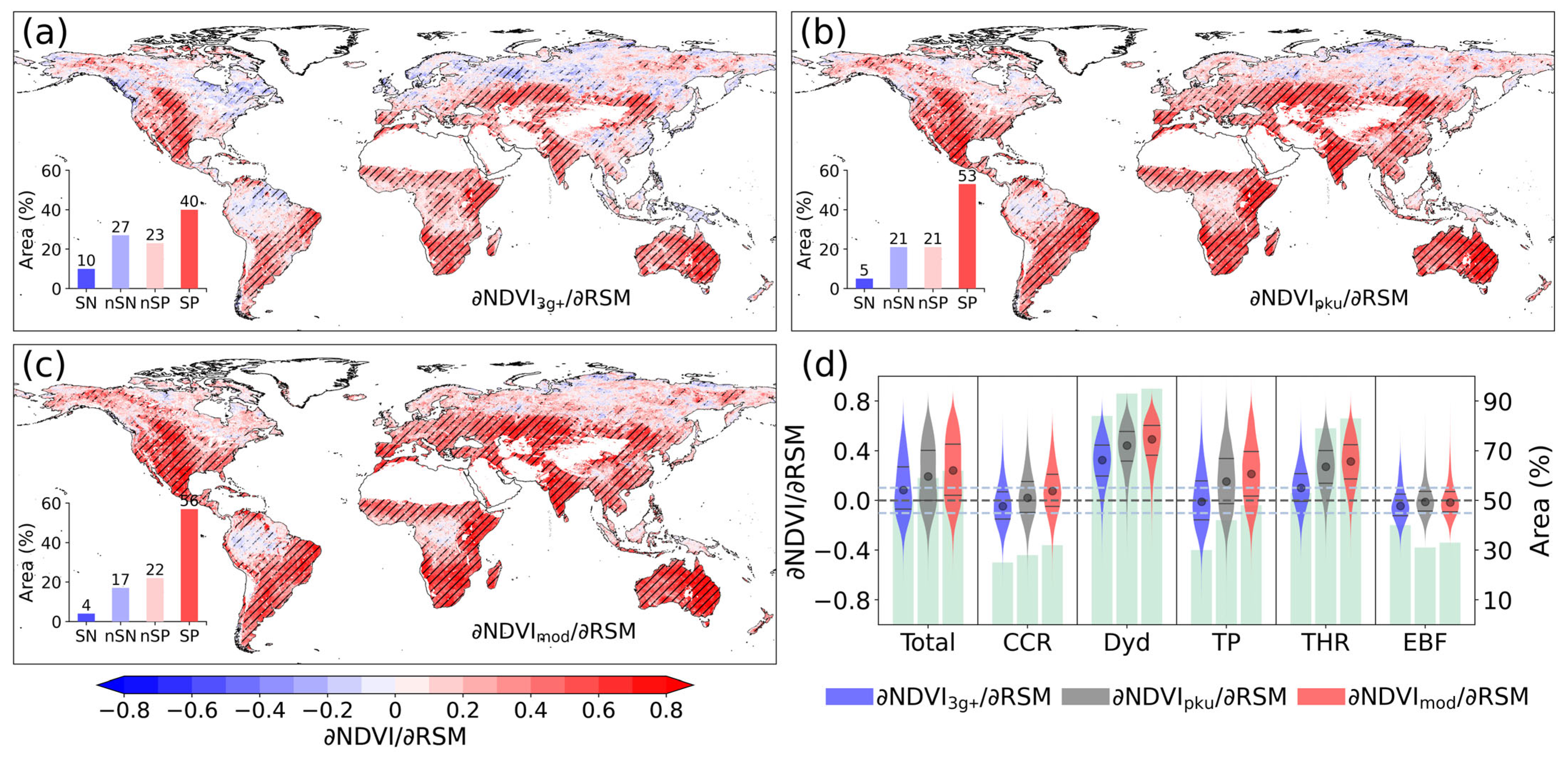
This study investigates the responses of NDVI_3g+, NDVI_pku, and NDVI_mod to RSM (∂NDVI_3g+/∂RSM, ∂NDVI_pku/∂RSM, and ∂NDVI_mod/∂RSM) over the globe. Spatially (Figure 6a–c), these three NDVI products display a positive response to RSM within Dyd. However, variability in their responses to RSM emerges across the remaining subregions. In terms of response area proportions, NDVI_3g+ exhibits a positive response to RSM across 63% of the global land area, with 40% showing significant responses, and a negative response over 37%, with 10% being significant. NDVI_pku reflects a positive response in 74% of the globe, 53% of which is significant, and a negative response in 26%, with 5% being significant. Compared to the two mentioned NDVI products, NDVI_mod shows the highest area proportion of positive responses to RSM, covering 78% of the global land area (56% significant), and the lowest proportion of negative responses, at 21% (4% significant). NDVI_3g+ demonstrates the highest proportion of negative responses to RSM on a global scale, distributed across regions outside Dyd. The negative responses of NDVI_pku and NDVI_mod are primarily concentrated in the CCR and EBF.

Figure 6. The responses of NDVI_3g+, NDVI_pku, and NDVI_mod to root-zone soil moisture (RSM). (a–c): The spatial distributions of the regression slope of NDVI_3g+, NDVI_pku, and NDVI_mod to RSM (∂NDVI_3g+/∂RSM, ∂NDVI_pku/∂RSM, and ∂NDVI_mod/∂RSM) and the corresponding area proportions (bar plots). The slash indicates the area passing the significant test (i.e., p < 0.05). SN, nSN, nSP, and SP represent the significant negative, non-significant negative, non-significant positive, and significant positive responses of the three NDVI products to RSM. (d): The statistic of the regression slopes of the three NDVI products to RSM (∂NDVI/∂RSM, violin plots) and area proportions passing the significance test (bar plots) over the globe (Total), Cold Climate Region (CCR), Drylands (Dyd), the Tibet Plateau (TP), Temperate-Humid Region (THR), and Evergreen Broadleaf Forest (EBF). The dots and short lines in the violin plots represent the median and interquartile range, respectively.

This study further examined ∂NDVI_3g+/∂RSM, ∂NDVI_pku/∂RSM, and ∂NDVI_mod/∂RSM across subregions (Figure 6d). Overall, the responses of all three NDVI products to RSM are dominantly positive (slope median > 0), and their sensitivities to RSM are at the rank of ∂NDVI_mod/∂RSM > ∂NDVI_pku/∂RSM > ∂NDVI_3g+/∂RSM. The area proportion passing the significance test follows this ranking as well. Regionally, in the CCR, all slope medians are below the significance threshold, indicating that the sensitivities of NDVI_3g+, NDVI_pku, and NDVI_mod to RSM are generally low and predominantly non-significant. Furthermore, based on slope medians, NDVI_pku and NDVI_mod show positive responses to RSM, while NDVI_3g+ exhibits primarily negative responses. In Dyd, these three NDVI products show relative consistent positive responses to RSM, with sensitivities ranked as ∂NDVI_mod/∂RSM > ∂NDVI_pku/∂RSM > ∂NDVI_3g+/∂RSM. Over the TP, the non-significant slope median in the regression of NDVI_3g+ to RSM shows a non-significant response and low sensitivity to RSM, whereas NDVI_pku and NDVI_mod show positive responses with significant median sensitivities. Within the THR, all three NDVI products predominantly respond positively to RSM, though with lower sensitivities than those over Dyd, ranked as ∂NDVI_mod/∂RSM > ∂NDVI_pku/∂RSM > ∂NDVI_3g+/∂RSM. In the EBF, all the three NDVI products show great uncertainties in response to RSM, dominating in non-significant response. Additionally, across the CCR, Dyd, TP, and THR, the area proportion passing the significance test ranks as ∂NDVI_mod/∂RSM > ∂NDVI_pku/∂RSM > ∂NDVI_3g+/∂RSM, with lower proportions in the CCR and TP (below 50%) and the highest proportion in Dyd (above 80%).

3.4. Seasonality and Anomaly Consistencies of NDVI_3g+, NDVI_pku, and NDVI_mod with SIF

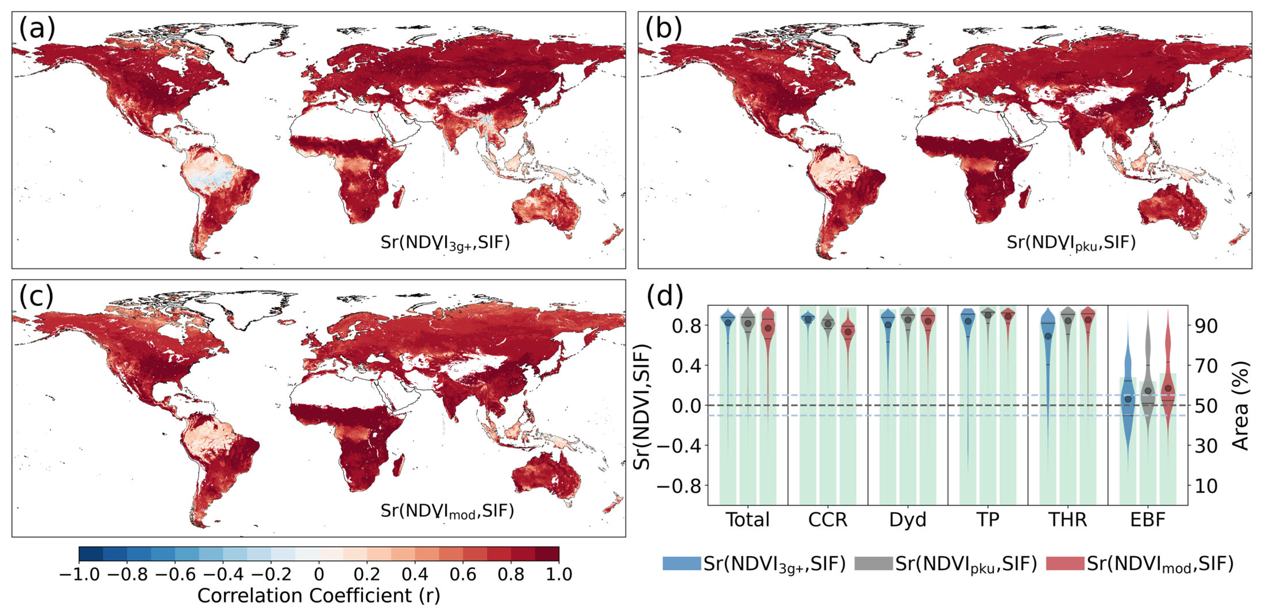
This study assesses the ability of NDVI_3g+, NDVI_pku, and NDVI_mod to represent terrestrial vegetation activity and productivity by examining the consistency of the three NDVI products with SIF in terms of seasonality and anomaly. Figure 7 illustrates the spatial seasonality correlations between the three NDVI products and SIF (Sr(NDVI_3g+, SIF), Sr(NDVI_pku, SIF), and Sr(NDVI_mod, SIF)), accompanying statistical analyses over subregions. Overall, all three NDVI products exhibit strong seasonality correlations with SIF. However, the correlations are notably lower in the EBF, with NDVI_3g+ even showing negative correlations in southeastern China and the Amazon. The strength of the overall seasonality correlations follows the order of Sr(NDVI_3g+, SIF) > Sr(NDVI_pku, SIF) > Sr(NDVI_mod, SIF) (Figure 7d). A similar pattern is observed over the CCR. However, in Dyd, TP, and THR, Sr(NDVI_pku, SIF) and Sr(NDVI_mod, SIF) are comparable, and both are stronger than Sr(NDVI_3g+, SIF). All the area proportions passing the significance test in such regions are greater than 95%. In the EBF, Sr(NDVI_3g+, SIF), Sr(NDVI_pku, SIF), and Sr(NDVI_mod, SIF) are noticeably lower compared to those in other subregions, as well as the area proportion passing the significance test.

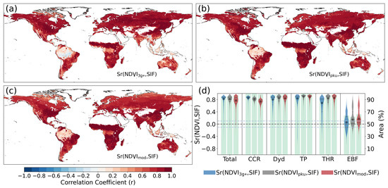
Figure 7. The seasonality consistencies of NDVI_3g+, NDVI_pku, and NDVI_mod with SIF. (a–c): The spatial distributions of seasonality correlation between NDVI_3g+, NDVI_pku, and NDVI_mod and SIF (Sr(NDVI_3g+, SIF), Sr(NDVI_pku, SIF), and Sr(NDVI_mod, SIF)), only showing the area passing the significance test. (d): The statistics of the seasonality correlation between the three NDVI products and SIF (Sr(NDVI, SIF), violin plots), along with the area proportion passing the significance test (bar plots), over the globe (Total), Cold Climate Region (CCR), Drylands (Dyd), the Tibet Plateau (TP), Temperate-Humid Region (THR), and Evergreen Broadleaf Forest (EBF). The dots and short lines in the violin plots represent the median and interquartile range, respectively.

Figure 8 illustrates spatial anomaly correlations between NDVI_3g+, NDVI_pku, and NDVI_mod and SIF (Ar(NDVI_3g+, SIF), Ar(NDVI_pku, SIF), and Ar(NDVI_mod, SIF)) (Figure 8a–c), along with their statistical summaries (Figure 8d). Spatially, Ar(NDVI_pku, SIF) and Ar(NDVI_mod, SIF) are greater than Ar(NDVI_3g+, SIF), which means the anomalies of NDVI_pku and NDVI_mod show a closer linkage to that of SIF. Higher correlations are concentrated in Dyd, while lower correlations are mainly observed in the CCR and EBF. The aggregated statistics reveal that, overall, Ar(NDVI_pku, SIF) is the strongest, followed by Ar(NDVI_mod, SIF), with Ar(NDVI_3g+, SIF) being the weakest. Additionally, the area proportion passing the significance test exceeds 85%. A similar pattern is observed in the CCR. In Dyd, TP, and THR, Ar(NDVI_pku, SIF) and Ar(NDVI_mod, SIF) are similar, and both exceed Ar(NDVI_3g+, SIF). Over the EBF, the anomaly correlations follow the order of Ar(NDVI_mod, SIF) > Ar(NDVI_pku, SIF) > Ar(NDVI_3g+, SIF), but they are lower than those in other regions. Notably, over Dyd, both spatial correlation patterns and regional statistics confirm that the NDVI anomalies align more closely with SIF anomalies. Moreover, for Ar(NDVI_3g+, SIF), the area proportion passing the significance test is always lower than that of Ar(NDVI_pku, SIF) and Ar(NDVI_mod, SIF), particularly in the TP and EBF.

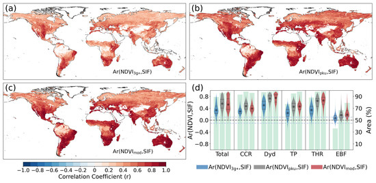
Figure 8. The anomaly consistency of NDVI_3g+, NDVI_pku, and NDVI_mod with SIF. (a–c): The spatial distributions of anomaly correlations between NDVI_3g+, NDVI_pku, and NDVI_mod and SIF (Ar(NDVI_3g+, SIF), Ar(NDVI_pku, SIF), and Ar(NDVI_mod, SIF)), only showing the area passing the significance test. (d): The statistics of the anomaly correlations between the three NDVI products and SIF (Ar(NDVI, SIF), violin plots), along with the area proportion passing the significance test (bar plots), over the globe (Total), Cold Climate Region (CCR), Drylands (Dyd), the Tibet Plateau (TP), Temperate-Humid Region (THR), and Evergreen Broadleaf Forest (EBF). The dots and short lines in the violin plots represent the median and interquartile range, respectively.

4. Discussion

4.1. The Sources of Inter-Product Variability Among the Three NDVI Products

The discrepancies in the source data and methods used to generate the NDVI datasets are likely the primary reasons for the observed differences between the three NDVI products. Specifically, NDVI_3g+ utilizes the red (550–680 nm) and NIR (725–1100 nm) bands from NOAA sensors. The series of NOAA sensors undergo frequent updates [24,26]. NDVI_mod, based on MODIS sensors, uses the red (620–670 nm) and NIR (841–876 nm) bands.

The broader wavelength range of NOAA sensors makes them more vulnerable to interference from atmospheric components such as water vapor [37], aerosols [38], and snow [39], which is challenging to accurately remove. On the other hand, the narrower wavelength range of MODIS sensors enhances their sensitivity to chlorophyll [40]. The wavelength range of the sensors is one of the key factors contributing to the differences between NDVI_3g+ and NDVI_mod and is also likely a contributing factor behind the observed Ar(NDVI_mod, SIF) > Ar(NDVI_3g+, SIF) (Figure 8). Additionally, NOAA sensors have undergone frequent replacements, leading to variations in overpass times and orbital drift. Despite the application of correction techniques such as empirical mode decomposition and Bayesian adjustment approaches [24], the NDVI_3g+ dataset still retains a degree of residual uncertainty and signal noise, particularly in regions and periods affected by sensor degradation and atmospheric interference. In contrast, the MODIS sensor, despite showing signs of aging, has not been replaced.

We also considered local observational time as a potential factor, given the distinct overpass times of the platforms (AVHRR: 2:30 AM/PM; Terra MODIS/Landsat: 11 AM/PM). To test this, we systematically evaluated NDVI_aqu (1:30 PM/AM) across multiple dimensions: mean value, trends, sensitivity to RSM, and consistency with SIF (Figures S4–S7). The results robustly demonstrate that NDVI_aqu aligns more closely with NDVI_pku and NDVI_mod than with NDVI_3g+, indicating that overpass time is not the primary cause of the observed discrepancies.

During the overlapping period (2003–2015), NDVI_pku was generated by fusing GIMMS v1.0 NDVI and MODIS NDVI on the pixel scale using an 11 × 11 moving window and the random forest algorithm. However, both our results and those of Li et al. (2023) indicate that NDVI_pku is closer to NDVI_mod in terms of values and annual trends [18]. This is likely due to the cross-calibration conducted during the production of NDVI_pku using approximately 3.6 million Landsat NDVI samples.

Additionally, over the EBF, the three NDVI products exhibit notable differences in their values and annual trends, and they show non-significant responses and low sensitivity to RSM, as well as weak seasonality and anomaly correlations with SIF, accompanied by considerable uncertainties. This can be attributed to the inherent tendency of the NDVI to saturate in such areas with high canopy density, a characteristic that may limit the ability to accurately capture vegetation information in EBF [41].

4.2. Potential Impacts and Applications

Our results highlight differences in NDVI values between NDVI_3g+ and both NDVI_pku and NDVI_mod within the CCR and EBF. Similar discrepancies have been noted in previous studies [20,21]. This could be attributed to the aforementioned data sources and production methods. It could also be caused by the effects of snow cover and the saturation of the NDVI over such regions [39,42]. As canopy density increases, the NDVI asymptotically approaches an upper limit, making its ability to characterize vegetation information weaker. This saturation effect could explain why the NDVI has a limited capability to capture both vegetation activity and variations in canopy greenness [43,44,45] and shows less sensitivity to water availability fluctuations in forests [4,17]. To overcome the limitations of the NDVI, alternative vegetation indices have been developed. The Enhanced Vegetation Index (EVI), for instance, was specifically designed to reduce saturation effects by incorporating the blue band for aerosol correction, resulting in a greater dynamic range and improved sensitivity over high-biomass regions [46,47]. Similarly, the Photochemical Reflectance Index (PRI), which is sensitive to changes in xanthophyll cycle pigments, has shown promise in tracking light-use efficiency and physiological stress in evergreen canopies [48,49]. These differences have affected research areas that depend on NDVI values, such as terrestrial productivity estimation [50], vegetation type classification [51], and vegetation coverage assessments [52].

Trends from NDVI_pku and NDVI_mod align with the findings of Li et al. [18]. Although the temporal coverage of GIMMS NDVI used in this study differs from that in other studies, partly explaining the discrepancies in GIMMS NDVI trends, a more significant observation is that both our study and previous studies consistently reveal notable differences in trends between GIMMS NDVI and MODIS NDVI [21,53,54]. Actually, other vegetation indicators, such as the LAI [55], SIF [56], and gross primary productivity [57,58], suggest an overall global greening trend or increases in vegetation productivity. Recent research using various datasets has revealed conflicting vegetation trends in nearly half of the global regions and highlighted that such differences are likely linked to data processing algorithms [54]. However, the significant browning trend indicated by NDVI_3g+, which contrasts with other indicators, still warrants careful consideration. This not only underscores the considerable uncertainties and potential challenges in monitoring vegetation dynamics under climate change using different datasets but also emphasizes the critical importance of employing multiple vegetation indicators to analyze global greening and browning trends.

The three NDVI products exhibited large areas of non-significant or significantly negative responses to RSM over the CCR. Similar findings have been reported in studies by Liu et al. [4]. This is likely due to the fact that the vegetation growth in the CCR is dominated by energy-related variables [59,60] and affected by water logging and water surplus [17,61]. Additionally, in the CCR, TP, and THR, NDVI_3g+ shows notable differences from NDVI_pku and NDVI_mod in response to RSM, which suggests that caution is necessary when interpreting NDVI responses to environmental stress factors over such regions. Incorporating more observational data or using multiple vegetation indicators could be a more reasonable and effective approach for further studies.

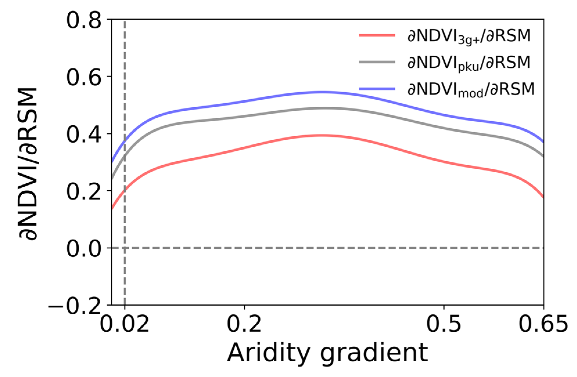
We also observed a high consistency in their responses to RSM in Dyd, predominantly characterized by positive responses. This suggests that vegetation growth in Dyd is primarily driven by water supply, a finding that aligns with previous studies [4,17,62]. Consequently, we examined the variation in their sensitivity across the aridity gradient in Dyd (Figure 9). The results show that the sensitivity of the three NDVI products to RSM increases initially and then decreases, maintaining the order of ∂NDVI_mod/∂RSM > ∂NDVI_pku/∂RSM > ∂NDVI_3g+/∂RSM. This is consistent with the findings of previous studies [4]. These results are crucial for selecting the appropriate NDVI product (i.e., NDVI_mod) when studying vegetation responses and sensitivities to water stress factors and drought in Dyd.

Figure 9. The sensitivities of NDVI_3g+, NDVI_pku, and NDVI_mod to root-zone soil moisture (RSM) across aridity gradients (0 < Aridity Index < 0.65) over the Drylands (Dyd) within 56°N~56°S.

The findings of this study provide important insights for ecosystem monitoring and decision making. For carbon accounting, if the global browning trend shown by NDVI_3g+ is adopted, it may lead to significant deviations in the estimation of the global terrestrial carbon sink compared to results based on NDVI_pku or NDVI_mod. This highlights the critical importance of carefully selecting vegetation index products when building global carbon budget models. For drought early warning, our results show that NDVI_mod has the highest sensitivity to RSM in Drylands, suggesting that integrating NDVI_mod into existing drought monitoring systems could enable a more timely and accurate detection of vegetation water stress, thereby enhancing early warning capabilities. For SDG monitoring, particularly when assessing vegetation dynamics and their responses to climate change in vulnerable biomes, discrepancies among NDVI products could lead to differing conclusions. Therefore, based on our study, we recommend prioritizing the use of products with higher consistency across multiple vegetation indicators (such as NDVI_pku and NDVI_mod) to enhance the reliability and comparability of monitoring results and provide a more solid scientific basis for relevant policy formulation and evaluation.

Seasonality information regarding the NDVI is often used to extract vegetation phenology [63] and growing season characteristics [64]. We thus analyzed the seasonality consistency of the three NDVI products with SIF. Figure 7 indicates that in the EBF, the three NDVI products exhibit low seasonality consistency with SIF. Aside from the susceptibility of the NDVI to saturation, the absence of distinct seasonal variations in EBF vegetation is also a significant contributing factor. Figure 8 shows that Ar(NDVI_pku, SIF) and Ar(NDVI_mod, SIF) are higher than Ar(NDVI_3g+, SIF), suggesting that NDVI_pku and NDVI_mod are more suitable for representing the anomaly dynamics of terrestrial vegetation activity and productivity.

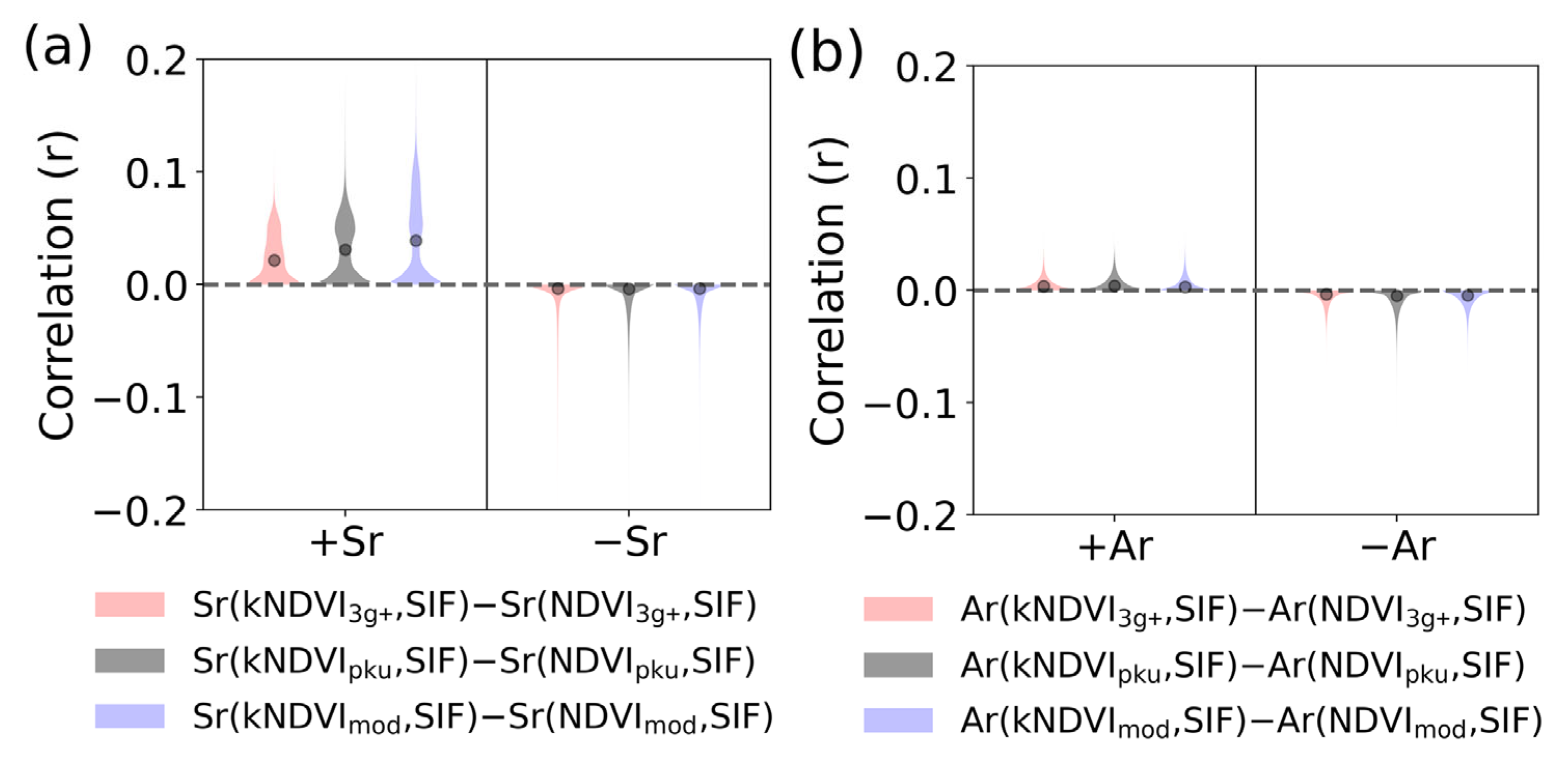
Among the NDVI-based extended indices, the kNDVI stands out as one of the most effective [33]. We converted the three NDVI products to kNDVIs and analyzed the difference between Sr(kNDVI, SIF) and Sr(NDVI, SIF) and that between Ar(kNDVI, SIF) and Ar(NDVI, SIF) (Figure 10), with the spatial seasonality and anomaly correlations of the kNDVI with SIF and their differences shown in Figures S8–S10. The results indicate that, compared to the NDVI, the seasonality alignment between the kNDVI and SIF has improved in approximately 85% of global areas, with notable improvements concentrated in the middle and high latitudes. This suggests that the kNDVI might be a superior choice for estimating terrestrial productivity and extracting vegetation phenology and growing season characteristics. This also supports recent studies in related fields utilizing the kNDVI [65,66]. Figure 10 and Figure S10 also imply that the anomaly consistency of the kNDVI with SIF did not show notable improvement. Therefore, to capture the anomaly dynamics of terrestrial vegetation activity and productivity, the kNDVI performs nearly identically to the NDVI.

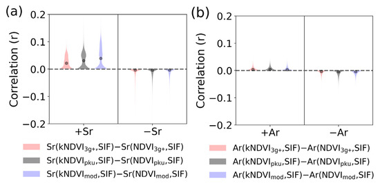
Figure 10. The statistic of difference between the kNDVI and NDVI in seasonality and anomaly consistencies with SIF. (a): Violin plots of the difference in the seasonality correlation between the kNDVI and SIF versus the NDVI and SIF ((a): Sr(kNDVI_3g+, SIF)-Sr(NDVI_3g+, SIF), Sr(kNDVI_pku, SIF)-Sr(NDVI_pku, SIF), and Sr(kNDVI_mod, SIF)-Sr(NDVI_mod, SIF)). (b): Violin plots of the difference in the anomaly correlation between the kNDVI and SIF versus the NDVI and SIF ((a): Ar(kNDVI_3g+, SIF)-Ar(NDVI_3g+, SIF), Ar(kNDVI_pku, SIF)-Ar(NDVI_pku, SIF), and Ar(kNDVI_mod, SIF)-Ar(NDVI_mod, SIF)).

This performance discrepancy is likely rooted in the intrinsic properties of the kNDVI algorithm. The kernel function is designed to better capture complex and stable vegetation structural features through nonlinear mapping, making it exceptionally effective at characterizing strong and regular seasonal cycles (a low-frequency signal). However, this mapping process introduces a temporal smoothing effect, which acts like a low-pass filter. In contrast, vegetation anomalies typically manifest as short-lived, abrupt, high-frequency signals. Consequently, while the kNDVI amplifies the dominant seasonal signal, it may inadvertently suppress the amplitude of these transient anomalous signals. This is likely the primary reason for its relatively modest improvement in tracking SIF anomalies.

Previous studies emphasized the limitations of NOAA sensors, such as the broad wavelength coverage and frequent sensor replacements, and the advantages of MODIS sensors, which include advanced calibration methods, a narrower wavelength coverage, and higher band resolution [3,38]. However, the importance of the temporal span of NDVI_3g+ is unmatched by other NDVI datasets, particularly under climate change. This underscores the significance of reconstructing NDVI products, as exemplified by NDVI_pku, which integrates high-precision Landsat NDVI data with the characteristics of both NDVI_3g+ and NDVI_mod. Future research should prioritize the integration of advantages from multi-source data to develop superior NDVI products. This is crucial for enhancing the diversity and applicability of vegetation data, particularly given the increasing significance of vegetation in the water cycle, energy cycle, and carbon exchange processes.

4.3. Limitations and Future Directions

In this study, we employed an averaging method to composite half-month data (i.e., NDVI_3g+ and NDVI_pku) to obtain a monthly temporal resolution to match the temporal resolution of NDVI_mod. This most likely causes a loss of temporal detail. The maximum NDVI value within a compositing period may be lower than the absolute physiological peak of the vegetation because it is effectively averaged with values from earlier or later in the month when the canopy was less developed, potentially leading to an underestimation of the maximum photosynthetic capacity. Furthermore, the timing of critical phenological phases, such as the start or end of the growing season, can be blurred. A rapid green-up event that occurs over a few days might be obscured within the monthly composite, making it difficult to pinpoint the exact onset date with high precision. This effect is the most pronounced in ecosystems with abrupt transitions, such as deciduous forests and croplands, where a difference of days can be ecologically significant. Therefore, in future research applying the NDVI, we will adopt a higher temporal resolution.

This study revealed substantial discrepancies, and in some cases, opposing trends, between the NDVI_3g+ product and the other two products. A primary limitation of our work is its focus on inter-product comparison rather than determining the definitive state of global vegetation trends. Consequently, our future research will prioritize a multi-faceted investigation into global vegetation dynamics by integrating diverse vegetation indicators.

5. Conclusions

In this study, we conducted a comprehensive assessment between newly released and commonly used NDVI products, including NDVI_3g+, NDVI_pku, and NDVI_mod, focusing on value, trend, response to RSM, and performance in representing vegetation activity and productivity. The results show that the three NDVI products exhibit high agreement in mean values across most areas, while NDVI_3g+ shows notable deviations from NDVI_pku and NDVI_mod in the CCR and EBF. In terms of annual trends, NDVI_3g+ indicates global significant browning (−0.0012 year⁻¹), while both NDVI_pku (0.0005 year⁻¹) and NDVI_mod (0.0009 year⁻¹) suggest global significant greening. These trend differences are also observed across all subregions, emphasizing the necessity of using diverse vegetation indicators for reliable assessments of global vegetation trends. Additionally, the responses of the three NDVI products to RSM show considerable uncertainties in the CCR, TP, and EBF. However, they display a high degree of consistency in Dyd, with sensitivities ranked as ∂NDVI_mod/∂RSM > ∂NDVI_pku/∂RSM > ∂NDVI_3g+/∂RSM. This implies that NDVI_mod could be more appropriate for studying vegetation responses to water stress and drought in such regions. Our results also show that all three NDVI products demonstrate a high seasonality consistency with SIF, except over EBF. Specifically, NDVI_3g+ shows stronger consistency with SIF in the CCR (r > 0.8), whereas NDVI_pku and NDVI_mod exhibit stronger consistency in Dyd, TP, and THR (with all r values above 0.8).

We also observed that, compared to the NDVI, the seasonality consistency between the corresponding kNDVI and SIF improves over 85% of the globe, with the most pronounced improvements occurring in the middle and high latitudes over the Northern Hemisphere. This suggests that the kNDVI holds greater promise for estimating terrestrial productivity and extracting information on vegetation phenology and growing season characteristics. Additionally, the overall anomaly consistency between NDVI products and SIF follows the order of Ar(NDVI_pku, SIF) > Ar(NDVI_mod, SIF) > Ar(NDVI_3g+, SIF). Over subregions, NDVI_pku shows the highest anomaly consistency with SIF in the CCR (r > 0.5), while NDVI_3g+ has the lowest consistency (r < 0.4). In Dyd, TP, and THR, NDVI_pku and NDVI_mod demonstrate higher anomaly consistency with SIF. The similar pattern between the kNDVI and NDVI in anomaly consistency with SIF indicates that both the NDVI and kNDVI perform closely in capturing the anomaly dynamics of terrestrial vegetation activity and productivity. Additionally, in the EBF, both the NDVI and kNDVI exhibit lower consistency with SIF in terms of seasonality fluctuations and anomaly dynamics. Our study enhances the understanding of the respective strengths and limitations among the three NDVI products and advances their potential applications in ecological sustainability under climate change. We also highlight the importance of leveraging the strengths of different NDVI datasets to develop improved and robust NDVI data.

References

- Anderegg, W.R.L.; Konings, A.G.; Trugman, A.T.; Yu, K.; Bowling, D.R.; Gabbitas, R.; Karp, D.S.; Pacala, S.; Sperry, J.S.; Sul-man, B.N.; et al. Hydraulic diversity of forests regulates ecosystem resilience during drought. Nature 2018, 561, 538–541. [Google Scholar] [CrossRef] [PubMed]
- Tucker, C.J. Red and photographic infrared linear combinations for monitoring vegetation. Remote Sens. Environ. 1979, 8, 127–150. [Google Scholar] [CrossRef]
- Zeng, Y.; Hao, D.; Huete, A.; Dechant, B.; Berry, J.; Chen, J.M.; Joiner, J.; Frankenberg, C.; Bond-Lamberty, B.; Ryu, Y.; et al. Optical vegetation indices for monitoring terrestrial ecosystems globally. Nat. Rev. Earth Environ. 2022, 3, 477–493. [Google Scholar] [CrossRef]
- Liu, Q.; Yao, F.; Garcia-Garcia, A.; Zhang, J.; Li, J.; Ma, S.; Li, S.; Peng, J. The response and sensitivity of global vegetation to water stress: A comparison of different satellite-based NDVI products. Int. J. Appl. Earth Obs. Geoinf. 2023, 120, 103341. [Google Scholar] [CrossRef]
- Piao, S.; Nan, H.; Huntingford, C.; Ciais, P.; Friedlingstein, P.; Sitch, S.; Peng, S.; Ahlström, A.; Canadell, J.G.; Cong, N.; et al. Evidence for a weakening relationship between interannual temperature variability and northern vegetation activity. Nat. Commun. 2014, 5, 5018. [Google Scholar] [CrossRef]
- Ogutu, B.O.; D’Adamo, F.; Dash, J. Impact of vegetation greening on carbon and water cycle in the African Sahel-Sudano-Guinean region. Glob. Planet. Change 2021, 202, 103524. [Google Scholar] [CrossRef]
- Yuan, W.; Liu, S.; Dong, W.; Liang, S.; Zhao, S.; Chen, J.; Xu, W.; Li, X.; Barr, A.; Andrew Black, T.; et al. Differentiating moss from higher plants is critical in studying the carbon cycle of the boreal biome. Nat. Commun. 2014, 5, 4270. [Google Scholar] [CrossRef]
- De La Guardia, L.; Miranda, J.H.D.; Luciano, A.C.d.S. Assessment of irrigation water use for dry beans in center pivots using ERA5 Land climate variables and Sentinel 2 NDVI time series in the Brazilian Cerrado. Agric. Water Manag. 2024, 305, 109128. [Google Scholar] [CrossRef]
- Feng, L.; Wang, Y.; Fensholt, R.; Tong, X.; Tagesson, T.; Zhang, X.; Ardö, J.; Zhou, J.; Shao, W.; Dou, Y.; et al. Globally increased cropland soil exposure to climate extremes in recent decades. Nat. Commun. 2025, 16, 4354. [Google Scholar] [CrossRef]
- Usman, M.; Liedl, R.; Shahid, M.A.; Abbas, A. Land use/land cover classification and its change detection using multi-temporal MODIS NDVI data. J. Geogr. Sci. 2015, 25, 1479–1506. [Google Scholar] [CrossRef]
- Faheem, Z.; Kazmi, J.H.; Shaikh, S.; Arshad, S.; Noreena; Mohammed, S. Random forest-based analysis of land cover/land use LCLU dynamics associated with meteorological droughts in the desert ecosystem of Pakistan. Ecol. Indic. 2024, 159, 111670. [Google Scholar] [CrossRef]
- Zhu, W.; Xie, Z.; Zhao, C.; Zheng, Z.; Qiao, K.; Peng, D.; Fu, Y.H. Remote sensing of terrestrial gross primary productivity: A review of advances in theoretical foundation, key parameters and methods. GIScience Remote Sens. 2024, 61, 2318846. [Google Scholar] [CrossRef]
- Huang, X.; Lin, S.; Li, X.; Ma, M.; Wu, C.; Yuan, W. How Well Can Matching High Spatial Resolution Landsat Data with Flux Tower Footprints Improve Estimates of Vegetation Gross Primary Production. Remote Sens. 2022, 14, 6062. [Google Scholar] [CrossRef]
- Liepa, A.; Thiel, M.; Taubenböck, H.; Steffan-Dewenter, I.; Abu, I.-O.; Singh Dhillon, M.; Otte, I.; Otim, M.H.; Lutaakome, M.; Meinhof, D.; et al. Harmonized NDVI time-series from Landsat and Sentinel-2 reveal phenological patterns of diverse, small-scale cropping systems in East Africa. Remote Sens. Appl. Soc. Environ. 2024, 35, 101230. [Google Scholar] [CrossRef]
- Qin, P.; Huang, H.; Chen, P.; Tang, H.; Wang, J.; Chen, S. Reconstructing NDVI time series in cloud-prone regions: A fusion-and-fit approach with deep learning residual constraint. ISPRS J. Photogramm. Remote Sens. 2024, 218, 170–186. [Google Scholar] [CrossRef]
- Fan, J.; Fan, Y.; Cheng, J.; Wu, H.; Yan, Y.; Zheng, K.; Shi, M.; Yang, Q. The Spatio-Temporal Evolution Characteristics of the Vegetation NDVI in the Northern Slope of the Tianshan Mountains at Different Spatial Scales. Sustainability 2023, 15, 6642. [Google Scholar] [CrossRef]
- Jiao, W.; Wang, L.; Smith, W.K.; Chang, Q.; Wang, H.; D’Odorico, P. Observed increasing water constraint on vegetation growth over the last three decades. Nat. Commun. 2021, 12, 3777. [Google Scholar] [CrossRef]
- Li, M.; Cao, S.; Zhu, Z.; Wang, Z.; Myneni, R.B.; Piao, S. Spatiotemporally consistent global dataset of the GIMMS Normalized Difference Vegetation Index (PKU GIMMS NDVI) from 1982 to 2022. Earth Syst. Sci. Data 2023, 15, 4181–4203. [Google Scholar] [CrossRef]
- Liu, Y.; Li, Z.; Chen, Y.; Li, Y.; Li, H.; Xia, Q.; Kayumba, P.M. Evaluation of consistency among three NDVI products applied to High Mountain Asia in 2000–2015. Remote Sens. Environ. 2022, 269, 112821. [Google Scholar] [CrossRef]
- Fan, X.; Liu, Y. A global study of NDVI difference among moderate-resolution satellite sensors. ISPRS J. Photogramm. Remote Sens. 2016, 121, 177–191. [Google Scholar] [CrossRef]
- Bai, Y.; Yang, Y.; Jiang, H. Intercomparison of AVHRR GIMMS3g, Terra MODIS, and SPOT-VGT NDVI Products over the Mongolian Plateau. Remote Sens. 2019, 11, 2030. [Google Scholar] [CrossRef]
- Fensholt, R.; Rasmussen, K.; Nielsen, T.T.; Mbow, C. Evaluation of earth observation based long term vegetation trends—Intercomparing NDVI time series trend analysis consistency of Sahel from AVHRR GIMMS, Terra MODIS and SPOT VGT data. Remote Sens. Environ. 2009, 113, 1886–1898. [Google Scholar] [CrossRef]
- Beck, H.E.; Zimmermann, N.E.; McVicar, T.R.; Vergopolan, N.; Berg, A.; Wood, E.F. Present and future Köppen-Geiger climate classification maps at 1-km resolution. Sci. Data 2018, 5, 180214. [Google Scholar] [CrossRef]
- Pinzon, J.E.; Tucker, C.J. A Non-Stationary 1981–2012 AVHRR NDVI3g Time Series. Remote Sens. 2014, 6, 6929–6960. [Google Scholar] [CrossRef]
- Recuero, L.; Litago, J.; Pinzón, J.E.; Huesca, M.; Moyano, M.C.; Palacios-Orueta, A. Mapping Periodic Patterns of Global Vegetation Based on Spectral Analysis of NDVI Time Series. Remote Sens. 2019, 11, 2497. [Google Scholar] [CrossRef]
- Tucker, C.J.; Pinzon, J.E.; Brown, M.E.; Slayback, D.A.; Pak, E.W.; Mahoney, R.; Vermote, E.F.; El Saleous, N. An extended AVHRR 8-km NDVI dataset compatible with MODIS and SPOT vegetation NDVI data. Int. J. Remote Sens. 2005, 26, 4485–4498. [Google Scholar] [CrossRef]
- Hulsman, P.; Keune, J.; Koppa, A.; Schellekens, J.; Miralles, D.G. Incorporating Plant Access to Groundwater in Existing Global, Satellite-Based Evaporation Estimates. Water Resour. Res. 2023, 59, e2022WR033731. [Google Scholar] [CrossRef]
- Koppa, A.; Rains, D.; Hulsman, P.; Poyatos, R.; Miralles, D.G. A deep learning-based hybrid model of global terrestrial evaporation. Nat. Commun. 2022, 13, 1912. [Google Scholar] [CrossRef]
- Zhong, F.; Jiang, S.; Van Dijk, A.I.J.M.; Ren, L.; Schellekens, J.; Miralles, D.G. Revisiting large-scale interception patterns constrained by a synthesis of global experimental data. Hydrol. Earth Syst. Sci. 2022, 26, 5647–5667. [Google Scholar] [CrossRef]
- Miralles, D.G.; Holmes, T.R.H.; De Jeu, R.A.M.; Gash, J.H.; Meesters, A.G.C.A.; Dolman, A.J. Global land-surface evaporation estimated from satellite-based observations. Hydrol. Earth Syst. Sci. 2011, 15, 453–469. [Google Scholar] [CrossRef]
- Li, X.; Xiao, J. A Global, 0.05-Degree Product of Solar-Induced Chlorophyll Fluorescence Derived from OCO-2, MODIS, and Reanalysis Data. Remote Sens. 2019, 11, 517. [Google Scholar] [CrossRef]
- De Keersmaecker, W.; Lhermitte, S.; Tits, L.; Honnay, O.; Somers, B.; Coppin, P. A model quantifying global vegetation resistance and resilience to short-term climate anomalies and their relationship with vegetation cover. Glob. Ecol. Biogeogr. 2015, 24, 539–548. [Google Scholar] [CrossRef]
- Camps-Valls, G.; Campos-Taberner, M.; Moreno-Martínez, Á.; Walther, S.; Duveiller, G.; Cescatti, A.; Mahecha, M.D.; Muñoz-Marí, J.; García-Haro, F.J.; Guanter, L.; et al. A unified vegetation index for quantifying the terrestrial biosphere. Sci. Adv. 2021, 7, eabc7447. [Google Scholar] [CrossRef]
- Chen, J.; Jönsson, P.; Tamura, M.; Gu, Z.; Matsushita, B.; Eklundh, L. A simple method for reconstructing a high-quality NDVI time-series data set based on the Savitzky–Golay filter. Remote Sens. Environ. 2004, 91, 332–344. [Google Scholar] [CrossRef]
- Maurer, G.E.; Hallmark, A.J.; Brown, R.F.; Sala, O.E.; Collins, S.L. Sensitivity of Primary Production to Precipitation across the United States. Ecol. Lett. 2020, 23, 527–536. [Google Scholar] [CrossRef] [PubMed]
- Zeng, X.; Hu, Z.; Chen, A.; Yuan, W.; Hou, G.; Han, D.; Liang, M.; Di, K.; Cao, R.; Luo, D. The Global Decline in the Sensitivity of Vegetation Productivity to Precipitation from 2001 to 2018. Glob. Change Biol. 2022, 28, 6823–6833. [Google Scholar] [CrossRef] [PubMed]
- Liu, Z.; Zhu, J.; Xia, J.; Huang, K. Declining resistance of vegetation productivity to droughts across global biomes. Agric. For. Meteorol. 2023, 340, 109602. [Google Scholar] [CrossRef]
- Nagol, J.R.; Vermote, E.F.; Prince, S.D. Effects of atmospheric variation on AVHRR NDVI data. Remote Sens. Environ. 2009, 113, 392–397. [Google Scholar] [CrossRef]
- Wang, R.; Bowling, D.R.; Gamon, J.A.; Smith, K.R.; Yu, R.; Hmimina, G.; Ueyama, M.; Noormets, A.; Kolb, T.E.; Richardson, A.D.; et al. Snow-corrected vegetation indices for improved gross primary productivity assessment in North American evergreen forests. Agric. For. Meteorol. 2023, 340, 109600. [Google Scholar] [CrossRef]
- Guo, X.; Zhang, H.; Wu, Z.; Zhao, J.; Zhang, Z. Comparison and Evaluation of Annual NDVI Time Series in China Derived from the NOAA AVHRR LTDR and Terra MODIS MOD13C1 Products. Sensors 2017, 17, 1298. [Google Scholar] [CrossRef]
- Gao, S.; Zhong, R.; Yan, K.; Ma, X.; Chen, X.; Pu, J.; Gao, S.; Qi, J.; Yin, G.; Myneni, R.B. Evaluating the saturation effect of vegetation indices in forests using 3D radiative transfer simulations and satellite observations. Remote Sens. Environ. 2023, 295, 113665. [Google Scholar] [CrossRef]
- Sellers, P.J. Canopy reflectance, photosynthesis and transpiration. Int. J. Remote Sens. 1985, 6, 1335–1372. [Google Scholar] [CrossRef]
- Gao, S.; Yan, K.; Liu, J.; Pu, J.; Zou, D.; Qi, J.; Mu, X.; Yan, G. Assessment of remote-sensed vegetation indices for estimating forest chlorophyll concentration. Ecol. Indic. 2024, 162, 112001. [Google Scholar] [CrossRef]
- Tian, Z.; Fan, J.; Yu, T.; De Leon, N.; Kaeppler, S.M.; Zhang, Z. Mitigating NDVI saturation in imagery of dense and healthy vegetation. ISPRS J. Photogramm. Remote Sens. 2025, 227, 234–250. [Google Scholar] [CrossRef]
- Mutanga, O.; Masenyama, A.; Sibanda, M. Spectral Saturation in the Remote Sensing of High-Density Vegetation Traits: A Systematic Review of Progress, Challenges, and Prospects. ISPRS J. Photogramm. Remote Sens. 2023, 198, 297–309. [Google Scholar] [CrossRef]
- Radočaj, D.; Plaščak, I.; Jurišić, M. Fusion of Sentinel-2 Phenology Metrics and Saturation-Resistant Vegetation Indices for Improved Correlation with Maize Yield Maps. Agronomy 2025, 15, 1329. [Google Scholar] [CrossRef]
- Zhang, J.; Xiao, J.; Tong, X.; Zhang, J.; Li, J.; Liu, P.; Yu, P.; Meng, P. Comparing the performance of phenocam GCC, MODIS GCC, and MODIS EVI for retrieving vegetation phenology and estimating gross primary production. Ecol. Indic. 2024, 166, 112251. [Google Scholar] [CrossRef]
- Nakamura, Y.; Tsujimoto, K.; Ogawa, T.; Noda, H.M.; Hikosaka, K. Correction of photochemical reflectance index (PRI) by optical indices to predict non-photochemical quenching (NPQ) across various species. Remote Sens. Environ. 2024, 305, 114062. [Google Scholar] [CrossRef]
- Alonso, L.; Van Wittenberghe, S.; Amorós-López, J.; Vila-Francés, J.; Gómez-Chova, L.; Moreno, J. Diurnal Cycle Relationships between Passive Fluorescence, PRI and NPQ of Vegetation in a Controlled Stress Experiment. Remote Sens. 2017, 9, 770. [Google Scholar] [CrossRef]
- Wang, J.; Dong, J.; Liu, J.; Huang, M.; Li, G.; Running, S.; Smith, W.; Harris, W.; Saigusa, N.; Kondo, H.; et al. Comparison of Gross Primary Productivity Derived from GIMMS NDVI3g, GIMMS, and MODIS in Southeast Asia. Remote Sens. 2014, 6, 2108–2133. [Google Scholar] [CrossRef]
- He, Y.; Lee, E.; Warner, T.A. A time series of annual land use and land cover maps of China from 1982 to 2013 generated using AVHRR GIMMS NDVI3g data. Remote Sens. Environ. 2017, 199, 201–217. [Google Scholar] [CrossRef]
- Zhang, Y.; Ye, A. Spatial and temporal variations in vegetation coverage observed using AVHRR GIMMS and Terra MODIS data in the mainland of China. Int. J. Remote Sens. 2020, 41, 4238–4268. [Google Scholar] [CrossRef]
- Fensholt, R.; Proud, S.R. Evaluation of Earth Observation based global long term vegetation trends—Comparing GIMMS and MODIS global NDVI time series. Remote Sens. Environ. 2012, 119, 131–147. [Google Scholar] [CrossRef]
- Tian, J.; Luo, X. Conflicting Changes of Vegetation Greenness Interannual Variability on Half of the Global Vegetated Surface. Earths Future 2024, 12, e2023EF004119. [Google Scholar] [CrossRef]
- Piao, S.; Wang, X.; Park, T.; Chen, C.; Lian, X.; He, Y.; Bjerke, J.W.; Chen, A.; Ciais, P.; Tømmervik, H.; et al. Characteristics, drivers and feedbacks of global greening. Nat. Rev. Earth Environ. 2020, 1, 14–27. [Google Scholar] [CrossRef]
- Song, Y.; Jiao, W.; Wang, J.; Wang, L. Increased Global Vegetation Productivity Despite Rising Atmospheric Dryness Over the Last Two Decades. Earth Future 2022, 10, e2021EF002634. [Google Scholar] [CrossRef]
- Yang, S.; Zhang, J.; Wang, J.; Zhang, S.; Bai, Y.; Shi, S.; Cao, D. Spatiotemporal variations of water productivity for cropland and driving factors over China during 2001–2015. Agric. Water Manag. 2022, 262, 107328. [Google Scholar] [CrossRef]
- O’Sullivan, M.; Smith, W.K.; Sitch, S.; Friedlingstein, P.; Arora, V.K.; Haverd, V.; Jain, A.K.; Kato, E.; Kautz, M.; Lombardozzi, D.; et al. Climate-Driven Variability and Trends in Plant Productivity Over Recent Decades Based on Three Global Products. Glob. Biogeochem. Cycles 2020, 34, e2020GB006613. [Google Scholar] [CrossRef]
- Nemani, R.R.; Keeling, C.D.; Hashimoto, H.; Jolly, W.M.; Piper, S.C.; Tucker, C.J.; Myneni, R.B.; Running, S.W. Climate-Driven Increases in Global Terrestrial Net Primary Production from 1982 to 1999. Science 2003, 300, 1560–1563. [Google Scholar] [CrossRef]
- Vicente-Serrano, S.M.; Gouveia, C.; Camarero, J.J.; Beguería, S.; Trigo, R.; López-Moreno, J.I.; Azorín-Molina, C.; Pasho, E.; Lrenzo-Lacruz, J.; Revuelto, J.; et al. Response of vegetation to drought time-scales across global land biomes. Proc. Natl. Acad. Sci. USA 2013, 110, 52–57. [Google Scholar] [CrossRef]
- Madani, N.; Parazoo, N.C.; Kimball, J.S.; Ballantyne, A.P.; Reichle, R.H.; Maneta, M.; Saatchi, S.; Palmer, P.I.; Liu, Z.; Tages-son, T. Recent Amplified Global Gross Primary Productivity Due to Temperature Increase Is Offset by Reduced Productivity Due to Water Constraints. AGU Adv. 2020, 1, e2020AV000180. [Google Scholar] [CrossRef]
- Liu, Q.; Guo, H.; Zhang, J.; Li, S.; Li, J.; Yao, F.; Mahecha, M.D.; Peng, J. Global assessment of terrestrial productivity in response to water stress. Sci. Bull. 2024, 69, 2352–2356. [Google Scholar] [CrossRef]
- Xiao, J.; Huang, K.; Lin, Y.; Ren, P.; Zu, J. Assessing Vegetation Phenology across Different Biomes in Temperate China—Comparing GIMMS and MODIS NDVI Datasets. Remote Sens. 2022, 14, 6180. [Google Scholar] [CrossRef]
- Ding, M.; Li, L.; Zhang, Y.; Sun, X.; Liu, L.; Gao, J.; Wang, Z.; Li, Y. Start of vegetation growing season on the Tibetan Plateau inferred from multiple methods based on GIMMS and SPOT NDVI data. J. Geogr. Sci. 2015, 25, 131–148. [Google Scholar] [CrossRef]
- Chen, X.; Chen, T.; Li, X.; Chai, Y.; Zhou, S.; Guo, R.; Dai, J. A 2001–2022 global gross primary productivity dataset using an ensemble model based on the random forest method. Biogeosciences 2024, 21, 4285–4300. [Google Scholar] [CrossRef]
- Amin, E.; Pipia, L.; Belda, S.; Perich, G.; Graf, L.V.; Aasen, H.; Van Wittenberghe, S.; Moreno, J.; Verrelst, J. In-season forecasting of within-field grain yield from Sentinel-2 time series data. Int. J. Appl. Earth Obs. Geoinf. 2024, 126, 103636. [Google Scholar] [CrossRef]
Disclaimer/Publisher’s Note: The statements, opinions and data contained in all publications are solely those of the individual author(s) and contributor(s) and not of MDPI and/or the editor(s). MDPI and/or the editor(s) disclaim responsibility for any injury to people or property resulting from any ideas, methods, instructions or products referred to in the content. |
© 2025 by the authors. Licensee MDPI, Basel, Switzerland. This article is an open access article distributed under the terms and conditions of the Creative Commons Attribution (CC BY) license (https://creativecommons.org/licenses/by/4.0/).