Exploring Optimal Regional Energy-Related Green Low-Carbon Socioeconomic Development Policies by an Extended System Planning Model

Abstract

The system analysis method is suitable for detecting the optimal pathways for regional sustainable (e.g., green, low carbon) socioeconomic development. This study develops an inexact fractional energy–output–water–carbon nexus system planning model to minimize total carbon emission intensity (CEI, total carbon emissions/total economic output) under a set of nexus constraints. Superior to related research, the model (i) proposes a CEI considering both sectoral intermediate use (indirect) and final use (direct); (ii) quantifies the dependencies among energy, output, water, and carbon; (iii) restricts water utilization for carbon emission mitigation; (iv) adopts diverse mitigation measures to achieve carbon neutrality; (v) handles correlative chance-constraints and crisp credibility-constraints. A case in Fujian province (in China) is conducted to verify its feasibility. Results disclose that the total CEI would fluctuate between 45.05 g/CNY and 47.67 g/CNY under uncertainties. The annual total energy and total output would, on average, increase by 0.58% and 2.82%, respectively. Eight mitigation measures would be adopted to reduce the final carbon emission into the air to 0 by 2060. Compared with 2025, using water for carbon emission mitigation would increase 17-fold by 2060. For inland regions, authorities should incorporate other unconventional water sources. In addition, the coefficients of embodied energy consumption and water utilization are the most critical parameters.

1. Introduction

Energy is an essential resource to support human survival (e.g., lighting, charging cellphones, powering cars/trains/airplanes) and progress (e.g., building smart cities) [1]. It was shown that, in 2023, the world’s direct primary energy consumption increased to 505 EJ, and corresponding carbon emissions breached 35 Gt for the first time mainly because of high-carbon energy consumption (e.g., coal and oil, accounting for 81.5%) [2]. The data indicate that energy-related carbon emission mitigation is necessary and challenging to the global sustainable development. The existing mitigation measures mainly include (i) upgrading production technology to improve energy efficiency; (ii) low-carbon energy substitution to reduce high-carbon energy use; (iii) industrial structure transition to develop low-carbon and high-benefit economic activities; (iv) negative emission technology to capture carbon from pipeline or air, e.g., carbon capture and storage (CCS), direct air capture (DAC), and carbon sink (CSI); (v) financial subsidy or penalty to push emission mitigation progress within enterprises. The synergetic adoption of these measures is essential to address such complex challenges due to their different mitigation abilities, economic impacts, resource consumption, environmental implications, etc. [3]. In addition, decision makers typically seek sustained economic growth in the country, region, or community they manage. The search for ways to promote carbon emission mitigation and economic growth that simultaneously consider various constraints puts pressure on decision makers, which has led to the identification of optimal low-carbon development models [4]. System optimization approaches can be developed to address the complex relationships between the mitigation measures.

Carbon emission intensity (CEI), calculated as the emission amount divided by monetary value, is an indicator used to reflect the extent of a system’s low-carbon development. This ratio optimization problem is suitable to be tackled with the fractional programming (FRP) method. It was used to build energy system planning models with the following objectives: maximizing clean power generation/system cost (“/” means ratio) [5]; maximizing renewable electricity generation/system cost [6]; maximizing energy production benefit/greenhouse gas emission [7]; maximizing carbon emissions reduction/energy production cost [8]; and minimizing industrial production cost relating to energy/carbon emissions [9]. The constraints to these objectives within the studies were mainly resource (energy and water) availability, energy demand–supply balance, electricity generation capacity expansion, and carbon emission caps. The optimal system planning policies related to energy supply, electricity generation, water for energy use (mainly for coal-fired power), and carbon emissions were obtained through running the models found in the studies. These models focused on the direct carbon emissions and investment costs (or benefits) of the energy supply chain; however, material and economic flows involved in energy-related production and service transactions were ignored.

The input–output programming (IOP) model, combining input–output analysis and linear optimization model, is an effective tool to generate optimal strategies for obtaining a system’s desired economic outputs (or economic inputs) [10]. It has the advantage of depicting both direct and indirect influences of one economic sector on other sectors or the entire system. Several researchers have employed the IOP model in the field of energy, identifying optimal planning policies that consider an energy–output–carbon nexus [11,12,13,14,15,16], defined as the energy–output–carbon nexus system planning (EOC) models. Compared with conventional energy system planning models, these studies considered one sector’s intermediate supply to the other sectors and final supply to end-users. Decision makers obtained optimal results of output allocation, energy supply, and carbon emissions from direct and indirect perspectives. One limitation is that the EOC models have difficulty in optimizing direct energy supply chain (from primary energy to final use) because these relationships are simplified by a matrix. The EOC models can be introduced into the conventional energy system planning models to fill the gap.

The energy–water–carbon nexus is also very significant due to the purpose of alleviating water shortages. Researchers have developed some energy–water–carbon nexus system planning (EWC) models [17,18,19,20,21]. These models mainly consider water utilization in energy supply chain. Zhu et al. found that the water utilization coefficient of a typical oxy-combustion CCS (i.e., OCS) project was 4.63 m³/tonne (i.e., m³/t) [22]. Rosa et al. found that water footprint of CCS was in the range of 0.74 m³/t to 575 m³/t [23]. Zhang et al. assessed that the water utilization per unit forest carbon sink was 176.78 m³/t to 530.49 m³/t [24]. Wu et al. developed an agricultural water-land allocation method that considered CSI and water footprint, and results show that the study system’s CSI increased by 0.026 × 10⁶ t and the water footprint reduced by 0.048 × 10⁹ m³ [25]. These indicate that carbon emissions’ removal by CCS, DAC, and CSI use large amounts of water. Constraints for water utilization cannot be neglected.

Through combining the FRP method, the EOC model, and the EWC model, a fractional energy–output–water–carbon nexus system planning (FEOWC) model can be formulated. In the model, parameter values may not be precisely obtained in advance due to different development assumptions and estimation errors. Parameters can be presented as random variables or fuzzy variables to represent uncertainties. The multiple uncertainties can jointly affect the solution generation processes of the model; therefore, they should be handled. The Copula-based chance-constrained analysis (CHA) method, coupling Copula functions to chance-constrained analysis method, enables constraints involving correlated random variables to be fulfilled under predefined joint and marginal violation probabilities (q) [26,27]. The credibility-constrained analysis (CRA) method enables constraints involving fuzzy variables to be satisfied at least a credibility level (λ) [28,29]. It is also important to identify key parameters’ individual and interactive effects on the objective function (e.g., CEI) variations. This can help decision makers to know the important aspects that they need to seriously concern. The factorial analysis (FA) method is appropriate to detect such effects [30,31]. By integrating the CHA, CRA, and FA methods, a factorial Copula-based chance-credibility constrained analysis (FCCA) method can be proposed.

This study proposes an inexact fractional energy–output–water–carbon nexus system planning (IFEOWC) model through embedding the FCCA method in the FEOWC model. Compared with the previous studies, the main innovations are (i) proposing the CEI from a new perspective of connecting total carbon emissions and total economic outputs (including direct and indirect); (ii) quantifying the dependencies among energy, output, water, and carbon; (iii) restricting water utilization for carbon emission mitigation; (iv) adopting diverse mitigation measures to achieve carbon neutrality; (v) handling correlative chance-constraints and crisp credibility-constraints. A real case study is conducted to illustrate its potential feasibility to support sustainable (e.g., green, low-carbon) development. The contributions are to obtain results under different combinations of random variables, q_joint and λ about: (1) the minimized total CEI; (2) the sectoral economic outputs to reflect industrial structure adjustment; (3) the sectoral direct and indirect energy consumption structure to reflect low-carbon energy substitution; (4) the carbon emission mitigation structure to reflect air emission control; (5) the sectoral direct and indirect water utilization for energy consumption and carbon removal; (6) the pollutant treatment to improve environmental quality; (7) key parameters that have important effects on the CEI variations. The results can support the formulation of governments’ official low-carbon development planning schemes. All abbreviations are listed in Abbreviations section.

2. Methods

2.1. Fractional Energy–Output–Water–Carbon Nexus System Planning (FEOWC) Model

The overall planning horizon is 2025–2060, with each period has 1 year. The economic sectors are clustered into nine categories according to their industrial characteristics (e.g., energy consumption amounts, energy supply sources, input–output values, etc.), shown in Appendix A. The energy sources are RC, CC, WC, BC, CK, OC, OG, OP, NG, CO, GL, KO, DO, FO, LPG, RO, OO, heat, electricity, and other energy; the water sources are SUW, GRW, and SEW; the electricity sources are CFP, NGP, CTP, NTP, HYP, PSP, NTP, WIP, BIP, and PHP. Carbon emissions mitigation measures contain PCS, OCS, SCS, FAC, FOC, OCC, DAC, and CTR. The amounts of NH₃-N, COD, SO₂, NO_x, and PM in the water or air should be reduced before being discharged or emitted into the environment (all full names are shown in Abbreviations section). The software of LINGO 18.0 was used to run the model.

2.1.1. Objective Function

The objective function is to minimize total carbon emission intensity (CEI): total carbon emissions/total economic outputs (i.e., a FTR problem). The total carbon emissions include direct carbon emissions and indirect carbon emissions; the former indicates carbon emitted from productive activities and the latter means embodied carbon in products and services [32]. The total economic outputs reflect development of a region driven by economic sectors’ intermediate and final demands [33]. Nomenclature for variables and parameters are listed in Parameters section.

$$\mathrm{Min} CEI=\begin{array}{l}[{\displaystyle \sum _{k=1}^9{\displaystyle \sum _{i=1}^{20}{\displaystyle \sum _{t=1}^{36}d{e}_{k,i,t}\cdot TG{S}_{k,i,t}}}}\\ +{\displaystyle \sum _{k=1}^9{\displaystyle \sum _{t=1}^{36}\epsilon e_{k,t}\cdot {\zeta }_{k,t}\cdot ({\displaystyle \sum _{n=1}^9{a}_{k\to n,t}\cdot x_{n,t}}}}-a_{k\to n(k=n),t}\cdot x_{n,t})]\end{array}/{\displaystyle \sum _{k=1}^9{\displaystyle \sum _{t=1}^{36}{x}_{k,t}}}$$

(1)

2.1.2. Constraints

These constraints present relationships among decision variables and parameters. For decision variables, their connects can be summarized as follows:

Constraint (1) restricts economic output ($x_{k,t}$);

Constraint (2) connects $x_{k,t}$, direct energy consumption ($d{e}_{k,i,t}$) and indirect energy consumption by energy-output consumption coefficients;

Constraint (3) connects $x_{k,t}$ and water consumption by energy–water consumption coefficients;

Constraint (4) restricts carbon emissions (caused by $d{e}_{k,i,t}$ and indirect energy consumption) by emission coefficients and emission allowances;

Constraint (5) restricts $d{e}_{k,i,t}$ by energy supply and energy demand;

Constraint (6) connects electricity consumption ($d{e}_{k,i=18,t}$), heat consumption ($d{e}_{k,i=19,t}$), electricity generation ($EC{M}_{k,j,t}$) and energy conversion capacity ($CA{E}_{k,j,t}$ and $CP{E}_{k,j,t}$);

Constraint (7) restricts $d{e}_{k,i,t}$ related carbon emission mitigation ($CC{S}_{k,v,t}$, $CS{I}_{k,u,t}$, $DA{C}_{k,t}$, $IC{S}_{k,t}$, $RC{S}_{k,t}$, $PR{S}_{k,t}$) by each measure’s mitigation ability;

Constraint (8) limits $d{e}_{k,i,t}$ related water utilization by water availability;

Constraint (9) adjusts the percentages of secondary and tertiary industries’ economic outputs in $x_{k,t}$ to be reasonable;

Constraint (10) controls $d{e}_{k,i,t}$ related pollutant discharges;

Constraint (11) emphasizes all decision variables’ non-negative feature.

The details of constraints are listed below.

(1) Leontief production constraints

These constraints, based on Appendix A, can reflect the economic flows among various sectors. Theoretically, the sum of sectoral intermediate use and final use minus imports (total use) equal to sectoral total output; the sum of sectoral intermediate input and added value equal to sectoral total input [33]. This study focuses on side of use–output relationship analysis. It is hard to precisely capture future data information that makes the equation balance; meanwhile, statistical errors always exist. Referring to Kang et al. [34], Equations (2) and (3) guarantee that sectoral total use is highly close to sectoral total output. Equations (4) and (5) mean sectoral total economic output equals its total economic input.

$$x_{k,t}\le {\displaystyle \sum _{n=1}^9{a}_{k\to n,t}\cdot x_{n,t}}+f_{k,t} ,\forall k,t$$

(2)

$$x_{k,t}\ge {\displaystyle \sum _{n=1}^9{a}_{k\to n,t}\cdot x_{n,t}}+f_{k,t} -I{M}_{k,t},\forall k,t$$

(3)

$$x_{k\to n,t}\left\{\begin{array}{l}=0 k\ne n\\ \ne 0 k=n \mathrm{and} x_{k\to n,t}=x_{k,t}\end{array}\right.$$

(4)

$$x_{k,t}=x_{n,t} \mathrm{for} k=n$$

(5)

(2) Energy–output nexus constraints

Sectoral energy consumption in response to final use by converting economic values into energy values should not be higher than direct energy consumption in production process, shown in Equation (6). Sectoral indirect energy consumption which corresponds to intersectoral economic transactions is limited, shown in Equation (7).

$$\epsilon e_{k,t}\cdot {\displaystyle \sum _{n=1}^9(x_{k\to n,t}}-a_{k\to n,t}\cdot x_{n,t})\le {\displaystyle \sum _{i=1}^{20}d{e}_{k,i,t}\cdot z{m}_{i,t}} ,\forall k,t$$

(6)

$$\epsilon e_{k,t}\cdot ({\displaystyle \sum _{n=1}^9{a}_{k\to n,t}\cdot x_{n,t}}-a_{k\to n(k=n),t}\cdot x_{n,t})\le IN{E}_{k,t}$$

(7)

(3) Energy–water nexus constraints

Sectoral water utilization for fulfilling energy-related final use is restricted by direct water utilization in production processes, shown in Equation (8). Sectoral indirect water utilization caused by intersectoral energy transactions should not be higher than allowable value, shown in Equation (9).

$$\epsilon e_{k,t}\cdot w{e}_{k,t}\cdot {\displaystyle \sum _{n=1}^9(x_{k\to n,t}}-a_{k\to n,t}\cdot x_{n,t})\le {\displaystyle \sum _{w=1}^{3}td{w}_{k,w,t}} ,\forall k,t$$

(8)

$$\epsilon e_{k,t}\cdot w{e}_{k,t}\cdot x_{k,t}-{\displaystyle \sum _{w=1}^{3}td{w}_{k,w,t}}\le TI{W}_{k,t} \forall k,t$$

(9)

(4) Energy–carbon nexus constraints

Sectoral direct carbon emissions can be partly or totally neutralized by mitigation measures of carbon capture and storage (including PCS, OCS, and SCS), carbon sink (including FAC, FOC, and OCC), DAC, and CTR; residual carbon is emitted into air (leading to final carbon emissions, i.e., FIE), shown in Equations (10) and (11); sectoral indirect carbon emissions caused by intersectoral energy transactions is restricted, as shown in Equation (12).

$$\begin{array}{c}{\displaystyle \sum _{i=1}^{20}d{e}_{k,i,t}\cdot TG{S}_{k,i,t}}-(IC{S}_{k,t}+PR{S}_{k,t}-RC{S}_{k,t})-{\displaystyle \sum _{v=1}^{3}CC{S}_{k,v,t}}\\ -{\displaystyle \sum _{u=1}^{3}CS{I}_{k,u,t}}-DA{C}_{k,t}\le DE{A}_{k,t}, \forall k,t\end{array}$$

(10)

$$\begin{array}{c}{\displaystyle \sum _{i=1}^{20}d{e}_{k,i,t}\cdot TG{S}_{k,i,t}}-(IC{S}_{k,t}+PC{S}_{k,t}-RC{S}_{k,t})-{\displaystyle \sum _{v=1}^{3}CC{S}_{k,v,t}}-\\ {\displaystyle \sum _{u=1}^{3}CS{I}_{k,u,t}}-DA{C}_{k,t}\ge 0, \forall k,t\end{array}$$

(11)

$$\epsilon e_{k,t}\cdot x_{k,t}\cdot {\zeta }_{k,t}-{\displaystyle \sum _{i=1}^{20}d{e}_{k,i,t}\cdot TG{S}_{k,i,t}}\le TC{A}_{k,t}, \forall k,t$$

(12)

(5) Direct energy consumption constraints

Direct energy consumption should not be higher than available energy supply, shown in Equation (13); each type of direct energy consumption should not be lower than end-users’ energy demand, shown in Equations (14)–(20).

$${\displaystyle \sum _{k=1}^{20}d{e}_{k,i,t}\cdot (1-{\eta }_{i,t})}\le Ad{e}_{i,t}, \forall i,t$$

(13)

$$\begin{array}{l}d{e}_{k,i=1,t}-{\displaystyle \sum _{i=2}^{8}d{e}_{k,i,t}\cdot \eta c_{i,t}}-(EC{M}_{j=1,t}\cdot \eta e_t+EC{M}_{j=3,t}\cdot \eta h_t)\\ \ge DC{C}_{k,t}, \forall k,t\end{array}$$

(14)

$$d{e}_{k,i,t}\ge DC{R}_{k,i,t}, \forall k,t,i=2 \mathrm{to} 8$$

(15)

$$d{e}_{k,i=9,t}-{\displaystyle \sum _{i=10}^{16}d{e}_{k,i,t}\cdot \eta o_{i,t}}\ge DO{C}_{k,t}, \forall k,t$$

(16)

$$d{e}_{k,i,t}\ge DO{O}_{k,i,t}, \forall k,t,i=10 \mathrm{to} 16$$

(17)

$$d{e}_{k,i=17,t}-(EC{M}_{j=2,t}\cdot \eta n_t+EC{M}_{j=4,t}\cdot \eta t_t)\ge AR{C}_{k,t}, \forall k,t$$

(18)

$$d{e}_{k,i=18,t}\ge AH{C}_{k,t}, \forall k,t$$

(19)

$$d{e}_{k,i=20,t}\ge AO{C}_{k,t}, \forall t$$

(20)

(6) Direct electricity supply constraints

The capacity of each electricity generation technology in one period is associated with initial, expansion, and retired capacities, and whether it can generate enough electricity over its working time, shown in Equations (21) and (22); total direct heat consumption should not be higher than all thermal power plants’ heat generation, shown in Equation (23); the sum of total direct electricity consumption and household’s electricity consumption should not be higher than all power plants’ electricity generation, shown in Equation (24); energy demand should be satisfied, shown in Equations (25) and (27); capacity should be limited considering technical feasibility, cost saving, environmental protection, available land area, etc., shown in Equations (28) and (29) [35,36].

$$\left\{\begin{array}{l}CP{E}_{j,t=1}=R_j+CA{E}_{j,t=1}-T{Y}_{j,t=1}, \forall j\\ CP{E}_{j,t}=CP{E}_{j,t-1}+CA{E}_{j,t}-T{Y}_{j,t}, \forall j,t\ge 2\end{array}\right.$$

(21)

$$EC{M}_{j,t}\le CP{E}_{j,t}\cdot TIM{E}_{j,t}, \forall t$$

(22)

$${\displaystyle \sum _{k=1}^{9}d{e}_{k,i=18,t}}\le {\displaystyle \sum _{j=3}^{4}EC{M}_{j,t}}\cdot {\rho }_{j,t}, \forall k,t$$

(23)

$${\displaystyle \sum _{k=1}^{9}d{e}_{k,i=19,t}}+RI{R}_t\le {\displaystyle \sum _{j=1}^{10}EC{M}_{j,t}},\forall t$$

(24)

$$d{e}_{k,i=19,t}\ge EF{D}_{k,t},\forall k,t$$

(25)

$$d{e}_{k,i=18,t}\ge HF{D}_{k,t}, \forall k,t$$

(26)

$$RI{R}_t\ge RE{S}_t,\forall t$$

(27)

$$CP{E}_{j,t}\le UP{E}_{j,t}$$

(28)

$$CP{E}_{j,t}\ge LP{E}_{j,t}$$

(29)

(7) Direct carbon emission mitigation ability constraints.

To achieve carbon neutrality before 2060, in addition to technical upgrading, equipment improvement, low-carbon energy substitution, and industrial structure adjustments, negative emission technologies such as CCS, DAC, and CSI, as well as financial measures such as CTR should be adopted. Cost-efficiency, technical restriction, resource consumption, natural conditions, social acceptability, market regulation, etc., are the main elements that determine the upper values of each measure [37,38,39,40,41]. Equations (30)–(43) guarantee that mitigation amount of each measure is reasonable.

$${\displaystyle \sum _{v=1}^{3}CC{S}_{k,v,t}}\ge MI{S}_{k,t}, \forall k,t$$

(30)

$${\displaystyle \sum _{v=1}^{3}CC{S}_{k,v,t}}\le MC{S}_{k,t}, \forall k,t$$

(31)

$$IC{S}_{k,t}\ge MS{S}_{k,t}, \forall k,t$$

(32)

$${\displaystyle \sum _{k=1}^{9}IC{S}_{k,t}}\le ZF{P}_t, \forall t$$

(33)

$$RC{S}_{k,t}\le IC{S}_{k,t}, \forall k,t$$

(34)

$$PR{S}_{k,t}\le {\displaystyle \sum _{k^{’}=1}^{8}RC{S}_{k’,t}}, k’\ne k,\forall t$$

(35)

$$(PR{S}_{k,t}-RC{S}_{k,t})\cdot CP{M}_t\le IV{C}_{k,t}, \forall k,t$$

(36)

$${\displaystyle \sum _{k=1}^{9}DA{C}_{k,t}}\ge MU{C}_t, \forall t$$

(37)

$${\displaystyle \sum _{k=1}^{9}DA{C}_{k,t}}\le MA{C}_t, \forall t$$

(38)

$${\displaystyle \sum _{k=1}^{9}CS{I}_{k,u=1,t}}\le \left[C{F}_t\cdot Y{W}_t\cdot (1-W_t)\cdot (1+Y{R}_t)\right]/H{I}_t, \forall t$$

(39)

$${\displaystyle \sum _{k=1}^{9}CS{I}_{k,u=2,t}}\le S_t\cdot S{V}_t\cdot {\sigma }_t\cdot {\vartheta }_t\cdot (1+{\epsilon }_t+o_t)\cdot {\gamma }_t, \forall t$$

(40)

$$\begin{array}{c}{\displaystyle \sum _{k=1}^{9}CS{I}_{k,u=3,t}}\le Chl{a}_t\cdot Q{l}_t\cdot S{H}_t\cdot T\cdot 0.01+0.2\cdot P_t\cdot W{c}_t/(1-{\xi }_t)\\ +S{Y}_t\cdot DS{W}_t\cdot SC{C}_t, \forall t\end{array}$$

(41)

$${\displaystyle \sum _{u=1}^{3}CS{I}_{k,u,t}}\ge MU{I}_{k,t}, \forall k,u,t$$

(42)

$$CS{I}_{k,u,t}\le MS{I}_{k,u,t}, \forall k,u,t$$

(43)

(8) Direct water utilization constraints

Fossil energy production needs large amounts of water for exploitation, washing, refine, storage, and other processes; water is crucial to the operations of generator, boiler, and cooling equipment in power plants [42]; CCS technologies use water in the cooling and capture processes; water is essential to the growth of plant, crop, fish, algae etc., which means it needs to be considered in the adoption of CSI. Direct water utilization should be managed to help relieve water shortage, shown in Equations (44)–(51).

$$\begin{array}{l}{\displaystyle \sum _{k=1}^9{\displaystyle \sum _{w=1}^3\left[\begin{array}{l}d{e}_{k,i=1,t}-{\displaystyle \sum _{i=2}^{8}d{e}_{k,i,t}\cdot \eta c_{i,t}}\\ -(EC{M}_{j=1,t}\cdot \eta e_t+EC{M}_{j=3,t}\cdot \eta h_t)\end{array}\right]\cdot RC{W}_{w,t}}}\\ +{\displaystyle \sum _{k=1}^9{\displaystyle \sum _{w=1}^3{\displaystyle \sum _{i=2}^{8}d{e}_{k,i,t}\cdot TT{C}_{w,i,t}}}}\le TR{W}_t, \forall t\end{array}$$

(44)

$$\begin{array}{l}{\displaystyle \sum _{k=1}^9{\displaystyle \sum _{w=1}^3\left[d{e}_{k,i=9,t}-{\displaystyle \sum _{i=10}^{16}d{e}_{k,i,t}\cdot \eta o_{i,t}}\right]\cdot CO{W}_{w,t}}}\\ +{\displaystyle \sum _{k=1}^9{\displaystyle \sum _{w=1}^3{\displaystyle \sum _{i=10}^{16}d{e}_{k,i,t}\cdot EO{W}_{w,i,t}}}}\le TC{W}_t, \forall t\end{array}$$

(45)

$${\displaystyle \sum _{k=1}^9{\displaystyle \sum _{w=1}^3\left[\begin{array}{l}d{e}_{k,i=17,t}-(EC{M}_{j=2,t}\cdot \eta n_t\\ +EC{M}_{j=4,t}\cdot \eta t_t)\end{array}\right]\cdot NG{W}_{w,t}}}\le TG{W}_t, \forall t$$

(46)

$${\displaystyle \sum _{k=1}^9{\displaystyle \sum _{w=1}^{3}d{e}_{k,i=20,t}\cdot OE{W}_{w,t}}}\le TE{W}_t, \forall t$$

(47)

$${\displaystyle \sum _{j=1}^{10}{\displaystyle \sum _{w=1}^{3}EC{M}_{k=6,j,t}\cdot CM{W}_{w,j,t}}}\le TP{W}_t,\forall t$$

(48)

$${\displaystyle \sum _{k=1}^9{\displaystyle \sum _{v=1}^3{\displaystyle \sum _{w=1}^{3}CC{S}_{k,v,t}\cdot WC{S}_{w,v,t}}}}+{\displaystyle \sum _{k=1}^9{\displaystyle \sum _{u=1}^3{\displaystyle \sum _{w=1}^{3}CS{I}_{k,u,t}\cdot WS{I}_{w,u,t}}}}\le TW{W}_t, \forall t$$

(49)

$$\begin{array}{l}tw{d}_{k,w,t}=[d{e}_{k,i=1,t}-{\displaystyle \sum _{i=2}^{8}d{e}_{k,i,t}\cdot \eta c_{i,t}}-\\ (EC{M}_{k=6,j=1,t}\cdot \eta e_t+EC{M}_{k=6,j=3,t}\cdot \eta h_t)]\cdot RC{W}_{w,t}\\ +[d{e}_{k,i=9,t}-{\displaystyle \sum _{i=10}^{16}d{e}_{k,i,t}\cdot \eta o_{i,t}}]\cdot CO{W}_{w,t}+{\displaystyle \sum _{i=2}^{8}d{e}_{k,i,t}\cdot TT{C}_{w,i,t}}\\ +{\displaystyle \sum _{i=10}^{16}d{e}_{k,i,t}\cdot EO{W}_{w,i,t}}+[d{e}_{k,i=17,t}-(EC{M}_{k=6,j=2,t}\cdot \eta n_t\\ +EC{M}_{k=6,j=4,t}\cdot \eta t_t)]\cdot NG{W}_{w,t}\\ +d{e}_{k,i=20,t}\cdot OE{W}_{w,t}+{\displaystyle \sum _{j=1}^{10}EC{M}_{k=6,j,t}\cdot CM{W}_{w,j,t}}\\ +{\displaystyle \sum _{v=1}^{3}CC{S}_{k,v,t}\cdot WC{S}_{w,v,t}}+{\displaystyle \sum _{u=1}^{3}CS{I}_{k,u,t}\cdot WS{I}_{w,u,t}}, \forall k,w,t\end{array}$$

(50)

$${\displaystyle \sum _{k=1}^{9}tw{d}_{k,w,t}}\le TD{Q}_{w,t}, \forall w,t$$

(51)

(9) Industrial structure constraints

Secondary industry often be the greatest carbon emitter, controlling its share in the total economic output can help to promote carbon emissions mitigation. To keep economic growth, final use of different sectors can be precisely restricted, shown in Equations (52)–(55).

$${\displaystyle \sum _{k=2}^7{x}_{k,t}}\ge {\theta }_t\cdot {\displaystyle \sum _{k=1}^9{x}_{k,t}}$$

(52)

$${\displaystyle \sum _{k=8}^9{x}_{k,t}}\ge {\omega }_t\cdot {\displaystyle \sum _{k=1}^9{x}_{k,t}}$$

(53)

$$f_{k,t}\ge l{f}_{k,t}$$

(54)

$$f_{k,t}\le u{f}_{k,t}$$

(55)

(10) Pollution control constraints

Combusting fossil energy (i.e., coal, oil) emits high amounts of air pollutants such as SO₂, NO_x and PM; meanwhile, contaminants dissolved in water may lead to high concentrations of NH₃-N and COD in discharged water. Equations (56)–(60) denote that the total amounts of direct pollutant emissions (or discharges) should be under a safe level.

$${\displaystyle \sum _{i=1}^{20}d{e}_{k,i,t}\cdot TG{N}_{k,i,t}\cdot (1-Q{N}_{k,i,t})}\le NE{A}_{k,t},\forall k,t$$

(56)

$${\displaystyle \sum _{i=1}^{20}d{e}_{k,i,t}\cdot TG{C}_{k,i,t}}\cdot (1-Q{C}_{k,i,t})\le NE{C}_{k,t},\forall k,t$$

(57)

$${\displaystyle \sum _{i=1}^{20}d{e}_{k,i,t}\cdot TG{U}_{k,i,t}}\cdot (1-Q{S}_{k,i,t})\le SE{A}_{k,t},\forall k,t$$

(58)

$${\displaystyle \sum _{i=1}^{20}d{e}_{k,i,t}\cdot } TN{O}_{k,i,t}\cdot (1-Q{O}_{k,i,t})\le NE{N}_{k,t},\forall k,t$$

(59)

$${\displaystyle \sum _{i=1}^{20}d{e}_{k,i,t}\cdot } TP{O}_{k,i,t}\cdot (1-Q{P}_{k,i,t})\le PE{N}_{k,t},\forall k,t$$

(60)

(11) Decision variable constraints

The model is suitable for a real-world case; all decision variables should not be lower than zero.

$$\begin{array}{l}{x}_{k,t},d{e}_{k,i,t},EC{M}_{k,j,t},CA{E}_{k,j,t},CP{E}_{k,j,t},CC{S}_{k,v,t},\\ CS{I}_{k,u,t},DA{C}_{k,t},IC{S}_{k,t},RC{S}_{k,t},PR{S}_{k,t}\ge 0\end{array}$$

(61)

2.2. Factorial Copula-Based Chance-Credibility Constrained Analysis (FCCA) Method

Parameters in the above model are deterministic; thus, results of objective function and decision variables are also deterministic. In real-world system planning problems, it is hard to catch precise information for determining some parameters’ value. For instance, parameters of energy demand and available water often have random features due to the effects of economic development, population growth, political change, etc. [43]. They can be expressed as different probability distributions, while their correlation between each other is unknown [44]. For another example, parameters of energy conversion capacity expansion ability may have fuzzy characteristics, since it is often estimated based on existing facilities, technique improvements, investment cost, etc. [45]. It can be expressed as possibilistic distributions. Neglecting these relationships may lead to higher decision bias risk. The CHA can quantify random variables’ joint effects, and the CRA method can quantify fuzzy variables’ effects on the system performance [46]. CHA and CRA methods are appropriate to be introduced into the FEOWC model for handling these uncertainties.

2.2.1. Copula-Based Chance-Constrained Analysis

Parameters in some constraints are featured with randomness that follow probability distributions. Decision makers need to consider the situations where related constraints are violated under some probabilities. The Copula-based chance-constrained analysis (CHA) method can handle this problem. The abstract expression of constraints in the FEOWC model can be presented and reformulated as follows:

$$\mathrm{Pr}\{{\displaystyle \sum _{k=1}^K{a}_{i,k}\cdot y_{i,k}}\le {\widehat{b}}_i\}\ge 1-q_1,\forall i$$

(62)

$$\mathrm{Pr}\{{\displaystyle \sum _{k=1}^K{c}_{i,k}\cdot y_{i,k}}\ge {\widehat{d}}_i\}\ge 1-q_2,\forall i$$

(63)

where $y_i$ is decision variable; $a_i$ and $c_{i,k}$ are coefficients of $y_i$; ${\widehat{b}}_i$ and ${\widehat{d}}_i$ are random variables; Pr{} is the probability of constraints realized; q₁ and q₂ are acceptable constraints violation probability. When two random variables have complex correlations, the impact of one variable to the other one can be quantified by the joint probability density (i.e., $f(\widehat{b},\widehat{d})$) derived from the Copula function as follows [47,48]:

$$F(\widehat{b},\widehat{d},\dots )=C(F_{\widehat{b}}(\widehat{b}),F_{\widehat{d}}(\widehat{d}),\dots )=C(u_{\widehat{b}},u_{\widehat{d}},\dots )$$

(64)

$$f(\widehat{b},\widehat{d})={\displaystyle \frac{{\partial }^{2}C(u_{\widehat{b}},u_{\widehat{d}})}{\partial u_{\widehat{b}}\partial u_{\widehat{d}}}}\cdot {\displaystyle \frac{\partial (u_{\widehat{b}},u_{\widehat{d}})}{{\partial }_{\widehat{b}}}}\cdot {\displaystyle \frac{\partial (u_{\widehat{b}},u_{\widehat{d}})}{{\partial }_{\widehat{d}}}}=c(u_{\widehat{b}},u_{\widehat{d}})\cdot f_{\widehat{b}}(\widehat{b})\cdot f_{\widehat{d}}(\widehat{d})$$

(65)

where $F(\widehat{b},\widehat{d},\dots )$ is the joint distribution; $F_{\widehat{b}}(\widehat{b})$ and $F_{\widehat{d}}(\widehat{d})$ are marginal distributions of $\widehat{b}$ and $\widehat{d}$; $F_{\widehat{b}}(\widehat{b})=u_{\widehat{b}}$, $F_{\widehat{d}}(\widehat{d})=u_{\widehat{d}}$ with $u~(0,1)$; $c(u_{\widehat{b}},u_{\widehat{d}})$ is a Copula’s probability density, u₁ and u₂ are probabilities of $\widehat{b}$ and $\widehat{d}$ from their fitted marginal distributions. The joint probability means that two constraints may be both violated under a probability. The Copula-based chance constraints can be formulated, and these constraints should be fulfilled under a probability of $1-q_{\mathrm{joint}}$ as follows [49]:

$$\mathrm{Pr}\{{\displaystyle \sum _{k=1}^K{c}_{i,k}\cdot y_{i,k}}\ge {\widehat{d}}_i,{\displaystyle \sum _{k=1}^K{a}_{i,k}\cdot y_{i,k}}\le {\widehat{b}}_i\}\ge 1-q_{\mathrm{joint}},\forall i$$

(66)

2.2.2. Credibility-Constrained Analysis

Uncertainties originated from subjective assessments are beyond the ability of the CHA method. The credibility-constrained analysis (CRA) technique can tackle such fuzzy uncertainties. Related constraints are reformulated as follows [50]:

$$\mathrm{Cr}\{{\displaystyle \sum _{k=1}^K{\tilde{a}}_{i,k}\cdot y_{i,k}}\le {\tilde{b}}_i\}\ge \lambda ,\forall i$$

(67)

where ${\tilde{b}}_i$ are variables presented as triangular fuzzy membership distributions, ${\tilde{b}}_i=(b_{i,1},b_{i,2},b_{i,3})$, ${\tilde{a}}_{i,k}=(a_{i,k,1},a_{i,k,2},a_{i,k,3})$, $Cr\left\{\right\}$ is the credibility of the constraints realized; λ is the acceptable credibility degree (λ > 0.5). The credibility constraints are transformed as follows:

$$\begin{array}{l}(1-2\cdot \lambda )\cdot {\displaystyle \sum _{k=1}^K{a}_{i,k,3}\cdot y_{i,k}}+2\cdot (\lambda -1)\cdot {\displaystyle \sum _{k=1}^K{a}_{i,k,2}\cdot y_{i,k}}\\ \ge (2\cdot \lambda -2)\cdot b_{i,2}+(1-2\cdot \lambda )\cdot b_{i,1},\forall i\end{array}$$

(68)

2.2.3. Mixed Factorial Analysis

According to the model results, some parameters are chosen as potential impact factors to detect their single and joint effects on variations of CEI. A two-level mixed factorial analysis (MFA) that covers the Taguchi design and full factorial analysis is proposed to obtain the results with a smaller number of experiments compared with only using full factorial analysis. First, choosing n parameters with each at low (L) and high (H) levels, and selecting suitable orthogonal arrays (in the Taguchi design) for displaying the experiments matrix. The matrix helps quickly quantify the factors’ single effects and recognize the optimal level of each factor. The single effects can be calculated as follows [51]:

$$y_{rtg}=\mu +{\tau }_r+{\eta }_t+\tau {\beta }_{rt}+{\xi }_{rtg}\left\{\begin{array}{l}r=1, 2, \dots , R\\ t=1, 2, \dots , T\\ g=1, 2, \dots , G\end{array}\right.$$

(69)

$$S{S}_X={\displaystyle \frac{1}{TG}}{{\displaystyle \sum _{r=1}^R\left({\displaystyle \sum _{t=1}^T{\displaystyle \sum _{g=1}^G{y}_{rtg}}}\right)}}^2-{\displaystyle \frac{{\left({\displaystyle \sum _{r=1}^R{\displaystyle \sum _{t=1}^T{\displaystyle \sum _{g=1}^G{y}_{rtg}}}}\right)}^2}{RTG}}$$

(70)

$$S{S}_Y={\displaystyle \frac{1}{RG}}{{\displaystyle \sum _{t=1}^T\left({\displaystyle \sum _{r=1}^R{\displaystyle \sum _{g=1}^G{y}_{rtg}}}\right)}}^2-{\displaystyle \frac{{\left({\displaystyle \sum _{r=1}^R{\displaystyle \sum _{t=1}^T{\displaystyle \sum _{g=1}^G{y}_{rtg}}}}\right)}^2}{RTG}}$$

(71)

where r (or t) is the level of factor X (or Y); k is the number of replications; μ is the overall average effect; τ_i and β_j are the single effects; τβ_ij is the joint effect; ξ_ijk is a stochastic error component; y_ijk is the observation value; SS_A and SS_B present the sums of squares of a single factor. Second, choosing k key parameters from the n parameters ($k\le n$). Constructing an orthogonal coefficients matrix following the standard Yates’ order to conduct full factorial analysis. The joint effects can be evaluated as follows:

$$S{S}_{XY}={\displaystyle \frac{1}{G}}{\displaystyle \sum _{r=1}^R{\displaystyle \sum _{t=1}^T{\left({\displaystyle \sum _{g=1}^G{y}_{rtg}}\right)}^2}}-{\displaystyle \frac{{\left({\displaystyle \sum _{r=1}^R{\displaystyle \sum _{t=1}^T{\displaystyle \sum _{g=1}^G{y}_{rtg}}}}\right)}^2}{RTG}}-S{S}_X-S{S}_Y$$

(72)

SS_XY is the sums of squares of two factors’ interaction. Higher SS values mean factors’ higher contributions to y variations. The processes of combining the FEOWC model and the FCCA method to formulate the IFEOWC model are described in Figure 1.

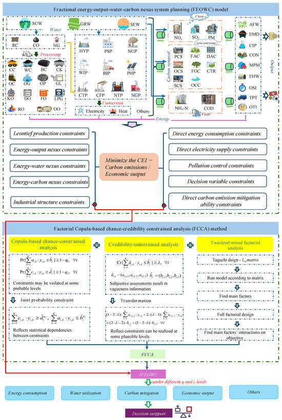
Figure 1. Development of the IFEOWC model.

3. Case Study

3.1. Study Area

Fujian is an important economic province, which is located in the southeast coastal area. According to the Fujian Energy Development Plan (2021–2025), improving tertiary industry development and enhancing low-carbon energy supply are significant actions to help maintain economy growth and achieve carbon neutrality. Meanwhile, the interactions between sectoral economic output, energy consumption, and carbon emission are complex. In 2017, metal product manufacture contributed 3.38% to the provincial output, while it consumed 22.83% of energy and emitted 5.88% of carbon; agriculture contributed 6.88% to the provincial output, while it consumed 1.81% of energy and emitted 5.04% of carbon. An effective tool which can balance these components to help generate management policies is urgently needed; this leads to the problem of CEI minimization with a system optimization model.

3.2. Data Collection and Processing

Monetary input–output table provides information about economic parameters in Leontief production constraints and industrial structure constraints. The table is often published every 5 years, while the 2022 table has not been published. The latest table (e.g., 2017) is collected from National Bureau of Statistics [52]. According to Fujian provincial Statistical Bulletin, Fujian’s economic structure has remained relatively stable [53]. The 2017 table is an acceptable data source. The 42 sectors in the original tables are integrated according to the nine sectors in the EOWC model. Official reports, academic articles, and industrial standards are the data sources of energy, water, carbon, and pollutant-related parameters [54,55,56,57,58,59,60,61,62,63]. After processing, crisp, random, and fuzzy parameters can be recognized. The model is tested and debugged prior to its formal operation. Crisp parameters are those that seemingly do not significantly affect the objective function values. Random and fuzzy parameters are determined based on the sufficiency of data and the characteristics of variables. Table 1 shows values of some random parameters that are interconnected (by conducting correlation analysis), and their values are determined by joint and marginal cumulative probability distributions. There are Gaussian, Clayton, Frank, and Gumbel copulas that can be chosen. The best one is decided through analyzing their Akaike Information Guidelines (AIC) and Bayesian information criteria (BIC) values (lower is better). It is assumed that the confidence level is not lower than 0.80 (i.e., 1 − q_joint = 1 − 0.20) and higher than 0.99 (i.e., 1 − q_joint = 1 − 0.01). Some medium-confidence levels (i.e., 0.95, 0.90, and 0.85) are chosen for detecting other probable results. The parameters’ values under different acceptable joint and marginal probabilities can then be obtained. For example, when q_joint = 0.01, $q_{{\widehat{DCC}}_{k=1,t}}-q_{{\widehat{TDQ}}_{w=1,t}}=0.010-0.010$, the raw coal demand and available surface water for sector AFW are 0.15 × 10⁶ tce and 1.23 × 10⁶ m³ in 2030. Table 2 lists values of some fuzzy variables. The lower bound (a) and upper bound (c) are the most possible value and least possible value, which are determined based on previous data and future assessment; the core value (b) is the middle value of a and c. For example, indirect water utilization allowance of sector AFW in 2030 is (6.37, 6.88, 7.39) × 10⁶ m³. When λ = 0.60, the value would be 6.88 + (1 − 2λ) × (6.88 − 6.37) = 6.78 × 10⁶ m³.

Table 1. Examples of random variable values under several joint and marginal probabilities.

Sector	qjoint	Raw Coal Demand–Available Surface Water qjoint, qx − qy: 0.010, 0.010 − 0.010 0.100, 0.073 − 0.100 0.200, 0.198 − 0.163		Raw Coal Demand–Carbon Emissions Allowance qjoint, qx − qy: 0.010, 0.010 − 0.010 0.100, 0.064 − 0.057 0.200, 0.141 − 0.141		Available Surface Water–Carbon Emissions Allowance qjoint qx − qy: 0.010, 0.010 − 0.010 0.100, 0.063 − 0.058 0.200, 0.133 − 0.149		Available Surface Water–Electricity Demand qjoint, qx − qy: 0.010, 0.010 − 0.010 0.100, 0.073 − 0.100 0.200, 0.198 − 0.163		Electricity Demand–Maximum Final Use qjoint, qx − qy: 0.010, 0.010 − 0.010 0.100, 0.078 − 0.099 0.200, 0.200 − 0.091
		Year: 2030	Year: 2060	Year: 2030	Year: 2060	Year: 2030	Year: 2060	Year: 2030	Year: 2060	Year: 2030	Year: 2060
AFW	0.010	0.15 − 1.23	0.10 − 3.45	0.15 − 3.48	0.10 − 0	1.23 − 3.48	3.45 − 0	1.23 − 7.93	3.45 − 17.38	7.93 − 0.39	17.38 − 0.55
	0.100	0.14 − 1.35	0.09 − 3.80	0.14 − 3.74	0.095 − 0	1.33 − 3.72	3.72 − 0	1.33 − 7.22	3.74 − 15.83	7.31 − 0.43	16.03 − 0.59
	0.200	0.13 − 1.29	0.09 − 3.90	0.13 − 3.88	0.090 − 0	1.38 − 3.89	3.86 − 0	1.41 − 7.02	3.95 − 15.38	6.92 − 0.42	15.17 − 0.59
EMD	0.010	0.22 − 0.77	0.21 − 3.25	0.22 − 1.99	0.21 − 0	0.77 − 1.99	3.25 − 0	0.77 − 1.58	3.25 − 1.61	1.58 − 0.036	1.61 − 0.13
	0.100	0.20 − 0.85	0.19 − 3.58	0.20 − 2.14	0.19 − 0	0.83 − 2.13	3.50 − 0	0.84 − 1.44	3.52 − 1.46	1.45 − 0.039	1.48 − 0.15
	0.200	0.19 − 0.87	0.18 − 3.67	0.19 − 2.22	0.18 − 0	0.86 − 2.23	3.63 − 0	0.88 − 1.40	3.72 − 1.42	1.38 − 0.039	1.40 − 0.14
CIP	0.010	2.40 − 9.11	1.64 − 7.24	2.40 − 12.63	1.64 − 0	9.11 − 12.63	7.24 − 0	9.11 − 48.21	7.24 − 70.31	48.21 − 0.21	70.31 − 0.33
	0.100	2.19 − 10.03	1.49 − 7.98	2.21 − 13.58	1.50 − 0	9.82 − 13.51	7.81 − 0	9.88 − 43.89	7.86 − 64.02	44.44 − 0.23	64.82 − 0.36
	0.200	2.05 − 10.30	1.40 − 8.19	2.10 − 14.11	1.43 − 0	10.18 − 14.15	8.10 − 0	10.42 − 42.65	8.29 − 62.20	42.07 − 0.23	61.35 − 0.36
CON	0.010	0.015 − 1.80	0.01 − 3.88	0.015 − 4.09	0.01 − 0	1.80 − 4.09	3.88 − 0	1.80 − 8.77	3.88 − 18.39	8.77 − 2.80	18.39 − 4.14
	0.100	0.014 − 1.99	0.009 − 4.27	0.014 − 4.40	0.009 − 0	1.94 − 4.38	4.18 − 0	1.96 − 7.98	4.21 − 16.74	8.08 − 3.02	16.95 − 4.47
	0.200	0.013 − 2.04	0.008 − 4.39	0.013 − 4.57	0.009 − 0	2.02 − 4.59	4.34 − 0	2.06 − 7.76	4.44 − 16.27	7.65 − 3.01	16.04 − 4.45
MPM	0.010	1.40 − 144.46	1.11 − 94.23	1.40 − 22.82	1.11 − 0	144.46 − 22.82	94.23 − 0	144.46 − 46.24	94.23 − 59.71	46.24 − 0.17	59.71 − 0.27
	0.100	1.28 − 159.14	1.02 − 103.81	1.29 − 24.55	1.02 − 0	155.73 − 24.43	101.58 − 0	156.74 − 42.10	102.24 − 54.37	42.63 − 0.19	55.05 − 0.29
	0.200	1.19 − 163.38	0.95 − 106.57	1.22 − 25.50	0.97 − 0	161.53 − 25.57	105.36 − 0	165.27 − 40.91	107.80 − 52.83	40.35 − 0.19	52.11 − 0.29
EHW	0.010	12.98 − 11.65	7.99 − 5.57	12.98 − 60.44	7.99 − 0	11.65 − 60.44	5.57 − 0	11.65 − 34.71	5.57 − 39.30	34.71 − 0.22	39.30 − 0.27
	0.100	11.86 − 12.84	7.30 − 6.13	11.94 − 65.01	7.35 − 0	12.56 − 64.69	6.00 − 0	12.64 − 31.60	6.04 − 35.78	32.00 − 0.24	36.23 − 0.29
	0.200	11.08 − 13.18	6.82 − 6.29	11.37 − 67.53	7.00 − 0	13.03 − 67.73	6.22 − 0	13.33 − 30.71	6.37 − 34.77	30.29 − 0.24	34.29 − 0.29
OSI	0.010	2.29 − 31.82	1.19 − 23.53	2.29 − 12.18	1.19 − 0	31.82 − 12.18	23.53 − 0	31.82 − 92.12	23.53 − 119.23	92.12 − 4.34	119.23 − 6.42
	0.100	2.09 − 35.05	1.08 − 25.92	2.11 − 13.10	1.09 − 0	34.30 − 13.04	25.37 − 0	34.52 − 83.88	25.53 − 108.56	84.93 − 4.69	109.92 − 6.93
	0.200	1.95 − 35.99	1.01 − 26.62	2.00 − 13.61	1.04 − 0	35.58 − 13.65	26.31 − 0	36.40 − 81.50	26.92 − 105.48	80.39 − 4.67	104.04 − 6.91
TPT	0.010	0.013 − 6.04	0.005 − 6.08	0.013 − 18.06	0.005 − 0	6.04 − 18.06	6.08 − 0	6.04 − 10.27	6.08 − 19.66	10.27 − 0.51	19.66 − 0.99
	0.100	0.012 − 6.65	0.005 − 6.70	0.012 − 19.43	0.005 − 0	6.51 − 19.33	6.56 − 0	6.55 − 9.35	6.60 − 17.90	9.47 − 0.55	18.12 − 1.07
	0.200	0.011 − 6.83	0.005 − 6.88	0.011 − 20.18	0.005 − 0	6.75 − 20.24	6.80 − 0	6.91 − 9.09	6.96 − 17.39	8.96 − 0.55	17.15 − 1.06
OTI	0.010	0.06 − 1.05	0.035 − 3.38	0.06 − 2.77	0.035 − 0	1.05 − 2.77	3.38 − 0	1.05 − 55.15	3.38 − 76.14	55.15 − 3.74	76.14 − 7.24
	0.100	0.055 − 1.16	0.032 − 3.72	0.055 − 2.98	0.032 − 0	1.13 − 2.97	3.64 − 0	1.14 − 50.22	3.66 − 69.32	50.85 − 4.04	70.19 − 7.82
	0.200	0.051 − 1.19	0.030 − 3.82	0.052 − 3.10	0.031 − 0	1.17 − 3.11	3.77 − 0	1.20 − 48.79	3.86 − 67.36	48.13 − 4.02	66.44 − 7.79

Note: Units for raw coal, water, carbon, electricity, and final use are 10⁶ tce, 10⁶ m³, 10⁶ t, 10⁹ kWh, and 10¹² RMB¥. This table only presents partial data due to space limitation.

Table 2. Examples of fuzzy variable values under several credibility degrees.

Parameter	Credibility	Year	AFW	EMD	CIP	CON	MPM	EHW	OSI	TPT	OTI
Indirect water utilization allowance (unit: 106 m3)	λ = 0.6	2030	6.78	2.45	38.76	11.09	184.88	461.14	54.15	53.04	4.79
		2060	6.20	2.50	32.46	8.58	153.66	306.35	47.27	38.48	4.89
	λ = 0.8	2030	6.58	2.37	37.59	10.76	179.32	447.27	52.52	51.44	4.65
		2060	6.02	2.43	31.48	8.33	149.03	297.13	45.85	37.32	4.74
	λ = 1.0	2030	6.37	2.30	36.43	10.42	173.76	433.40	50.89	49.85	4.51
		2060	5.83	2.35	30.50	8.07	144.41	287.92	44.42	36.17	4.60
Indirect carbon emissions allowance (unit: 106 t)	λ = 0.6	2030	20.68	2.08	5.97	298.83	2.98	2.43	409.45	36.05	162.78
		2060	8.52	2.62	0.02	224.20	7.54	40.17	312.94	39.58	159.71
	λ = 0.8	2030	20.05	2.01	5.79	289.84	2.89	2.36	397.13	34.96	157.89
		2060	8.27	2.54	0.02	217.45	7.31	38.96	303.52	38.39	154.91
	λ = 1.0	2030	19.43	1.95	5.61	280.86	2.80	2.29	384.82	33.88	152.99
		2060	8.01	2.46	0.02	210.71	7.08	37.75	294.11	37.20	150.10
Maximum carbon capture and storage ability (unit: 106 t)	λ = 0.6	2030	0	0.29	1.87	0.61	3.39	8.97	1.81	0	0
		2060	0	5.02	11.83	6.93	21.51	20.44	11.07	0	0
	λ = 0.8	2030	0	0.29	1.82	0.59	3.29	8.70	1.75	0	0
		2060	0	4.87	11.48	6.72	20.86	19.82	10.73	0	0
	λ = 1.0	2030	0	0.28	1.76	0.57	3.18	8.43	1.70	0	0
		2060	0	4.72	11.12	6.51	20.21	19.21	10.40	0	0
Maximum forest carbon sink ability (unit: 106 t)	λ = 0.6	2030	0.27	0.17	1.08	0.35	1.95	5.16	1.04	1.42	0.22
		2060	3.37	2.24	5.28	3.09	9.60	9.13	4.94	9.64	2.42
	λ = 0.8	2030	0.26	0.16	1.04	0.34	1.88	4.99	1.01	1.38	0.21
		2060	3.26	2.17	5.11	2.99	9.28	8.82	4.78	9.32	2.34
	λ = 1.0	2030	0.26	0.16	1.01	0.33	1.82	4.81	0.97	1.33	0.20
		2060	3.15	2.09	4.93	2.89	8.96	8.51	4.61	8.99	2.26
Carbon quota investment (unit: 109 CNY)	λ = 0.6	2030	0.049	0.028	0.179	0.058	0.323	0.855	0.172	0.256	0.039
		2060	0	0	0	0	0	0	0	0	0
	λ = 0.8	2030	0.048	0.027	0.173	0.056	0.313	0.830	0.167	0.248	0.038
		2060	0	0	0	0	0	0	0	0	0
	λ = 1.0	2030	0.046	0.026	0.168	0.054	0.304	0.804	0.162	0.240	0.037
		2060	0	0	0	0	0	0	0	0	0

3.3. Scenario Design

In the IFEOWC model, based on data processing, it is summarized that there are five kinds of random parameters: energy demand (${\widehat{DCC}}_{k,t}$, ${\widehat{DCR}}_{k,t}$, ${\widehat{DOC}}_{k,t}$, ${\widehat{DOO}}_{k,t}$, ${\widehat{ARC}}_{k,t}$, ${\widehat{AHC}}_{k,t}$ and ${\widehat{AOC}}_{k,t}$), available water (${\widehat{TDQ}}_{w,t}$), carbon emission allowance (${\widehat{DEA}}_{k,t}$), electricity demand (${\widehat{EFD}}_{k,t}$ and ${\widehat{RES}}_t$), and maximum final use (${\widehat{uf}}_{k,t}$). Ten groups of potential copula-based chance constraints are deigned based on combination: C(5, 2) = 5 * 4/2 = 10, with each group having five joint probabilities (q_joint = 0.01, 0.05, 0.10, 0.15, and 0.20). When considering one correlation (e.g., energy demand–available water, energy demand–carbon emission allowance, etc.), the other three types of parameters correspond to the values under marginal probability of 0.01. Thus, there are 50 chance-constrained scenarios. Parameters related to abilities such as ${\widetilde{TIME}}_{j,t}$, ${\widetilde{UPE}}_{j,t}$, ${\widetilde{LPE}}_{j,t}$, ${\widetilde{MSS}}_{k,t}$, ${\widetilde{IVC}}_{k,t}$, ${\widetilde{ZFP}}_t$, ${\widetilde{MIS}}_{k,t}$, ${\widetilde{MCS}}_{k,t}$, ${\widetilde{MUC}}_t$, ${\widetilde{MAC}}_t$, ${\widetilde{MUI}}_{u,t}$, ${\widetilde{MSI}}_{k,u,t}$, as well as allowances such as ${\widetilde{TIW}}_{k,t}$, ${\widetilde{TCA}}_{k,t}$, ${\widetilde{NEA}}_{k,t}$, ${\widetilde{NEC}}_{k,t}$ ${\widetilde{SEA}}_{k,t}$, ${\widetilde{NEN}}_{k,t}$, and ${\widetilde{PEN}}_{k,t}$ are featured with vagueness, and corresponding credibility constraints are assumed to be satisfied under five credibility degrees (λ = 0.5, 0.6, 0.7, 0.8, 0.9, and 1.0). All fuzzy parameters share identical λ levels, leading to five credibility-constrained scenarios. Overall, the multiple uncertainties are quantified and divided into 250 scenarios. Appendix B presents the scenario design framework. Solutions of the IFEOWC model are listed in Appendix C.

4. Results and Discussion

4.1. Carbon Emissions Intensity

Figure 2 shows the system CEI under all scenarios, which fluctuates in the range of 45.05 g/CNY under S5 (i.e., Scenario 5) to 47.67 g/CNY under S121. This implies that the random variable combinations, q_joint, and λ have effects on the CEI. For example, when q_joint = 0.01, λ = 0.6, the CEI corresponds to energy demand-available water (S1) and energy demand-carbon emission allowance (S26) would both approximately be 47.07 g/CNY; when considering energy demand–maximum final use, λ = 0.7, the CEI would be 47.14 g/CNY under q_joint = 0.01 (S81) and 46.30 g/CNY under q_joint = 0.20 (S85), respectively; when q_joint = 0.10, considering available water–electricity demand, the CEI would be 45.99 g/CNY under λ = 0.6 (S128) and 46.71 g/CNY under λ = 1.0 (S148). It can be found that (a) the effects are q_joint > combinations > λ; (b) the CEI would be lower under the higher q_joint levels and be higher under the higher λ levels; (c) energy demand–available water has greater impacts on the CEI than other combinations. Under conditions of low energy demand, high water availability, and high fuzzy parameter values, the CEI would reach its minimum value. Figure 3 presents the varied annual energy consumption, economic output, water utilization, and carbon emissions values under all scenarios. Over the 36 years, the total values would be 17.23 × 10⁹ tce to 18.84 × 10⁹ tce (energy), 729.70 × 10¹² CNY to 802.70 × 10¹² CNY (output), 29.30 × 10⁹ m³ to 32.01 × 10⁹ m³ (water), and 26.71 × 10⁹ t to 28.94 × 10⁹ t (carbon). Averagely, during 2025–2060, annual values would increase or decrease from 415.97 × 10⁶ tce to 503.46 × 10⁶ tce (energy), 12.61 × 10¹² CNY to 25.43 × 10¹² CNY (output), 824.78 × 10⁶ m³ to 671.98 × 10⁶ m³ (water), and decrease from 829.65 × 10⁶ t to 613.58 × 10⁶ t (carbon). It is indicated that the model can provide cost-effective, water-saving, and carbon-mitigation planning solutions to support the increased energy consumption.

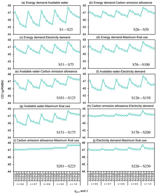
Figure 2. Total CEI under all scenarios.

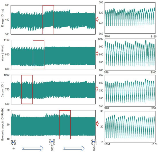
Figure 3. Total energy consumption, economic output, water utilization, and carbon emission values under all scenarios.

4.2. Energy Consumption

To analyze detailed results, eight typical scenarios (S5, S26, S55, S100, S105, S121, S150, S155) were selected based on random variable combinations and CEI variations. For instance, for energy demand–available water, the system would exhibit its minimum CEI under scenario S5 and maximum under S26. In Figure 4, it is shown that the total direct energy consumption values would vary with the changed scenarios, ranging from 7020.77 × 10⁶ tce to 7873.03 × 10⁶ tce over the 36 years. Such changes are mainly associated with combinations of random energy demand, electricity demand, and available water. On average, coal, natural gas, and oil products would account for 31.14%, 15.38%, and 29.65% of the total amount. The annual total amount of direct energy consumption would increase from about 182.22 × 10⁶ tce in 2025 to 217.90 × 10⁶ tce in 2060, due to the increment of energy demand. The shares of fossil fuels would be 79.57% in 2025 to 72.99% in 2060, relating to the higher energy demand and more strict carbon emission allowance. It is revealed that fossil fuels would still play vital roles in the energy consumption structure of Fujian. Policymakers should avoid abruptly closing coal product factories in Fujian.

During 2025–2060, the major sectors of consuming coal products would be EHW (about 45.77%) and MPM (about 43.60%); the main sectors of consuming natural gas products would be OSI (about 23.62%), MPM (about 10.37%) and TPT (about 10.13%); the great sectors of consuming oil products would be TPT (about 47.68%) and CIP (about 22.56%). In particular, the energy consumption of EHW would significantly decline because of the development of low-carbon energy conversion technologies (coal consumption would decrease by about 16.00%). For other sectors, in addition to traditional energy sources, electricity consumption would progressively increase. It is indicated that policymakers should highly promote electrification levels in Fujian, as well as supervise and urge these sectors to implement additional mitigation measures.

Figure 5 describes electricity structures under selected scenarios. Under each scenario, the proportions of fossil fuel electricity generation and low-carbon energy conversion would decrease and increase, respectively. For example, under S121, the proportion of CFP would drop from 45.67% in 2025 to 5.58% in 2060, while WIP and PHP would increase from 7.87% and 2.77 in 2025 to 22.63% and 14.88% in 2060. This means that low-carbon energy conversion capacities should be expanded from 52.18 × 10⁶ KW to 153.79 × 10⁶ KW (e.g., 26.60% for WIP, 24.05% for PHP, 21.08% for NUP) on average. Amid surging electrification level, CFP should be gradually phased out to meet emission allowance. Concurrently, WIP, PHP, and NUP should be prioritized as core alternatives, given their superior scalability and carbon neutrality.

Figure 4. Direct energy consumption values under selected scenarios.

Figure 5. Electricity structures under selected scenarios.

Figure 6 describes the indirect energy consumption values under each scenario. The annual total indirect energy consumption would show a tendency of first rising and then falling, reaching a peak in 2045. For instance, under S121, total indirect energy would rise from 237.31 × 10⁶ tce in 2025 to 324.11 × 10⁶ tce in 2045, and then would fall to 288.19 × 10⁶ tce in 2060. Over the 36 years, the major sectors of consuming energy would be OSI, TPT, and OTI, occupying about 16.98%, 19.09%, and 16.39% of the total amount. OSI would receive about 55.27% of energy from CON (e.g., raw materials for constructing factories, making glasses, etc.); TPT would receive about 71.54% of energy from CON (e.g., raw materials for building roads, bridges, etc.); OTI would receive 41.95% and 21.91% of energy from OSI (e.g., furniture, paper printing, etc.) and EHW (e.g., electricity) for supporting services. The important commodity transitions (i.e., CON→OSI, CON→TPT, and CON→OTI←EHW) reveal that OSI, TPT, and OTI are the great driving sectors that result in the high direct energy consumption. Policymakers can pay more attention to these sectors’ transactions when considering whether to reduce or increase direct energy consumption.

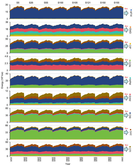
Figure 6. Indirect energy consumption values under selected scenarios.

4.3. Water Utilization

In Figure 7, the total direct water utilization would fluctuate between 18.92 × 10⁹ m³ and 20.45 × 10⁹ m³ over the 36 years under selected scenarios. These changes are related to the varied energy supply chain operations and carbon emission mitigation abilities. On average, the total utilization amount would increase from 517.41 × 10⁶ m³ in 2025 to 612.86 × 10⁶ m³ in 2042, and then decline to 451.44 × 10⁶ m³ in 2060, due to electricity substitution (e.g., WIP and PHP correspond to low water utilization efficiency) and technology upgrade (lead to high water utilization efficiency). The SUW, GRW, and SEW utilization would annually occupy about 36.57%, 9.37%, and 54.75%. MPM and OSI would be the major SUW (about 83.30%) and GRW (about 45.51%) users; EHW would be the main SEW (about 91.14%) user. This is because MPM, OSI, and EHW are the major energy consumers; thus, large amounts of water are needed to cooling machines for maintaining their normal operations. Results also discover that water for energy consumption and carbon emission mitigation would be approximately 99.32% and 0.68% (91.00%% for CCS, 9.00% for CSI) in 2025, 85.77% and 14.23% in 2060 (90.41% for CCS, 9.59% for CSI). It is implied that CCS and CSI would accelerate water shortage. Policymakers should ensure adequate water allocation for the implementation of CCS and CSI technologies.

In Figure 8, the tendency of annual indirect water utilization would align with the annual indirect energy consumption, while it would reach a peak in 2042. For instance, under S105, the total indirect water use would increase from 303.88 × 10⁶ m³ in 2025 to 356.54 × 10⁶ m³ in 2042, and then decrease to 226.98 × 10⁶ m³ in 2060. This is mainly decided by the indirect energy consumption and water utilization coefficient. Over the 36 years, the major sectors of consuming water would be EMD, OTI, and OSI, occupying about 31.23%, 26.09%, and 13.95% of the total amount. EMD would receive about 49.05% and 44.94% of water from EHW (e.g., electricity) and MPM (e.g., steel, machinery parts, etc.); OTI would receive about 79.05% of water from EHW (e.g., electricity); OSI would receive 46.45% and 35.72% of water from MPM (e.g., precision parts, conductive materials, etc.) and EHW (e.g., electricity) for supporting services. The commodity transitions (i.e., EHW→EMD←MPM, EHW→OTI, and MPM→OSI←EHW) reveal that EMD, OTI, and OSI are the driving sectors that lead to the high direct water utilization. Policymakers can regulate the direct water utilization through overseeing the inter-sectoral product transactions.

Figure 7. Direct water utilization values under selected scenarios.

Figure 8. Indirect water utilization values under selected scenarios.

4.4. Carbon Emissions

In Figure 9, it is shown that the total direct carbon emission would vary with the changed scenarios over the 36 years (i.e., from 7002. 61 × 10⁶ t to 81,421.93 × 10⁶ t) because of the changed energy consumption structure. The annual total amount would show a decreasing trend due to the low-carbon energy transition, averaging from 241.89 × 10⁶ t in 2025 to 175.72 × 10⁶ t in 2060. Through conducting carbon emission mitigation measures, final carbon emission (FIE) would approach a peak of 190.34 × 10⁶ t in 2026, and decrease to zero (i.e., carbon neutrality) in 2058. In the early planning years, CTR would be the most important measure due to the technologies of CCS and DCA, as well as the market of CSI, which is under developing. For example, in 2025–2040, the total amount of emission mitigation by CTR would be about 656.94 × 10⁶ t. The proportions of CCS, CSI, and DAC in emission mitigation would be 1.24%, 1.14%, and 0 in 2025, and increase to 34.88%, 42.13%, and 22.98% in 2060. For CCS, the abilities would be SCS > PCS > OCS; for CSI, the abilities would be OCC > FAC > FOC. Since CCS is a type of technology that captures carbon in the production plants, it is not suitable for non-point industry (e.g., AFW) or services-oriented industry (e.g., TPT and OTI). Thus, CCS is only conducted in the other six sectors. These results propose viable end removal solutions for carbon emission mitigation, thereby ensuring a low FIE. Along with carbon emission mitigation, pollution control can also not be neglected. Figure 10 shows that direct pollutant emissions/discharges would show obvious downward trends. It is implied that the changes in energy consumption structure and improvement treatment technologies could significantly reduce hazard martials in the environment.

In Figure 11, results show that the total indirect carbon emission would increase before 2033, and then continuously decline. For instance, under S121, the total amount would increase from 598.81 × 10⁶ t in 2025 to 633.46 × 10⁶ t in 2033 and then decrease to 439.40 × 10⁶ t in 2060. Annually, the great sectors of receiving carbon would be TPT (19.06%), OSI (16.88%), OTI (16.32%), and CIP (14.55%). TPT received 71.54% and 14.46% from CON and OSI; OSI received 55.27% and 16.40% from CON and OTI; OTI received 41.95% and 21.91% from OSI and EHW; CIP received 48.48% and 26.58% from OSI and CON. Commodity transitions among these sectors cannot be prohibited; thus, sectoral emissions are decided by the amount and structure of energy consumption, as well as carbon emission coefficient. Policies to change structure and decrease coefficient are needed to directly mitigate carbon emissions.

Figure 9. Direct carbon emissions values under selected scenarios.

Figure 10. Direct pollutant emissions/discharges under selected scenarios.

Figure 11. Indirect carbon emissions values under selected scenarios.

4.5. Economic Growth

Direct and indirect material flows (i.e., energy, water, and carbon) are highly related to final and intermediate uses (shown in Figure 12). Under the selected scenarios, the total sectoral use would annually increase with a rate of about 1.95% to 2.18%, and the ratios of final use would be about 68.23% to 71.46% in each year. It is implied that Fujian’s production activities would maintain steady economic growth. The sectoral use structure would be 1.93% (primary industry, i.e., AFW), 68.66% (secondary industry), 30.56% (tertiary industry, i.e., OTI and TPT) in 2025, and become 1.93%, 59.13%, 38.93% in 2060, respectively. OSI, OTI, and CON would dominate the total sectoral use, annually occupying 44.56%, 26.65%, and 16.51%; meanwhile, their final uses would contribute more than 98% of their total sectoral uses. This means that end-users’ demands are the greatest driving forces to the three sectors’ development. For other sectors, in addition to final uses, OSI and OTI would purchase large amounts of raw materials from them, leading to intensive transactions. It is indicated that OSI and OTI are pulling forces to push the developments of AFW, EMD, CIP, MPM, EHW, and TPT. Policymakers should implement supportive policies to foster the advancement of OSI and OTI.

4.6. Policy Implications

Policy implemented under S150 is identified as the most suitable one (i.e., available water–electricity demand, λ = 1, and q_joint = 0.20), since there is a balanced outcome is attainable here: carbon neutrality, high economic development, as well as restrained water utilization and energy consumption. Figure 13 and Figure 14 present the energy, output, water, and carbon flows in 2030 and 2060. Corresponding to the results, main policy implications are summarized as follows:

(1)

The adoption of advanced technologies for green low-carbon fossil fuel production is critical, given planned consumption would surge to 185.72 × 10⁶ tce by 2060.

(2)

The investment of low-carbon energy conversion capacities for green low-carbon electricity generation, e.g., WIP, PHP, and NUP would expand to 40.12 GW, 36.35 GW, and 31.78 GW by 2060;

(3)

The conduction of end-removal actions for reducing carbon in the air is essential, the contributions would plan to be CTR 18.73%, CCS 6.64%, CSI 3.14%, and DAC 0.27% in 2035, and CSI 40.40%, CCS 35.82%, and DAC 23.78% in 2060;

(4)

The strategic advancement of key sectors (e.g., CON, OSI and OTI) is significant to obtain great total economic outputs;

(5)

The reduction in freshwater allocation to the system is helpful for relieving water shortage, e.g., decreasing to 362.96 × 10⁶ m³ in 2030, and to 254.26 × 10⁶ m³ in 2060;

(6)

The seawater extraction volume should maintain at a stable level, e.g., 258.34 × 10⁶ m³ 2030 and 248.44 × 10⁶ m³ in 2060.

Figure 12. Intermediate use and final use values under selected scenarios.

Figure 13. Energy, output, water, and carbon flows in 2030 under S150.

Figure 14. Energy, output, water, and carbon flows in 2060 under S150.

4.7. Identifying Key Factors

Figure 15 provides the single and joint effects of key parameters on CEI variations. First, 15 potential key parameters are chosen and divided into two-levels (L for low value, H for high value). Through conducting Taguchi design, contribution rate of each single parameter affecting CEI variation are obtained εe (48.32%) > we (13.45%) > TGS (10.92%) > DOO (9.03%) > DCR (7.84%) > DCC (6.73%) > other parameters. It is also shown that the joint effect of two parameters is smaller than the single effect of one parameter. The joint effects of εe * we > TGS * DCC > DOO * DCC are more obvious than other combinations. It is indicated that studies need to be focused on reducing εe and we. The embodied energy consumption coefficient (εe) is calculated by dividing standard direct energy consumption into (final use minus intermediate use). Decreasing direct energy consumption (standard value) and increasing final use are helpful for reducing εe. It is found that the decoupling of energy consumption-final use is important. Introducing other cooling technologies (e.g., air cooling) to replace water cooling technology may be beneficial to reduce we.

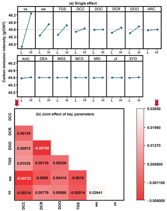
Figure 15. Single and joint effects of key parameters on CEI variations.

4.8. Comparison with Previous Studies

The comparison between the previous studies and our own results is analyzed. Several studies within the same topic, e.g., low-carbon emission energy system optimization, were published. Chen et al. (2023) developed a low-carbon electric power system optimization model in Canada; the results showed that renewable energy (i.e., wind and solar) would contribute to about 13% of the total national electricity generation by 2050 [64]. Zhen et al. (2024) proposed a renewable energy-based integrated energy system (under carbon trading mechanism) for communities, where energy saving, cost saving, and emission reduction planning schemes were obtained [65]. Wang et al. (2025) developed a low-carbon energy systems optimization in Nova Scotia (Canada); results indicated that the proportions of renewable energy and imported electricity on total energy consumption would highly increase [66]. Chen et al. (2025) proposed an energy-water–carbon system planning model in China; results showed that the system would reduce carbon emissions by 16.23%, air pollutant emissions by 19.31%, water consumption by 30.96%, and increase economic benefits by 10.97% [67]. These results align with the observed trend in this study’s findings, while random variable correlations, diverse mitigation measures, and Leontief production restrictions are neglected.

5. Conclusions

This study proposes an inexact fractional energy–output–water–carbon nexus system planning (IFEOWC) model to detect low-carbon development pathways considering the four elements’ nexus relationships under randomness and fuzziness information. The objective is to minimize the carbon emission intensity (CEI), subjecting to the Leontief production, energy–output nexus, energy–water nexus, energy–carbon nexus, direct energy consumption, direct electricity supply, direct carbon emission, direct water utilization, industrial structure, pollution control constraints, etc. The model is applied in Fujian province, China. Ten groups of potential copula-based chance-constraints with five joint probabilities (q_joint), and five credibility degrees (λ) for each credibility-constraint are considered, resulting in 250 scenarios. Optimal policies relating to direct (by production processes) and indirect (by-products/services transactions) energy consumption, economic growth, water utilization, and carbon emissions are obtained. Some major findings of the case study are summarized:

(1) The effects of uncertainties on the CEI are q_joint > combinations (especially energy demand-available water) > λ, and the CEI would fluctuate between 45.05 g/CNY and 47.67 g/CNY; (2) the annual shares of fossil fuels would maintain at a high level ([72.99, 79.58] %); low-carbon energy conversion capacities such as WIP, PHP, and NUP would expand to [39.49, 42.01] GW, [33.48, 38.76] GW, [31.23, 33.23] GW for fulfilling the increased energy demand, the limited water resources, and the restricted carbon emission; (3) SEW would always be the main direct water source (annually occupying [51.15, 58.34]%); (4) OTI, OSI, CON would be the major final demand supply sectors (annually occupying [87.79, 88.42]%); (5) approximately, the ability to mitigate direct carbon emission would be CTR (19.11%) > FOC (1.07%) > PCS (0.84%) > SCS (0.35%) > others (0.12%) in 2025, and gradually become DAC (22.98%) > FOC (22.11%) > SCS (15.73%) > PCS (13.01%) > OCC (12.90%) > FAC (7.12%) > OCS (6.14%) in 2060.

The developed model can be utilized by decision makers when formulating provincial development plans (e.g., Special Planning for Energy Development, National economic development plan, etc.). The optimal regional policies can also provide ecological and low-carbon socio-economic development directions to larger territories. Such policies are often enforced under the oversight of competent authorities.

Several limitations require targeted interventions in subsequent research phases. First, alternative uncertainty analysis approaches, such as interval parameter programming and two-stage programming can be introduced into the system. They can convert deterministic parameters into bounded intervals to quantify uncertainty and decompose decision-making into sequential phases (initial target and recourse decisions) to systematically mitigate risk exposure. Second, prediction models can be employed to forecast key parameter values (e.g., electricity demand), thereby enhancing the accuracy of system objective values. Third, additional carbon emission mitigation measures can be explored to identify diverse pathways for reduction.

References

- Duan, H.Y.; Sun, X.H.; Song, J.N.; Xing, J.H.; Yang, W. Peaking carbon emissions under a coupled socioeconomic-energy system: Evidence from typical developed countries. Resour. Conserv. Recycl. 2022, 187, 106641. [Google Scholar] [CrossRef]
- Energy Institute (EI). Statistical Review of World Energy 2024; Energy Institute: London, UK, 2024. [Google Scholar]
- Liu, J.; Zhao, S.H.; Li, Y.P.; Sun, Z.M. Development of an interval double-stochastic carbon-neutral electric power system planning model: A case study of Fujian province, China. J. Clean. Prod. 2023, 425, 138877. [Google Scholar] [CrossRef]
- Yu, Z.; Khan, S.A.R.; Ponce, P.; Jabbour, A.B.L.D.S.; Jabbour, C.J.C. Factors affecting carbon emissions in emerging economies in the context of a green recovery: Implications for sustainable development goals. Technol. Forecast. Soc. Change 2022, 176, 121417. [Google Scholar] [CrossRef]
- Cao, R.; Huang, G.H.; Chen, J.P.; Li, Y.P. A fractional multi-stage simulation-optimization energy model for carbon emissions management of urban agglomeration. Sci. Total Environ. 2021, 774, 144963. [Google Scholar] [CrossRef]
- Liang, M.S.; Huang, G.H.; Chen, J.P.; Li, Y.P. Energy-water-carbon nexus system planning: A case study of Yangtze River Delta urban agglomeration, China. Appl. Energy 2022, 308, 118144. [Google Scholar] [CrossRef]
- Lin, X.J.; Huang, G.H.; Zhou, X.; Zhai, Y.Y. An inexact fractional multi-stage programming (IFMSP) method for planning renewable electric power system. Renew. Sustain. Energy Rev. 2023, 187, 113611. [Google Scholar] [CrossRef]
- Zheng, Y.L.; Huang, G.H.; Li, Y.P.; Chen, J.P.; Zhou, X.; Luo, B.; Fu, Y.P.; Lin, L.J.; Xu, Z.P.; Tang, W.C. An in deterministic fractional two-stage inter-regional energy system optimization model: A case study for the Province of Shanxi, China. J. Clean. Prod. 2024, 435, 140330. [Google Scholar] [CrossRef]
- Li, H.; Wang, J.; Lu, Z.; Zhang, Y.; Hou, G.; Xue, L. Process analysis-based industrial production modelling with uncertainty: A linear fractional programming for joint optimization of total carbon emissions and emission intensity. Appl. Energy 2025, 382, 125204. [Google Scholar] [CrossRef]
- Tabatabaie, S.M.H.; Murthy, G.S. Development of an input-output model for food-energy-water nexus in the pacific northwest, USA. Resour. Conserv. Recycl. 2021, 168, 105267. [Google Scholar] [CrossRef]
- He, P.; Ng, T.S.; Su, B. Energy-economic resilience with multi-region input-output linear programming models. Energy Econ. 2019, 84, 104569. [Google Scholar] [CrossRef]
- Zhou, X.; Gu, A. Impacts of household living consumption on energy use and carbon emissions in China based on the input-output model. Adv. Clim. Change Res. 2020, 11, 118–130. [Google Scholar] [CrossRef]
- Kang, J.D.; Ng, T.S.; Su, B.; Milovanoff, A. Electrifying light-duty passenger transport for CO2 emissions reduction: A stochastic-robust input-output linear programming model. Energy Econ. 2021, 104, 105623. [Google Scholar] [CrossRef]
- Kang, J.D.; Wu, Z.; Ng, T.; Su, B. A stochastic-robust optimization model for inter-regional power system planning. Eur. J. Oper. Res. 2023, 310, 1234–1248. [Google Scholar] [CrossRef]
- Zhang, Q.Q.; Jie, D.; Li, J.; Zhou, J. Carbon compensation cost in Jing-Jin-Ji region under the carbon neutrality goal: Considering emission responsibility and carbon abatement cost. J. Clean. Prod. 2024, 467, 142950. [Google Scholar] [CrossRef]
- Alyousif, M.; Belaid, F.; Almubarak, A.; Almulhim, T. Mapping Saudi Arabia’s low emissions transition path by 2060: An input-output analysis. Technol. Forecast. Soc. Change 2025, 211, 123920. [Google Scholar] [CrossRef]
- Tan, Q.; Liu, Y.; Ye, Q. The impact of clean development mechanism on energy-water-carbon nexus optimization in Hebei, China: A hierarchical model based discussion. J. Environ. Manag. 2020, 264, 110441. [Google Scholar] [CrossRef] [PubMed]
- Mehrjerdi, H.; Aljabery, A.A.M. Modeling and optimal planning of an energy-water-carbon nexus system for sustainable development of local communities. Adv. Sustain. Syst. 2021, 5, 2100024. [Google Scholar] [CrossRef]
- Liang, M.S.; Huang, G.H.; Chen, J.P.; Li, Y.P. Development of non-deterministic energy-water-carbon nexus planning model: A case study of Shanghai, China. Energy 2022, 246, 123300. [Google Scholar] [CrossRef]
- Yu, D.M.; Li, Z.M.; Fan, S.Y.; Sun, T.Y. Optimal management of an energy-water-carbon nexus employing carbon capturing and storing technology via downside risk constraint approach. J. Clean. Prod. 2023, 418, 138168. [Google Scholar] [CrossRef]
- Valencia-Díaz, A.; Toro, E.M.; Hincapié, R.A. Optimal planning and management of the energy-water-carbon nexus in hybrid AC/DC microgrids for sustainable development of remote communities. Appl. Energy 2025, 377, 124517. [Google Scholar] [CrossRef]
- Zhu, Y.; Chen, M.; Yang, Q.; Alshwaikh, M.J.M.; Zhou, H.; Li, J.; Liu, Z.; Zhao, H.; Zheng, C.; Bartocci, P.; et al. Life cycle water consumption for oxyfuel combustion power generation with carbon capture and storage. J. Clean. Prod. 2021, 281, 124419. [Google Scholar] [CrossRef]
- Rosa, L.; Sanchez, D.L.; Realmonte, G.; Baldocchi, D.; D’Odorico, P. The water footprint of carbon capture and storage technologies. Renew. Sustain. Energy Rev. 2021, 138, 110511. [Google Scholar] [CrossRef]
- Zhang, D.; Zuo, X.; Zang, C. Assessment of future potential carbon sequestration and water consumption in the construction area of the Three-North Shelterbelt Programme in China. Agric. For. Meteorol. 2021, 303, 108377. [Google Scholar] [CrossRef]
- Wu, H.; Guo, S.; Guo, P.; Shan, B.; Zhang, Y. Agricultural water and land resources allocation considering carbon sink/source and water scarcity/degradation footprint. Sci. Total Environ. 2022, 819, 152058. [Google Scholar] [CrossRef]
- Daneshvar, M.; Mohammadi-Ivatloo, B.; Asadi, S.; Anvari-Moghaddam, A.; Rasouli, M.; Gharehpetian, G.B. Chance-constrained models for transactive energy management of interconnected microgrid clusters. J. Clean. Prod. 2020, 271, 122177. [Google Scholar] [CrossRef]
- Li, H.W.; Li, Y.P.; Huang, G.H.; Gao, P.P. Identifying optimal land-use patterns using a copula-based interval stochastic programming model for urban agglomeration under uncertainty. Ecol. Eng. 2020, 142, 105616. [Google Scholar] [CrossRef]
- Wang, Y.M.; Zhu, G.C. A mixed integer fuzzy-interval credibility-constrained programming for booster optimization in water distribution system under uncertainty. J. Water Process Eng. 2022, 50, 103300. [Google Scholar] [CrossRef]
- Zhang, Y.; Yang, P. An inexact multi-objective mixed-integer nonlinear programming approach for water-soil-fertilizer management under uncertainty considering “footprint family-planetary boundary” assessment. J. Hydrol. 2023, 626, 129471. [Google Scholar] [CrossRef]
- Jankovic, A.; Chaudhary, G.; Goia, F. Designing the design of experiments (DOE)-An investigation on the influence of different factorial designs on the characterization of complex systems. Energy Build. 2021, 250, 111298. [Google Scholar] [CrossRef]
- Colette, D.A.; Martial, D.A.C.; Joseph, A.Y.; Benjamin, Y.K.; Patrick, D.A. Optimization of the compressive strength of used tire/cement phase composite concretes using a full factorial design. Constr. Build. Mater. 2023, 404, 133252. [Google Scholar] [CrossRef]
- Wang, G.Y.; Li, Y.P.; Liu, J.; Huang, G.H.; Chen, L.R.; Yang, Y.H.; Gao, P. A two-phase factorial input-output model for analyzing CO2-emission reduction pathway and strategy from multiple perspectives—A case study of Fujian province. Energy 2022, 248, 123615. [Google Scholar] [CrossRef]
- Leontief, W.W. Input-Output Economics, 2nd ed.; Oxford University Press: Oxford, UK, 1986. [Google Scholar]
- Kang, J.D.; Ng, T.S.; Su, B.; Yuan, R. Optimizing the Chinese electricity mix for CO2 emission reduction: An input-output linear programming model with endogenous capital. Environ. Sci. Technol. 2020, 54, 697–706. [Google Scholar] [CrossRef]
- Jirdehi, M.A.; Tabar, V.S. Multi-objective long-term expansion planning of electric vehicle infrastructures integrated with wind and solar units under the uncertain environment considering demand side management: A real test case. Sustain. Cities Soc. 2023, 96, 104632. [Google Scholar] [CrossRef]
- Nazloo, H.T.; Babazadeh, R.; Varmazyar, M. Optimal Configuration and Planning of Distributed Energy Systems Considering Renewable Energy Resources. J. Environ. Inform. 2024, 43, 50–64. [Google Scholar]
- Yu, L.; Zheng, S.; Gao, Q. Independent or collaborative management? Regional management strategy for ocean carbon sink trading based on game theory. Ocean Coast. Manag. 2023, 235, 106484. [Google Scholar] [CrossRef]
- Ke, S.; Zhang, Z.; Wang, Y. China’s forest carbon sinks and mitigation potential from carbon sequestration trading perspective. Ecol. Indic. 2023, 148, 110054. [Google Scholar] [CrossRef]
- Song, S.; Kong, M.; Su, M.; Ma, Y. Study on carbon sink of cropland and influencing factors: A multiscale analysis based on geographical weighted regression model. J. Clean. Prod. 2024, 447, 141455. [Google Scholar] [CrossRef]
- Sun, B.; Fan, B.; Wu, C.; Xie, J. Exploring incentive mechanisms for the CCUS project in China’s coal-fired power plants: An option-game approach. Energy 2024, 288, 129694. [Google Scholar] [CrossRef]
- Hu, Y.; Gani, R.; Sundmacher, K.; Zhou, T. Assessing the future impact of 12 direct air capture technologies. Chem. Eng. Sci. 2024, 298, 120423. [Google Scholar] [CrossRef]
- Li, J.; Zhang, Y.; Deng, Y.; Xu, D.; Tian, Y.; Xie, K. Water consumption and conservation assessment of the coal power industry in China. Sustain. Energy Technol. Assess. 2021, 47, 101464. [Google Scholar] [CrossRef]
- Wang, Y.; Lu, Y.; Xu, Y.; Zheng, L.; Fan, Y. A factorial inexact copula stochastic programming (FICSP) approach for water-energy- food nexus system management. Agric. Water Manag. 2023, 277, 108069. [Google Scholar] [CrossRef]
- Liu, Y.; Tan, J.; Wei, Z.; Zhu, Y.; Chang, S.; Li, Y.; Li, S.; Guo, Y. Analysis of Extreme Random Uncertainty in Energy and Environment Systems for Coal-Dependent City by a Copula-Based Interval Cost–Benefit Stochastic Approach. Sustainability 2024, 16, 745. [Google Scholar] [CrossRef]
- Kaytez, F. Evaluation of priority strategies for the expansion of installed wind power capacity in Turkey using a fuzzy analytic network process analysis. Renew. Energy 2022, 196, 1281–1293. [Google Scholar] [CrossRef]
- Zhang, C.; Yang, G.; Wang, C.; Huo, Z. Linking agricultural water-food-environment nexus with crop area planning: A fuzzy credibility-based multi-objective linear fractional programming approach. Agric. Water Manag. 2023, 277, 108135. [Google Scholar] [CrossRef]
- Huang, K.; Fang, Y.R. Parameter Uncertainty and Sensitivity Evaluation of Copula-Based Multivariate Hydroclimatic Risk Assessment. J. Environ. Inform. 2021, 38, 131–144. [Google Scholar] [CrossRef]
- Zhang, S.Q.; Li, Y.P.; Huang, G.H.; Ding, Y.K.; Yang, X. Developing a copula-based input-output method for analyzing energy-water nexus of Tajikistan. Energy 2023, 266, 126511. [Google Scholar] [CrossRef]
- Zhang, T.; Tan, Q.; Cai, Y.; Hu, K. A copula-based inexact model for managing agricultural water-energy-food nexus under differentiated composite risks and dual uncertainties. J. Clean. Prod. 2024, 434, 139707. [Google Scholar] [CrossRef]
- Liu, J.; Nie, S.; Shan, B.G.; Li, Y.P.; Huang, G.H.; Liu, Z.P. Development of an interval-credibility-chance constrained energy-water nexus system planning model-case study of Xiamen, China. Energy 2019, 181, 677–693. [Google Scholar] [CrossRef]
- Hwang, H.; Kim, S. Investigation on the effective factor calculation of electropolishing using full factorial design and mechanism model by microscopic analysis for super austenitic stainless steel. Surf. Interfaces 2023, 37, 102730. [Google Scholar] [CrossRef]
- National Bureau of Statistics (NBS). China Statistic Yearbook; China Statistics Press: Beijing, China, 2022.
- Fujian Statistics Bureau (FSB). Fujian Statistical Yearbook; China Statistics Press: Beijing, China, 2022.
- GB 20426-2006; Emission Standard for Pollutants from Coal Industry. Ministry of Ecology and Environment of the People’s Republic of China: Shanghai, Chian, 2006.
- GB 13223-2011; Emission Standard of Air Pollutants for Thermal Power Plants. Ministry of Ecology and Environment of the People’s Republic of China: Shanghai, Chian, 2011.
- GB 39728-2020; Emission Standard of Air Pollutants for Onshore Oil and Gas Exploitation and Production Industry. Ministry of Ecology and Environment of the People’s Republic of China: Shanghai, Chian, 2020.
- China Emission Accounts & Datasets (CAEDs). Latest Energy Inventories for China and its 30 Provinces and Cities. Compiled by Tsinghua University, China Emission Accounts & Datasets. 2021. Available online: https://www.ceads.net/data/province/energy_inventory/ (accessed on 15 October 2024).
- Jia, C.H.; Yan, P.; Liu, P.; Li, Z. Energy industrial water withdrawal under different energy development scenarios: A multi-regional approach and a case study of China. Renew. Sustain. Energy Rev. 2021, 135, 110224. [Google Scholar] [CrossRef]
- Fujian Provincial Department of Water Resources (FWR). Fujian Water Resources Bulletin; FWR: Fuzhou, China, 2022.
- Fujian Provincial Department of Ecology and Environment (FDE). Fujian Province Industrial Carbon Peak Implementation Plan. Guided by Ministry of Ecology and Environment of the People’s Republic of China; FDE: Fuzhou, China, 2023.
- DB35/T 772-2023; Norm of Water Intake of Industries. Fujian Province Market Supervision Administration: Fuzhou, China, 2023.
- Cao, X.; Liu, C.; Wu, M.X.; Li, Z.; Wang, Y.H.; Wen, Z.G. Heterogeneity and connection in the spatial-temporal evolution trend of China’s energy consumption at provincial level. Appl. Energy 2023, 336, 120842. [Google Scholar] [CrossRef]
- Dong, H.H.; Yang, J. Study on regional carbon quota allocation at provincial level in China from the perspective of carbon peak. J. Environ. Manag. 2024, 351, 119720. [Google Scholar] [CrossRef] [PubMed]
- Chen, L.; Huang, G.; Chen, J.; Luo, B. Development of a multi-regional factorial optimization model for supporting electric power system’s low-carbon transition—A case study of Canada. Resour. Conserv. Recycl. 2023, 194, 106995. [Google Scholar] [CrossRef]
- Zhen, J.; Liu, X.; Wu, C.; Ji, L.; Huang, G. Operation optimization and performance evaluation of photovoltaic-wind-hydrogen-based integrated energy system under carbon trading mechanism and uncertainty for urban communities. J. Clean. Prod. 2024, 476, 143688. [Google Scholar] [CrossRef]
- Wang, S.; Huang, G.; Zhou, X.; Tian, C. A dual-interval fractional energy systems optimization for Nova Scotia, Canada. Renew. Sustain. Energy Rev. 2025, 212, 115455. [Google Scholar] [CrossRef]
- Chen, Y.; Huang, G.; Liu, Y.; Luo, B.; Wang, S.; Li, Y.; LI, X. Energy-water-carbon system management in response to climate change in China under uncertainties (2026–2050). Resour. Conserv. Recycl. 2025, 212, 107957. [Google Scholar] [CrossRef]
Disclaimer/Publisher’s Note: The statements, opinions and data contained in all publications are solely those of the individual author(s) and contributor(s) and not of MDPI and/or the editor(s). MDPI and/or the editor(s) disclaim responsibility for any injury to people or property resulting from any ideas, methods, instructions or products referred to in the content. |
© 2025 by the authors. Licensee MDPI, Basel, Switzerland. This article is an open access article distributed under the terms and conditions of the Creative Commons Attribution (CC BY) license (https://creativecommons.org/licenses/by/4.0/).