Sustainable Local Employment Gains from Marcellus Shale Gas Extraction, or Modest and Temporary?

Abstract

Localized employment gains from new or expanded fossil fuel development commonly are cited by its proponents in response to sustainability-related concerns raised by local drilling area residents. This paper analyzes local employment effects in drilling areas within the Marcellus shale formation in the state of Pennsylvania, USA. The Marcellus shale formation was one of the early natural gas fracking boom development areas globally, so these local employment outcomes can inform future policy decisions on not-yet-developed shale gas formations worldwide. As long-term sustainable jobs are a key part of any locale’s sustainable development program, the magnitude and persistence of employment gains in the local drilling area is highly relevant. The existing research literature on employment effects from increased shale gas extraction is dominated by usage of panel estimation on annual data at the U.S. state/county level. The innovative contribution of this paper is its use of monthly data, sub-state local areas (67 counties within PA), and a parsimonious vector autoregression model (VAR) estimated separately for each of the 67 counties. The estimated VAR models are used to ascertain whether Marcellus shale drilling activity in PA led to actual county-level employment above forecasted based on data prior to the shale boom. Actual versus forecasted employment is compared from 2010–2019. Higher than forecasted employment findings were much more likely to occur in approximately the top quarter of drilling counties, with the observed gains being modest. Most importantly, however, any employment gains above forecast were short-lived, gone within four years in most counties. Given the modest and temporary local employment gains found and the many known potential damages to local residents and the environment from intensive drilling, it is questionable that the local areas in the Marcellus shale formation most intensively drilled benefited overall from the shale gas extraction. These findings are germane to ongoing current debates about expanding natural-gas-fired electricity generation, versus solar plus storage, to meet anticipated large rises in electricity demand from rapid data center development globally.

1. Introduction and Literature Review

1.1. Global Relevance of Marcellus Shale Outcomes

The widespread adoption of hydraulic fracturing (fracking) techniques used to extract oil and natural gas from shale formations has been an exceptionally transformative technology in the oil and gas industry. There now exists a large, and still growing, literature on the many pathways by which fracking impacts energy markets, economic growth, labor markets, environmental quality, health exposure risks, and issues arising from transient industry workers. This paper confines itself to an analysis of the local economic impact from natural gas fracking of the Marcellus shale formation conducted in the state of Pennsylvania in the United States. Proponents of its development, and other regions with fracking potential, frequently promote employment gains to the local drilling areas when any sustainability-related concerns are voiced about the drilling and extraction of natural gas. The practical significance of this paper’s findings is the ephemeral nature of any local drilling area employment gains above forecasted expectations. If the heavily drilled Marcellus shale area fails to generate sustainable increases in local employment for the local drilling areas, then this result should inform other policymakers, and citizens, in areas being pressured by industry advocates to initiate shale gas extraction.

While narrow in geographic focus, the study is relevant to the evolving circumstances related to the explosive growth in artificial intelligence (AI)-focused data centers and growing demand for natural-gas-generated electricity to help meet this growth. The International Energy Agency notes that a typical existing AI-focused data center consumes electricity equal to the usage of 100,000 households, that the largest ones under construction will raise that equivalency to 2,000,000 households, and it forecasts that natural gas usage will expand by 175 terawatt-hours to help meet growing data center power needs by 2030 [1]. Any expansion of natural gas fracking into new regions globally will have its proponents emphasizing the positive impact for workers in the new drilling regions. It will be informative to carefully analyze the local labor market impacts over time from the Marcellus shale formation in the state of Pennsylvania (PA) in the United States, as this region was one of the early natural gas fracking boom development areas globally.

Prior to 2009, Pennsylvania shale gas production was less than 0.1% of annual national shale gas production, but the drilling ramp-up in 2009 raised the state’s total to 2.1% that year and to 30.2% by 2015 [2]. Pennsylvania’s 4.6 trillion cubic feet of shale gas production in 2015 accounted for more than 95% of total natural gas production in the state [3]. To be sure, Marcellus shale gas production in Pennsylvania substantially altered natural gas markets in the United States. From 2007 to 2015, total U.S. natural gas production rose by a third, from 24.7 to 32.9 trillion cubic feet, and increased output from Pennsylvania accounted for 56.2% of the national rise in production over that period (EIA, 2023c [3]).

1.2. Industry Job Claims from Input–Output Modelling and Critiques

There are multiple plausible pathways by which the emergence of shale gas extraction in a region may have a positive impact on local area employment. Naturally, during the intensive drilling stage of development there will be jobs at both the drilling sites and for the area from businesses providing supporting services such as trucking of water and fracking liquids, piping, and other more general supplies. Additional employment can arise from the need to build out local area pipelines to connect the new production to the region’s pipeline distribution network. Local services related to housing, dining, and entertainment also may see rising demand. Over time, an intensively drilled area may develop the specific human capital in its labor force needed for the local area to become a specialized supplier of key materials and professional services for the industry. If the pace of local drilling activity fades over time, a common boom–bust outcome in mineral and energy extraction, then the employment boost from the intensive drilling may fade. A long-term employment gain after the drilling boom can arise if the boom period led to the development of industry-supporting businesses that are able to make sales to other regions or if the boom generated sufficient wealth that remained in the local area so that it raised the baseline employment level due to increasing demand for local services.

Optimism among Pennsylvania shale gas industry proponents about the job-generating potential for the state was boosted by two controversial studies conducted by academic researchers using the IMPLAN input–output model, but these studies were not subject to peer review. They estimated that the 2008 Marcellus-shale-related activity generated over 29,000 jobs in Pennsylvania [4], and their updated study claimed that more than 44,000 jobs were generated in 2009 by shale gas drilling in the state [5]. As also reviewed by Hoy and colleagues [6], these estimates soon were criticized heavily for the strong pro-industry assumptions used to generate the job growth forecasts. Kinnaman [7] was amongst the first peer-reviewed criticisms of these studies, calling attention to unrealistic assumptions regarding when and where households receiving royalty payments spend the money as well as the location, in state or out-of-state, of both suppliers to Pennsylvania drilling activity and households receiving royalty payments.

Kinnaman [7] and Hoy et al. [6] note that the job growth forecasts by the Considine group unrealistically assumed that 95% of industry spending went to workers and suppliers within Pennsylvania in 2008 and 2009, despite the fact that this drilling technology was new to the state and initially dependent upon considerable amounts of out-of-state labor and technical expertise. Perhaps even less credibly, the Considine studies assumed that all royalty and related production payments went to landowners in Pennsylvania, over USD 2 billion in 2008 alone, and all of the funds were spent in the year received. The former assumption is dubious given the stage of the industry’s development in Pennsylvania in 2008 and 2009. The latter assumption contradicts the many research findings that households save at least some portion of windfall income gains.

Hoy et al. [6] used detailed GIS data on well locations for two of the most drilling-intensive counties in Pennsylvania to conduct a large survey of households near active wells in order to more intensively sample households receiving natural gas lease and royalty payments. They found that landowners did not spend all received payments immediately, saving about 55% of leasing fees and 66% of royalty payments. Moreover, the types of purchases made differed from households’ standard consumption patterns, with a higher percentage of spending on consumer durables and motor vehicles. This spending will have a higher rate of leakage outside of the immediate county than average spending by households, which lowers the local employment multiplier from the natural gas payments to landowners. They also utilized survey data indicating that only 62.7% of Pennsylvania shale gas workers were state residents [8]. When these findings are incorporated into the IMPLAN model, the 2009 Pennsylvania job growth from Marcellus shale is estimated in the range of 23,385 to 23,884 jobs [6], which is well below the 44,098 estimate from Considine et al. [5].

For perspective, the 2009 Pennsylvania state total non-farm employment was 5.6 million, so the 2009 Marcellus employment estimate of 23,884 was only 0.4% of state non-farm employment that year. This relatively small contribution to total state employment, however, does not mean that there are not noticeable local employment impacts from Marcellus shale gas drilling in Pennsylvania for two reasons. First, the industry grew substantially in the state since 2009, so more recent employment effects may be larger. Also, the drilling activity is not uniformly distributed across the state. As discussed in later sections, the Marcellus shale drilling activity is relatively concentrated in less than ten of the state’s sixty-seven counties, none of which are intensively urban, so it is possible that the drilling activity has had discernable employment impacts for some counties more than others.

1.3. Estimates of Employment from Fracking Using Annual Panel Data Regression

In addition to using input–output models, there is a sizeable literature on the employment effects from shale oil and gas drilling that utilizes a variety of statistical techniques. Most of these studies utilize annual data at the U.S. state/county level. One of the early works was by Weber [9], who analyzed changes in county-level employment using annual data from 1999 to 2007 for 209 non-metro Colorado, Texas, and Wyoming counties, 61 of which were classified as drilling boom counties. Weber estimates that each million USD of natural gas produced in a county creates 2.35 jobs in the county. Weber [10] extended this work to analyze 362 non-metro counties in Arkansas, Louisiana, and Oklahoma using annual data from 1995 to 2010 and found that each natural-gas-related production job in a county led to more than one non-mining county job created. An analysis of 207 counties in six western states having oil and natural gas production by Haggerty and colleagues [11], however, using annual data for 1980 to 2011 found a negative impact from drilling activity upon the change over the period in real per capita income.

Weinstein [12] also uses annual data for 3060 counties in the contiguous U.S. states for 2001 to 2011 to estimate employment effects for drilling boom counties over that period and finds a county employment multiplier of only 1.3 total jobs per job generated in the oil and gas sector. Maniloff and Mastromonaco [13] again use annual data from 2005 and 2011 for 3018 non-urban counties to estimate the impact of shale oil and gas development changes on county employment and income. Nationally, they estimate 555,541 jobs created from 2005 to 2011 by increased shale oil and gas drilling, with Pennsylvania and Texas accounting for 299,876 and 169,536 jobs, respectively. Lee (2015) [14] focuses solely upon the 254 Texas counties using annual data from 2009 to 2014 and estimates that one additional newly drilled gas well in a county generates 15.6 jobs in the county. Feyrer et al. [15] estimate local economic impacts from fracking using annual data from 2004 to 2012 for 3018 counties. They find that each additional million dollars of oil or gas production generates 0.85 jobs at the county level and 2.13 jobs within a 100-mile radius of the well location. With the longer time frame of 1993 to 2013 and annual data for 1039 counties, Tsvetkova and Partridge [16] find that equal-sized shocks create more employment when the shocks are in the rest of the economy versus the oil and gas sector. When they confine their analysis to non-metro counties in the top 20 percent of energy sector expansion, the estimated impact from energy employment growth is 25.9 total new jobs if at the median county employment of 5876, an increase of 0.4%.

1.4. Estimates of Employment from Fracking Using Other Techniques

Munasib and Rickman [17] apply synthetic control analytic methods to various shale gas and oil boom counties. Their Marcellus shale analysis uses annual employment data from 20 different Pennsylvania counties, and they fail to find any statistically significant employment gains for these shale drilling counties relative to the synthetic controls. Paredes and colleagues [18] tested the employment and income effects from Marcellus shale gas drilling in Pennsylvania counties using both propensity score methodologies and panel regressions. The propensity score method finds no impact from fracking upon employment in Pennsylvania counties with Marcellus shale drilling. Using fixed-effects panel data regressions, however, leads to findings of modest positive employment effects. Using the average number of shale gas wells in a county within their sample (10.8) leads to total employment gains of 71 to 181 total jobs for a county. Wrenn and colleagues [19] analyze Pennsylvania annual county employment data from 2002 to 2011 and estimate the impact from shale gas drilling by comparing the Pennsylvania control counties with no shale gas drilling to three different “treatment” groups: 1–9 wells, 10–89 wells, and 90 or more wells drilled. No impact on total employment is found from the 1–9-well or 10–89-well treatments. Counties with the “high treatment” of 90 or more wells, however, do show total employment gains from fracking of 1.53 percent to 3.86 percent depending upon the source of the employment data (BEA versus BLS versus IRS).

Jaenicke [20] revealed that Marcellus drilling activity had a positive but modest effect on job growth in the drilling counties but that this impact is 50 percent lower when data that only counts local residents are used. Gittings and Roach [21] utilize the use of origin–destination files (LODES) from the U.S. Census Bureau and find that increases in the value of oil and gas did increase local employment in the Marcellus and Uitca plays but that a large fraction of the new jobs generated were filled by workers who reside outside the county of interest. They also find that new jobs generated by positive spillover effects emanating from oil and gas extraction also largely go to non-local residents. Mayfield et al. [22] estimate the cumulative effects of the shale gas boom in the Appalachian basin and show that the employment effects were generally concentrated in rural areas and that they followed a boom–bust cycle, meaning that any gains were relatively short-lived.

Several studies have compared economic outcomes in Marcellus shale drilling areas of Pennsylvania, Ohio, and West Virginia against those counties in New York which have Marcellus shale reserves. The New York counties are used as a control because New York has prohibited fracking. Komarek [23] compares annual county-level employment from 2001 to 2013 for several industries across counties with less than 250,000 people that have fracking activity in Pennsylvania, Ohio, and West Virginia against the New York counties. Fracking counties have total employment gains of 7% above pre-boom employment over the first three years, but these gains decline after four years. Hastings et al. [24] compare New York border counties with Marcellus shale reserves to Pennsylvania counties with Marcellus shale drilling and estimate that permitting fracking lowers a county’s unemployment rate by 0.84 percentage points, raises the labor force participation rate by 2.7 percentage points, and raises the employment-to-population ratio by 4.4 percentage points. These results differ from Cosgrove and colleagues [25], who examined differences in total employment for Pennsylvania and New York border counties and found no statistically significant impact from shale gas drilling on total employment. Sapci [26] focuses on 26 counties in Ohio and Pennsylvania and finds that counties that engaged in shale drilling experienced modest gains in the total number of jobs and establishments after engaging in shale drilling but also experienced small but statistically significant net migration outflows.

Brown [27] uses monthly state-level data from January 1976 to December 2014 on employment and drilling rig counts per capita for 12 oil- and natural-gas-producing states in a panel model, estimating employment changes as a function of lagged changes in employment and rig counts. The model predicts 171 jobs created in the long run from each additional drilling rig added to a state’s rig count and that approximately 0.8 jobs are created in a state for each job added in the oil and gas sector. Agerton et al. [28] also utilize monthly state-level data on employment and rig counts from 1990 to 2014 with a dynamic panel model that estimates an additional 315 jobs in the long run in a state from each additional drilling rig count. Hartley et al. [29] use monthly county-level data for Texas from 2001 to 2011 to estimate employment effects from shale gas drilling. Depending on the model utilized, they estimate long-term employment multipliers of between 54 and 271 jobs per new shale gas well.

1.5. Addressing Gaps in the Research Literature

The research literature on employment effects from natural gas and oil fracking activity has been dominated by studies using annual data and performing either cross-section or panel econometric estimation. Largely missing from the literature are investigations using standard time series methods at higher frequency (monthly) and focused on small geographic areas where the drilling is located. This research paper addresses that methodological gap. As explained in the methods section, using monthly data, we estimate separate time series regressions obtained from vector autoregressions (VARs) for each of Pennsylvania’s sixty-seven sub-state counties with county employment as a function of both Pennsylvania and United States national output indices. The equation for each county is first estimated over the pre-Marcellus drilling boom period. The estimated regression coefficients then are used to forecast county employment in the latter period that includes Marcellus drilling. The forecasted employment for each county is compared against its actual employment to see if counties with Marcellus shale drilling had higher-than-forecasted employment over the subsequent 2010–2019 forecast horizon. To the best of the authors’ knowledge, this analytic approach has not yet been used to assess localized employment impacts from fracking. Consequently, it is useful to see how, if at all, the conclusions drawn regarding fracking’s impact on local employment are modified using this frame of analysis.

Our analytic approach is well-suited for assessing localized employment impacts from fracking given the large size of Marcellus shale gas reserves, the rapid growth in gas production from those reserves, and the wide variation across Pennsylvania counties in the amount of fracking activity. Pennsylvania shale gas proven reserves rose from 96 billion cubic feet in 2007 to 53.5 trillion cubic feet by 2015 [30]. This is an increase over the same period from less than 1% of national shale gas proven reserves to 30%, giving Pennsylvania the largest reserves of any U.S. state. While Pennsylvania did have a small conventional-well natural gas industry, Marcellus shale gas development led to rapid increases in Pennsylvania’s natural gas production.

2. Data and Overview of Research Method

The aim of this study is not merely to ascertain whether Pennsylvania counties with horizontal drilling activity during the Marcellus shale boom experienced employment increases but to examine whether or not these increases, if they existed, were higher than what otherwise would have been forecasted based on the relationships between county employment and state and national economic activity that existed prior to the Marcellus shale boom. To this end, using data from January 1990 through December 2009, we estimate VARs that capture the relationship between PA county employment and state and national economic activity for each of the sixty-seven PA counties. We use the parameter estimates from these VARs to subsequently generate out-of-sample employment forecasts for each county (as well as standard-error bands) from January 2010 (considered the beginning of the shale boom in the state) through 2019 and compare these employment forecasts to each county’s actual employment experience. This approach is similar to Chinn [31], who employed a similar technique to examine the response of Kansas economic activity to changes in fiscal policy.

Figure 1 and Figure 2 are included to provide visual context regarding the location of counties in the state and their characterization of urban and rural, as well as the location of horizontal wells drilled in the state as of October 2021. Figure 1 is obtained from the Center for Rural PA using data from the U.S. Census Bureau, and Figure 2 is obtained from the Pennsylvania Department of Environmental Protection. The urban/rural designation utilized by the Center for Rural PA is based on the U.S. Census Bureau’s established criteria. As Figure 2 shows, the most extensive unconventional drilling activity has occurred in two distinct pockets within the state: one in the extreme southwest portion near West Virginia and the other along the eastern portion of the state’s northern border with New York. Cross-checking Figure 2 with Figure 1 reveals that most, but not all, of the drilling activity has taken place in rural counties. Overall, forty of the sixty-seven counties in Pennsylvania have had drilling activity related to Marcellus shale. Of these counties, Susquehenna (in the northeast part of the state) had the most intensive drilling activity relative to its size, with nearly 3000 wells drilled per 100,000 people (1300 total wells). In the southwest pocket of the state, Greene county led the way in wells drilled per capita with nearly 2600 wells per 100,000 people (1003 total wells).

Our research technique involves the following steps: (1) we estimate the parameters of a VAR containing the relevant PA county’s employment level, PA overall economic activity, and U.S. economic activity over the 1990–2009 time horizon, (2) we use the subsequent parameter estimates for the equation in the VAR pertaining to PA county employment and feed in actual PA and U.S. economic data that occurred over the 2010–2019 forecast horizon to obtain county employment forecasts and associated standard error bands, and (3) we then compare actual county employment to its respective forecast for each of the sixty-seven PA counties to ascertain whether or not counties with more extensive drilling activity over-performed relative to forecast.

Data on wells drilled per county is cumulative and runs from 1 January 2009 to 31 December 2019 and is obtained from the State of Pennsylvania Department Office of Oil and Gas Management. Both Pennsylvania and U.S. monthly economic activity data is gathered from the Federal Reserve Bank of Philadelphia’s coincident indices and is also for January 1990–December 2019. PA county employment data is from January 1990–December 2019 and is obtained from the Bureau of Labor Statistics (www.bls.gov). PA county population data comes from the 2010 U.S. Census (https://www.census.gov/programs-surveys/decennial-census/guidance/2010.html, accessed 20 May 2024).

3. Data Transformations and Summary Information

3.1. Pre-VAR Analysis

Some preliminary data transformations were performed prior to the analysis. First, all data—the Pennsylvania (PA) and U.S. monthly coincident indices, as well as the employment measures for each PA county—were converted to natural logs. Also, since the PA employment data were not originally seasonally adjusted, each of those series were seasonalized using the ESMOOTH command in RATS 10.0, which selects, for each series, the best-fitting seasonal adjustment method between the additive and multiplicative techniques. Both the Philadelphia Federal Reserve’s PA and U.S. monthly coincident indices were already seasonally adjusted and did not need to go through seasonal smoothing.

Not surprisingly, unit root tests on the variables found them to be non-stationary in levels, so the initial analysis was carried out using Vector Error Correction Models (VECMs). Next, in response to valued feedback from an anonymous reviewer, we estimated the VAR models reported in this paper and compared the root mean square error, or RMSE, of the forecasts using the VECM models to the VAR models. As the RMSE from the VAR models was lower than for the VECM models, we utilized the VAR models for forecasting. Given the non-stationary nature of the variables, stability tests on the VARs found them to be unstable. As explained in Estima [32], however, there are strong arguments for leaving a VAR’s variables in level form rather than first differencing the variables. Estima [32] notes that “Fuller, Theorem 8.5.1 [33], established that differencing produces no gains in asymptotic efficiency in an autoregression, even if it is appropriate.” Moreover, differencing “throws information away” and “produces almost no gain”. One reason for this result is that a VAR using first differenced data cannot capture a co-integrating relationship. We also elected to not consider deterministic trends in the VAR given the potential for OLS coefficient estimates of the VAR coefficients to “explain” too much of the long-term movement of the data with a combination of the deterministic components and initial conditions [34]. As noted in Estima [32], using deterministic trends in a VAR may seem to “improve” the fit in-sample, but the resulting model tends to show implausible out-of-sample behavior.

3.2. Var Analysis

Table 1. Unconventional drilling activity, forecast accuracy, and population change, counties with drilling activity.

PA	Total Wells	Wells per 100 k	RMSE	RMSE	2010–2020	Total
County	Drilled	People	(5-Year)	(10-Year)	Pop. Change	Empl. 2023Q4
Washington	1770	851.70	0.015	0.019	0.74%	78,358
Susquehanna	1657	3821.85	0.039	0.043	−11.35%	7342
Bradford	1519	2425.67	0.042	0.048	−4.24%	19,717
Greene	1348	3484.46	0.030	0.033	−7.06%	9482
Tioga	1047	2493.99	0.034	0.041	−2.23%	10,446
Lycoming	1018	876.75	0.025	0.030	−1.66%	42,847
Butler	618	336.12	0.022	0.028	5.39%	76,196
Fayette	317	232.05	0.030	0.034	−5.71%	31,888
Wyoming	315	1114.02	0.043	0.062	−7.81%	8230
Westmoreland u	285	78.05	0.017	0.022	−2.88%	115,655
Armstrong	260	377.13	0.029	0.037	−4.91%	13,467
Elk	202	632.32	0.033	0.043	−2.99%	12,302
Allegheny u	162	13.24	0.020	0.026	2.23%	608,418
Sullivan	160	2489.11	0.055	0.057	−9.15%	1014
Clearfield	143	175.16	0.030	0.040	−1.32%	24,816
Beaver u	140	82.09	0.014	0.018	−1.36%	41,183
Mckean	136	313.00	0.029	0.035	−6.95%	11,706
Potter	112	641.58	0.075	0.088	−6.08%	3832
Cameron	77	1514.26	0.042	0.047	−10.58%	1251
Clinton	77	196.24	0.038	0.042	−4.56%	10,468
Lawrence	74	81.22	0.034	0.041	−5.53%	23,674
Mercer	61	52.29	0.030	0.039	−5.13%	38,746
Centre	60	38.96	0.033	0.042	2.72%	44,264
Jefferson	55	121.68	0.026	0.031	−1.57%	12,579
Indiana	45	50.63	0.029	0.031	−6.34%	23,044
Clarion	28	70.02	0.026	0.031	−6.87%	9884
Somerset	24	30.87	0.020	0.026	−4.65%	18,987
Forest	22	285.12	0.066	0.066	−9.63%	826
Cambria	7	4.87	0.020	0.025	−7.10%	40,599
Blair	6	4.72	0.033	0.044	−3.36%	50,049
Venango	6	10.91	0.026	0.041	−8.24%	14,041
Wayne	4	7.57	0.046	0.048	−3.16%	11,873
Columbia	3	4.46	0.028	0.036	−3.82%	20,926
Crawford	3	3.38	0.028	0.033	−5.44%	25,284
Warren	3	7.17	0.027	0.029	−7.72%	11,088
Lackawanna u	2	0.93	0.015	0.019	0.68%	88,297
Luzerne u	2	0.62	0.014	0.019	1.46%	129,543
Bedford	1	2.01	0.048	0.060	−4.39%	14,233
Erie u	1	0.36	0.021	0.028	−3.45%	104,157
Huntingdon	2	2.18	0.036	0.039	−3.97%	9128
Averages	294.28	573.22	0.0317	0.0379	−4.20%	45,496

^u: Indicates urban county.

presents data for PA counties that engaged in unconventional (horizontal) drilling activity over the 2010–2020 time span. Table 1 is sorted by the total number of wells drilled and also reports wells drilled per 100,000 people. The superscript ‘U’ next to a county’s name indicates that the county is considered urban by the Center for Rural PA. Each county’s population change from 2010–2020, which will be utilized in Section 3.2, is also reported in Table 1. Additionally, to provide the reader with a sense of county-level employment levels, the last column of Table 1 reports each county’s total employment as of the fourth quarter of 2023. PA county employment data is from the Center for Workforce Information and Analysis (https://www.workstats.dli.pa.gov/Products/EmploymentBySize/Pages/default.aspx, accessed 20 May 2024). Furthermore, PA total employment as of 2023 Q4 is 6,115,100, and total employment in the U.S. is 157,304,000. Both PA and U.S. employment data are obtained from FRED. Measures of forecast accuracy using a separate VAR model for each county (root mean squared error, or RMSE) are also reported in Table 1 for both the full 10-year forecast horizon and for a shorter, five-year span. For counties that drilled, the average forecast RMSE is found to be 3.17% when forecasting over a 5-year horizon and 3.79% when forecasting over the full 10-year horizon.

Table 2. Forecast accuracy and population change, counties with no drilling activity.

PA	RMSE	RMSE	2010–2020	Total
County	(5-Year)	(10-Year)	Pop. Change	Empl. 2023Q4
Adams	0.037	0.039	2.41%	29,047
Berks u	0.021	0.026	4.23%	153,812
Bucks u	0.021	0.027	3.40%	247,787
Carbon	0.016	0.018	−0.77%	13,966
Chester u	0.026	0.033	7.12%	229,379
Cumberland u	0.040	0.053	10.22%	124,401
Dauphin u	0.035	0.048	6.83%	152,080
Delaware u	0.018	0.024	3.19%	197,880
Franklin	0.031	0.038	4.22%	51,675
Fulton	0.035	0.036	−1.95%	4597
Juniata	0.049	0.052	−4.57%	5771
Lancaster u	0.028	0.037	6.46%	232,953
Lebanon u	0.027	0.033	7.25%	44,800
Lehigh u	0.013	0.015	7.17%	185,914
Mifflin	0.031	0.037	−1.15%	14,543
Monroe	0.055	0.059	−0.89%	46,429
Montgomery u	0.018	0.023	7.09%	473,078
Montour	0.035	0.043	−0.72%	15,253
Northampton u	0.015	0.018	5.11%	108,713
Northumberland	0.028	0.034	−3.05%	22,688
Perry	0.029	0.039	−0.28%	6239
Philadelphia u	0.024	0.033	5.10%	607,992
Pike	0.035	0.037	2.03%	9418
Schuylkill	0.022	0.026	−3.53%	42,829
Snyder	0.042	0.054	0.09%	13,652
Union	0.062	0.081	−5.04%	14,775
York u	0.020	0.024	4.94%	165,879
Averages	0.0299	0.0366	2.40%	119,094

^u: Indicates urban county.

is analogous to Table 1 except for counties in the state that did not engage in horizontal drilling. The information presented for each county in Table 2 is the same as that in Table 1, save for the obvious omission of drilling activity. The average RMSE for the non-drilling counties is 2.99% and 3.66% for the 5- and 10-year forecast horizons, respectively. These figures are each slightly smaller than those for the drilling counties, indicating that the model was slightly more accurate at forecasting employment for non-drilling counties compared to those that engaged in drilling activity. The RMSE error information in Table 1 and Table 2, along with the urban/rural designation for each county, sheds light on the challenge in forecasting rural employment data, especially considering this period marks the recovery from the 2007–2009 Great Recession. The average RMSE for rural counties over the 5- and 10-year forecast horizons is 3.48% and 4.12%, respectively, compared to 2.13% and 2.54% for urban counties. See Hertz et al. [35] for more on the challenges faced by rural areas during this time of recovery. It should also be noted that drilling counties experienced, on average, a population decline from 2010–2020 of 4.2%, while the average non-drilling county saw its population grow by 2.4%. Furthermore, although 40 counties engaged in drilling activity compared to just 27 that did not, based on 2023Q4 data, counties that drilled only constitute 36.1% of total employment in the state compared to 68.9% for their non-drilling counterparts.

Equation (1) illustrates the reduced form of the VARs to be estimated. In this model, x_t is a 3 × 1 vector of variables containing PA and U.S. monthly economic activity as well as monthly employment for the relevant PA county. The β_i’s in Equation (1) are 3 × 3 coefficient matrices, and ϵ_t is a 3 × 1 vector of white noise error terms. The parameter $p$ denotes the number of lags in the VAR, which is obtained by minimizing the Akaike Information Criterion (AIC) when tested from 1–12 lags. As this is performed separately for each county, we capture differences across counties in their local labor market responses to state and national shocks. Note that we are estimating these VARs county-by-county, which means that we are not estimating a 69-variable system (67 county employment series and PA and U.S. activity measures). This implies that we set up and separately estimate the model sixty-seven individual times, one for each county in the state. One drawback to performing this analysis county-by-county is that we cannot introduce county-specific variables (e.g., urban status) at this stage. We introduce such variation in our second-stage regressions, discussed in Section 3.2.

$${\mathrm{x}}_{\mathrm{t}}={\mathsf{\beta }}_1{\mathrm{x}}_{\mathrm{t}-1}+{\mathsf{\beta }}_2{\mathrm{x}}_{\mathrm{t}-2}+\cdots +{\mathsf{\beta }}_{\mathrm{p}}{\mathrm{x}}_{\mathrm{t}-\mathrm{p}}+{\mathsf{ϵ}}_{\mathrm{t}}$$

(1)

Equation (2) explicitly shows the equation in the VAR for a specific PA county (county ‘i’). The employment level for an individual county (${\mathrm{County}}_{i,t}$) at time $t$ is a function of 1 to $p$ lags of itself, as well as 1 to $p$ lags of overall Pennsylvania economic activity and 1 to $p$ lags of U.S. economic activity

$${\mathrm{County}}_{i,t}={\beta }_0+\sum _{j=1}^p{\beta }_{1,j}{\mathrm{County}}_{i,t-p}+\sum _{j=1}^p{\beta }_{2,j}{\mathrm{PA}}_{t-p}+\sum _{j=1}^p{\beta }_{3,j}{\mathrm{US}}_{t-p}+{ϵ}_{i,t}$$

(2)

The study proceeds by estimating sixty-seven VARs, one at a time, using monthly data from January 1990 through December 2009 and uses the resulting parameter estimates to generate dynamic out of sample forecasts for each county in Pennsylvania by feeding actual data for PA and U.S. economic activity into the forecast model for the ten years after the boom took place (2010–2019). We base the forecasts on data ending at the end of 2009 because, as noted in Cruz et al. [36] and reported in

Table 3. Average annual employment in PA coal mining industry and oil and natural gas industry, 2007–2012.

Industry	2007	2008	2009	2010	2011	2012
Coal Mining	8276	8702	8609	8641	9324	9520
Oil and Natural Gas	5829	6781	7639	12,046	17,755	20,943

Source: U.S. BLS, Quarterly Census of Employment and Wages program, recreated from Cruz et al. (2014) [36].

, the employment boom from natural gas extraction in PA began in earnest in 2010. We choose to stop at 2019 to leave out the extraordinary employment shock caused by the COVID-19 pandemic in early 2020. Once these dynamic employment forecasts (and standard error bands) are obtained, they are then compared to the actual time path of employment for each county to examine whether counties experiencing unconventional drilling activity saw employment levels that were meaningfully different than what would have otherwise been expected. An earlier version of this paper generated these county-level forecasts by estimating vector error correction models (VECMs) that incorporated cointegrating relations between each county’s employment and PA and U.S. economic activity. The average RMSE by switching to the current approach of simply estimating a VAR in levels is substantially lower than when using VECMs. Specifically, the average RMSE when the VECM approach was used was 5.74% over the full 10-year forecast horizon compared to 3.74% when utilizing the VAR in levels. See Kuo [37] for more background on evaluating different forecasting techniques. The authors would like to thank a helpful seminar participant as well as an anonymous referee for suggesting that we reconsider our earlier approach.

4. Results and Discussion

4.1. County Employment Relative to Forecast, 2010–2019

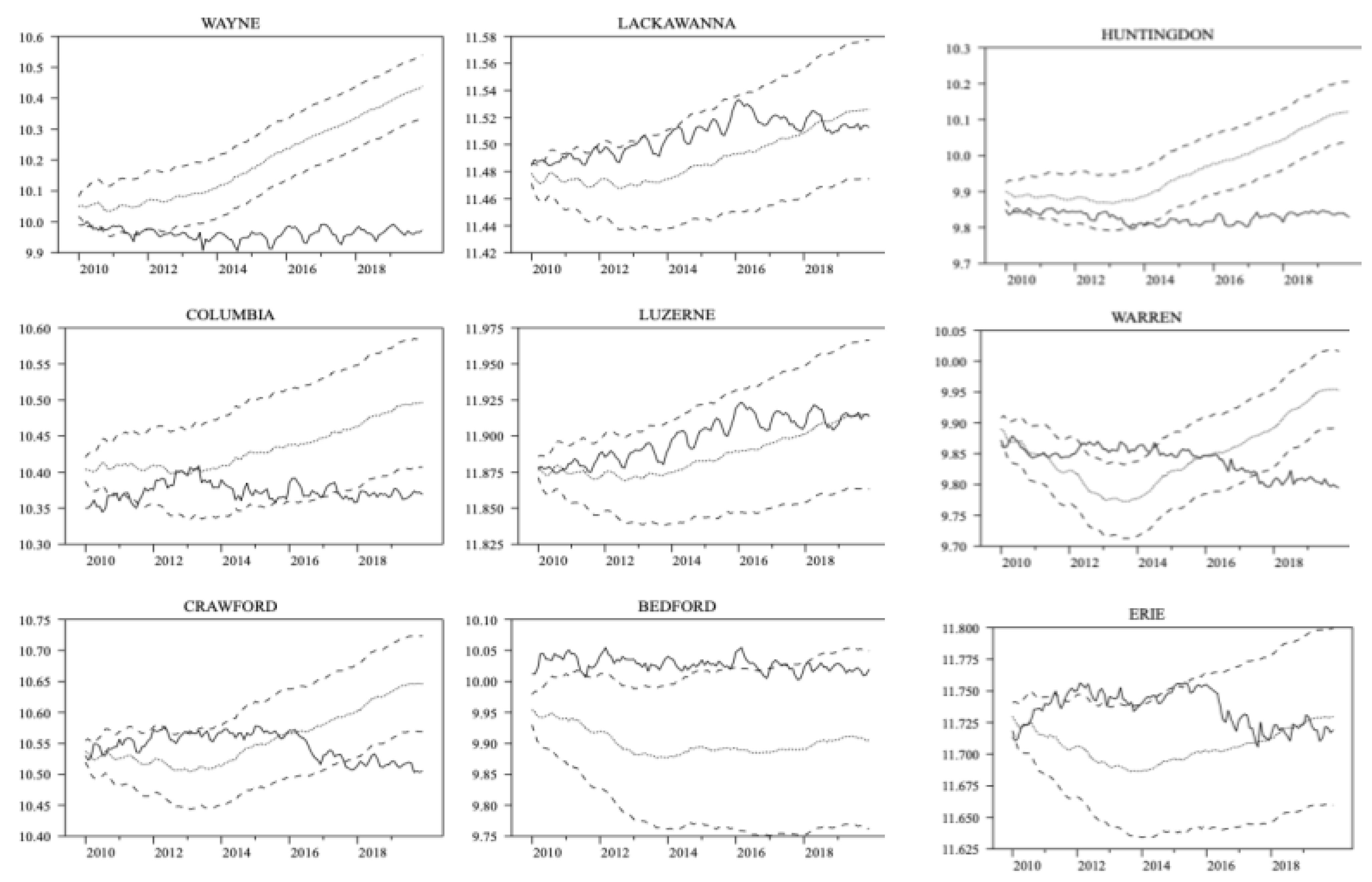
The results of the VAR models forecasted employment compared to actual employment are shown for each of the counties. To assist in seeing general patterns across the counties, these VARs are placed into bins. The 40 counties with drilling are grouped into five bins based on the total number of wells drilled reported in Table 1: 90th, 75th–89th, 50th–74th, 25th–49th, and 1st–24th percentiles. 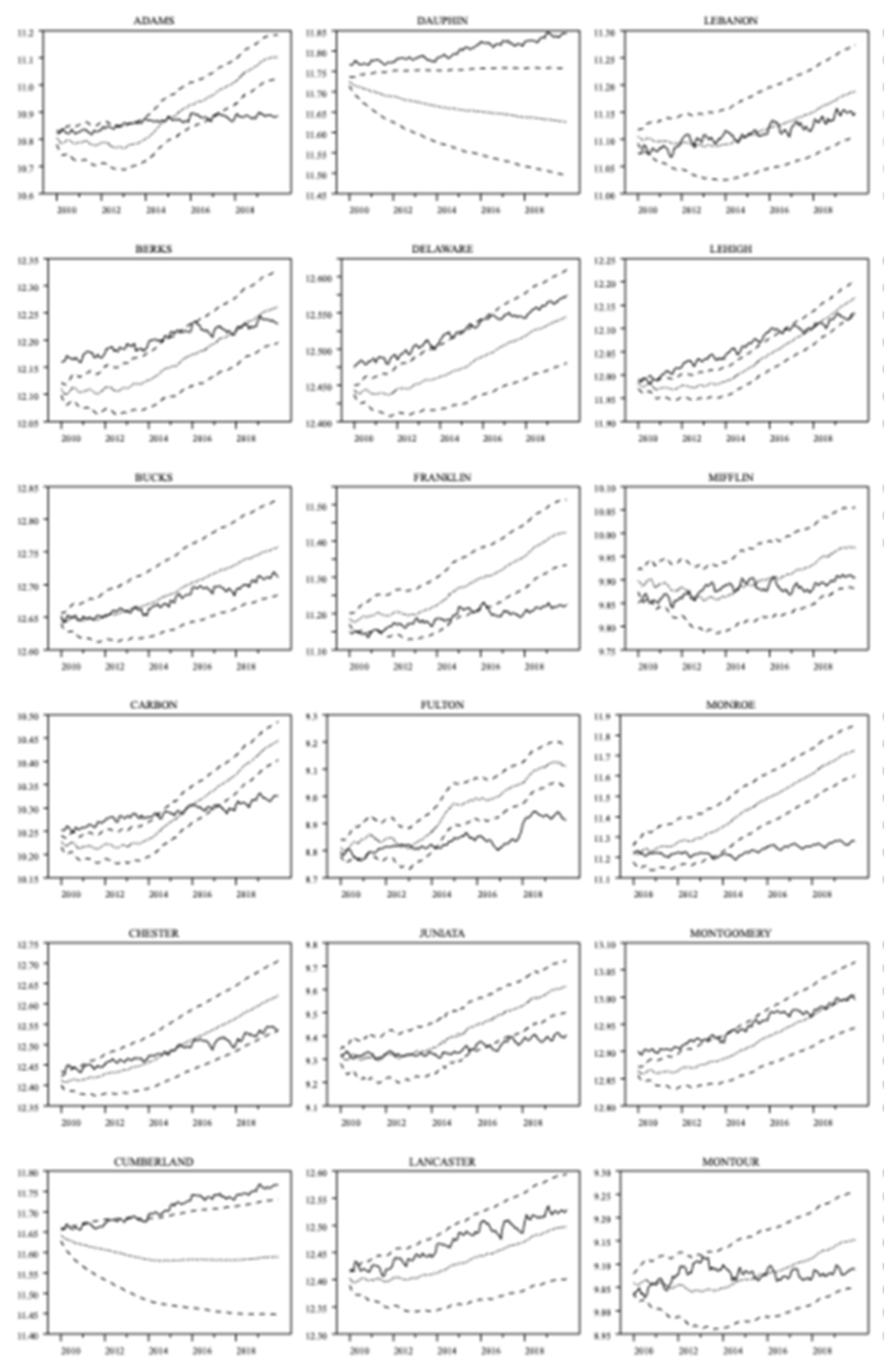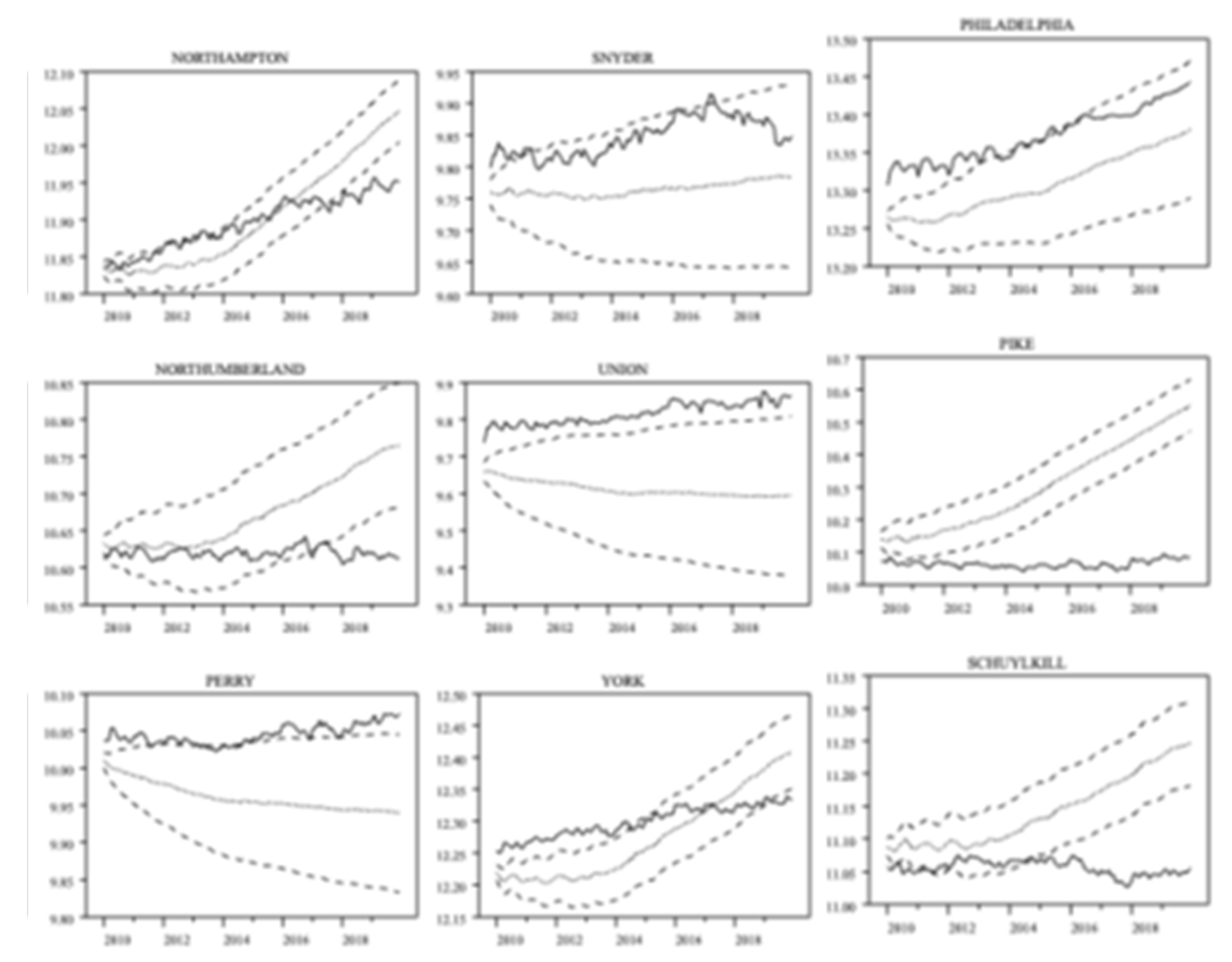These VARs are found in Figure 3, Figure 4, Figure 5, Figure 6 and Figure 7 below. Lastly, the VARs are shown for the 27 counties with no drilling, see Figure 8 below and Appendix A Figure A1. To aid readers in interpreting the VAR results and related analysis,

Table 4. Descriptive statistics for each drilling activity bin.

Percentile	Average Values per Bin				% Counties
	Total Wells	Wells per 100 k	2010–2020	Total
Grouping	Drilled	People	Pop. Change	Emp. 2023Q4	Urban
90th	1574	2646	−5.5%	28,725	0.0%
75–89th	600	855	−2.5%	47,544	16.7%
50–74th	147	643	−4.6%	72,846	20.0%
25–49th	35	68	−5.1%	25,154	0.0%
1–24th	2.3	3.2	−3.3%	46,059	30.0%
No Drill	0	0	2.40%	119,094	48.1%

provides several descriptive statistics for each of the groupings. There is much more drilling activity in the top quartile of drilling counties, especially within the top decile, than in the bottom 75 percent of drilling counties, so we expect positive employment effects to be most likely found in the top quartile.

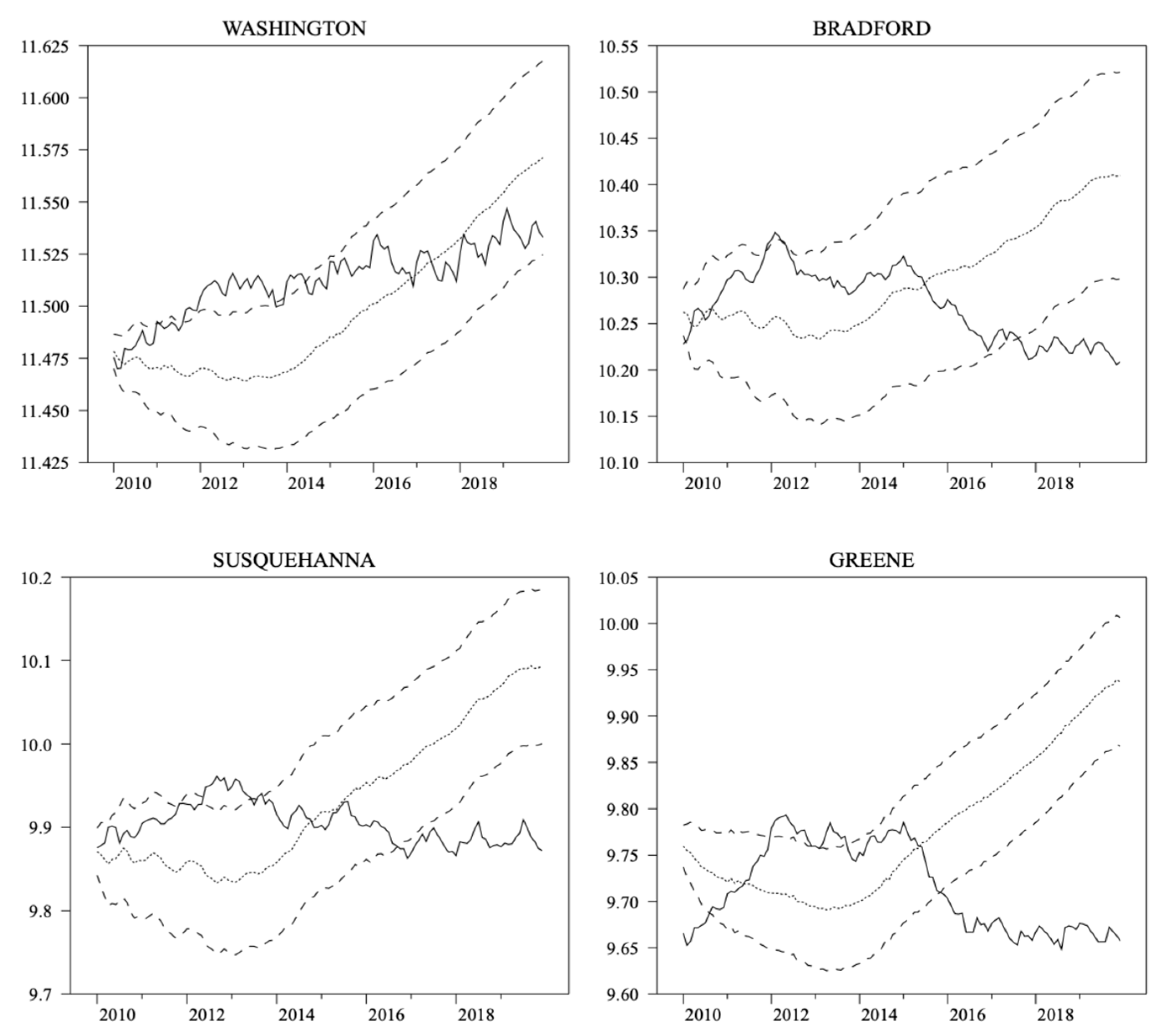
Figure 3 presents the actual time path of the log of employment for each county in the 90th percentile and above in drilling intensity (shown by the solid line) against its forecast and associated standard error bands, shown by the dashed lines. Washington county, which had the most unconventional wells developed over the relevant time period, did see employment levels consistently above forecast from around mid-2011 through the end of 2015 and saw employment above the upper standard error band from late 2011 to late 2013. Bradford and Susquehenna saw employment levels rise above the upper standard error band—briefly in 2011 for Bradford and in 2012 for Susquehenna—before ultimately falling back below forecast by 2014–2015. Greene county had employment levels well below forecast for most the months from 2010–2019, save for a three-year period from 2011–2014, in which its employment levels were above forecast, even breaking through the upper confidence band in 2012 and the first half of 2013. The results in Figure 3, taken as a whole, do seem to paint a picture that PA counties in the upper decile of unconventional drilling activity did have employment levels above forecast, some decidedly so, for at least some of the period from 2010–2019, usually during the 2011–2014 range and more consistently for Washington county.

Figure 4 presents the same information for the counties lying in the 75th–89th percentile for unconventional drilling activity. The two most heavily drilled counties in this grouping, Tioga and Lycoming, saw employment levels relative to forecast that were perhaps even better than that seen among the top decile of counties. For at least a few years, both experienced employment numbers that were comfortably above the forecast’s upper bound, meaning we can say these levels were higher than forecast and these deviations were indeed statistically significant. For Tioga, this positive difference occurred from roughly mid-2010 through mid-2013, whereas Lycoming had a longer such stretch, running from the beginning of 2011 through early 2015. Butler’s employment stayed very close to forecast for the entire sample period. Wyoming and Westmoreland experienced employment that exceeded forecast for most of the period in question, with Westmoreland eclipsing the forecast’s upper bound from 2012–2013. Fayette’s employment stayed substantially below even the lower bound the employment forecast every month from 2010–2019.

Figure 5 presents employment levels versus forecast for the ten counties in the 50th–74th percentile for number of unconventional wells drilled. Allegheny stands out in having employment levels above forecast in a statistically significant way for essentially the entire forecast period. It should be noted that Allegheny is the county housing the city of Pittsburgh, Pennsylvania’s second largest city and its urban anchor in the western part of the state. Armstrong, Elk, Cameron, and Potter saw employment eclipse the upper bound of the forecast interval for at least some portion during the first few years of the forecast horizon. Clinton and Beaver counties saw employment exceed forecast for substantial periods from 2011 to 2015 (2016 for Beaver) before falling below forecast for the latter part of the forecast period. Sullivan and McKean closely tracked their employment forecasts until 2015, when they began to lag substantially behind. Clearfield is the only county in this grouping whose actual employment levels were always below forecast for the entire 2010–2019 sample.

Figure 6 and Figure 7 are, of course, analogous to Figure 3, Figure 4 and Figure 5 but for the twenty counties in PA with the lowest number of unconventional wells drilled (but that did at least have one such well). Figure 6 presents findings for the 11 counties in the 25th–49th percentile for drilling activity and Figure 7 shows the same for the 9 counties in the 1st–24th percentile group. For all of the twenty counties combined in Figure 6 and Figure 7, eight experienced employment levels that were consistently above forecast: Mercer, Centre, Crawford, Warren, Bedford, Luzerne, Erie, and Lackawanna. Of these eight, Mercer, Bedford, and Erie had employment levels above the upper standard error band for substantial periods of time. Nine of the remaining twelve counties had employment levels within the standard error bands for the first 4–5 years of the forecast period before falling below the lower bound for roughly the latter half of the horizon. Blair and Jefferson counties are seen to stay near their forecasts for most of the forecast period.

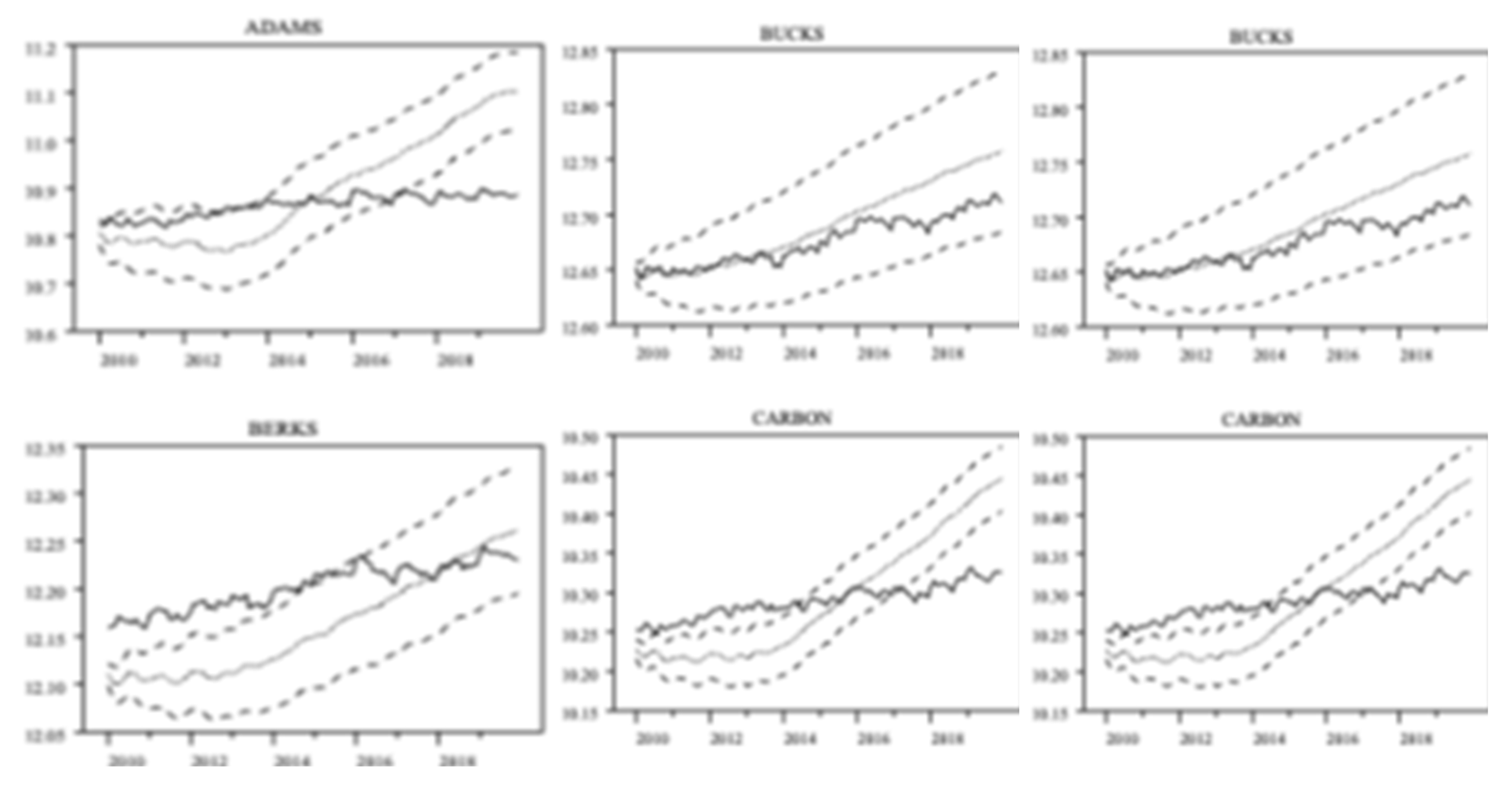
Finally, Figure 8 shows employment levels relative to forecast from 2010–2019 for 6 of the 27 counties in the state that had no drilling activity (all 27 counties shown in Appendix A, Figure A1). As before, a number of these counties have employment levels within the standard error bands until the latter portions of the forecast horizon. Others were seen to be above forecast for the entire sample, notably the urban counties in the southeast portion of the state: Berks, Delaware, Lehigh, and Philadelphia. The worst-performing counties relative to forecast among this group are Pike, Monroe, and Schuylkill, whose employment levels stayed consistently below forecast for the entire sample period and were often below the lower standard error band.

Figure 9 takes a portion of the information presented in Figure 3, Figure 4, Figure 5, Figure 6, Figure 7 and Figure 8 and presents it in a different way. The results shown thus far seem to indicate that most of the positive response from the fracking boom occurs in the first few years after the increase in exploration took place. Indeed, the information presented in

Table 5. Evolution of oil and gas industry in PA over the forecast horizon.

	PA GDP in NAICS 211	PA Employment	Unconventional Wells
Year	(Billions of Dollars)	(in NAICS 21)	Drilled in PA
2010	2.80	28,936	1600
2011	4.34	35,225	1958
2012	5.46	33,977	1351
2013	5.53	35,160	1213
2014	8.48	38,025	1369
2015	5.15	28,355	784
2016	4,76	23,822	502
2017	5.09	26,835	811
2018	5.06	28,685	780
2019	4.34	25,828	614
2020	3.14	20,971	476

Source: PA GDP data obtained from the St. Louis Federal Reserve (FRED), PA employment data from the PA Center for Workforce Information and Analysis, and drilling data from the PA Department of Oil and Gas Management.

indicates that after 2014, activity in the industry within the state began to sharply decline. We see that state GDP in NAICS 211 industries (oil and natural gas extraction) decreased by over 39% from 2014 to 2015. By 2020, such activity was only 37% of what it was at its peak. Similarly, state employment in NAICS 21 decreased by over 25% from 2014 to 2015 and stayed relatively subdued. Data on state employment in NAICS 211 was unavailable over the full 2010–2020 period, so we used NAICS 21, which also includes employment in mining. Moreover, Table 5 reports that the number of new unconventional wells drilled in the state fell by over 42% from 2014 to 2015, and by 2020, the number of new wells drilled was less than one-fourth what it was in 2011. As shown in Figure 9, we therefore decided to focus our attention on the first five years after the fracking boom. Specifically, we took each county’s employment deviation from forecast at various horizons (6, 12, 18, 24, 30, 36, 48, and 60 months) and computed the average deviation at each time horizon for the various percentile groupings for the drilling activity reported in Figure 3, Figure 4, Figure 5, Figure 6, Figure 7 and Figure 8 (90th and above, 75th–89th, 50th–74th, 25th–49th, 1st–24th, and ‘no drilling’). For example, Figure 9 shows that for counties with no drilling activity, the average employment deviation from forecast at the 6-month forecast horizon (June 2010) was just under 0.02 (2%). For the counties in the 90th+ percentile for drilling activity, the average employment deviation from forecast at the 24-month forecast horizon (which would amount to January 2012) was roughly 0.065 (6.5%). If one takes ‘no-drilling’ as the benchmark, then the percentile groups that consistently had a higher average employment deviation from forecast than counties with no drilling are the counties in the top half (50th percentile and above) of unconventional drilling activity. We present the results for non-drilling counties here for comparison purposes only, which is not to say that drilling counties should be expected to match the performance of their non-drilling counterparts. There are many other differences between drilling and non-drilling counties that could alter employment dynamics, not least of which is urban/rural designation. This study addresses this issue in more detail in Section 3.2. For the 90th percentile group and the 50th–75th percentile group, this over-performance takes place beginning at the 12-month forecast horizon. It takes until the 18-month horizon for the 75th–89th percentile group to outpace the non-drilling counties. Figure 9 illustrates that counties in the 1st–24th and the 25th–49th percentile groups never outperformed the non-drilling benchmark at any forecast horizon within five years after the fracking boom took place. Additionally, note that the relative employment benefit to fracking clearly seems to dissipate at the four-to-five-year forecast horizon, consistent with the findings presented thus far and of those uncovered by others.

To gain further insight into the relationship between drilling activity and county employment levels relative to what would have otherwise been forecast, we next take each county and examine the extent to which its actual employment was different from forecast for both the full ten-year span from 2010–2019 and the five-year span from 2010–2014. Specifically, for each county, for the ten-year forecast horizon, there are 120 monthly observations of employment deviations from forecast. Once we have these 120 observations for a specific county, we test the null hypothesis that the average of these deviations is different from zero and obtain the associated t-statistic. We then take the average of this t-statistic for the counties in each of the aforementioned percentile groupings based on drilling intensity and report them in Figure 10. Figure 10 also reports similar t-statistics for the smaller 5-year forecast horizon, which is obviously based on 60 observations of employment deviations from forecast for each county. Figure 10 shows that for the 5-year forecast horizon, every percentile group among drilling counties, save the 25th–49th percentile grouping, had positive t-statistics for this particular test, and these employment deviations were statistically significant at the 5% level. It should be noted, however, that the non-drilling group also had a positive t-statistic over this same hypothesis test and that the t-statistic for this group was actually higher than that for any of the drilling groups. For the full 10-year forecast horizon, the 75th–89th, 50th–74th, and the 1st–24th percentiles all had positive average t-statistics, but, once again, none of these values were higher than that for the non-drilling group of counties.

The results presented in Figure 10 are consistent with the general story told by Figure 9 and the numerous graphs of county employment level versus forecasts in Figure 3, Figure 4, Figure 5, Figure 6, Figure 7 and Figure 8: in terms of having actual employment levels post-fracking that were different from what would have otherwise been forecasted before the boom took place, counties that seemed to benefit from engaging in horizontal drilling were generally those in the upper half (50th percentile and above) in drilling activity in the state and that the relative employment benefit seemed to be more pronounced in the first five years of the initial increase in drilling activity. These results match those of Wrenn et al. [19], who found that only the most intensely drilled counties in PA saw an employment increase, and Komarek [23], who revealed that such employment benefits dissipated after three years. Recall that Jaenicke [20] and Gittings and Roach [21] also found modest positive employment effects from fracking in the Marcellus regions (although the response was muted when only local residents were counted in the employment numbers). Finally, these results also comport with Mayfield [22], who illustrate that most of the employment benefits of horizontal drilling in the Appalachian Basin accrued to rural areas but that such positive effects were generally short-lived.

4.2. Further Regression Analysis

For a final examination into the impact fracking had on employment deviations from forecast in Pennsylvania, we next perform a few straightforward ordinary least squares regressions. For each regression, the dependent variable is the estimated t-statistic for each county obtained from testing the hypothesis that the county’s employment deviation from forecast was different from zero. As before, we perform this for both the shortened 5-year forecast horizon from 2010–2014 (Table 5) and for the full 10-year forecast horizon from 2010–2019 (

Table 6. Regression results for OLS applied to Equations (2)–(5) for 5-year forecast horizon.

Estimation Results, Robust Standard Errors in III and IV
Dep. Var: t-Stat for Employment Deviation From Forecast
	Coefficient Estimates (std. errors in parentheses)
Independent Variable	I	II	III	IV
Intercept	17.9053 ***	9.622 *	2.051	4.94
	(5.531)	(5.026)	(3.476)	(4.215)
Drilling Dummy	−14.19 **	−8.487
	(4.27)	(5.64)
Urban Dummy		17.203 ***	22.0634 ***	15.31 *
		(6.138)	(6.517)	(8.269)
Wells Drilled per 100 k			0.0033 *	0.0048 **
			(0.0017)	(0.0019)
Pop. Growth				97.724
				(68.269)
R-squared	0.0919	0.1912	0.1751	0.1968
Adj. R-squared	0.0780	0.1659	0.1493	0.1585

Number of observations: 67, *: significant at 10% level, **: significant at 5% level, ***: significant at 1% level.

). We, of course, have one such t-statistic for each county, so our sample size for each regression is $n=67$. The larger the t-statistic is for a county, the more confident we can be that the county’s employment level over the forecast period was significantly different from forecast. Of course, large negative values for the t-statistic imply employment levels far below forecast. We wish to stress that our initial goal in these regressions is not to fully explain these t-statistics. There are myriad reasons why a specific county may or may not have outperformed its employment forecast over a 5- or 10-year period, and examining and modelling these factors would make up an entirely different project. We instead wish to see just how much of the deviation in these test statistics can be explained by fracking alone. Our first model is therefore extremely straightforward:

$$t_i={\beta }_0+{\beta }_1{D}_{drill,i}+{ϵ}_i$$

(3)

where $t_i$ is the t-statistic for county $i$ for the test of whether the county’s employment deviation from forecast over the relevant forecast horizon (either 5 or 10 years) was statistically significant, the $\beta s$ are coefficients, $D_{drill,i}$ is a dummy variable that equals ‘1’ if county $i$ engaged in any drilling at all and ‘0’ otherwise, and ${ϵ}_i$ is a Gaussian error term. The results from the estimation are presented in column ‘I’ of Table 6 and

Table 7. Regression results for OLS applied to Equations (2)–(5) for full 10-year forecast horizon.

Estimation Results, Robust Standard Errors in III and IV
Dep. Var: t-Stat for Employment Deviation from Forecast
	Coefficient Estimates (std. errors in parentheses)
Independent Variable	I	II	III	IV
Intercept	9.382 **	1.53	−2.394	−0.906
	(4.401)	(5.224)	(3.65)	(4.066)
Drilling Dummy	−10.271 *	−4.86
	(5.696)	(5.863)
Urban Dummy		16.307 **	18.685 ***	15.211 **
		(6.38)	(6.519)	(7.559)
Wells Drilled per 100 k			0.001	0.002
			(0.002)	(0.0019)
Pop. Growth				50.273
				(57.385)
R-squared	0.0476	0.1359	0.1277	0.1334
Adj. R-squared	0.033	0.1088	0.1004	0.0921

Number of observations: 67, *: significant at 10% level, **: significant at 5% level, ***: significant at 1% level.

(Table 6 for the 5-year forecast horizon and Table 7 for the full 10-year span). The results in Column I of Table 6 and Table 7 only tell us if a dummy indicating whether or not a county engaged in fracking activity can explain, in any meaningful way, its deviation from forecast over the specified forecast horizon. Examining the estimation results, we can see that the coefficient on the dummy variable indicating the presence of some drilling activity versus none is negative and statistically significant for both the full and shortened forecast horizons. Also, whether or not a county engaged in drilling accounted for only 9.2% of the variance in the t-statistic for whether its employment deviated from forecast over the 5-year forecast sample and only 4.7% over the full 10-year forecast span. This tells us that whether or not a county fracked or not can explain very little regarding its deviation from forecast over the specified time horizons. While the negative sign may be surprising, this simple model is surely suffering from omitted variable bias, as many other factors can influence a county’s employment relative to forecast other than simply whether or not it engaged in horizontal drilling.

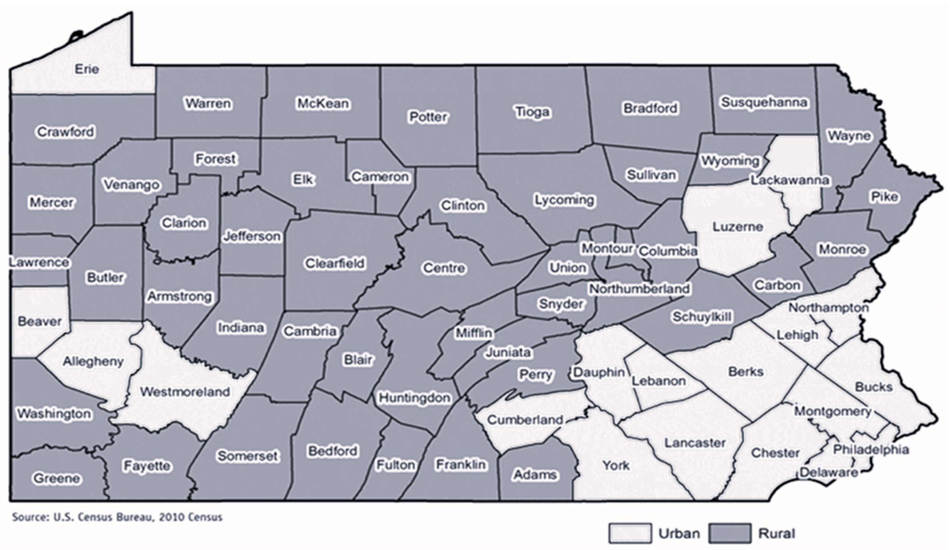
The next regression model we estimate simply adds another dummy variable to the model: one that is equal to ‘1’ if the county is labeled as ‘urban’ by the Center for Rural PA or ‘0’ otherwise:

$$t_i={\beta }_0+{\beta }_1{D}_{drill,i}+{\beta }_2{D}_{urban,i}+{ϵ}_i.$$

(4)

Column ‘II’ in Table 6 and Table 7 shows that adding the ‘urban’ dummy increases the $R^2$ to 0.1912 and 0.1359 (0.1659 and 0.1088, adjusted), respectively, for the 5-year and 10-year forecast horizon models. Furthermore, the coefficient on the new variable is positive and significant at the 1% level for both forecast horizons. The coefficient estimate on the drilling dummy loses its statistical significance once urban status is accounted for, indicating that some of the negative relationship between the drilling dummy and performance against forecast was reflecting the general under-performance of rural counties relative to urban ones in the state.

Next, to account for overall drilling intensity instead of simply whether or not a county had any drilling at all, we replace $D_{drill,i}$ with the number of wells drilled per 100 thousand residents in the county according to the 2010 U.S. Census ($WellsPerPo{p}_i$):

$$t_i={\beta }_0+{\beta }_{1}WellsPerPo{p}_i+{\beta }_2{D}_{urban,i}+{ϵ}_i.$$

(5)

These results are reported in Column ‘III’ of Table 6 and Table 7 and once again show the strong, positive employment response a county in PA had from 2010–2019 if it was urban instead of rural. The coefficient on drilling intensity is positive and statistically significant at the 10% level if only the first 5 years of the forecast horizon are analyzed. For the full 10-year horizon, the coefficient is positive but not statistically different from zero. These results indicate a modest but positive impact on employment deviations from forecast from increased drilling activity. As noted in Table 6’s heading, heteroskedasticity was detected in Equation (3)’s (as well as Equation (4)’s) specification, so White-heteroskedasticity-consistent standard errors were calculated. The low $R^2$s in these models underscore that only a small percentage of the variation in the dependent variable is accounted for by only drilling activity and urban/rural status, so clearly there are other factors that played a role in these employment deviations from forecast.

Finally, we add one more variable to the analysis that may be able to proxy for many exogenous factors that can influence whether or not a county outperformed its employment forecast: the county’s percentage change in its population over the 2010–2019 forecast horizon (reported in Table 1 and Table 2). The rationale is that if a county was experiencing population growth over this span, it may have been benefiting from some other outside factor that would have impacted its employment deviation. If its population shrunk over this span, it could have been suffering from some other negative factor that would have caused its employment to under-perform relative to forecast. Note that this approach is much more straightforward that that taken by researchers such as Cutler et al. [38], who use cointegration analysis to uncover underlying similarities between regional industry structures. This would allow for a potentially more informative control variable, but we leave such an exercise to future research. This new model is spelled out in Equation (6) and allows us to examine the extent to which drilling intensity increased employment relative to forecast when accounting for a county’s overall population change.

$$t_i={\beta }_0+{\beta }_{1}WellsPerPo{p}_i+{\beta }_2{D}_{urban,i}+{\beta }_{3}PopChang{e}_i+{ϵ}_i.$$

(6)

The estimation results when OLS is applied to Equation (6) can be found in Column IV of Table 6 and Table 7. One can see that when the shortened forecast horizon (Table 6) is utilized, drilling intensity is now positive and statistically significant at the 5% level. Urban status is still seen to impart a positive employment effect relative to forecast, but this impact is relatively lower once overall population growth is accounted for. There, of course, could be a degree of collinearity in play here, as the correlation between population growth and urban status is 0.684. When the full 10-year forecast horizon is analyzed, however, drilling intensity remains statistically insignificant, lending further evidence to the claim that any positive employment benefit from fracking tends to dissipate after 4–5 years.

While we are clearly not accounting for the myriad factors that may explain why counties may have had employment levels that were different from forecast from 2010–2019, we can use the results in Column ‘IV’ in Table 7 to perform a simple thought experiment. To be at least 95% sure a county had employment levels that were greater than forecast, one would need to see its t-statistic be 1.96. The results above reveal that an urban county with no drilling and a stable population would have a predicted t-statistic of $-906+15.211=14.305$, clearly above that needed for a p-value of 0.05. How about for a rural county? Our results indicate that each well drilled per one hundred thousand residents would raise the t-statistic by 0.002 (ignoring, for the moment, that this coefficient is not statistically significant from zero for when the full 10-year forecast horizon is employed). This finding means that a rural county with a stable population would have needed 1433 wells drilled per one hundred thousand residents to have a t-statistic of 1.96. This would have placed it 7th out of 40 drilling counties in wells drilled per one hundred thousand residents, further illustrating that only counties with very extensive drilling activity could have expected employment levels that were greater than would have otherwise been predicted had the fracking boom never taken place.

4.3. Limitations and Potential Future Research

This study’s use of parsimoneous VAR models allowing for lag structures unique to each county permits the labor market dynamics to vary across each county and examining the pattern of forecasted employment to actual employment across counties by their drilling activity is informative. The need for estimating and analyzing 67 separate VARs, however, limits the practicality of running several different versions of the VAR model for each county. One potentially fruitful area for future research using VAR models of employment would be to first restrict the analysis to just the counties with the most drilling activity. For these counties, a variety of VAR models could be employed, such as county-level controls related to age–structure, educational attainment, and industry composition; and macro-level controls, such as interest rates, consumer confidence, producer confidence, or national labor market variables. Alternatively, multiple contiguous counties with active drilling could be combined into a single VAR model that tests for spillover employment effects across counties from drilling.

Another approach would be to restrict the initial base period to end five years earlier in December 2004 and then forecast employment from 2005–2010, halting just before the drilling boom commenced in Pennsylvania. These “pre-boom” forecasts could be compared against actual employment and the results compared to those found in this paper. With regards to interpretation of the findings in this paper, a possible limitation is that no formal corrections are made for multiple testing adjustments for reported p-values. Fortunately, the pattern of which drilling counties ever show actual employment above the 95% confidence upper bound is unlikely to be materially impacted by Type-I errors. With 40 drilling counties, we can expect that two counties (0.05 × 40) falsely show actual employment above forecasted. Even if these two random outcomes happened to counties most actively drilled, it would not alter our main findings. First, drilling counties that ever showed actual employment above forecasted were more prevalent in high-drilling counties. Reviewing Figure 3, Figure 4, Figure 5, Figure 6 and Figure 7, seven of the ten counties with the most wells drilled had actual employment that exceeded forecast at some point, while only nine of the thirty remaining drilling counties had this result. Attributing two of the seven most drilled counties to Type-I error does not alter this pattern. Additionally, these types of Type-I errors are unlikely to impact the strong pattern that nearly all the positive employment effects dissipate within five years.

5. Conclusions

5.1. Weak Evidence of Sustainable Local Employment Gains

This paper examines not just if Pennsylvania counties engaging in horizontal fracturing experienced employment increases in the 10 years after the state’s fracking boom in 2010 but also if these potential gains were different from what otherwise would have been forecasted if you based those forecasts on data that prevailed before the boom occurred. In other words, is there evidence that the fracking boom led to long-term sustainable gains in employment for the local drilling areas? VARs were estimated for county employment levels and U.S. and PA economic activity for each of the 67 counties in Pennsylvania, and dynamic forecasts and associated standard error bands were then obtained for each county for the 2010–2019 period. Each county’s actual employment levels over the period were then compared to the forecasts and their associated standard error bands.

When counties are broken into percentile groups based on drilling intensity, this study finds that counties in the upper half of drilling intensity did often see employment levels that beat forecast but that the relative employment benefit typically ends in roughly three to four years, a result consistent with the boom–bust employment cycle noted in Mayfield (2019) [22]. Over longer time horizons, the relative employment benefit to fracking stands on much softer footing. This is highlighted in

Table 8. Actual versus forecasted employment for top 12 drilling counties per 100,000.

	Wells per	Ever Exceed	Last 1/2 Year
County	100 k People	95% Upper Bound	Exceed 95% UB	Rank
Susquehanna	3821.9	Y	2013.6	1
Greene	3484.5	Y	2014	2
Tioga	2494	Y	2014.6	3
Sullivan	2489.1	N		4
Bradford	2425.7	Y	2012.6	5
Cameron	1514.3	Y	2013	6
Wyoming	1114	N		7
Lycoming	876.8	Y	2015.6	8
Washinton	851.7	Y	2014.6	9
Potter	641.6	Y	2013	10
Elk	632.3	Y	2013	11
Armsrong	377.1	Y	2011	12

below, which summarizes VAR results for the 12 most drilled counties on a wells per 100,000 people basis (see Appendix A 

Table A1. Actual versus forecasted employment for all 40 drilling counties per 100,000.

	Wells per	Ever Exceed	Last 1/2 Year
County	100 k People	95% Upper Bound	Exceed 95% UB	Rank
Susquehanna	3821.9	Y	2013.6	1
Green	3484.5	Y	2014	2
Tioga	2494	Y	2014.6	3
Sullivan	2489.1	N		4
Bradford	2425.7	Y	2012.6	5
Cameron	1514.3	Y	2013	6
Wyoming	1114	N		7
Lycoming	876.8	Y	2015.6	8
Washington	851.7	Y	2014.6	9
Potter	641.6	Y	2013	10
Elk	632.3	Y	2013	11
Armstrong	377.1	Y	2011	12
Butler	336.1	N		13
McKean	313	N		14
Forest	285.1	N		15
Fayette	232.1	N		16
Clinton	196.2	N		17
Clearfield	175.2	N		18
Jefferson	121.7	N		19
Beaver	82.1	N		20
Lawrence	81.2	N		21
Westmoreland	78.1	Y	2013.6	22
Clarion	70	N		23
Mercer	52.3	Y	2013.6	24
Indiana	50.6	N		25
Centre	39	Y	2011	26
Somerset	30.9	N		27
Allegheny	13.2	Y	2019.6	28
Venango	10.9	N		29
Wayne	7.57	N		30
Warren	7.2	Y	2014.6	31
Cambria	4.9	N		32
Blair	4.72	N		33
Columbia	4.5	N		34
Crawford	3.4	Y	2012.6	35
Huntingdon	2.2	N		36
Bedford	2	Y	2017.6	37
Lackawanna	0.9	N		38
Luzerne	0.6	N		39
Erie	0.4	Y	2014.6	40

for all 40 counties with Marcellus shale drilling).

Findings of a positive impact from drilling activity upon employment are concentrated in just the most heavily drilled counties on a per 100,000 residents basis. For counties exceeding 350 drilled wells per 100,000 people over ten years, 10 of the 12 counties had some months with actual employment exceeding forecasted employment. For the 28 drilling counties with less than 350 drilled wells, only 8 ever had months with actual employment exceeding forecasted employment. Even for those most intensively drilled counties, the modest employment gains are temporary. For five of the ten counties, positive employment effects ended within three years, seven within four years, and nine within five years. There is no evidence from the VAR models of sustainable county employment gains across the counties in the Marcellus shale drilling region.

5.2. Negative Externalities Likely Impact Local Marcellus Shale Drilling Areas

As noted in the discussion of Table 7, an approximate calculation based on these final regression results is that a rural county with a stable population from 2010–2019 would have needed over 1433 wells drilled per 100,000 residents to be at least 95% certain its employment would have been higher than forecasted at some point from 2010–2019. As seen in Table 8, this amount of drilling intensity would have made it, on a per capita basis, the seventh most drilled county (out of the forty counties with drilling activity) in the state. Also keep in mind that these positive employment effects largely dissipate after four years.

Drilling 1433 wells per 100,000 residents is a substantial amount of drilling activity, which makes it ever more likely there are appreciable negative spillover effects related to health, environmental, and safety risks impacting these local drilling regions. This makes it doubtful that local drilling areas were moved onto more sustainable development paths. See Black [39] and Hendricks et al. [40] for systemic reviews of this literature. A few of the findings relevant to Marcellus shale region locales would include the road safety costs identified by Muehlenbachs, Staubli, and Chu [41], who estimated that in the county in which a Marcellus shale well is drilled, there are an additional 2798 truck trips within the county that year, a 2.5% rise in truck accidents, and a 1.2% rise in car accidents. Abramzon et al. [42] estimate that roadway consumptive use costs per Marcellus shale well drilled in Pennsylvania accounted for USD 13,000–USD 23,000 in damages. Graham et al. [43] found that heavily drilled counties in northern Pennsylvania had 15–23% higher vehicle crash rates in 2010–2012 and 61–65% higher heavy truck crash rates in 2011–2012 compared to control counties, while heavily drilled counties in southwestern Pennsylvania had 45–47% higher rates of fatal and major injury crashes in 2012 than in control counties. Clearly, heavy drilling activity exposes local residents to notable increases in crash risk and road degradation.

Heavy fracking activity also raises the risks of water contamination in the local drilling area; see Pan et al. [44] for a recent review of this water quality sustainability literature. Specific to this study, Entrekin et al. [45] note there were over 1400 drilling violations in Pennsylvania from January 2008 to October 2010, and nearly half of the violations were related to surface water contamination. These authors also note research indicating that only 10–30% of the fracture fluids typically were recovered from Marcellus shale wells. Risk assessment by Rozell and Reaven [46] of Marcellus shale drilling conclude that “even in a best-case scenario, it was very likely than an individual well would release at least 200 m³ of contaminated fluids.” In addition to localized water pollution risks, localized air pollution risks from Marcellus shale drilling have been documented. Litovitz et al. [47] estimate that in counties where drilling activities are concentrated, NO_x emissions were 20–40 times higher than what is permitted from a single point source. Moreover, most of these emissions are related to ongoing gas extraction and compression, so they will persist beyond the initial drilling period. Banan and Gernand [48] examine the impact of Marcellus shale drilling upon the drilling area population’s exposure to fine particulate matter (PM_2.5). They estimate that emissions from drilling activity, in addition to existing background, may have produced PM_2.5 concentrations exceeding the EPA standard for up to 36,449 persons per year from 2005–2017.

One potential localized health impact from pollutants related to Marcellus shale drilling is the increased risk to pregnant women and their babies. Hill [49] found that the introduction of drilling had a negative impact on mothers living within 2.5 km of a well compared to mothers living within 2.5 km of a future yet-to-be drilled well. An additional drilled well was associated with a 7 percent rise in low-birth-weight babies and a 3 percent rise in premature births. Analyzing Colorado data, Hill [50] finds that for mothers, residing within one kilometer of a well increases adverse birth outcomes and pregnancy complications compared to those residing 1–5 km away from a well. Other health risks associated with drilling activity are found in recent studies showing that close proximity to wells raises a variety of mental health risks [51,52,53], increases complications from severe asthma [54,55], and increases hospitalizations for heart attacks [56]. It is highly likely that these documented health risks from drilling activity were adversely impacting residents in the most intensively drilled Marcellus shale counties.

5.3. Contributions of This Paper to Sustainability Research on Impact of Fracking

The unique contribution of this research to the literature on sustainable energy development are the insights from the use of separate parsimonious VAR models of employment specific to each county in Pennsylvania. By allowing for different employment dynamics in each county, we find that only the most intensively drilled counties are likely to ever show months with actual employment above forecasted employment based on pre-drilling boom county labor dynamics. Most importantly, even for these counties, the impact is short-lived, dissipating within 4–5 years in nearly all cases. These results are consistent with other recent research that utilizes different estimation techniques.

Abboud and Betz [57] find that the “bust” periods lower county employment more than “boom” periods raise it when analyzing oil and gas booms across the U.S. Fleming-Munoz, and Poruschi [58] also found that employment gains eroded after several years when analyzing Australia’s natural gas boom. A possible reason for muted permanent employment gains is that some of the gains in local drilling-related employment come at the expense of local sectors. Gazal and Arano [59] document that gains in Marcellus shale employment within West Virginia led to lower forestry employment. This fits with Tsvetkova and Partridge [60], who find that after three years, oil and gas sector expansion tends to crowd out self-employment. Similarly, Huang and Etienne [61] find that shale gas development increased employment growth rates just in the short run for West Virginia and Pennsylvania. Young [62] examined if Pennsylvania’s Act 13 economic development funds collected from natural gas taxes and returned to counties based on drilling activity positively impacted county employment and found no effect.

Given that the wide range of documented risks and damages that can impact the population and environment of heavily drilled areas discussed in Section 5.2 can be long lasting, combined with this paper’s finding that the employment gains are temporary and modest, as discussed in Section 5.1, it seems unlikely that the rural counties in heavily drilled Marcellus shale areas have experienced a net gain in their county’s sustainability trajectory. These findings add support to the argument that sustainable development of additional electricity generation is more likely to be found in solar or wind power plus storage than in substantive expansions of natural-gas-fired electricity generation, even after accounting for employment gains in the natural gas producing areas. These findings will be of use to policymakers and citizens wishing to assess the likely sustainability impacts from shale gas drilling in a new region.