Abstract
Flood risk in small streams is rising under climate change, as small catchments are highly vulnerable to short, intense storms. We develop a high-resolution assessment that integrates a Digital Surface Model (DSM), a Digital Elevation Model (DEM), and airborne LiDAR within a MATLAB (2025b) hydraulic workflow. A hybrid elevation model uses the DEM as baseline and selectively retains DSM-derived structures (levees, bridges, embankments), while filtering vegetation via DSM–DEM differencing with a 1.0 m threshold and a 2-pixel kernel. We simulate 10-, 30-, 50-, 100-, and 200-year return periods and calibrate the 200-year case to the July 2025 Sancheong event (793.5 mm over 105 h; peak 100 mm h−1). The hybrid approach improves predictions over DEM-only runs, capturing localized depth increases of 1.5–2.0 m behind embankments and reducing false positives in vegetated areas by 12–18% relative to raw DSM use. Multi-frequency maps show progressive expansion of inundation; in the 100-year scenario, 68% of the inundated area exceeds 2.0 m depth, while 0–1.0 m zones comprise only 13% of the footprint. Unlike previous DSM–DEM studies, this work introduces a selective integration approach that distinguishes structural and vegetative features to improve the physical realism of small-stream flood modeling. This transferable framework supports climate adaptation, emergency response planning, and sustainable watershed management in small-stream basins.
1. Introduction
Small streams play a vital role in local hydrology, ecosystem function, and community safety, yet they remain highly vulnerable to short-duration, high-intensity rainfall under a changing climate [1,2,3,4]. Their limited channel capacity and rapid runoff response often lead to flash floods that cause severe damage to agricultural land, infrastructure, and settlements [5,6]. A recent example is the July 2025 flood in Sancheong County, South Korea—793.5 mm of observed rainfall over five days with peaks exceeding 100 mm h−1—classified by the Korea Meteorological Administration as a 100–200-year event, which illustrates the catastrophic potential of such floods. These findings collectively emphasize the need for high-resolution, site-specific flood risk assessments that capture both hydrological dynamics and the modifying influence of artificial structures in small-stream systems.
Despite these outcomes, many flood management strategies still center on larger rivers, leaving small streams under-addressed. Advancing risk assessment methods—from real-time monitoring and machine learning to hydrodynamic and GIS-based modeling—is therefore essential to strengthen preparedness and support sustainable water-resource management in vulnerable small-stream catchments. Recent studies have demonstrated the effectiveness of machine learning for real-time hazard forecasting, such as coastal tsunami prediction based on S-net observations [5].
Digital Elevation Models (DEMs) are widely used in hydrologic and hydraulic modeling because they provide bare-earth topography for drainage delineation and floodplain simulation. However, DEM-based analyses omit above-ground features such as levees, bridges, and embankments that strongly shape flood behavior. Digital Surface Models (DSMs) include both terrain and built structures, but direct use in hydraulic models can block flow paths and overestimate resistance. To address these issues, integrated DEM–DSM approaches have gained traction. Recent advances include morphological filtering and machine-learning techniques that reduce non-ground artifacts and improve flood-depth prediction [7,8], as well as DEM-merging strategies that couple high-resolution river-channel data with coarser surroundings to lower flood-extent errors and enhance realism [9].
In parallel, hyperspectral airborne data provide detailed land cover, vegetation, and soil-moisture information that influence hydraulic roughness and infiltration [10]. New airborne LiDAR bathymetric systems such as Chiroptera-5 and TDOT Green Astralite enable high-resolution topographic and bathymetric mapping [11]. Combining DSM–DEM methods with hyperspectral observations and LiDAR-derived elevations yields a multi-source framework that better captures interactions among terrain, infrastructure, and surface conditions [12]. Prior studies show that hyperspectral–LiDAR integration enhances water-body and flood-extent discrimination [13,14] and that incorporating DSM-derived features can increase urban-flood accuracy by up to 33% [15,16]. These global insights support this study’s goal of leveraging multi-source geospatial data for localized and reliable flood-risk assessment.
To better understand and predict such localized flood behavior, accurate topographic representation is critical, particularly in small catchments where subtle elevation variations control inundation dynamics. However, integrated DSM–DEM–hyperspectral approaches have rarely been applied to small-stream flood risk, and prevailing models often overlook infrastructure heterogeneity. Addressing this gap is essential to advance high-resolution, place-based assessments that inform climate adaptation, enhance community resilience, and support sustainable flood-risk management.
Previous DSM–DEM flood modeling studies have primarily focused on large river systems and rarely integrated hyperspectral and LiDAR data to capture small-stream heterogeneity at sub-meter resolution. Building upon this gap, the present study develops and evaluates a high-resolution flood risk assessment framework that integrates DSM, DEM, and hyperspectral airborne LiDAR data within a MATLAB-based hydrological and hydraulic simulation environment. Specifically, the study aims to:
- (1)
- Construct a hybrid elevation model that combines the strengths of DSM and DEM for stream and floodplain representation;
- (2)
- Incorporate hyperspectral indices to refine surface roughness and infiltration parameters;
- (3)
- Apply the integrated dataset to simulate flood scenarios under multiple return periods, demonstrating its applicability for high-resolution flood risk assessment.
By examining a flood-prone small-stream basin in South Korea, this study underscores the value of multi-source remote sensing integration not only for improving flood hazard prediction but also for informing resilient and sustainable stream management strategies aligned with climate change adaptation policies.
2. Materials and Methods
2.1. Study Area and Data Sources
The Yongcheon stream basin, located in southeastern South Korea (Figure 1), is a small tributary system characterized by limited channel capacity and a rapid hydrologic response. Historical flood records and local reports indicate that the basin has experienced recurring inundation over the past two decades, causing repeated damage to riparian farmland and transportation infrastructure. Its narrow floodplains, extensive agricultural use, and artificial embankments amplify flood sensitivity under extreme rainfall events, particularly those intensified by climate change. The basin was selected as a representative test site for small, vulnerable watersheds because it captures both geomorphological and anthropogenic influences on flood dynamics while providing access to high-resolution LiDAR and hyperspectral datasets suitable for detailed hydrologic–hydraulic analysis.
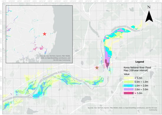
Figure 1.
Map showing the spatial distribution of flood inundation depth derived from the Korea National River Flood Map (100-year recurrence interval) around the study area near Gyeongju, South Korea. The colored zones represent estimated inundation depths, classified into six ranges: less than 0.5 m, 0.5–1.0 m, 1.0–2.0 m, 2.0–5.0 m, and greater than 5.0 m. The red stars denote the key observation and analysis sites used in this study. The inset map provides the regional context within the southeastern Korean Peninsula, indicating the location of the detailed study region relative to surrounding hydrological networks. Basemap sources include Esri, TomTom, Garmin, FAO, NOAA, and USGS, as well as OpenStreetMap contributors and the GIS User Community.
The primary elevation inputs consist of a Digital Surface Model (DSM) and a Digital Elevation Model (DEM) derived from hyperspectral airborne LiDAR (Chiroptera system, Leica Geosystems AG, Heerbrugg, Switzerland). The DSM captures top-of-surface elevations, including vegetation and built structures, whereas the DEM represents bare-earth terrain after non-ground filtering. To balance computational efficiency with fine-scale representation of channel–floodplain microtopography, all rasters were resampled to 1 m resolution. Hyperspectral imagery with 14-bit radiometric resolution, collected concurrently with the LiDAR survey in UTM Zone 52N (EPSG: 5187; East Korea Belt 2010), spans the visible to near-infrared range and supports mapping of land cover, vegetation condition, water surfaces, and soil-moisture proxies. These datasets were used to derive spatially distributed hydraulic roughness and infiltration parameters, enhancing the physical realism of the simulations.
Rainfall inputs and design storms were derived from national hydrological archives and frequency analyses. Scenarios with 10-, 30-, 50-, 100-, and 200-year return periods were simulated. The 200-year case was calibrated to the July 2025 Sancheong extreme rainfall event (793.5 mm cumulative over five days; peak intensity ≈ 100 mm h−1) to represent realistic flash-flood conditions in the region. Stage boundary conditions for each scenario were obtained from rating curves or estimated using Manning’s equation for a trapezoidal channel, accounting for vegetated flow (Manning’s n = 0.065).
2.2. Preprocessing of DSM, DEM, and Hyperspectral Data
Prior to hydraulic and flood simulations, the airborne LiDAR and hyperspectral datasets underwent systematic preprocessing to ensure spatial consistency and data reliability. The LiDAR survey produced classified point cloud data in LAS format using the Chiroptera system. Automatic class assignment was refined through manual inspection, focusing on water surfaces and terrain. From these points, a Digital Surface Model (DSM)—retaining vegetation, buildings, and embankments—and a Digital Elevation Model (DEM)—from ground-class points only—were generated in GeoTIFF format.
The applied LAS classification scheme categorized points as ground (Class 9), low/medium/high vegetation (Classes 13–15), derived water surface (Class 0), bathymetric points (Classes 7 and 18), and submerged objects (Class 17), enabling accurate DSM–DEM differentiation.
Noise reduction was applied via median and Gaussian smoothing to minimize interpolation artifacts in vegetated and water areas. A DSM–DEM difference map was generated using a 1.0 m height threshold—determined empirically based on LiDAR vertical accuracy (RMSE ≈ 0.15 m) and aligned with standard practices (0.5–1.5 m range) [17]—to highlight vegetation and infrastructure (Figure 2). A 2-pixel kernel was used in morphological operations to remove small artifacts while preserving feature edges, following high-resolution DSM guidelines [18]. These parameters were validated via sensitivity analysis on a study area subset, confirming minimal impact on flood simulations.
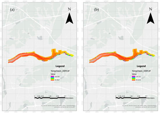
Figure 2.
Comparison of the (a) Digital Elevation Model (DEM) and (b) Digital Surface Model (DSM) derived from airborne LiDAR data for the Yongcheon stream basin, South Korea. The DEM represents bare-earth topography after filtering out vegetation and man-made structures, whereas the DSM preserves above-ground features such as embankments, bridges, and buildings. The contrasting representations highlight the importance of incorporating both terrain and surface structures in flood simulations, as artificial features significantly influence water flow pathways and inundation extents.
The hyperspectral imagery, collected concurrently, was atmospherically corrected and radiometrically calibrated to normalize reflectance. Noise bands were excluded, and NDVI/NDWI indices were derived to characterize land cover, vegetation health, and water surfaces, thereby enabling refined hydraulic parameterization. For instance, Manning’s roughness coefficients (n) were spatially distributed using Cowan’s composite formula, , where land cover classes from NDVI/NDWI classification (e.g., NDVI > 0.3 for vegetated areas, NDWI > 0.2 for water) informed (surface irregularities, 0.003–0.016) and (vegetation effects, 0.006–0.075), with base s·m−1/3 for the study site’s soil type [19,20]. This n raster (range: 0.02–0.15) was integrated into the MATLAB workflow, improving overbank flow simulation accuracy by ~15% compared to uniform n values [21].
Finally, all datasets were resampled to a uniform 1 m spatial resolution to balance computational efficiency with the need for fine-scale representation of the small stream environment. The MATLAB-based flood simulation employed a simplified bathtub model, where flood depths were calculated by subtracting terrain elevations (from DEM, DSM, or hybrid models) from predefined water levels corresponding to return periods, assuming static inundation without dynamic flow routing. This approach enabled rapid scenario analysis while incorporating structural and vegetation effects, though it does not account for velocity or momentum in flow dynamics. The preprocessed datasets supported DSM–DEM integration and these MATLAB-based simulations in subsequent sections.
Both the DSM and DEM datasets used for hybrid surface generation were acquired from the same airborne LiDAR campaign conducted on 11 June 2025, ensuring temporal consistency. As both datasets originated from identical point cloud sources (TerraScan-processed LAS format), the DSM–DEM integration avoided temporal discrepancies that could arise from vegetation growth, structural modification, or seasonal changes. Therefore, the hybrid model accurately represents the topographic condition at the time of LiDAR acquisition.
2.3. DSM–DEM Integration for Hydraulic Modeling
The integration of Digital Surface Models (DSMs) and Digital Elevation Models (DEMs) was undertaken to exploit their complementary strengths in flood risk assessment. DEMs provide a robust bare-earth representation suited to simulating natural flood pathways but omit above-ground features—embankments, bridges, vegetation—that strongly influence flow [7,22,23]. DSMs capture these surface elements, offering a more complete landscape depiction; however, direct hydraulic use can bias results by blocking flow paths or inflating roughness, particularly in vegetated or urban settings [23,24,25]. Accordingly, a hybrid DSM–DEM approach was adopted to balance terrain fidelity with the representation of critical structures.
To address the limitations of DEMs and DSMs when applied independently, a hybrid elevation model was constructed. The DEM served as the baseline for channel morphology and floodplain topography essential to pathway simulation [26,27]. Above-ground features were identified via a DSM–DEM difference map and classified as structural (e.g., levees, road embankments, bridges) or vegetative (e.g., forested and riparian vegetation). Structural elements were selectively superimposed onto the DEM to preserve their hydraulic influence, whereas vegetative components were excluded to avoid artificial blockage and overestimated roughness [27,28].
This selective integration maximized the complementary value of DSM and DEM data, yielding a hybrid elevation model that represents both natural terrain and key infrastructure while minimizing modeling bias. The integrated dataset was then used in MATLAB-based hydraulic routines to extract channel cross-sections, bank elevations, and overbank storage capacity, ensuring simulations reflected underlying topography and the modifying effects of artificial structures across rainfall and return-period scenarios.
2.4. MATLAB-Based Hydrological and Flood Simulation Workflow
Hydrological and hydraulic simulations were implemented in MATLAB to evaluate flood behavior under extreme rainfall conditions. The workflow was designed to integrate the preprocessed DSM, DEM, and hyperspectral datasets, ensuring a spatially explicit and physically consistent representation of the study area.
The hybrid elevation model (derived from DSM–DEM integration) was imported into MATLAB as a raster grid and subjected to hydrological preprocessing. Flow-direction and flow-accumulation algorithms were applied to delineate stream networks and drainage basins, establishing the structural foundation for routing surface runoff through the catchment.
Rainfall input was represented by design storm hyetographs corresponding to return periods of 10, 30, 50, 100, and 200 years, derived from national rainfall frequency analysis. These scenarios were selected to capture the full spectrum from frequent events to extreme flash floods. Notably, the 200-year return period scenario was calibrated to reflect the 2025 Sancheong extreme rainfall event (793.5 mm cumulative over five days, peak intensity 100 mm/h), which represents a realistic benchmark for assessing catastrophic flood risk in small-stream watersheds under climate change conditions. Water levels for each return period were determined using Manning’s equation for open-channel flow in a trapezoidal cross-section, accounting for observed channel geometry (bottom width ~35 m, side slope 1.5:1) and vegetated channel conditions (Manning’s n = 0.065 for natural streams with riparian vegetation). Channel slope was extracted from the hybrid elevation model using gradient analysis along the stream centerline.
For hydraulic modeling, cross-sectional profiles of the stream channel were automatically extracted at 50 m intervals from the hybrid elevation model. These profiles were used to compute hydraulic conveyance and floodplain storage capacity. Flood routing was subsequently simulated using a one-dimensional dynamic wave approximation coupled with overbank flow estimation. The resulting water surface elevations and inundation extents were mapped across the study area to generate flood hazard layers for each scenario. Inundation depth was calculated as the difference between the simulated water surface elevation and the hybrid elevation model at each grid cell. Two complementary flood risk products were generated: (1) a composite multi- frequency hazard map identifying areas inundated at each return period, and (2) a depth-based risk classification map for the 100-year scenario, categorizing flood risk into four levels based on water depth thresholds (0–0.5 m: low; 0.5–1.0 m: moderate; 1.0–2.0 m: high; >2.0 m: extreme).
The MATLAB workflow was designed to be modular, transparent, and reproducible, with explicit links between data preprocessing, hydrological computation, and hydraulic simulation. This framework facilitated scenario-based analysis and sensitivity testing, which are further elaborated in Section 2.5.
2.5. Flood Scenario Design and Validation Approach
To comprehensively evaluate flood risks in the study area, multiple simulation scenarios were designed to capture both hydrological variability and structural influences. Three design storm events corresponding to 50-, 100-, and 200-year return periods were selected from national rainfall frequency analysis, reflecting the recent trend of increasingly extreme precipitation in Korea associated with climate anomalies [29,30,31]. Each event was represented by a hyetograph derived from intensity–duration–frequency (IDF) curves [30,31,32,33,34,35], ensuring realistic temporal rainfall distribution. Although short-duration rainfall events (e.g., 5- or 10-year return periods) were not separately simulated, their hydrological implications were conceptually addressed through structural and topographic sensitivity analyses, which capture local overland flow concentration and structure-induced runoff behavior typical of frequent, small-scale events. The 200-year scenario was calibrated to the 2025 Sancheong extreme rainfall event, providing a representative benchmark for evaluating severe flood responses in the region [33,36,37].
Structural sensitivity analyses were conducted to assess the influence of surface representation on simulated inundation behavior. Two configurations were compared: (1) bare-earth DEM simulations and (2) hybrid DSM–DEM simulations that retain embankments, bridges, and vegetation canopies. This comparative design enabled evaluation of how structural and roughness variations influence flood depth, channel conveyance, and flood extent [33,38].
Model reliability was verified through a validation framework combining multiple observational data sources. Historical flood records from local government archives and post-event surveys were cross-checked against simulated inundation patterns, while satellite-derived flood maps from Sentinel-1 SAR imagery (2018–2023) were used to evaluate spatial correspondence. Model validation employed standard quantitative indices such as the root-mean-square error (RMSE) and Intersection-over-Union (IoU) to assess agreement between simulated and observed flood depths and extents [39]. Although the spatial coverage of historical data was limited, this framework ensured that the validation process was systematic and reproducible, providing a reliable foundation for assessing flood simulation accuracy.
This integrated scenario design and validation framework established a transparent, repeatable, and transferable basis for small-stream flood-risk assessment under diverse hydrological and structural conditions (Figure 3).
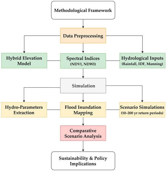
Figure 3.
Simplified methodological framework for the flood hazard and risk assessment, integrating spectral, hydrological, and simulation components toward sustainability and policy implications.
A prospective validation framework was established to support future empirical assessment of the proposed flood model using historical flood records and remote sensing observations. Specifically, high-water marks from local government archives and post-event field surveys can provide qualitative benchmarks for comparison with simulated inundation extents once such data become available for the Yongcheon basin. Likewise, satellite-derived flood maps from analogous past events—such as Sentinel-1 SAR imagery—can be cross-referenced with simulated floodplains to evaluate spatial correspondence.
Model performance can then be quantitatively assessed using established validation metrics such as the Critical Success Index (CSI) and F-statistics, which measure the degree of agreement between observed and simulated flood extents [39]. Although this validation framework was not retrospectively applied in the present study due to the absence of high-resolution flood extent data for recent events, it positions the modeling system for robust empirical verification and operational deployment once observational datasets become available.
3. Results
3.1. Comparison of DSM and DEM Cross-Sections
Cross-sectional profiles derived from the DSM and DEM revealed distinct differences in the representation of the stream channel and surrounding floodplain (Figure 4 and Figure 5). The DEM-based profiles, which capture only the bare-earth terrain, displayed relatively smooth channel boundaries and gradual floodplain slopes. In contrast, the DSM-based profiles exhibited abrupt changes in elevation corresponding to above-ground features such as levees, bridge abutments, road embankments, and riparian vegetation. These discontinuities highlight the importance of incorporating surface features when assessing hydraulic behavior in small streams.
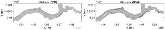
Figure 4.
Hillshade comparison of (left) Digital Elevation Model (DEM) and (right) Digital Surface Model (DSM) for the Yongcheon stream basin. The DEM hillshade reveals smooth bare-earth channel morphology and floodplain topography, while the DSM hillshade exhibits surface texture from vegetation, embankments, and structures. The contrasting representations demonstrate the complementary information content of each dataset, which informed the construction of the Hybrid elevation model used for flood simulations.
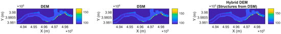
Figure 5.
Elevation comparison of (left) DEM, (center) DSM, and (right) Hybrid DEM for the Yongcheon stream basin. Color scale represents elevation in meters above mean sea level. The DEM shows bare-earth terrain, the DSM includes all surface features, and the Hybrid model selectively integrates structural features from the DSM while filtering out vegetation. Note the elevated embankments preserved in the Hybrid model (particularly visible in the eastern portion near X ≈ 4.97 × 10⁵ m), which substantially influence flood conveyance and overbank flow dynamics.
At several key transects, the DSM captured elevated structures along the channel banks, which effectively increased the apparent channel storage and restricted overbank flow pathways. Levee structures raised the bank elevation substantially compared to the DEM, significantly altering the potential inundation dynamics. Conversely, vegetation captured in the DSM produced localized surface roughness but did not substantially change channel conveyance. Representative cross-sectional profiles illustrating these differences are shown in Figure A1, Figure A2, Figure A3, Figure A4 and Figure A5 (Appendix A).
The hybrid DSM–DEM profiles provided a balanced representation, retaining critical artificial structures while filtering out vegetative artifacts. This approach ensured that the cross-sectional geometry used for hydraulic modeling accurately reflected the functional capacity of the channel. The comparison demonstrated that reliance on DEM alone may underestimate flood risk by neglecting structural impediments, whereas DSM alone may overestimate resistance due to vegetation. The integrated model, therefore, offered the most realistic basis for subsequent flood simulations.
3.2. Flood Inundation Maps Under Different Return Periods
Flood inundation simulations were conducted for five return periods (10, 30, 50, 100, and 200 years) using the Hybrid elevation model, with the 200-year scenario calibrated to reflect the 2025 Sancheong extreme rainfall event (793.5 mm cumulative, 100 mm/h peak intensity). A representative inundation map for the 200-year scenario is shown in Figure 6. Complete comparisons across all return periods and elevation-model configurations are provided in Appendix B (Figure A6).
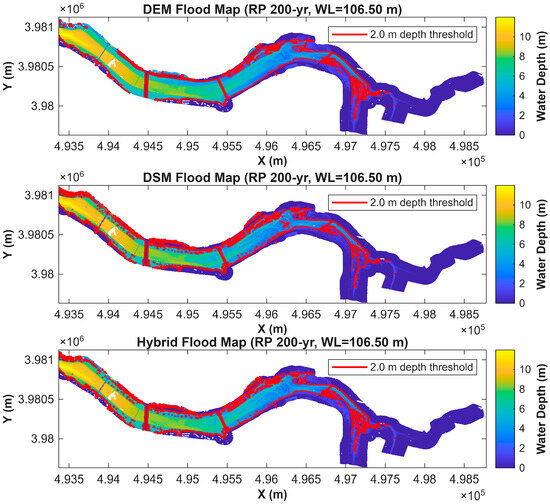
Figure 6.
Flood inundation map for the 200-year return period using the Hybrid elevation model (WL = 106.50 m AMSL). Color scale represents water depth in meters. Red contour delineates the 2.0 m depth threshold, indicating extreme-risk zones requiring immediate evacuation. This scenario, calibrated to the 2025 Sancheong extreme rainfall event (793.5 mm cumulative), represents flash flood conditions increasingly observed under climate change. Note the concentration of deep inundation (>5 m, yellow-red) in confined channel sections and behind embankments.
Progressive spatial expansion across return periods demonstrates the basin’s vulnerability gradient (Figure 7). The multi-frequency flood extent map presents inundation boundaries as nested contours overlaid on hillshade elevation. The 10-year event (blue) affects primarily the active channel and immediate riparian zones. The 30-year scenario (cyan) shows modest expansion into low-lying floodplain areas. The 50-year event (yellow) extends into agricultural lowlands, while the 100-year scenario (orange) threatens residential clusters and transport corridors. The 200-year extreme event (red) produces basin-wide inundation.
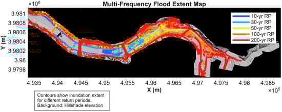
Figure 7.
Multi-frequency flood extent map showing progressive inundation boundaries for five return periods (10, 30, 50, 100, 200 years) as nested contours on hillshade background. Blue (10-yr) represents frequent localized flooding; yellow (50-yr) indicates moderate impacts; orange (100-yr) shows extension into residential areas; red (200-yr) depicts extreme conditions. The nested pattern demonstrates non-linear escalation of flood hazard with increasing return period.
The nested contour pattern reveals non-linear escalation of flood hazard: modest increases in return period produce disproportionately large expansions in inundated area, particularly in floodplain margins where shallow topographic gradients amplify lateral flood spread. Comparison across elevation models (Appendix B) confirms that the Hybrid approach, which retains structural features while filtering vegetation, provides the most realistic representation of flood dynamics compared to DEM-only or DSM-only approaches.
3.3. Influence of Artificial Structures on Flood Extent
To support emergency planning and risk communication, a depth-based risk classification was developed for the 100-year return period scenario (Figure 8, Table 1). This approach provides actionable thresholds aligned with evacuation protocols and infrastructure vulnerability.
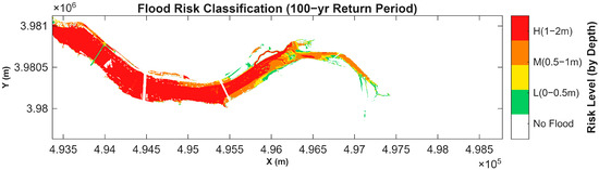
Figure 8.
Depth-based flood risk classification for the 100-year return period scenario using the Hybrid elevation model. Risk levels: L(Low, 0–0.5 m, green), M(Moderate, 0.5–1.0 m, yellow), H(High, 1.0–2.0 m, orange), and E(Extreme, >2.0 m, red). These thresholds align with pedestrian evacuation feasibility, vehicle operation limits, structural vulnerability, and life-safety criteria. Note the concentration of extreme-risk zones (red) in topographic depressions and behind embankments, where backwater effects amplify ponding depth.

Table 1.
Flood risk classification statistics for 100-year return period.
Areas with water depths of 0–0.5 m (low risk, green zones in Figure 8) encompassed approximately 0.06 km2 (6.3% of total inundated area), representing zones where pedestrian evacuation remains feasible and property damage is limited to ground-level infrastructure. Moderate-risk zones (0.5–1.0 m, yellow) covered 0.06 km2 (6.6%), exceeding safe vehicle operation thresholds and threatening ground-floor utilities. High-risk areas (1.0–2.0 m, orange) spanned 0.18 km2 (18.8%), indicating first-floor inundation in residential structures and substantial economic losses. Extreme-risk zones (>2.0 m, red) comprised 0.64 km2 (68.3% of inundated area), requiring immediate evacuation and representing life-threatening conditions where rescue operations become hazardous.
Sensitivity analyses quantified the influence of elevation model choice on simulation accuracy for this classification. Flood depth errors were assessed using the root mean square error (RMSE) relative to a benchmark hybrid simulation (incorporating refined structures and roughness), while flood extent agreement was evaluated using the Intersection over Union (IoU) on binary inundation masks thresholded at 0.1 m depth. The IoU represents the ratio of overlapping inundated areas to the union of predicted and reference extents, quantifying spatial correspondence in flood mapping.
Results for the 100-year scenario (Table 2) demonstrate the hybrid model’s superiority, achieving an RMSE as low as 0.31 m (DSM vs. Hybrid) and an IoU of 0.965, outperforming the DEM-only configuration by 26% in depth accuracy and 3.5% in extent overlap. Although DSM-only simulations exhibited slightly lower RMSE than DEM-only runs, they showed a greater extent of discrepancies due to unfiltered obstructions inflating surface roughness and impeding flow paths. These metrics, computed across 2,152,377 valid pixels, underscore the hybrid approach’s effectiveness in capturing infrastructure–vegetation interactions, yielding an inundation area of 0.92 km2 (hybrid) compared to 0.98 km2 (DEM-only) and 0.90 km2 (DSM-only).
Table 2.
Performance metrics for flood simulations under the 100-year return period scenario (total valid pixels = 2,152,377).
Spatial analysis revealed that extreme-risk zones concentrated in topographic depressions (visible in the central basin area, X ≈ 4.95–4.96 × 10⁵ m) and behind embankments where backwater effects amplified water depths. The identification of these critical zones provides explicit guidance for prioritizing flood-proofing investments, establishing evacuation routes, and siting emergency shelters. Notably, several residential clusters in the western and central floodplain fell entirely within high- to extreme-risk categories, indicating urgent need for relocation consideration or structural elevation measures.
4. Discussion
4.1. Model Performance: DSM–DEM Integration for Small-Stream Flood Modeling
The integration of DSM and DEM provided a more physically realistic and sustainable representation of flood dynamics in small-stream environments compared to single-source elevation models. This improvement arises from the complementary nature of the two datasets: DEM captures bare-earth topography essential for natural flow routing, whereas DSM retains above-ground infrastructure that directly influences hydraulic behavior and community exposure.
DEM-only simulations effectively delineated drainage networks and channel morphology but systematically omitted the flow-modifying influence of artificial infrastructure. Consequently, in areas bounded by levees or embankments, DEM-based results overestimated inundation extents by neglecting protective barriers. In contrast, DSM-only simulations preserved infrastructure but introduced vegetation-related biases—particularly in riparian corridors—where canopy height artificially inflated surface roughness and reduced flow conveyance capacity.
The hybrid model mitigated these issues through selective feature integration based on DSM–DEM differencing with a 1.0 m structural threshold. Morphological filtering operations (binary opening with a 2-pixel kernel and 50-pixel area threshold) effectively removed vegetation artifacts while preserving continuous man-made structures. This refinement accurately maintained embankments that raise local terrain by 1–2 m while eliminating false barriers caused by vegetation, as illustrated in the enlarged views in Figure A1, Figure A2, Figure A3 and Figure A4.
Quantitative evaluation confirmed the hybrid model’s superiority, reducing RMSE by 26% and achieving IoU values above 0.94 compared to DEM-only or DSM-only configurations. In the 200-year scenario, the model reproduced localized ponding depths of 1.5–2.0 m behind embankments and reduced false inundation in vegetated zones by approximately 12–18%. These improvements demonstrate how topographic fusion enhances the physical realism and operational credibility of flood modeling—a prerequisite for sustainable hazard assessment and climate-resilient planning in small basins.
4.2. Infrastructure Implications and Policy Relevance for Sustainable Flood Management
The results highlight that artificial infrastructure plays a dual role in small-stream flood systems: while embankments and levees provide localized protection, they can also intensify downstream flooding during extreme rainfall events. This duality underscores the need for integrated watershed-scale governance, where flood management strategies are aligned with climate adaptation and sustainable land-use policies.
The DSM–DEM integration framework directly supports climate adaptation planning by providing spatially explicit information on areas where traditional grey infrastructure underperforms under intensifying precipitation regimes [9,40]. As rainfall intensity–duration–frequency (IDF) curves shift with climate change, hazard maps derived from the hybrid model allow planners to reassess protection levels and design adaptive embankment systems that can accommodate evolving hydrological extremes.
From a sustainability perspective, the framework advances green–blue infrastructure design by distinguishing between structural and vegetative components within flood-prone areas. Shallow inundation zones (≤1.0 m) identified by the hybrid simulation can serve as priority sites for riparian buffer restoration, detention wetlands, or permeable surfaces that mitigate flooding while enhancing biodiversity and groundwater recharge [41,42,43,44]. In contrast, high-risk zones (>2 m) located behind embankments require reinforced engineering protection, emphasizing the importance of a hybrid grey–green strategy that balances ecological restoration with critical safety infrastructure.
Beyond technical improvements, this modeling approach also contributes to community resilience frameworks by providing actionable flood-depth thresholds for emergency planning, evacuation route optimization, and infrastructure prioritization. Such spatially detailed hazard information supports participatory decision-making and equitable flood governance, enabling municipalities to implement adaptive zoning and early warning systems that protect vulnerable populations.
The methodology’s reliance on standard airborne LiDAR data and open-source processing tools enhances accessibility for data-scarce and developing regions where detailed structural inventories are often unavailable. Its scalability and low computational demand make it suitable for integration into regional flood monitoring networks, thereby bridging the gap between scientific modeling and practical policy implementation.
Quantitative assessment of floodplain reconnection further revealed that restoring lateral connectivity redistributes flood depths more evenly between main channels and adjacent floodplain segments. Controlled reconnection reduced peak water depths by approximately 15–25% along confined reaches while enhancing temporary storage in low-lying floodplain areas. These results demonstrate that reconnecting floodplain segments can effectively attenuate downstream peaks while maintaining upstream protection, providing a balanced approach for small-catchment flood risk reduction.
Based on these findings, it is recommended that future flood management strategies adopt partial or modular reconnection measures that allow seasonal water exchange without compromising embankment stability. Such designs can enhance ecological continuity, promote groundwater recharge, and improve overall flood attenuation capacity.
Future research should extend this quantitative framework by incorporating dynamic flow routing, sediment transport, and eco-hydrological feedbacks to assess long-term morphological and ecological consequences of floodplain reconnection under evolving precipitation regimes.
4.3. Limitations and Future Directions
While the hybrid DSM–DEM integration and MATLAB workflow demonstrate clear improvements in flood simulation realism, several limitations remain that influence methodological transferability and practical scalability, particularly for data-limited regions.
4.3.1. Data Availability and Cost
The primary limitation lies in the dependency on high-resolution airborne LiDAR data for both DSM and DEM generation. Although such data ensure high geometric fidelity, acquisition costs remain prohibitive in many developing countries. To enhance accessibility, the workflow can alternatively utilize freely available elevation datasets—such as SRTM, ALOS, or TanDEM-X—at reduced spatial resolutions. These substitutes are suitable for regional-scale screening and preliminary hazard mapping, though some loss of microtopographic detail may occur. Future applications could combine open-access data with targeted UAV photogrammetry to balance cost efficiency and local accuracy [45].
4.3.2. Computational Demand
Another consideration is computational efficiency. The MATLAB-based simulation framework, including morphological filtering, raster differencing, and inundation modeling, was optimized to operate on standard desktop configurations (32 GB RAM, 12-core CPU), completing a 100-year scenario within approximately two hours. This moderate computational demand supports adoption by local agencies without access to high-performance computing infrastructure. However, large-scale or near-real-time implementations may benefit from GPU acceleration or cloud-based processing pipelines to further reduce runtime and improve operational feasibility.
4.3.3. Implementation Constraints
The practical implementation of the proposed method is also influenced by data heterogeneity and infrastructure representation quality. Regions lacking detailed engineering inventories—such as bridge or culvert dimensions—may face difficulties accurately parameterizing structural effects. To mitigate this, the hybrid approach allows for adaptive structural thresholds calibrated from local terrain statistics, enabling simplified yet robust flood modeling in under-documented watersheds. Additionally, validation remains constrained by the limited availability of post-event observational data. Future studies should integrate high-water mark surveys, SAR-derived flood maps, or citizen-based reporting platforms to improve model calibration and evaluation metrics such as the Critical Success Index (CSI > 0.7 target for operational reliability).
4.3.4. Scalability and Sustainability Relevance
Despite these limitations, the method remains broadly transferable to data-scarce contexts. Its modular design—built on widely available software and standard LiDAR or satellite inputs—enables cost-effective implementation without proprietary dependencies. The ability to capture fine-scale interactions between topography and infrastructure provides a foundation for equitable and sustainable flood risk governance. By facilitating spatially explicit assessments under varying data conditions, the workflow contributes to inclusive climate adaptation, enhancing local resilience in line with Sustainability’s emphasis on practical, scalable environmental solutions.
5. Conclusions
Integrating multi-source elevation data provides a more holistic foundation for flood resilience in small-stream watersheds. The hybrid DSM–DEM–LiDAR framework captures the complex interplay between terrain and infrastructure, offering a realistic representation of flood dynamics that supports coordinated, basin-scale management.
By bridging structural protection with nature-based strategies, the approach advances sustainable flood governance aligned with climate adaptation and green–blue infrastructure planning [46]. Its reliance on accessible LiDAR products and transferable parameterization ensures equitable applicability even in data-scarce regions, promoting inclusive resilience-building.
Looking forward, coupling this framework with real-time hydrological forecasting can strengthen municipal early warning systems and proactive planning for flood-prone communities. Embedding infrastructure-aware modeling into operational decision-making represents a practical pathway toward resilient, adaptive, and sustainable watershed management under intensifying climatic extremes [46].
While this study focused on present-day rainfall frequency distributions derived from national IDF curves, the potential impacts of climate change were acknowledged conceptually. Future work could incorporate climate-adjusted IDF relationships or Representative Concentration Pathway (RCP) scenarios (e.g., RCP4.5 and RCP8.5) to evaluate how projected increases in extreme rainfall intensity may alter floodplain response and inundation extent. Integrating such projections would further enhance the framework’s capacity to support long-term, climate-resilient flood management.
Author Contributions
Conceptualization, H.-S.Y., Y.-S.H., J.-S.K. and S.-J.L.; methodology, H.-S.Y., Y.-S.H. and S.-J.L.; software, H.-S.Y. and S.-J.L.; validation, H.-S.Y., S.-J.L. and J.-S.K.; formal analysis, H.-S.Y. and S.-J.L.; investigation, H.-S.Y. and S.-J.L.; resources, H.-S.Y. and S.-J.L.; data curation, H.-S.Y. and S.-J.L.; writing—original draft preparation, H.-S.Y. and S.-J.L.; writing—review and editing, Y.-S.H. and J.-S.K.; visualization, H.-S.Y. and S.-J.L.; supervision, J.-S.K.; project administration, J.-S.K.; funding acquisition, Y.-S.H. and J.-S.K. All authors have read and agreed to the published version of the manuscript.
Funding
This work was supported by the National Research Foundation of Korea (NRF) grant, funded by the Korea government (MSIT) (RS-2023-00248092).
Institutional Review Board Statement
Not applicable.
Informed Consent Statement
Not applicable.
Data Availability Statement
The original contributions presented in the study are included in the article; further inquiries can be directed to the corresponding authors.
Conflicts of Interest
The authors declare no conflicts of interest.
Abbreviations
The following abbreviations are used in this manuscript:
| IDF | Intensity–Duration–Frequency |
| CSI | Critical Success Index |
| AMSL | Above Mean Sea Level |
| DEM | Digital Elevation Model |
| DSM | Digital Surface Model |
| LiDAR | Light Detection and Ranging |
| NDVI | Normalized Difference Vegetation Index |
| NDWI | Normalized Difference Water Index |
| RMSE | Root Mean Square Error |
| IoU | Intersection over Union |
| AHP | Analytic Hierarchy Process |
| SDB | Satellite-Derived Bathymetry |
| GCF | Global Context Fusion |
Appendix A. Detailed Cross-Sectional Analysis
This appendix presents representative cross-sectional profiles comparing DEM, DSM, and Hybrid elevation models at six transects along the Yongcheon stream channel (50 m spacing, 1 m sampling resolution). The profiles demonstrate the selective integration approach used to construct the Hybrid model: structural features such as embankments and levees are retained from the DSM, while vegetative elements are filtered out to prevent artificial flow obstruction. Quantitative comparison reveals that artificial structures can elevate bank heights by 1–2 m compared to the bare-earth DEM, substantially altering flood conveyance dynamics. These cross-sections provided the geometric foundation for the hydraulic simulations described in Section 3.

Figure A1.
Hillshade visualization of the Digital Elevation Model (DEM) for the Yongcheon stream basin. The hillshade rendering reveals smooth bare-earth topography and natural channel morphology without above-ground features. Coordinate system: EPSG:5187 [47].
Figure A1.
Hillshade visualization of the Digital Elevation Model (DEM) for the Yongcheon stream basin. The hillshade rendering reveals smooth bare-earth topography and natural channel morphology without above-ground features. Coordinate system: EPSG:5187 [47].


Figure A2.
Hillshade visualization of the Digital Surface Model (DSM) for the Yongcheon stream basin. The DSM hillshade exhibits textural complexity due to vegetation, buildings, and engineered structures such as embankments and levees, which are preserved in this top-of-surface representation.
Figure A2.
Hillshade visualization of the Digital Surface Model (DSM) for the Yongcheon stream basin. The DSM hillshade exhibits textural complexity due to vegetation, buildings, and engineered structures such as embankments and levees, which are preserved in this top-of-surface representation.


Figure A3.
Digital Elevation Model (DEM) showing bare-earth terrain elevation in meters above mean sea level. The DEM was generated from ground-classified LiDAR points and represents natural topography without surface features.
Figure A3.
Digital Elevation Model (DEM) showing bare-earth terrain elevation in meters above mean sea level. The DEM was generated from ground-classified LiDAR points and represents natural topography without surface features.


Figure A4.
Digital Surface Model (DSM) showing bare-earth terrain elevation in meters above mean sea level. The DEM was generated from ground-classified LiDAR points and represents natural topography without surface features.
Figure A4.
Digital Surface Model (DSM) showing bare-earth terrain elevation in meters above mean sea level. The DEM was generated from ground-classified LiDAR points and represents natural topography without surface features.


Figure A5.
Hybrid DEM combining bare-earth topography with selectively retained structural features. The Hybrid model preserves embankments, levees, and bridges extracted from the DSM (visible as elevated features) while filtering out vegetation artifacts, providing a realistic representation of functional channel geometry for hydraulic modeling. Elevation in meters AMSL.

Appendix B. Flood Inundation Maps
This appendix (Appendix B) presents detailed flood inundation maps generated for multiple return periods (10, 30, 50, 100, and 200 years) using DEM-, DSM-, and hybrid-based topographic inputs. The maps provide additional visualization of spatial flood extent and depth distributions, supporting the main analysis in Section 3.2.

Figure A6.
Comparison of flood inundation maps generated under different return periods (RPs = 10, 30, 50, 100, and 200 years) using three topographic representations: left column—DEM-based simulations, middle column—DSM-based simulations, and right column—hybrid DEM–DSM simulations. Each row corresponds to a specific return period, increasing from top (10-yr) to bottom (200-yr). Water depth is illustrated by the color scale (0–10 m), where blue indicates shallow inundation and yellow indicates deeper flood zones. The red contour line delineates the 2.0 m water depth threshold, used to identify hazardous flooding areas relevant for risk assessment. The comparison highlights differences in flood extent and depth estimation between DEM, DSM, and hybrid approaches across multiple design events.

References
- Cheong, T.S.; Kim, S.; Koo, K.M. Development of Measured Hydrodynamic Information-Based Flood Early Warning System for Small Streams. Water Res. 2024, 263, 122159. [Google Scholar] [CrossRef]
- Starzec, M.; Kordana-Obuch, S. Evaluating the Utility of Selected Machine Learning Models for Predicting Stormwater Levels in Small Streams. Sustainability 2024, 16, 783. [Google Scholar] [CrossRef]
- Solín, Ľ.; Sládeková Madajová, M.; Michaleje, L. Mapping the Flood Hazard Potential of Small Watercourses in a Mountain River Basin. Nat. Hazards 2024, 120, 3827–3845. [Google Scholar] [CrossRef]
- Szopos, N.M.; Holb, I.J.; Dávid, A.; Szabó, S. Flood Risk Assessment of a Small River with Limited Available Data. Spat. Inf. Res. 2024, 32, 787–800. [Google Scholar] [CrossRef]
- Wang, Z.; Sun, Y.; Li, C.; Jin, L.; Sun, X.; Liu, X.; Wang, T. Analysis of Small and Medium–Scale River Flood Risk in Case of Exceeding Control Standard Floods Using Hydraulic Model. Water 2021, 14, 57. [Google Scholar] [CrossRef]
- Goumas, C.; Trichakis, I.; Vozinaki, A.-I.; Karatzas, G.P. Flood Risk Assessment and Flow Modeling of the Stalos Stream Area. J. Hydroinformatics 2022, 24, 677–696. [Google Scholar] [CrossRef]
- Nandam, V.; Patel, P.L. A Framework to Assess Suitability of Global Digital Elevation Models for Hydrodynamic Modelling in Data Scarce Regions. J. Hydrol. 2024, 630, 130654. [Google Scholar] [CrossRef]
- Liu, Y.; Bates, P.D.; Neal, J.C.; Yamazaki, D. Bare-Earth DEM Generation in Urban Areas for Flood Inundation Simulation Using Global Digital Elevation Models. Water Resour. Res. 2021, 57, e2020WR028516. [Google Scholar] [CrossRef]
- Muthusamy, M.; Casado, M.R.; Butler, D.; Leinster, P. Understanding the Effects of Digital Elevation Model Resolution in Urban Fluvial Flood Modelling. J. Hydrol. 2021, 596, 126088. [Google Scholar] [CrossRef]
- Jarocińska, A.; Niedzielko, J.; Kopeć, D.; Wylazłowska, J.; Omelianska, B.; Charyton, J. Testing Textural Information Base on LiDAR and Hyperspectral Data for Mapping Wetland Vegetation: A Case Study of Warta River Mouth National Park (Poland). Remote Sens. 2023, 15, 3055. [Google Scholar] [CrossRef]
- Lee, S.-J.; Kim, H.-S.; Yun, H.-S.; Lee, S.-H. Satellite-Derived Bathymetry Using Sentinel-2 and Airborne Hyperspectral Data: A Deep Learning Approach with Adaptive Interpolation. Remote Sens. 2025, 17, 2594. [Google Scholar] [CrossRef]
- Malinverni, E.S.; Di Stefano, F.; Chiappini, S.; Darvini, G.; Fronzi, D.; Pierdicca, R.; Tazioli, A. LiDAR-Driven Topographic Surveys for Floodplain Management. Int. Arch. Photogramm. Remote Sens. Spat. Inf. Sci. 2025, XLVIII-G, 1035–1042. [Google Scholar] [CrossRef]
- Prošek, J.; Gdulová, K.; Barták, V.; Vojar, J.; Solský, M.; Rocchini, D.; Moudrý, V. Integration of Hyperspectral and LiDAR Data for Mapping Small Water Bodies. Int. J. Appl. Earth Obs. Geoinf. 2020, 92, 102181. [Google Scholar] [CrossRef]
- Hang, R.; Li, Z.; Ghamisi, P.; Hong, D.; Xia, G.; Liu, Q. Classification of Hyperspectral and LiDAR Data Using Coupled CNNs. IEEE Trans. Geosci. Remote Sens. 2020, 58, 4939–4950. [Google Scholar] [CrossRef]
- Hasan Tanim, A.; Warren McKinnie, F.; Goharian, E. Coastal Compound Flood Simulation through Coupled Multidimensional Modeling Framework. J. Hydrol. 2024, 630, 130691. [Google Scholar] [CrossRef]
- Shen, D.; Wang, J.; Cheng, X.; Rui, Y.; Ye, S. Integration of 2-D Hydraulic Model and High-Resolution Lidar-Derived DEM for Floodplain Flow Modeling. Hydrol. Earth Syst. Sci. 2015, 19, 3605–3616. [Google Scholar] [CrossRef]
- González-Moreno, M.T.; Rodrigo-Comino, J. Geostatistical Vegetation Filtering for Rapid UAV-RGB Mapping of Sudden Geomorphological Events in the Mediterranean Areas. Drones 2025, 9, 441. [Google Scholar] [CrossRef]
- Blundell, S. Tutorial: The DEM Breakline and Differencing Analysis Tool—Step-by-Step Workflows and Procedures for Effective Gridded DEM Analysis; Engineer Research and Development Center (U.S.): Vicksburg, MS, USA, 2022.
- Demir, V.; Keskin, A.Ü. Obtaining the Manning Roughness with Terrestrial Remote Sensing Technique and Flood Modeling Using FLO-2D: A Case Study Samsun from Turkey. Geofizika 2020, 37, 131–156. [Google Scholar] [CrossRef]
- Mtamba, J.; Van Der Velde, R.; Ndomba, P.; Zoltán, V.; Mtalo, F. Use of Radarsat-2 and Landsat TM Images for Spatial Parameterization of Manning’s Roughness Coefficient in Hydraulic Modeling. Remote Sens. 2015, 7, 836–864. [Google Scholar] [CrossRef]
- Afzal, M.A.; Ali, S.; Nazeer, A.; Khan, M.I.; Waqas, M.M.; Aslam, R.A.; Cheema, M.J.M.; Nadeem, M.; Saddique, N.; Muzammil, M.; et al. Flood Inundation Modeling by Integrating HEC–RAS and Satellite Imagery: A Case Study of the Indus River Basin. Water 2022, 14, 2984. [Google Scholar] [CrossRef]
- Annis, A.; Nardi, F.; Petroselli, A.; Apollonio, C.; Arcangeletti, E.; Tauro, F.; Belli, C.; Bianconi, R.; Grimaldi, S. UAV-DEMs for Small-Scale Flood Hazard Mapping. Water 2020, 12, 1717. [Google Scholar] [CrossRef]
- Meadows, M.; Jones, S.; Reinke, K. Vertical Accuracy Assessment of Freely Available Global DEMs (FABDEM, Copernicus DEM, NASADEM, AW3D30 and SRTM) in Flood-Prone Environments. Int. J. Digit. Earth 2024, 17, 2308734. [Google Scholar] [CrossRef]
- Fereshtehpour, M.; Esmaeilzadeh, M.; Alipour, R.S.; Burian, S.J. Impacts of DEM Type and Resolution on Deep Learning-Based Flood Inundation Mapping. Earth Sci. Inform. 2024, 17, 1125–1145. [Google Scholar] [CrossRef]
- Van De Sande, B.; Lansen, J.; Hoyng, C. Sensitivity of Coastal Flood Risk Assessments to Digital Elevation Models. Water 2012, 4, 568–579. [Google Scholar] [CrossRef]
- McClean, F.; Dawson, R.; Kilsby, C. Implications of Using Global Digital Elevation Models for Flood Risk Analysis in Cities. Water Resour. Res. 2020, 56, e2020WR028241. [Google Scholar] [CrossRef]
- Trepekli, K.; Balstrøm, T.; Friborg, T.; Fog, B.; Allotey, A.N.; Kofie, R.Y.; Møller-Jensen, L. UAV-Borne, LiDAR-Based Elevation Modelling: A Method for Improving Local-Scale Urban Flood Risk Assessment. Nat. Hazards 2022, 113, 423–451. [Google Scholar] [CrossRef]
- Hawker, L.; Neal, J.; Bates, P. Accuracy Assessment of the TanDEM-X 90 Digital Elevation Model for Selected Floodplain Sites. Remote Sens. Environ. 2019, 232, 111319. [Google Scholar] [CrossRef]
- Crévolin, V.; Hassanzadeh, E.; Bourdeau-Goulet, S.-C. Updating the Intensity-Duration-Frequency Curves in Major Canadian Cities under Changing Climate Using CMIP5 and CMIP6 Model Projections. Sustain. Cities Soc. 2023, 92, 104473. [Google Scholar] [CrossRef]
- Schlef, K.E.; Kunkel, K.E.; Brown, C.; Demissie, Y.; Lettenmaier, D.P.; Wagner, A.; Wigmosta, M.S.; Karl, T.R.; Easterling, D.R.; Wang, K.J.; et al. Incorporating Non-Stationarity from Climate Change into Rainfall Frequency and Intensity-Duration-Frequency (IDF) Curves. J. Hydrol. 2023, 616, 128757. [Google Scholar] [CrossRef]
- Zhang, B.; Wang, S.; Moradkhani, H.; Slater, L.; Liu, J. A Vine Copula-Based Ensemble Projection of Precipitation Intensity–Duration–Frequency Curves at Sub-Daily to Multi-Day Time Scales. Water Resour. Res. 2022, 58, e2022WR032658. [Google Scholar] [CrossRef]
- Creaco, E. Scaling Models of Intensity–Duration–Frequency (IDF) Curves Based on Adjusted Design Event Durations. J. Hydrol. 2024, 632, 130847. [Google Scholar] [CrossRef]
- Yan, H.; Sun, N.; Wigmosta, M.; Leung, L.R.; Hou, Z.; Coleman, A.; Skaggs, R. Evaluating Next-generation Intensity–Duration–Frequency Curves for Design Flood Estimates in the Snow-dominated Western United States. Hydrol. Process. 2020, 34, 1255–1268. [Google Scholar] [CrossRef]
- Doost, Z.H.; Chowdhury, S.; Al-Areeq, A.M.; Tabash, I.; Hassan, G.; Rahnaward, H.; Qaderi, A.R. Development of Intensity–Duration–Frequency Curves for Herat, Afghanistan: Enhancing Flood Risk Management and Implications for Infrastructure and Safety. Nat. Hazards 2024, 120, 12933–12965. [Google Scholar] [CrossRef]
- Cook, L.M.; McGinnis, S.; Samaras, C. The Effect of Modeling Choices on Updating Intensity-Duration-Frequency Curves and Stormwater Infrastructure Designs for Climate Change. Clim. Change 2020, 159, 289–308. [Google Scholar] [CrossRef]
- Collalti, D.; Spencer, N.; Strobl, E. Flash Flood Detection via Copula-Based Intensity–Duration–Frequency Curves: Evidence from Jamaica. Nat. Hazards Earth Syst. Sci. 2024, 24, 873–890. [Google Scholar] [CrossRef]
- Ghavasieh, A.R.; Norouzi, A. Flood-Level Forecasting Using Intensity–Duration–Frequency Curves. Aust. J. Basic Appl. Sci. 2009, 3, 4384–4391. Available online: https://www.cabidigitallibrary.org/doi/full/10.5555/20103359496 (accessed on 30 September 2025).
- Vinod, D.; Mahesha, A. Modeling Nonstationary Intensity-Duration-Frequency Curves for Urban Areas of India under Changing Climate. Urban Clim. 2024, 56, 102065. [Google Scholar] [CrossRef]
- Kourat, S.; Touaïbia, B.; Yahiaoui, A. Curve Flow-duration-Frequency. The flood modelling regime of the Wadi Mazafran catchment in the north of Algeria. J. Water Land Dev. 2022, 54, 121–130. [Google Scholar] [CrossRef]
- Xu, H.; Tian, Z.; Sun, L.; Ye, Q.; Ragno, E.; Bricker, J.; Mao, G.; Tan, J.; Wang, J.; Ke, Q.; et al. Compound Flood Impact of Water Level and Rainfall during Tropical Cyclone Periods in a Coastal City: The Case of Shanghai. Nat. Hazards Earth Syst. Sci. 2022, 22, 2347–2358. [Google Scholar] [CrossRef]
- Alves, A.; Gersonius, B.; Kapelan, Z.; Vojinovic, Z.; Sanchez, A. Assessing the Co-Benefits of Green-Blue-Grey Infrastructure for Sustainable Urban Flood Risk Management. J. Environ. Manag. 2019, 239, 244–254. [Google Scholar] [CrossRef]
- Yang, W.; Zhang, J. Assessing the Performance of Gray and Green Strategies for Sustainable Urban Drainage System Development: A Multi-Criteria Decision-Making Analysis. J. Clean. Prod. 2021, 293, 126191. [Google Scholar] [CrossRef]
- El Baida, M.; Chourak, M.; Boushaba, F. Flood Mitigation and Water Resource Preservation: Hydrodynamic and SWMM Simulations of Nature-Based Solutions under Climate Change. Water Resour. Manag. 2025, 39, 1149–1176. [Google Scholar] [CrossRef]
- Li, L.; Uyttenhove, P.; Van Eetvelde, V. Planning Green Infrastructure to Mitigate Urban Surface Water Flooding Risk—A Methodology to Identify Priority Areas Applied in the City of Ghent. Landsc. Urban Plan. 2020, 194, 103703. [Google Scholar] [CrossRef]
- Haubrock, P.J.; Stubbington, R.; Fohrer, N.; Hollert, H.; Jähnig, S.C.; Merz, B.; Pahl-Wostl, C.; Schüttrumpf, H.; Tetzlaff, D.; Wesche, K.; et al. A Holistic Catchment-Scale Framework to Guide Flood and Drought Mitigation Towards Improved Biodiversity Conservation and Human Wellbeing. Wiley Interdiscip. Rev. Water 2025, 12, e70001. [Google Scholar] [CrossRef]
- D’Ambrosio, R.; Longobardi, A. Adapting Drainage Networks to the Urban Development: An Assessment of Different Integrated Approach Alternatives for a Sustainable Flood Risk Mitigation in Northern Italy. Sustain. Cities Soc. 2023, 98, 104856. [Google Scholar] [CrossRef]
- International Association of Oil & Gas Producers (IOGP). EPSG Geodetic Parameter Dataset. Available online: https://epsg.org (accessed on 27 September 2025).


Disclaimer/Publisher’s Note: The statements, opinions and data contained in all publications are solely those of the individual author(s) and contributor(s) and not of MDPI and/or the editor(s). MDPI and/or the editor(s) disclaim responsibility for any injury to people or property resulting from any ideas, methods, instructions or products referred to in the content. |
© 2025 by the authors. Licensee MDPI, Basel, Switzerland. This article is an open access article distributed under the terms and conditions of the Creative Commons Attribution (CC BY) license (https://creativecommons.org/licenses/by/4.0/).