An Improved Equilibrium Optimizer for Solving Optimal Power Flow Problem

Abstract

With the rapid development of the economy, the quality of power systems has assumed an increasingly prominent influence on people’s daily lives. In this paper, an improved equilibrium optimizer (IEO) is proposed to solve the optimal power flow (OPF) problem. The algorithm uses the chaotic equilibrium pool to enhance the information interaction between individuals. In addition, a nonlinear dynamic generation mechanism is introduced to balance the global search and local development capabilities. At the same time, the improved algorithm uses the golden sine strategy to update the individual position and enhance the ability of the algorithm to jump out of local optimums. Sixteen benchmark test functions, Wilcoxon rank sum test and 30 CEC2014 complex test function optimization results show that the improved algorithm has better global searching ability than the basic equilibrium optimizer, as well as faster convergence and a more accurate solution than other improved equilibrium optimizers and metaheuristic algorithms. Finally, the improved algorithm is applied to the standard IEEE 30-bus test systems for different objectives. The obtained results demonstrate that the improved algorithm has better solutions than other algorithms in the literature for solving the optimal power flow problem.

1. Introduction

The main source of electricity in many countries is thermal power generation, which requires a large amount of nonrenewable resources such as coal. In recent decades, with rapid economic development, the scale of various fields has continued to increase, which has led to the increasingly large scale and complex structure of modern power systems. Optimal power flow (OPF) plays a crucial role in the complete operation of the power systems, power network planning and economic dispatching. The optimization of the OPF problem directly affects the life of urban and rural residents and the development of industry. Therefore, how to improve the power quality and economic benefits brought by the power system has attracted increasing attention.

The main goal of OPF is to achieve the optimal operating state by adjusting the control parameters of the power system [1,2,3,4,5,6]. The methods for solving the optimal power flow in power systems can be divided into traditional optimization algorithms and metaheuristic algorithms. Traditional optimization algorithms mainly include the gradient descent method [7], Newton method [8], linear programming [9] and interior point method [10]. These algorithms are characterized by their use of the objective function to solve the first- or second-order gradient of control variables. Because the OPF is a typically complex constrained, multi-extremum, nonlinear, nonconvex optimization problem, traditional optimization algorithms are generally trapped in local optima; hence, the optimization results depend greatly on the initial value in solving large-scale optimization problems. In recent years, researchers have proposed many metaheuristic algorithms by simulating various biological behaviors and physical phenomena in nature. These algorithms are widely used to solve problems related to power system optimization because of their simple structure, few adjustment parameters, and lack of need for gradient information. The metaheuristic algorithms commonly used to solve OPF problems include particle swarm optimization (PSO) [11], whale optimization algorithm (WOA) [12], marine predator algorithm (MPA) [13], salp swarm algorithm (SSA) [14], slime mould algorithm (SMA) [15], grasshopper optimization algorithm (GOA) [16], flower pollination algorithm (FPA) [17], sine–cosine algorithm (SCA) [18], etc. In addition, to solve the OPF problem in the power system more effectively, many scholars proposed improved metaheuristic algorithms. Khan et al. proposed a multi-objective hybrid firefly and particle swarm optimization (MOHFPSO) to solve OPF problems with different objectives [19]. Taher et al. proposed an improved moth flame optimization (IMFO) algorithm to effectively solve OPF problems [20]. Prasad et al. proposed a chaotic whale optimization algorithm (CWOA) for low accuracy the defect that the original WOA has in solving OPF problems [21]. Karimulla et al. proposed an enhanced sine–cosine algorithm (ESCA) to minimize power plant generation costs, losses, and emissions [22].

The equilibrium optimizer (EO) is a new metaheuristic algorithm proposed by scholar Faramarzia in 2019 [23]. The algorithm has been successfully applied in many fields because of its advantages such as few control parameters, excellent flexibility, and easy implementation. For example, Dinh et al. applied the EO algorithm to multimodal medical image fusion, effectively improving the quality of the fused image and preserving the edge information of the input image [24]. Salem et al. used the EO algorithm to solve the optimal power flow problem of the hybrid AC-DC grid, the goal of which is to minimize the total fuel cost, power generation emissions, power transmission loss and voltage deviation [25]. Elsheikh et al. used the EO algorithm to improve the random vector function connection network, to enhance the prediction ability of the laser cutting of polymethyl methacrylate sheets [26]. However, few scholars have proposed an improved EO algorithm to solve the OPF problems. Consequently, a method is made to improve the equilibrium optimizer to solve optimal power flow problems in power systems. The proposed algorithm uses the chaotic equilibrium pool to enhance the information interaction between individuals. Furthermore, a nonlinear dynamic generation mechanism is introduced to balance the global search and local development capabilities. In addition, the improved algorithm uses the golden sine strategy to update the individual position. In summary, the main contributions of this paper are as follows:

• An improvement in the efficiency of powerful metaheuristic method named EO is investigated to solve optimal power flow problems in the power system.
• An improved equilibrium optimizer algorithm called IEO, combined with a chaotic equilibrium pool, nonlinear dynamic generation mechanism and golden sine algorithm, is developed to enhance the ability of the original EO algorithm to handle complex optimization objectives. The performance of the IEO algorithm is evaluated on 16 benchmark test functions, the Wilcoxon rank sum test and well-known CEC2014 test functions.
• The proposed IEO algorithm is applied to solve optimal power flow problems in the standard IEEE 30-bus test system. The performance of the proposed IEO algorithm is investigated in terms of fuel cost, active power transmission loss, and voltage deviation improvement. The results are compared with those of other improved algorithms and metaheuristic algorithms in the literature.

The remainder of the paper is organized as follows: Section 2 addresses the OPF problem mathematically, including the objective functions, equality constraints, and inequality constraints. Section 3 describes the details of the proposed IEO algorithm, along with the mathematical model and computational process. Section 4 analyses the experimental results of the proposed IEO algorithm. Section 5 describes the comparative analysis between the proposed algorithm and other studies in the literature in solving OPF problems. The conclusion of this work is provided in Section 6.

2. OPF Problem Formulation

The optimal power flow problem is one of the most important problems faced by power system planners and operators, who aim to minimize an objective function by adjusting the control variables in the power system such as generation costs or active power transmission loss. The mathematics of the OPF problem can be represented using the following standard form:

$$Minimize F(x,u)$$

(1)

subject to

$$g(x,u)=0$$

(2)

$$h(x,u)\le 0$$

(3)

where F(x,u) represents the objective function of system optimization, u represents the vector of control variables consisting of the bus voltage values of generators, capacity of reactive power compensation, and transformer tap ratios, and x represents the vector of state variables including reactive power generations, voltage phase angle and voltage amplitude of each load bus. The function g(x,u) represents the equality constraints, and the function h(x,u) represents the inequality constraints.

2.1. Objective Function

In this paper, three objective functions consisting of fuel cost, active power transmission loss, and voltage deviation are considered as the objective functions in the OPF problem. The mathematical model of each objective function is as follows:

2.1.1. Fuel Cost (FC)

The total fuel cost of generator units is usually considered the most basic objective function in OPF research, where the cost curve of each generator unit is represented by a quadratic function. Therefore, the mathematical model of the total cost of fuel for electricity generation [13] is as follows:

$$F_1(x,u)={\displaystyle \sum _{i=1}^{Ng}\left(a_i+b_i{P}_{Gi}+c_i{P}_{Gi}^2\right)}$$

(4)

where $N_g$ is the number of generators, $a_i$, $b_i$, and $c_i$ are the fuel cost coefficients of the ith generator unit, and $P_{Gi}$ is the real power generation of the ith generator.

2.1.2. Active Power Transmission Loss (APL)

To further reduce power generation costs along with real power generation, the active power transmission loss is considered as an objective function. The mathematical model of the active power transmission losses [13] is as follows:

$$F_2(x,u)={\displaystyle \sum _{i,j\in N_l}^{}{G}_{ij}\left(V_i^2+V_j^2-2V_i{V}_j\cos ({\theta }_{ij})\right)}$$

(5)

where $N_l$ is the number of transmission lines, $G_{ij}$ is the transfer conductance of line ij, $V_i$ is the voltage amplitude at the ith bus, $V_j$ is the voltage amplitude at the jth bus, and cos(θ_ij) is the difference of the voltage phase angle between buses i and j.

2.1.3. Voltage Deviation (VD)

To ensure stable operation of the power system, generally, the voltage deviation range must be within 5% of the standard value. Due to a sudden increase in load demand, insufficient reactive power support, circuit failure, and other reasons, the bus voltage may deviate. Therefore, the voltage deviation is often considered as one of the objective functions of the OPF problem, and its mathematical model is as follows:

$$F_3(x,u)={\displaystyle \sum _{i=1}^{Ng}\left|V_i-1\right|}$$

(6)

2.2. Contraints

OPF constraints can be classified into equality and inequality constraints, which are detailed in the following sections.

2.2.1. Equality Constraints

The equality constraints of the OPF problem are usually the power balance constraint of each bus, including the active power balance equation and the reactive power balance equation. Their mathematical models are as follows:

$$P_{Gi}-P_{Di}=V_i{\displaystyle \sum _{i,j=1}^N{V}_j\left(G_{ij}\cos ({\theta }_{ij})+B_{ij}\sin ({\theta }_{ij})\right)}$$

(7)

$$Q_{Gi}-Q_{Di}=V_i{\displaystyle \sum _{i,j=1}^N{V}_j\left(G_{ij}\sin ({\theta }_{ij})-B_{ij}\cos ({\theta }_{ij})\right)}$$

(8)

where $Q_{Gi}$ is the reactive power generation of the ith generator, $P_{Di}$ and $Q_{Di}$ are the active power and reactive power of the ith bus, respectively; N is the number of buses, $G_{ij}$ and $B_{ij}$ are the conductance and susceptance between buses i and j, respectively, and $V_i$ and $V_j$ are the voltage amplitudes of buses i and j, respectively.

2.2.2. Inequality Constraints

The inequality constraints of the OPF problem include the constraints of physical equipment in the power system and the constraints generated by ensuring the safe operation of the system. Their mathematical models are as follows:

$$P_{Gi}^{min}\le P_{Gi}\le P_{Gi}^{max} i=1,2,\dots ,N_g$$

(9)

$$Q_{Gi}^{min}\le Q_{Gi}\le Q_{Gi}^{max} i=1,2,\dots ,N_g$$

(10)

$$V_{Gi}^{min}\le V_{Gi}\le V_{Gi}^{max} i=1,2,\dots ,N_g$$

(11)

$$T_i^{min}\le T_i\le T_i^{max} i=1,2,\dots ,N_t$$

(12)

$$Q_{Ci}^{min}\le Q_{Ci}\le Q_{Ci}^{max} i=1,2,\dots ,N_c$$

(13)

$$V_{Li}^{min}\le V_{Li}\le V_{Li}^{max} i=1,2,\dots ,N_l$$

(14)

$$\left|S_{Li}\right|\le S_{Li}^{max}$$

(15)

where $N_t$ is the number of transformer buses, $N_c$ is the number of reactive power compensation buses, $N_l$ is the number of branches in the system, $P_{Gi}^{\mathit{max}}$ and $P_{\mathit{Gi}}^{\mathit{min}}$ are the upper and lower limits of the active power of the ith generator unit, respectively; $Q_{\mathit{Gi}}^{\mathit{max}}$ and $Q_{\mathit{Gi}}^{\mathit{min}}$ are the upper and lower limits of the reactive power of the ith generator unit, respectively; $V_{\mathit{Gi}}^{\mathit{max}}$ and $V_{\mathit{Gi}}^{\mathit{min}}$ are the upper and lower limits of the voltage of the ith generator unit, respectively; $T_i^{\mathit{max}}$ and $T_i^{\mathit{min}}$ are the upper and lower limits of the transformer, respectively, $Q_{\mathit{Ci}}^{\mathit{max}}$ and $Q_{\mathit{Ci}}^{\mathit{min}}$ are the upper and lower limits of reactive power compensation capacity, respectively; $V_{\mathit{Li}}^{\mathit{max}}$ and $V_{\mathit{Li}}^{\mathit{min}}$ are the upper and lower limits of the load voltage at the ith bus, respectively; and $S_{\mathit{Li}}$ is the transmission power of the ith branch, and $S_{\mathit{Li}}^{\mathit{max}}$ is the upper limit of the transmission power of the ith branch.

3. Improved Equilibrium Optimizer

3.1. Equilibrium Optimizer (EO)

The EO algorithm is derived from a physical model that controls the volume–mass dynamic balance. The model describes the physical processes that control the entry, exit and generation of mass within a volume. The model is generally described by a first-order ordinary differential equation, and its mathematical model [23] is as follows:

$$V\frac{dC}{dt}=Q{C}_{eq}-QC+G$$

(16)

where V is the control volume, C is the concentration, Q is the volumetric flow rate of the control volume, C_eq is the concentration at the equilibrium state, and G is the mass generation rate of the control volume.

The mathematical model is obtained by solving the differential equation derived from Equation (16):

$$C=C_{eq}+(C_0+C_{eq})F+\frac{G}{\beta }(1-F)$$

(17)

$$F=\exp (-\beta (t-t_0))$$

(18)

where $C_0$ is the initial concentration, $t_0$ is the initial start time, F is the exponential term coefficient, and β is the flow rate. Similar to other metaheuristic algorithms, the EO algorithm initializes candidate solutions randomly and its mathematical model is as follows:

$$C_i=C_{min}+ran{d}_i\times (C_{max}-C_{min})$$

(19)

where $C_i$ represents the position of the ith individual, ${\mathit{rand}}_i$ is a random number between [0, 1], and $C_{\mathit{max}}$ and $C_{\mathit{min}}$ are the upper and lower boundaries of the search space, respectively. $C_{\mathit{eq},\mathit{pool}}$ is the randomly selected solution from the equilibrium pool, which is constructed as follows:

$$C_{eq,pool}=\left\{C_{eq(1)},C_{eq(2)},C_{eq(3)},C_{eq(4)},C_{eq(ave)}\right\}$$

(20)

where $C_{\mathit{eq}\left(1\right)}$, $C_{\mathit{eq}\left(2\right)}$, $C_{\mathit{eq}\left(3\right)}$, $C_{\mathit{eq}\left(4\right)}$ are four best-so-far candidate solutions and $C_{\mathit{eq}\left(\mathit{ave}\right)}$ is the mean value of the first four candidate solutions. The exponential term coefficient in F balances the development and exploration capabilities of the EO. The mathematical model of the vector F [23] is given by:

$$F=a_{1}sign(r-0.5)\left[e^{-\beta t}-1\right]$$

(21)

where $a_1$ is a constant, r and β are random numbers between [0, 1], sign is a sign function, and t is a nonlinear decrease from 1 to 0 with increasing number of iterations. The mathematical model is as follows:

$$t={\left(1-\frac{t}{T_{max}}\right)}^{a_2·t/T_{max}}$$

(22)

where t is the current number of iterations, $T_{\mathit{max}}$ is the maximum number of iterations, and $a_2$ is a constant.

The mass generation rate G is one of the most important keys in the EO algorithm, which contributes to the exploitation phase. The mathematical model of the parameter is defined as follows:

$$G=G_0·e^{-\beta (t-t_0)}$$

(23)

where

$$G_0=GCP\left(C_{eq}-\beta C\right)$$

(24)

$$GCP=\{\begin{array}{l}0.5r_1 r_2>GP\\ 0 other\end{array}$$

(25)

where $r_1$ and $r_2$ are random numbers between [0, 1], GCP is the control parameter of the generation rate, GP is the generation probability, $C_{\mathit{eq}}$ is the random candidate solution in the equilibrium pool, and C is the current individual position.

Based on the above, the position update mathematical model of the EO algorithm is as follows:

$$C=C_{eq}+\left(C-C_{eq}\right)\times F+\frac{G}{\beta V}\left(1-F\right)$$

(26)

where V is the unit volume, and the other variables are the same as above.

3.2. Improved Equilibrium Optimizer (IEO)

3.2.1. Chaotic Equilibrium Pool Leading Strategy

In the EO algorithm, the position update of the population is determined by the concentration information between its own position and positions of the elite individuals in the equilibrium pool. However, individuals blindly follow elite individuals when searching for optimization, due to the lack of information interaction between individuals. To avoid the algorithm’s ineffective search, the convergence speed of the algorithm is improved. In this paper, considering the randomness, ergodicity and regularity of chaotic sequences [27], chaotic mutation is carried out on the candidate solutions of the equilibrium pool. The method uses the particle concentration strength between the current individual and the chaotic mutant individual to lead the optimization direction of the population. The specific process is as follows:

(1) The candidate solutions in the equilibrium pool are mapped from the solution space to the interval [0, 1] to obtain the chaotic sequence φ(t), which mathematical model is shown as follows:

$$\phi (t)=\frac{C_{eq(1)}-LB}{UB-LB}$$

(27)

where ${\mathit{LB}=\mathit{min}(C}_{\mathit{eq},\mathit{pool}})$, ${\mathit{UB}=\mathit{max}(C}_{\mathit{eq},\mathit{pool}})$.

(2) Equation (26) is used to perform Chebyshev chaos iteration on φ(t).

$$\phi (t+1)=cos(t·{\cos }^{-1}(\phi (t)))$$

(28)

(3) The chaotic sequence after Chebyshev mapping is mapped onto the solution space, and the corresponding chaotic individual D is obtained. Its mathematical model is shown as follows:

$$D=\frac{(\phi (t)+1)\times (UB-LB)}{2}+LB$$

(29)

(4) The fitness of the current individual position is calculated and the chaotic individual position and the fitness value are compared. If the current individual fitness value is smaller than the chaotic individual fitness value, the population is attracted by the current individual position more. Otherwise, it is greatly affected by the position of chaotic individuals. Its mathematical model is as follows:

$$X_i^t=\{\begin{array}{l}\gamma D+(1-\gamma )·(D-C_i^t) f(C_i^t)>f(D)\\ \gamma C_i^t+(1-\gamma )·(C_i^t-D) f(C_i^t)\le f(D)\end{array}$$

(30)

$$\gamma =1-\frac{t}{T_{max}}$$

(31)

where $C_i^t$ is the current individual position, f($C_i^t$) and f(D) are the fitness values of the current individual and the chaotic individual, respectively, and γ is the contraction factor.

Using the chaotic balance pool to lead the strategy can improve the search accuracy of the algorithm. However, it is impossible to directly judge whether the generated new individual position is better than the original individual position. Therefore, the greedy strategy is used to compare the fitness values of the new and the old individuals and then determine whether to update the individual position. The mathematical model of the greedy strategy is shown as follows:

$$C_i^t=\{\begin{array}{l}{X}_i^t f(C_i^t)>f(X_i^t)\\ C_i^t f(C_i^t)\le f(X_i^t)\end{array}$$

(32)

3.2.2. Nonlinear Dynamic Generation Mechanism

It can be seen from Equation (11) that the global search and local development capabilities of the EO algorithm are controlled by the exponential term coefficient F and the generation rate G. However, the value of the generation rate G is determined by the control parameter GCP. It can be seen from Equation (10) that the generation probability GP of a fixed value has difficultly fitting the best solution to the nonlinear convergence process of the algorithm during iterations. Therefore, it is difficult to achieve an effective balance between global search and local development capabilities. To solve this problem, this paper proposes a nonlinear dynamic generation mechanism based on the control parameter GCP. The mathematical model is as follows:

$$r_1=1/(1+e^{(12t/T_{max})-8})+\eta$$

(33)

$$GP=1-\frac{1}{\log (t/T_{max})}·\sqrt{\left|\log (\mu t/T_{max})\right|}$$

(34)

where η is the convergence adjustment factor with a value of 0.4, μ is a control parameter with a value of 0.2, t is the current number of iterations, and $T_{\mathit{max}}$ is the maximum number of iterations.

It can be known from Equations (18) and (19) that the improved generation probability GP is a nonlinear increasing function, and the improved parameter $r_1$ is a nonlinear decreasing function. At the beginning of the iteration, $r_1$ decreases slowly and maintains a large value for a long time. At the same time, GP rises slowly to improve the generation probability of the control parameter GCP, to enhance the global search ability of the algorithm. Later in the iterations, $r_1$ decreases slowly and remains small. At the same time, GP rises slowly and when is at a large value, reduces the generation probability of the control parameter GCP. This process is conducive to giving full play to the leading role of the equilibrium pool and improving the local development capability of the algorithm.

3.2.3. Golden Sine Position Update Strategy

In the EO algorithm, the position update of the candidate solution relies too much on the four optimal individual positions of the equilibrium pool and their average. If the individuals in the equilibrium pool fall into a local extremum, other candidate solutions may also fall into the local extremum, which reduces the global search space of the population. This is one of the main reasons for the low accuracy of the standard EO algorithm. To solve this problem, this paper combines the related ideas of the golden sine algorithm to update the individual position to improve the ability of the algorithm to escape the local extreme value. The golden sine algorithm is a metaheuristic algorithm proposed by Tanyildizi [28], which has the characteristics of high optimization accuracy and good robustness. The principle of the algorithm relies on the relationship between the sine function and the unit circle, so that the population traverses all points on the unit circle and reduces the search area of the algorithm with the golden ratio.

In the 4th century BC, the ancient Greek mathematician Eudoxus first proposed the concept of the golden section coefficient. The golden section coefficient does not consider gradient information and the contraction step is fixed. Therefore, the combination of the sine function and golden ratio can find the maximum or minimum value of the function more quickly. At the same time, the ergodic performance of the golden sine search strategy effectively prevents the algorithm from falling into local extrema. The mathematical model of the algorithm is described as follows:

$$C_{new\_i}^t=C_i^t·\left|\sin ({\omega }_1)\right|+{\omega }_2·\sin (w_1)·\left|{\alpha }_1·C_{eq(1)}-{\alpha }_2·C_i^t\right|$$

(35)

$${\alpha }_1=-\pi +2\pi ·(1-\tau )$$

(36)

$${\alpha }_2=-\pi +2\pi \tau$$

(37)

$$\tau =(\sqrt{5}-1)/2$$

(38)

where $C_{\mathit{eq}\left(1\right)}$ is the current optimal individual position, $w_1$ and $w_2$ are random numbers between [0, π] and [0, 2π], respectively, ${\alpha }_1$ and ${\alpha }_2$ are golden section coefficients, and τ is the golden section ratio. These coefficients help the algorithm lead the individual to gradually approach the optimal value at each iteration and improve the convergence accuracy and speed of the algorithm.

3.2.4. Detailed Steps for the Improved Equilibrium Optimizer

By introducing the chaotic equilibrium pool, nonlinear generation mechanism and golden sine concept into the EO algorithm, the convergence speed and convergence accuracy of the algorithm can be effectively improved. In addition, the performance of the original EO algorithm can be enhanced. The flow chart of the IEO algorithm is shown in Figure 1.

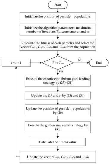
Figure 1. Flow chart for the proposed IEO algorithm.

3.2.5. Analysis of Time Complexity of Improved Algorithm

Time complexity is a key indicator to test the efficiency of an algorithm. In the EO algorithm, it is assumed that the population size is N, the search space dimension is d, the parameter initialization time is $t_1$, the time for generating random numbers is $t_2$, the time for finding the fitness is f(d), the fitness values are sorted and The time for constructing the balance pool is $t_3$, the time for updating the parameter t is $t_4$, and the time for updating the population position is $t_5$, then the total time complexity of the standard EO algorithm is as follows:

$$O(t_1+t_4+N(d{t}_2+f(d)+t_3+t_5))=O(d+f(d))$$

(39)

In the improved IEO algorithm, the time for parameter initialization and fitness calculation is the same as in the standard EO algorithm. In the iterative process, the time for introducing the leading stage of the chaotic balance pool is $t_6$, and the time for updating the improved control parameter GCP is $t_7$, the time of the golden differential mutation stage is $t_8$, then the total time complexity of IEO is as follows:

$$O(t_1+t_4+N(d{t}_2+f(d)+t_3+t_5+t_6+t_7+t_8))=O(d+f(d))$$

(40)

Based on the above analysis, the time complexity of the IEO algorithm proposed in this paper and the standard EO algorithm are in the same order of magnitude, indicating that the final time complexity of the IEO algorithm has not improved.

4. The Simulation Results

In this section, test functions are used to evaluate the performance of the proposed IEO. The experiments are carried out on 16 standard benchmark functions [29] such as continuous unimodal test functions (F1–F7), complex multimodal test functions (F8–F12), and fixed low-dimensional test functions (F13–F16). The detailed description and related information are shown in Table 1. To ensure fairness of the comparison between algorithms, the basic parameters of the algorithms are set to the same value, including the population size N = 30, the maximum number of iterations $T_{\mathit{max}}$ = 500, and the test function dimension dim = 30/100/500. The internal parameters of each basic algorithm are set as shown in Table 2. The experimental running environment is 64-bit Windows 10 operating system, the CPU is Itel Core i5-7200U, the main frequency is 2.6 GHz and the memory is 4 GB. The algorithm is written based on MATLAB R2016a. The abbreviations of the algorithm names used in this paper are shown in Table 3.

Table 1. The benchmark test functions.

Fun No.	Name	Dim	Range	Optimal Value
F1	Sphere	30/100/500	[−100, 100]	0
F2	shwefel.2.22	30/100/500	[−10, 10]	0
F3	Schwefel.1.2	30/100/500	[−100, 100]	0
F4	Schwefel.2.21	30/100/500	[−100, 100]	0
F5	Step	30/100/500	[−100, 100]	0
F6	Quartic	30/100/500	[−1.28, 1.28]	0
F7	Schwefel2.26	30/100/500	[−500, 500]	−418.9829 × dim
F8	Rastrigin	30/100/500	[−5.12, 5.12]	0
F9	Ackley	30/100/500	[−32, 32]	0
F10	Criewank	30/100/500	[−600, 600]	0
F11	Penalized 1	30/100/500	[−50, 50]	0
F12	Apline	30/100/500	[−10, 10]	0
F13	Kowalik	4	[−5, 5]	0.0003
F14	Sheke_1	4	[0, 10]	−10.1532
F15	Sheke_2	4	[0, 10]	−10.4028
F16	Shekel_3	4	[0, 10]	−10.5363

Table 2. Algorithm parameter setting.

Algorithm	Parameter
SCA [30]	M = 2;
ChOA [31]	fmax = 2.5, fmin = 0;
SSA [32]	/
MA [33]	G = 0.8, gdamp = 1, a1 = 1, a2 = 1.5, a3 = 1.5, dance = 5;
PSO [34]	vmax = 6, vmin = −6, wmax = 0.9, wmin = 0.6, c1 = c2 = 2;
GWO [35]	amax = 2, amin = 0;
WOA [36]	amax = 2, amin = 0, b = 1;
EO [23]	a1 = 2, a2 = 1, GP = 0.5;
IEO	a1 = 2, a2 = 1;

Table 3. Abbreviation of algorithm name.

Algorithm	Algorithm Description
SCA	Sine–Cosine Algorithm
ChOA	Chimp Optimization Algorithm
SSA	Salp Swarm Algorithm
MA	Mayfly Algorithm
PSO	particle swarm optimization
GWO	Gray Wolf Optimization Algorithm
WOA	Whale Optimization Algorithm
AOA	Arithmetic Optimization Algorithm
EO	Equilibrium Optimizer
m-EO	Modified Equilibrium Optimizer
AEO	Adaptive Equilibrium Optimizer
OB-L-EO	Opposition-Based Laplacian Equilibrium Optimizer
HEO	High Equilibrium Optimizer
MPA	Marine Predator Algorithm
SMA	Slime Mould Algorithm
MSCA	Modified Sine–Cosine Algorithm
GOA	Grasshopper Optimization Algorithm
MVO	Multi-Verse Optimization
IPSO	Improved Particle Swarm Optimization
HHO	Harris Hawks Optimization
BHBO	Black-Hole-Based Optimization
MOHS	Multi-Objective Harmony Search Algorithm
DE	Differential Evolution
FEA	Faster Evolutionary Algorithm
MOJA	Multi-Objective Jaye Algorithm
TLBO	Teaching–Learning-Based Optimization
MOBSA	Multi-Objective Backtracking Search Algorithm

4.1. Comparative Analysis of Algorithm Performance

To verify the overall performance of the IEO algorithm, eight algorithms are selected for comparison, including the basic EO, SCA, MA, PSO, GWO, WOA, ChOA, and SSA. To avoid performance comparison errors caused by the randomness of the algorithms, each test function is run 30 times independently, and the mean and standard deviation (Std) are used to judge the performance of the corresponding optimization algorithm. The average value reflects the convergence speed of the algorithm, and the standard deviation reflects the stability of the algorithm. The comparison results are shown in Table 4.

Table 4. Comparison of the optimal results of the benchmark function.

Fun No.	Index	SCA	ChOA	SSA	MA	PSO	GWO	WOA	EO	IEO
F1	Mean	2.46 × 101	4.71 × 10−6	2.23 × 10−7	1.67 × 10−5	2.66	2.65 × 10−27	3.36 × 10−72	4.09 × 10−41	0
	Std	6.76 × 101	7.25 × 10−6	4.00 × 10−7	4.73 × 10−5	1.21	4.47 × 10−27	1.81 × 10−71	7.73 × 10−41	0
F2	Mean	1.83 × 10−2	3.28 × 10−5	2.06	6.85 × 10−4	4.44	1.23 × 10−16	4.82 × 10−52	6.04 × 10−24	0
	Std	2.25 × 10−2	4.14 × 10−5	1.54	1.73 × 10−3	1.25	9.51 × 10−17	1.24 × 10−51	7.21 × 10−24	0
F3	Mean	1.02 × 104	1.96 × 102	1.45 × 103	5.53 × 103	2.00 × 102	1.05 × 10−5	4.33 × 104	8.54 × 10−9	0
	Std	6.28 × 103	4.00 × 102	8.12 × 102	1.30 × 102	6.03 × 101	2.32 × 10−5	1.73 × 104	3.64 × 10−8	0
F4	Mean	3.54 × 101	3.06 × 10−1	9.72	4.51 × 101	2.02	7.53 × 10−7	4.36 × 101	1.23 × 10−10	0
	Std	1.24 × 101	2.45 × 10−1	2.18	2.21 × 10−1	2.50 × 10−1	7.96 × 10−7	2.83 × 101	1.34 × 10−10	0
F5	Mean	1.43 × 101	3.70	1.74 × 10−6	1.19 × 10−5	2.53	8.01 × 10−1	4.07 × 10−1	8.97 × 10−6	5.48 × 10−7
	Std	1.31 × 101	4.38 × 10−1	2.18 × 10−6	2.22 × 10−5	1.00	3.76 × 10−1	2.14 × 10−1	6.48 × 10−6	1.12 × 10−6
F6	Mean	7.04 × 10−2	2.73 × 10−3	1.72 × 10−1	2.54 × 10−2	1.60 × 101	1.91 × 10−3	3.27 × 10−3	1.34 × 10−3	1.02 × 10−5
	Std	7.33 × 10−2	1.97 × 10−3	8.20 × 10−2	8.93 × 103	1.50 × 101	1.02 × 10−3	4.12 × 10−3	8.36 × 10−4	1.26 × 10−5
F7	Mean	−3.72 × 103	−5.71 × 103	−7.53 × 103	−9.87 × 103	−6.59 × 10−3	−6.13 × 103	−1.06 × 104	−8.84 × 103	−1.24 × 104
	Std	2.96 × 102	6.18 × 102	6.39 × 102	4.99 × 102	1.26 × 103	8.72 × 102	1.92 × 103	7.10 × 102	2.82 × 102
F8	Mean	4.65 × 101	1.17 × 101	5.69 × 101	5.13 × 101	1.68 × 102	3.45	3.79 × 10−15	1.89 × 10−15	0
	Std	4.79 × 101	1.19 × 101	1.71 × 101	2.06 × 101	3.24 × 101	3.51	1.44 × 10−14	1.03 × 10−14	0
F9	Mean	1.69 × 101	2.00 × 101	2.85	1.73	2.57	1.04 × 10−13	4.44 × 10−15	8.59 × 10−15	8.88 × 10−16
	Std	7.33	3.15 × 10−2	8.67 × 10−1	5.35 × 10−1	5.33 × 10−1	1.58 × 10−14	2.29 × 10−15	2.30 × 10−15	0
F10	Mean	1.08	2.05 × 10−2	1.93 × 10−2	2.49 × 10−2	1.24 × 10−1	9.72 × 10−4	1.32 × 10−2	3.29 × 10−4	0
	Std	5.57 × 10−1	3.45 × 10−2	1.38 × 10−2	2.98 × 10−2	4.65 × 10−2	3.83 × 10−3	4.25 × 10−2	1.80 × 10−3	0
F11	Mean	1.44 × 104	4.69 × 10−1	7.16	5.20 × 10−1	4.04 × 10−2	4.89 × 10−2	2.27 × 10−2	4.60 × 10−7	2.35 × 10−8
	Std	5.90 × 104	1.82 × 10−1	3.72	7.08 × 10−1	2.44 × 10−2	2.56 × 10−2	1.45 × 10−2	3.58 × 10−7	2.65 × 10−8
F12	Mean	1.54	4.06 × 10−3	4.07	2.19 × 10−4	6.01	7.29 × 10−4	2.16 × 10−39	2.73 × 10−24	0
	Std	3.19	1.24 × 10−2	2.22	4.02 × 10−4	2.90	7.62 × 10−4	1.18 × 10−38	4.45 × 10−24	0
F13	Mean	9.79 × 10−4	9.79 × 10−4	1.33 × 10−3	3.08 × 10−3	8.97 × 10−4	9.73 × 10−3	6.49 × 10−4	2.35 × 10−3	3.56 × 10−4
	Std	3.24 × 10−4	3.24 × 10−4	5.16 × 10−4	6.91 × 10−3	1.30 × 10−4	1.31 × 10−2	4.45 × 10−4	6.11 × 10−3	8.45 × 10−5
F14	Mean	−2.6931	−1.6733	−7.8901	−5.9683	−8.0397	−9.3935	−8.2692	−8.1255	−10.1532
	Std	1.9152	1.6798	3.112	3.5485	2.739	2.0068	2.7214	2.77	5.79 × 10−15
F15	Mean	−4.0105	−3.6312	−9.1095	−6.6698	−8.9849	−10.2252	−8.2252	−9.3623	−10.4028
	Std	1.6975	1.9582	2.6852	3.8057	2.9115	0.97032	3.1739	2.4134	1.04 × 10−15
F16	Mean	−4.7637	−4.4468	−8.0623	−7.8211	−9.5646	−9.9948	−7.1163	−9.682	−10.5363
	Std	2.2925	1.6923	3.3784	3.6619	2.2428	2.0586	3.5352	2.2541	2.06 × 10−15

As seen from Table 4, for the continuous unimodal test functions F1~F4, the IEO can locate its theoretical optimal value and the standard deviation is 0, which proves that the algorithm has excellent stability. For functions F5 and F6, although the theoretical optimal value has not been found, the average value and stability are superior to those of the other eight algorithms. IEO can also obtain high-precision solutions for complex multimodal test functions. Especially for functions F8, F10, and F12, the IEO has successfully located the theoretical optimal value. For functions F7, F9, and F11, although IEO could not locate the theoretical optimal value, the solution accuracy was better than that of the other eight algorithms, which proves that IEO has a superior ability to escape the local extreme value. For the fixed low-dimensional test functions (except for F13), the IEO algorithm can also locate the theoretical optimal value.

4.2. Convergence Analysis

To intuitively compare the optimization performance of the proposed algorithm with other algorithms, the advantages of the IEO algorithm will be highlighted. Figure 2 shows the average convergence curve of partial benchmark functions, where the abscissa represents the number of iterations, and the ordinate represents the logarithm of the average optimal value of the function. As seen from Figure 2, the convergence accuracy of the IEO algorithm is significantly higher than other algorithms, indicating that the golden sine strategy can effectively improve the problem of the candidate solution relying too much on the equalization pool. Figure 2a−f show the convergence curves of the single-peak and the multi-peak test functions. Figure 2 show that the convergence speed of the IEO algorithm is significantly faster than that of the other algorithms. It is worth noting that functions F1, F2, F3, and F12 can quickly converge to the theoretical optimal value under the same number of iterations. This indicates that the chaotic equilibrium pool leading strategy corrects the blind movement direction of the population and avoids ineffective searches. Figure 2g,h are the fixed multi-peak test functions. It can be seen from these figures that the number of stagnations of the IEO algorithm is significantly less than that of other algorithms. Even if it falls into a local extremum for a short time, it can quickly jump out of the local extremum. The improved nonlinear dynamic generation mechanism can effectively balance global search and local exploitation. Based on the above analysis, the IEO algorithm has higher solution accuracy and convergence speed than other algorithms, proving its effectiveness and superiority.

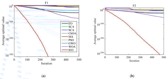
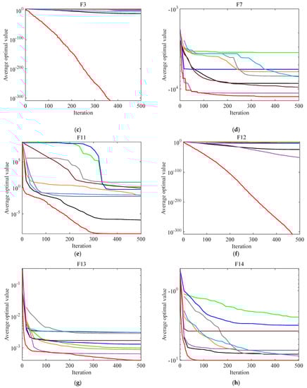
Figure 2. Partial convergence curves of the proposed IEO and other metaheuristic algorithms on the benchmark test functions: (a) Convergence curve of F1; (b) Convergence curve of F2; (c) Convergence curve of F3; (d) Convergence curve of F7; (e) Convergence curve of F11; (f) Convergence curve of F12; (g) Convergence curve of F13; (h) Convergence curve of F14.

4.3. Comparison with Other Improved EO Algorithms

To highlight the competitiveness of the proposed algorithm, the proposed EO algorithm is compared with the latest improved EO algorithm, including m-EO [37], AEO [38], OB-L-EO [39], and HEO [40]. To achieve fairness of the comparison, the number of iterations of all algorithms is 500, the population size is 30, the search dimensions of each function (except for the fixed low-dimensional test functions F13~F16) are 30/100/500, and each algorithm is run 30 times independently. The comparison results are shown in Table 5 and Table 6, where “-” represents missing data in the literature.

Table 5. Results of comparison with other improved algorithms in different dimensions.

Fun No.	Dim	m-EO [37]		AEO [38]		OB-L-EO [39]		HEO [40]		IEO
		Mean	Std	Mean	Std	Mean	Std	Mean	Std	Mean	Std
	30	0	0	1.62 × 10−104	7.47 × 10−104	6.76 × 10−212	0	5.60 × 10−196	0	0	0
F1	100	1.53 × 10−304	0	1.47 × 10−97	4.93 × 10−97	0	0	-	-	0	0
	500	0	0	3.56 × 10−78	1.48 × 10−77	-	-	-	-	0	0
	30	3.93 × 10−167	0	1.38 × 10−56	3.65 × 10−56	1.93 × 10−108	8.00 × 10−108	0	2.75 × 10−94	0	0
F2	100	3.09 × 10−161	1.58 × 10−160	1.99 × 10−52	3.36 × 10−52	0	0	-	-	0	0
	500	1.36 × 10−160	5.90 × 10−160	3.70 × 10−43	9.08 × 10−43	-	-	-	-	0	0
	30	2.71 × 10−306	0	4.24 × 10−38	2.30 × 10−37	6.93 × 10−187	0	6.44 × 10−198	3.09 × 10−106	0	0
F3	100	8.50 × 10−297	0	4.01 × 10−9	1.99 × 10−8	0	0	-	-	0	0
	500	4.63 × 10−293	0	2.64 × 102	7.78 × 102	-	-	-	-	0	0
	30	2.31 × 10−159	1.17 × 10−158	1.94 × 10−46	9.14 × 10−46	4.73 × 10−103	1.60 × 10−102	1.22 × 10−96	2.02 × 10−95	0	0
F4	100	2.83 × 10−157	9.04 × 10−157	4.53 × 10−42	1.42 × 10−41	0	0	-	-	1.52 × 10−314	0
	500	1.48 × 10−154	7.46 × 10−154	5.05 × 10−28	2.35 × 10−27	-	-	-	-	7.39 × 10−307	0
	30	9.23 × 10−5	4.18 × 10−5	6.45 × 10−6	4.98 × 10−6	9.09 × 10−5	5.98 × 10−5	1.11 × 10−3	1.34 × 10−3	5.48 × 10−7	1.12 × 10−6
F5	100	5.28 × 10−3	4.24 × 10−3	3.49	7.01 × 10−1	1.53 × 10−1	2.05 × 10−1	-	-	9.17 × 10−4	4.50 × 10−4
	500	4.92 × 10−2	5.50 × 10−2	8.99 × 101	2.30 × 10−3	-	-	-	-	3.46 × 10−3	1.91 × 10−3
	30	2.47 × 10−4	2.23 × 10−4	1.10 × 10−3	5.87 × 10−4	4.70 × 10−4	3.05 × 10−4	1.18 × 10−5	7.32 × 10−5	1.02 × 10−5	1.26 × 10−5
F6	100	3.47 × 10−4	2.50 × 10−4	2.30 × 10−3	8.46 × 10−4	1.47 × 10−4	1.22 × 10−4	-	-	1.25 × 10−4	1.12 × 10−4
	500	5.11 × 10−4	3.90 × 10−4	4.80 × 10−3	2.30 × 10−3	-	-	-	-	2.02 × 10−4	1.66 × 10−4
	30	−1.22 × 104	1.02 × 103	−8.91 × 103	6.21 × 102	−9.06 × 103	9.28 × 102	-	-	−1.24 × 104	2.82 × 102
F7	100	−4.19 × 104	9.63	−2.58 × 104	1.34 × 103	−2.85 × 104	2.09 × 103	-	-	−4.19 × 104	1.63
	500	−2.09 × 105	1.87 × 102	−7.62 × 104	5.92 × 103	-	-	-	-	−1.96 × 105	1.13 × 102
	30	0	0	0	0	0	0	0	0	0	0
F8	100	0	0	0	0	0	0	-	-	0	0
	500	0	0	0	0	-	-	-	-	0	0
	30	8.88 × 10−16	0	5.98 × 10−15	1.79 × 10−15	8.88 × 10−16	4.01 × 10−31	8.88 × 10−16	0	8.88 × 10−16	0
F9	100	8.88 × 10−16	0	6.81 × 10−15	1.70 × 10−15	8.88 × 10−16	8.88 × 10−16	-	-	8.88 × 10−16	0
	500	8.88 × 10−16	0	7.52 × 10−15	2.03 × 10−15	-	-	-	-	8.88 × 10−16	0
	30	0	0	0	0	0	0	0	0	0	0
F10	100	0	0	0	0	0	0	-	-	0	0
	500	0	0	0	0	-	-	-	-	0	0
	30	6.26 × 10−6	3.92 × 10−6	5.22 × 10−7	5.00 × 10−7	6.29 × 10−6	4.35 × 10−6	1.79 × 10−5	5.06 × 10−5	2.35 × 10−8	2.65 × 10−8
F11	100	2.18 × 10−5	1.78 × 10−5	3.45 × 10−2	8.20 × 10−3	5.83 × 10−4	1.14 × 10−3	-	-	8.00 × 10−3	3.54 × 10−3
	500	1.98 × 10−5	2.25 × 10−5	6.44 × 10−1	3.48 × 10−2	-	-	-	-	9.75 × 10−2	1.75 × 10−2
	30	1.65 × 10−165	0	-	-	-	-	-	-	0	0
F12	100	1.65 × 10−164	0	-	-	-	-	-	-	0	0
	500	5.61 × 10−160	0	-	-	-	-	-	-	0	0

Table 6. Results of comparison with other improved algorithms under fixed low dimension (dim = 4).

Fun No.	m-EO [37]		AEO [38]		OB-L-EO [39]		HEO [40]		IEO
	Mean	Std	Mean	Std	Mean	Std	Mean	Std	Mean	Std
F13	1.55 × 10−1	4.93 × 10−1	1.10 × 10−2	3.70 × 10−3	4.61 × 10−4	3.47 × 10−4	1.02	3.87	3.56 × 10−4	8.45 × 10−5
F14	−9.33	2.23	−8.45	2.44	−1.02 × 101	9.12 × 10−6	-	-	−1.02 × 101	5.79 × 10−15
F15	−1.01 × 101	1.35	−9.47	2.13	−1.04 × 101	7.99 × 10−6	-	-	−1.04 × 101	1.04 × 10−15
F16	−1.03 × 101	9.87 × 10−1	−9.82	1.87	−1.02 × 101	1.36	-	-	−1.05 × 101	2.06 × 10−15

As seen from Table 5 and Table 6, for single-peak functions F1~F3, IEO can effectively obtain the theoretical optimal value when solving functions with 30, 100 and 500 dimensions, while the other four algorithms have decreased accuracy and stability with increasing dimensions. For function F4, although IEO is slightly inferior to the OB-L-EO algorithm in the case of 100 dimensions, IEO is better than the other four algorithms in 30 and 500 dimensions. For functions F5 and F6, IEO is superior to the other four algorithms in all dimensions, although it fails to obtain the theoretical optimal value. For the F7 function, although the solution accuracy of IEO in 500 dimensions is slightly inferior to that of m-EO, the standard deviation is better than that of m-EO and the other three algorithms. For function F11, IEO is slightly inferior to m-EO in 100 and 500 dimensions, which shows that IEO still needs to be improved in performance when solving high-dimensional multimodal optimization problems. It is worth mentioning that for functions F12~F16, IEO still has excellent solution accuracy and stability, while the four algorithms have low solution accuracy and poor stability. Therefore, it can be concluded that the performance of the IEO algorithm has more significant advantages compared with the improved m-EO, AEO, OB-L-EO, E-SFDBEO, and HEO.

4.4. Wilcoxon Rank Sum Test

In the simulations described above, the experimental results are not compared independently each time. To reflect the performance of the algorithm more comprehensively, this paper uses the Wilcoxon rank sum test, verifying whether the results of each run of IEO are statistically significantly different from those of the other algorithms. The rank sum test is carried out at the significance level of p = 5%. If the p value is less than 5%, the H0 hypothesis is rejected, which indicates that the two comparison algorithms are significantly different. Otherwise, the H0 hypothesis is accepted, which indicates that the optimization results of the two algorithms are the same [41].

Table 7 presents the rank sum test p values of IEO and the other algorithms including SCA, ChOA, SSA, MA, PSO, GWO, WOA, and EO, on the 16 test functions. In the table, “R” represents the significance judgement result, and the symbols “+”, “=”, and “−” represent that the rank and statistical results of the IEO algorithm, being superior, equal and inferior to the other algorithms, respectively. As seen from Table 7, all p values are much less than 5%, which indicates that there is a significant difference between the IEO algorithm and the other eight algorithms, and IEO is significantly excellent.

Table 7. Wilcoxon rank sum test results.

Fun No.	SCA	ChOA	SSA	MA	PSO	GWO	WOS	EO
	p Value R	p Value R	p Value R	p Value R	p Value R	p Value R	p Value R	p Value R
F1	3.31 × 10−20 +	3.31 × 10−20 +	3.31 × 10−20 +	3.31 × 10−20 +	3.31 × 10−20 +	3.31 × 10−20 +	3.31 × 10−20+	3.31 × 10−20 +
F2	3.31 × 10−20 +	3.31 × 10−20 +	3.31 × 10−20 +	3.31 × 10−20 +	3.31 × 10−20 +	3.31 × 10−20 +	3.31 × 10−20 +	3.31 × 10−20 +
F3	3.31 × 10−20 +	3.31 × 10−20 +	3.31 × 10−20 +	3.31 × 10−20 +	3.31 × 10−20 +	3.31 × 10−20 +	3.31 × 10−20 +	3.31 × 10−20 +
F4	3.31 × 10−20 +	3.31 × 10−20 +	3.31 × 10−20 +	3.31 × 10−20 +	3.31 × 10−20 +	3.31 × 10−20 +	3.31 × 10−20 +	3.31 × 10−20 +
F5	7.07 × 10−18 +	7.07 × 10−18 +	1.11 × 10−2 +	3.26 × 10−13 +	7.07 × 10−18 +	7.07 × 10−18 +	7.07 × 10−18 +	7.49 × 10−16 +
F6	7.07 × 10−18 +	8.19 × 10−12 +	7.07 × 10−18 +	7.07 × 10−18 +	7.07 × 10−18 +	1.01 × 10−17 +	1.17 × 10−15 +	1.43 × 10−16 +
F7	7.07 × 10−18 +	7.07 × 10−18 +	7.07 × 10−18 +	7.07 × 10−18 +	7.07 × 10−18 +	7.07 × 10−18 +	2.44 × 10−11 +	3.15 × 10−12 +
F8	3.31 × 10−20 +	3.31 × 10−20 +	3.31 × 10−20 +	3.31 × 10−20 +	3.31 × 10−20 +	3.31 × 10−20 +	6.50 × 10−3 +	1.23 × 10−2 +
F9	3.31 × 10−20 +	3.31 × 10−20 +	3.31 × 10−20 +	3.31 × 10−20 +	3.31 × 10−20 +	2.85 × 10−20 +	1.54 × 10−11 +	1.03 × 10−22 +
F10	3.31 × 10−20 +	3.31 × 10−20 +	3.31 × 10−20 +	3.31 × 10−20 +	3.31 × 10−20 +	6.25 × 10−21 +	1.80 × 10−3 +	2.30 × 10−2 +
F11	7.07 × 10−18 +	3.21 × 10−17 +	7.07 × 10−18 +	7.07 × 10−18 +	7.07 × 10−18 +	7.07 × 10−18 +	7.07 × 10−18 +	1.60 × 10−16 +
F12	3.31 × 10−20 +	3.31 × 10−20 +	3.31 × 10−20 +	3.31 × 10−20 +	3.31 × 10−20 +	3.31 × 10−20 +	3.31 × 10−20 +	3.31 × 10−20 +
F13	3.23 × 10−17 +	7.07 × 10−18 +	2.07 × 10−17 +	1.26 × 10−6 +	1.21 × 10−17 +	6.10 × 10−3 +	8.59 × 10−12 +	1.55 × 10−8 +
F14	3.31 × 10−20 +	3.31 × 10−20 +	3.75 × 10−7 +	3.68 × 10−10 +	3.31 × 10−20 +	3.31 × 10−20 +	3.31 × 10−20 +	1.89 × 10−20 +
F15	3.31 × 10−20 +	3.31 × 10−20 +	3.69 × 10−6 +	2.57 × 10−20 +	1.76 × 10−6 +	3.31 × 10−20 +	3.31 × 10−20 +	4.38 × 10−21 +
F16	3.31 × 10−20 +	3.31 × 10−20 +	3.23 × 10−5 +	1.32 × 10−20 +	3.80 × 10−7 +	3.31 × 10−20 +	3.31 × 10−20 +	1.76 × 10−20 +
+/=/−	16/0/0	16/0/0	16/0/0	16/0/0	16/0/0	16/0/0	16/0/0	16/0/0

+ in the table indicates that the ranking and statistical results of the IEO algorithm are better than other algorithms.

4.5. Experimental Analysis of CEC2014 Test Function

Most of the CEC2014 test functions [42] are composed of the weights of multiple basic optimization test functions, making the characteristics of the test functions more complex. In this paper, the proposed IEO is tested against these complex test functions. On the one hand, these functions can effectively reflect the superior performance of IEO for complex function optimization. On the other hand, the combinatorial optimization of multiple test functions reflects the applicability of IEO to different complex optimization problems. Therefore, to further test the performance of IEO, this paper selects the CEC2014 single-objective optimization function for solution analysis, including unimodal, multimodal, Hybrid and composition type functions. Table 8 shows the relevant information of CEC2014 functions. This study compares IEO with eight algorithms including SCA, ChOA, SSA, GWO, WOA, AOA, PSO and EO. To ensure fairness of the algorithm comparison, the population size N = 30, the maximum iterations $T_{\mathit{max}}$ = 1000, the dimension dim = 30, is set to the same values in each algorithm, which is run 30 times independently, and the mean and standard deviation are recorded. The results are shown in Table 9.

Table 8. CEC2014 test function.

Fun No.	Function type	Function Name	Optimal Value
CEC01	Unimodal Function	Rotated High Conditioned Elliptic Function	100
CEC02		Rotated Bent Cigar Function	200
CEC03		Rotated Discus Function	300
CEC04	Multimodal Function	Shifted and Rotated Rosenbrock’s Function	400
CEC05		Shifted and Rotated Ackley’s Function	500
CEC06		Shifted and Rotated Weierstrass Function	600
CEC07		Shifted and Rotated Griewank’s Function	700
CEC08		Shifted Rastrigin’s Function	800
CEC09		Shifted and Rotated Rastrigin’s Function	900
CEC10		Shifted Schwefel’s Function	1000
CEC11		Shifted and Rotated Schwefel’s Function	1100
CEC12		Shifted and Rotated Katsuura Function	1200
CEC13		Shifted and Rotated HappyCat Function	1300
CEC14		Shifted and Rotated HGBat Function	1400
CEC15		Shifted and Rotated Expanded Griewank’s plus Rosenbrock’s Function	1500
CEC16		Shifted and Rotated Expanded Scaffer’s F6 Function	1600
CEC17	Hybrid Function	Hybrid Function 1 (N = 3)	1700
CEC18		Hybrid Function 2 (N = 3)	1800
CEC19		Hybrid Function 3 (N = 4)	1900
CEC20		Hybrid Function 4 (N = 4)	2000
CEC21		Hybrid Function 5 (N = 5)	2100
CEC22		Hybrid Function 6 (N = 5)	2200
CEC23	Composition Function	Composition Function 1 (N = 5)	2300
CEC24		Composition Function 2 (N = 3)	2400
CEC25		Composition Function 3 (N = 3)	2500
CEC26		Composition Function 4 (N = 5)	2600
CEC27		Composition Function 5 (N = 5)	2700
CEC28		Composition Function 6 (N = 5)	2800
CEC29		Composition Function 7 (N = 3)	2900
CEC30		Composition Function 8 (N = 3)	3000

Table 9. CEC2014 function optimization comparison.

Fun No.	Index	SCA	ChOA	SSA	GWO	WOA	AOA	PSO	EO	IEO
CEC01	Mean	4.193 × 108	5.988 × 108	2.376 × 107	8.936 × 107	8.553 × 107	1.362 × 109	7.423 × 106	7.740 × 106	5.473 × 106
	Std	1.085 × 108	1.080 × 108	1.168 × 107	6.043 × 107	5.417 × 107	3.235 × 108	3.835 × 106	3.691 × 106	3.216 × 106
CEC02	Mean	2.651 × 1010	4.381 × 1010	1.302 × 104	2.464 × 109	3.427 × 109	7.125 × 1010	4.245 × 105	2.111 × 104	2.862 × 103
	Std	4.297 × 109	6.867 × 109	1.066 × 104	2.541 × 109	3.135 × 109	1.117 × 1010	2.267 × 105	1.195 × 104	5.698 × 103
CEC03	Mean	5.876 × 104	8.265 × 104	7.365 × 104	4.529 × 104	4.585 × 104	8.101 × 104	1.267 × 104	8.549 × 103	3.657 × 103
	Std	1.192 × 104	8.024 × 103	1.941 × 104	1.216 × 104	1.056 × 104	8.235 × 103	8.234 × 104	4.531 × 103	2.577 × 103
CEC04	Mean	2.547 × 103	3.335 × 103	5.315 × 102	6.967 × 102	6.616 × 102	1.226 × 104	5.168 × 102	5.129 × 102	5.074 × 102
	Std	7.605 × 102	1.430 × 103	4.515 × 101	1.216 × 102	5.316 × 101	3.527 × 103	2.935 × 101	3.320 × 101	2.681 × 101
CEC05	Mean	5.211 × 102	5.211 × 102	5.201 × 102	5.210 × 102	5.211 × 102	5.209 × 102	5.209 × 102	5.209 × 102	5.207 × 102
	Std	5.832 × 10−2	5.332 × 10−2	9.926 × 10−2	5.761 × 10−2	5.325 × 10−2	6.787 × 10−2	9.917 × 10−2	1.260 × 10−1	4.640 × 10−2
CEC06	Mean	6.365 × 102	6.364 × 102	6.232 × 102	6.163 × 102	6.157 × 102	6.392 × 102	6.207 × 102	6.105 × 102	6.098 × 102
	Std	2.705	2.021	3.635	3.113	2.646	1.982	3.647	3.226	1.081
CEC07	Mean	9.172 × 102	1.178 × 103	7.021 × 102	7.226 × 102	7.231 × 102	1.352 × 103	7.006 × 102	7.001 × 102	7.000 × 102
	Std	3.107 × 101	8.536 × 101	1.456 × 10−2	1.897 × 101	1.949 × 101	1.113 × 101	1.663 × 10−1	1.543 × 10−2	1.384 × 10−2
CEC08	Mean	1.073 × 103	1.067 × 103	9.572 × 102	8.878 × 102	8.892 × 102	1.151 × 103	9.242 × 102	8.614 × 102	8.552 × 102
	Std	2.538 × 101	2.213 × 101	4.215 × 101	2.445 × 101	2.088 × 101	3.074 × 101	2.338 × 101	1.554 × 101	1.213 × 101
CEC09	Mean	1.205 × 103	1.187 × 103	1.062 × 103	1.005 × 103	1.023 × 103	1.219 × 103	1.045 × 103	9.883 × 102	9.680 × 102
	Std	2.349 × 101	2.147 × 101	4.244 × 101	2.038 × 101	3.805 × 101	2.791 × 101	2.769 × 101	2.784 × 101	1.960 × 101
CEC10	Mean	7.670 × 103	7.801 × 103	4.780 × 103	3.595 × 103	3.564 × 103	7.274 × 103	4.258 × 103	2.873 × 103	2.814 × 103
	Std	4.632 × 102	9.379 × 102	7.847 × 102	7.425 × 102	5.144 × 102	6.115 × 102	4.678 × 102	6.086 × 102	4.535 × 102
CEC11	Mean	8.682 × 103	8.937 × 103	5.050 × 103	4.265 × 103	4.481 × 103	7.717 × 103	4.505 × 103	5.093 × 103	4.862 × 103
	Std	3.155 × 102	2.901 × 102	7.846 × 102	6.525 × 102	1.219 × 103	5.136 × 102	5.789 × 102	7.821 × 102	8.284 × 102
CEC12	Mean	1.203 × 103	1.203 × 103	1.201 × 103	1.202 × 103	1.203 × 103	1.202 × 103	1.202 × 103	1.202 × 103	1.201 × 103
	Std	3.934 × 10−1	4.052 × 10−1	4.315 × 10−1	1.214	1.104	4.557 × 10−1	6.887 × 10−1	3.582 × 10−1	3.486 × 10−1
CEC13	Mean	1.304 × 103	1.304 × 103	1.301 × 103	1.301 × 103	1.301 × 103	1.307 × 103	1.301 × 103	1.300 × 103	1.300 × 103
	Std	2.691 × 10−1	5.682 × 10−1	1.538 × 10−1	3.385 × 10−1	5.589 × 10−1	9.561 × 10−1	1.316 × 10−1	9.216 × 10−2	7.381 × 10−2
CEC14	Mean	1.474 × 103	1.556 × 103	1.401 × 103	1.407 × 103	1.407 × 103	1.639 × 103	1.401 × 103	1.400 × 103	1.400 × 103
	Std	1.115 × 101	3.481 × 101	2.232 × 10−1	8.419	9.241	3.676 × 101	1.764 × 10−1	1.406 × 10−1	1.226 × 10−1
CEC15	Mean	1.854 × 104	1.258 × 105	1.514 × 103	1.799 × 103	1.800 × 103	2.964 × 105	1.515 × 103	1.509 × 103	1.508 × 103
	Std	1.139 × 104	9.523 × 104	4.705	5.662 × 102	7.871 × 102	1.126 × 105	2.048	3.235	2.926
CEC16	Mean	1.613 × 103	1.613 × 103	1.613 × 103	1.612 × 103	1.612 × 103	1.613 × 103	1.613 × 103	1.612 × 103	1.611 × 103
	Std	2.372 × 10−1	2.239 × 10−1	7.115 × 10−1	6.959 × 10−1	7.963 × 10−1	3.641 × 10−1	4.339 × 10−1	6.615 × 10−1	1.373 × 10−1
CEC17	Mean	1.385 × 107	3.290 × 107	1.265 × 106	2.747 × 106	2.720 × 106	8.805 × 107	6.051 × 105	8.126 × 105	5.846 × 105
	Std	7.717 × 106	1.947 × 107	8.693 × 105	2.881 × 106	2.547 × 106	3.984 × 107	5.482 × 105	8.573 × 105	4.147 × 105
CEC18	Mean	3.134 × 108	9.120 × 108	1.094 × 104	2.202 × 107	1.692 × 107	2.339 × 109	4.065 × 103	4.932 × 103	3.767 × 103
	Std	1.335 × 108	9.997 × 108	7.508 × 103	4.057 × 107	2.724 × 107	1.625 × 109	2.656 × 103	3.687 × 103	2.333 × 103
CEC19	Mean	2.033 × 103	2.163 × 103	1.920 × 103	1.950 × 103	1.970 × 103	2.250 × 103	1.915 × 103	1.912 × 103	1.909 × 103
	Std	3.652 × 101	1.070 × 102	1.780 × 101	3.450 × 101	4.450 × 101	1.155 × 102	3.201	1.511 × 101	2.194
CEC20	Mean	4.452 × 104	1.084 × 105	3.280 × 104	3.057 × 104	2.486 × 104	2.205 × 105	1.761 × 104	1.460 × 104	1.246 × 104
	Std	2.328 × 104	3.923 × 104	1.675 × 104	1.265 × 104	6.620 × 104	8.616 × 104	6.945 × 103	5.620 × 103	4.175 × 103
CEC21	Mean	4.066 × 106	1.130 × 107	4.137 × 105	8.915 × 105	1.334 × 106	2.428 × 107	3.351 × 105	4.266 × 105	3.056 × 105
	Std	2.341 × 106	3.245 × 106	3.892 × 105	2.086 × 106	2.125 × 106	2.126 × 107	2.665 × 105	4.378 × 105	2.319 × 105
CEC22	Mean	3.260 × 103	3.177 × 103	2.794 × 103	2.673 × 103	2.61 × 103	4.971 × 103	3.045 × 103	2.658 × 103	2.588 × 103
	Std	2.169 × 102	2.647 × 102	2.090 × 102	2.054 × 102	2.762 × 102	2.105 × 103	2.926 × 102	2.045 × 102	2.022 × 102
CEC23	Mean	2.716 × 103	2.745 × 103	2.639 × 103	2.641 × 103	2.644 × 103	2.511 × 103	2.614 × 103	2.616 × 103	2.615 × 103
	Std	1.951 × 101	4.447 × 101	1.235 × 101	1.272 × 101	1.045 × 101	6.233 × 101	4.451 × 10−2	4.481 × 10−4	7.714 × 10−2
CEC24	Mean	2.611 × 103	2.600 × 103	2.642 × 103	2.600 × 103	2.600 × 103	2.600 × 103	2.624 × 103	2.600 × 103	2.600 × 103
	Std	1.953 × 101	4.626 × 10−2	7.915	1.347 × 10−2	1.094 × 10−2	8.515 × 10−2	6.836	4.430 × 10−3	3.170 × 10−3
CEC25	Mean	2.741 × 103	2.712 × 103	2.719 × 103	2.712 × 103	2.713 × 103	2.700 × 103	2.175 × 103	2.702 × 103	2.700 × 103
	Std	1.191 × 101	1.369 × 101	6.265	4.859	5.356	0	4.658	3.651	0
CEC26	Mean	2.703 × 103	2.796 × 103	2.701 × 103	2.738 × 103	2.741 × 103	2.782 × 103	2.777 × 103	2.737 × 103	2.720 × 103
	Std	5.079 × 10−1	4.839 × 101	1.473 × 10−1	5.968 × 101	4.956 × 101	3.367 × 101	4.289 × 101	4.885 × 101	4.784 × 101
CEC27	Mean	3.864 × 103	3.923 × 103	3.573 × 103	3.377 × 103	3.384 × 103	3.832 × 103	3.560 × 103	3.384 × 103	3.309 × 103
	Std	2.728 × 102	2.002 × 102	2.062 × 102	1.288 × 102	1.498 × 102	5.433 × 102	2.390 × 102	1.113 × 102	1.030 × 102
CEC28	Mean	5.593 × 103	5.745 × 103	4.270 × 103	4.190 × 103	4.205 × 103	4.970 × 103	6.778 × 103	3.846 × 103	3.813 × 103
	Std	4.547 × 102	2.475 × 102	4.646 × 102	4.412 × 102	3.744 × 102	2.700 × 103	8.031 × 102	2.422 × 102	1.592 × 102
CEC29	Mean	3.026 × 107	5.153 × 107	4.547 × 106	3.430 × 106	1.248 × 107	3.318 × 108	4.657 × 103	2.44 × 106	1.716 × 106
	Std	1.490 × 107	3.314 × 107	7.902 × 106	7.411 × 106	8.591 × 106	2.614 × 108	1.894 × 103	4.13 × 106	3.348 × 106
CEC30	Mean	4.652 × 105	8.103 × 105	3.876 × 104	8.482 × 104	8.637 × 104	5.306 × 106	7.785 × 103	8.451 × 103	7.306 × 103
	Std	1.775 × 105	2.142 × 105	2.146 × 104	5.220 × 104	5.851 × 104	3.825 × 106	3.215 × 103	6.567 × 103	2.764 × 103

Table 9 shows that IEO has obtained good results on 25 test functions. Especially on functions CEC07, CEC13 and CEC14, the IEO basically converges to the theoretical optimal value. For function CEC05, the average value of IEO is slightly inferior to the SSA, but the standard deviation is superior to the other eight algorithms, which indicates that IEO has better stability. For functions CEC11, CEC23, CEC26 and CEC29, the solution accuracy of IEO is slightly inferior to GWO, AOA, SSA and PSO. Generally, the proposed algorithm has more prominent advantages in the CEC2014 test function compared with the other eight algorithms.

5. Application to Solve the OPF Optimization Problem

To validate the effectiveness and feasibility of the IEO algorithm in solving OPF problems, this paper was tested on a standard IEEE 30-bus test system. The IEEE 30-bus system model consists of six generator units, four transformers and nine reactive power compensation buses. The locations of the generators are at buses 1, 2, 3, 8, 11, and 13. The transformers are in lines 6–9, 6–10, 4–12, and 28–27. The reactive power compensations are at buses 10, 12, 15, 17, 20, 21, 23, 24, and 29. It is worth mentioning that the total real and reactive power of this system demand are 2.834 p.u. and 1.262 p.u., respectively, at the base MVA of 100. Figure 3 shows the single line diagram of the IEEE 30-bus system, in which bus 1 is the balance bus, buses 2, 5, 8, 11, and 13 are PV buses, and the remaining buses are PQ buses. The maximum number of experiments in this section is set to 500 iterations and the comparative analysis was carried out for each case of the selected targets. The details are described in the forthcoming subsections. The optimal settings of the controlling parameters for the proposed method are also detailed in Table 10.

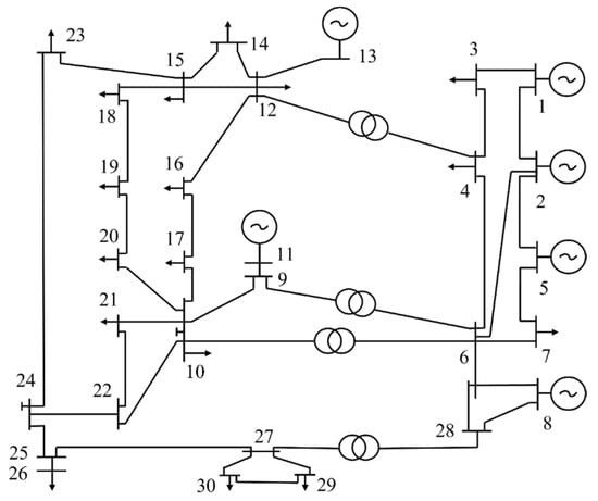
Figure 3. IEEE 30-bus system single line diagram.

Table 10. The controlling parameters of the IEEE 30-bus system for cases 1 to 3 using the IEO based optimization method.

Parameters	Selective Objective
	FC	APL	VD
Pg1 (MW)	177.0567	51.2493	176.3369
Pg2 (MW)	48.6972	80.0000	48.9664
Pg3 (MW)	21.3043	50.0000	21.6539
Pg4 (MW)	21.0814	35.0000	22.0081
Pg5 (MW)	11.8842	30.0000	12.2721
Pg6 (MW)	12.0000	40.0000	12.0000
V1 (p.u.)	1.1000	1.1000	1.0391
V2 (p.u.)	1.0879	1.0976	1.0227
V3 (p.u.)	1.0617	1.0799	1.0156
V4 (p.u.)	1.0694	1.0869	1.0051
V5 (p.u.)	1.1000	1.1000	1.0245
V6 (p.u.)	1.1000	1.1000	0.9951
T11(6–9)	1.0447	1.0546	1.0403
T12(6–10)	0.9000	0.9000	0.9000
T15(4–12)	0.9863	0.9841	0.9506
T36(28–27)	0.9657	0.9727	0.9691
QC1 (MVAR)	5.0000	5.0000	4.8490
QC2 (MVAR)	5.0000	5.0000	0.3485
QC3 (MVAR)	5.0000	4.9996	4.9997
QC4 (MVAR)	5.0000	5.0000	0.0048
QC5 (MVAR)	5.0000	4.8218	5.0000
QC6 (MVAR)	5.0000	5.0000	4.9999
QC7 (MVAR)	3.8491	3.6385	5.0000
QC8 (MVAR)	5.0000	5.0000	4.9997
QC9 (MVAR)	2.7434	2.5216	2.6104
Fuel Cost ($/h)	799.0680	999.9988	803.6371
APL (MW)	8.6245	2.8506	9.9343
VD	1.8583	2.0489	0.0944

5.1. Case 1: Fuel Cost Minimization (FC)

To verify the effectiveness of IEO in solving OPF problems, the fuel cost of each generating unit was considered for optimization as the objective function. The simulation results of the IEO for case 1 are compared with those of the marine predator algorithm (MPA) [13], slime mould algorithm (SMA) [15], modified sine–cosine algorithm (MSCA) [43], grasshopper optimization algorithm (GOA) [44], multi-verse optimization (MVO) [44], improved particle swarm optimization (IPSO) [45], and Harris hawks optimization (HHO) [46], as shown in Table 11.

Table 11. Comparison of the IEO with other algorithms for case 1.

Parameter	Fuel Cost (FC)
	IEO	EO	MPA [13]	SMA [15]	MSCA [43]	GOA [44]	MVO [44]	IPSO [45]	HHO [46]
Pg1 (MW)	177.0567	176.8497	177.032	176.2134	177.401	-	-	177.0431	176.97
Pg2 (MW)	48.6972	48.9155	48.688	48.8501	48.632	48.0194	51.189	49.209	48.88
Pg3 (MW)	21.3043	21.7782	21.305	21.5222	21.2376	20.9145	21.311	21.5135	21.42
Pg4 (MW)	21.0814	18.8509	21.081	22.1311	20.8615	20.2342	21.173	22.648	22.02
Pg5 (MW)	11.8842	13.8211	11.912	12.2063	11.9385	15.726	22.699	10.4146	12.29
Pg6 (MW)	12.0000	12.1079	12.004	12.0000	12	13.5828	16.587	12	11.21
V1 (p.u.)	1.1000	1.0998	1.100	1.0500	1.1	1.09356	1.0813	1.05	-
V2 (p.u.)	1.0879	1.0796	1.088	1.0381	1.0867	1.040936	1.0689	1.0462	-
V3 (p.u.)	1.0617	1.0345	1.062	1.0110	1.0604	0.969193	1.0406	1.0459	-
V4 (p.u.)	1.0694	1.0452	1.069	1.0194	1.0923	0.987262	1.0442	1.0417	-
V5 (p.u.)	1.1000	1.0996	1.100	1.1000	1.1	1.029317	1.0748	0.9523	-
V6 (p.u.)	1.1000	1.0955	1.100	1.0999	1.1	1.001084	1.0111	1.05	-
T11(6–9)	1.0447	0.9940	1.045	0.9973	1.0439	1.066983	1.0525	1.01	-
T12(6–10)	0.9000	0.9136	0.900	0.9000	0.9144	1.084914	0.9602	0.98	-
T15(4–12)	0.9863	0.9619	0.987	1.0157	1.03	0.910429	0.9486	1.01	-
T36(28–27)	0.9657	0.9325	0.967	0.9403	0.9913	0.973125	0.9852	1.02	-
QC1 (MVAR)	5.0000	4.6748	5.000	20.8943	0.0246	02.2169	2.4893	27.27	-
QC2 (MVAR)	5.0000	0.3082	5.000	-	2.56	0.5252	1.3383	-	-
QC3 (MVAR)	5.0000	0.0725	5.000	-	4.586	4.522	1.8017	-	-
QC4 (MVAR)	5.0000	0.6951	5.000	-	2.4098	0.3904	0.1313	-	-
QC5 (MVAR)	5.0000	4.6283	5.000	-	4.6378	2.5788	3.345	-	-
QC6 (MVAR)	5.0000	1.8789	5.000	-	0.3635	0.7132	0.482	-	-
QC7 (MVAR)	3.8491	4.1374	3.661	-	3.1475	2.2812	0.9994	-	-
QC8 (MVAR)	5.0000	0.1959	5.000	20.9865	4.8426	4.3131	3.2872	22.43	-
QC9 (MVAR)	2.7434	3.6316	2.995	-	3.9411	1.1918	0.0411	-	-
Fuel Cost ($/h)	799.0680	800.3361	799.072	802.5449	799.31	809.741	810.9011	801.97	801.829
APL (MW)	8.6245	8.9235	8.622	9.5232	8.7327	10.09	7.68	13.39	9.387
VD	1.8583	1.5860	1.852	-	1.4246	0.7165	0.3751	-	-

As seen from Table 11, the IEO algorithm shows the global optima value at 799.068 $/h for fuel cost. The IEO algorithm succeeded in obtaining fuel costs lower than the basic EO algorithm by 0.16%. It is significantly better than other metaheuristic methods and improved metaheuristic methods in the literature. Therefore, from the numerical results, it can be seen that the proposed IEO algorithm provides excellent results for reducing fuel costs of generators among other reported studies in the literature.

5.2. Case 2: Minimization of Active Power Transmission Loss (APL)

In this case, to verify the effectiveness of the IEO algorithm in solving OPF problems, the active power transmission loss was considered for optimization as an objective function. The simulation results of the IEO algorithm for case 2 are compared with those of MPA [13], MSCA [43], black-hole-based optimization (BHBO) [47], multi-objective harmony search algorithm (MOHS) [48], grey wolf optimization (GWO) [49] differential evolution algorithm (DE) [49], and faster evolutionary algorithm (FEA) [50], as given in Table 12.

Table 12. Comparison of the IEO with the algorithm for case 2.

Parameter	Active Power Transmission Loss (APL)
	IEO	EO	MPA [13]	MSCA [43]	BHBO [47]	MOHS [48]	GWO [49]	DE [49]	FEA [50]
Pg1 (MW)	51.2493	51.5220	51.250	52.08	67.3549	66.2759	51.81	51.82	59.3216
Pg2 (MW)	80.0000	80.0000	80	79.28	72.8998	79.6413	80.00	79.99	74.8132
Pg3 (MW)	50.0000	50.0000	50	50.00	48.1774	46.8835	50.00	49.99	49.8547
Pg4 (MW)	35.0000	35.0000	35	35.00	33.3057	34.8880	35.00	35.00	34.9084
Pg5 (MW)	30.0000	30.0000	30	30.00	27.6854	29.1213	30.00	29.98	28.1099
Pg6 (MW)	40.0000	39.9702	40	39.97	37.4807	30.0558	40.00	40.00	39.7538
V1 (p.u.)	1.1000	1.0520	1.100	1.10	1.0689	1.0774	1.1000	1.0288	1.0547
V2 (p.u.)	1.0976	1.0467	1.098	1.07	1.0622	1.0638	1.0826	1.0537	1.0418
V3 (p.u.)	1.0799	1.0254	1.080	1.08	1.0426	1.0365	1.0686	0.9782	1.0247
V4 (p.u.)	1.0869	1.0334	1.087	1.10	1.0507	1.0497	0.9656	1.0056	1.0335
V5 (p.u.)	1.1000	1.0995	1.100	1.10	1.0456	1.0955	1.0397	0.9518	1.0229
V6 (p.u.)	1.1000	1.0997	1.100	1.10	1.0689	1.0979	1.0412	0.9642	1.0776
T11(6–9)	1.0546	0.9673	1.057	1.05	0.9907	0.9965	0.9625	0.9750	1.0125
T12(6–10)	0.9000	0.9063	0.900	0.95	0.9736	0.9124	0.9250	0.9000	0.9125
T15(4–12)	0.9841	0.9608	0.984	1.01	1.0144	0.9798	0.9500	0.9375	1.0125
T36(28–27)	0.9727	0.9356	0.973	0.99	0.9822	0.9499	0.9250	0.9250	1.0125
QC1 (MVAR)	5.0000	4.8758	5.000	3.15	2.8915	0.0067	1.9463	4.9399	0.04
QC2 (MVAR)	5.0000	4.9280	5.000	0.81	2.5199	0.0019	3.2861	4.9730	0.02
QC3 (MVAR)	4.9996	3.5513	4.999	4.49	3.5486	0.0461	1.3935	4.9169	0.05
QC4 (MVAR)	5.0000	5.0000	5.000	2.40	2.0410	0.0278	2.0929	4.9955	0.01
QC5 (MVAR)	4.8218	3.3086	4.999	1.48	3.1853	0.0468	4.4512	4.3191	0.05
QC6 (MVAR)	5.0000	1.9816	5.000	4.64	2.7309	0.0417	4.9324	4.9790	0.00
QC7 (MVAR)	3.6385	0.1478	3.713	3.17	3.1663	0.0050	5.0000	3.2145	0.02
QC8 (MVAR)	5.0000	4.9375	5.000	4.69	3.3136	0.0208	4.8290	4.9843	0.05
QC9 (MVAR)	2.5216	3.0386	2.540	1.80	1.8528	0.0267	1.1166	2.2067	0.02
Fuel Cost ($/h)	999.9988	967.5659	999.845	965.648	932.8176	928.5099	968.38	968.23	952.3785
APL (MW)	2.8506	3.0924	2.8513	2.9334	3.5035	3.5165	3.41	3.38	3.3541
VD	2.0489	1.5225	2.048	1.5987	0.7993	-	-	-	-

According to the results of Table 12, the IEO algorithm shows a global optimal value of 2.8506 MW for active power transmission loss. The IEO algorithm succeeded in obtaining active power transmission loss lower than the basic EO algorithm by 7.82%. Judging from the results in the literature, the IEO algorithm significantly outperforms other algorithms. Thus, it can be concluded that the IEO is superior for reducing active power transmission loss.

5.3. Case 3: Voltage Deviation (VD)

In this case, the minimization of voltage deviation was considered as a third objective function. Table 13 depicts the comparison results of the IEO algorithm with other algorithms in the literature, including MPA [13], MSCA [43], Harris hawks optimization (HHO) [44], BHBO [47], multi-objective Jaye algorithm (MOJA) [51], teaching-–earning-based optimization (TLBO) [52], and multi-objective backtracking search algorithm (MOBSA) [53].

Table 13. Comparison of the IEO with the algorithm for case 3.

Parameter	Voltage Deviation (VD)
	IEO	EO	MPA [13]	MSCA [43]	HHO [44]	BHBO [47]	MOJA [51]	TLBO [52]	MOBSA [53]
Pg1 (MW)	176.3369	177.0716	175.172	112.585	-	172.0275	89.0808	176.7551	-
Pg2 (MW)	48.9664	49.0630	48.703	79.76	56.607	48.0936	78.6206	48.8437	47.645
Pg3 (MW)	21.6539	21.9624	21.515	22.25	23.951	21.8736	49.8306	21.5128	19.886
Pg4 (MW)	22.0081	21.2153	22.328	25.09	14.786	20.8257	34.6289	21.9212	21.265
Pg5 (MW)	12.2721	11.4725	12.300	29.95	17.467	20.8257	23.9941	12.2860	13.448
Pg6 (MW)	12.0000	12.4194	13.184	20.85	19.229	15.2725	12.0077	12.0007	12.007
V1 (p.u.)	1.0391	1.0404	1.035	1.01	1.0259	1.0338	1.0248	1.0429	1.0570
V2 (p.u.)	1.0227	1.0227	1.019	0.99	1.0157	1.0170	1.0143	1.0259	1.0339
V3 (p.u.)	1.0156	1.0076	1.010	1.02	1.0076	1.0116	1.0127	1.0148	1.0024
V4 (p.u.)	1.0051	1.0038	1.010	1.05	1.0107	1.0027	1.0071	1.0071	1.0071
V5 (p.u.)	1.0245	1.0530	1.062	1.05	1.0007	1.0435	1.0441	1.0253	0.9500
V6 (p.u.)	0.9951	1.0094	0.997	0.99	1.0068	1.0141	1.0004	0.9876	1.0102
T11(6–9)	1.0403	1.0365	1.083	1.04	0.97984	1.0236	1.0646	1.0425	0.9663
T12(6–10)	0.9000	0.9050	0.909	0.95	0.96271	0.9250	0.9010	0.9000	0.9000
T15(4–12)	0.9506	0.9695	0.956	0.96	1.0038	0.9786	0.9574	0.9376	0.9941
T36(28–27)	0.9691	0.9473	0.969	0.95	0.96339	0.9633	0.9699	0.9702	0.9750
QC1 (MVAR)	4.8490	3.4111	5.000	4.75	4.9891	2.9696	4.4080	0.0000	1.8465
QC2 (MVAR)	0.3485	0.9139	0.855	4.13	4.6581	2.3947	0.0000	0.0000	4.9147
QC3 (MVAR)	4.9997	4.7409	5.000	4.87	4.989	3.1905	4.8290	0.0000	5.0000
QC4 (MVAR)	0.0048	0.3340	2.300	3.16	4.9891	3.0773	0.0773	0.0000	4.8485
QC5 (MVAR)	5.0000	5.0000	5.000	4.93	3.4195	4.0279	4.9988	0.0000	5.0000
QC6 (MVAR)	4.9999	3.2971	5.000	4.91	4.9891	3.8901	4.8611	0.0000	5.0000
QC7 (MVAR)	5.0000	2.3523	5.000	5.00	4.9891	3.7811	4.9784	0.0000	4.3718
QC8 (MVAR)	4.9997	1.2541	5.000	4.93	3.4275	3.7777	4.9206	0.0000	5.0000
QC9 (MVAR)	2.6104	0.6831	2.722	0.39	2.9353	2.3794	2.5858	0.0000	5.0000
Fuel Cost ($/h)	803.6371	803.3426	803.9062	8.49.281	849.8061	804.5975	907.2475	803.7871	803.194
APL (MW)	9.9343	9.9022	9.8005	7.0828	5.79	9.5778	4.7626	9.8641	-
VD	0.0944	0.1323	0.0992	0.1030	0.1494	0.1262	0.0935	0.0945	0.1280

According to the statistics of Table 13, the IEO algorithm shows a global optimal value of 0.0944 for voltage. Compared with other optimization algorithms in the literature, the proposed IEO algorithm shows the best global results. The IEO algorithm succeeded in obtaining lower voltage deviations than the basic EO algorithm by 28.6%. Therefore, the IEO algorithm has certain practicability for reducing the voltage deviation problem. Through the analysis of the results of the above three cases, it can be concluded that the IEO algorithm has excellent performance in OPF problems.

6. Conclusions

To reduce operation fuel costs, transmission power losses and voltage deviation in power systems, an improved equilibrium optimizer termed IEO is proposed. It combines a chaotic equilibrium pool, nonlinear generation mechanism and the idea of the golden sine to better solve OPF problems and alleviate the contradiction between resource supply and socio-economic development. Sixteen benchmark test functions with different characteristics, Wilcoxon rank sum test and 30 CEC2014 complex test functions are tested, and the results are compared with other metaheuristic algorithms and improved algorithms. The experimental results demonstrate that the improved IEO algorithm has better stability and optimization performance than other algorithms. Finally, the improved IEO algorithm is applied to the standard IEEE 30-bus test system to demonstrate the effectiveness of the improved algorithm in solving OPF problems. Three case studies are developed to evaluate the performance of the improved algorithm, and the results are compared with other algorithms in the literature. The improved IEO algorithm succeeded in obtaining a minimum fuel cost in case 1, and the cost was lower than that of the basic EO algorithm by 0.16%. In addition, in case 2 and case 3, the improved IEO algorithm had excellent results compared with the other algorithms in the literature. Therefore, the improved IEO algorithm is verified as a high-performance algorithm for solving OPF problems. In future work, the improved IEO algorithm will be applied to solve the multi-objective OPF problem to further improve the performance of the power system from multiple aspects.

References

- Dommel, H.W.; Tinney, W.F. Optimal Power Flow Solutions. Stud. Syst. Decis. Control 1968, PAS-87, 1866–1876. [Google Scholar] [CrossRef]
- Bouchekara, H.R.E.H.; Chaib, A.E.; Abido, M.A. El-Sehiemy, R.A. Optimal power flow using an Improved Colliding Bodies Optimization algorithm. Appl. Soft Comput. 2016, 42, 119–131. [Google Scholar] [CrossRef]
- Chaib, A.E.; Bouchekara, H.R.E.H.; Mehasni, R.; Abido, M.A. Optimal power flow with emission and non-smooth cost functions using backtracking search optimization algorithm. Int. J. Electr. Power Energy Syst. 2016, 81, 64–77. [Google Scholar] [CrossRef]
- Bouchekara, H. Solution of the optimal power flow problem considering security constraints using an improved chaotic electromagnetic field optimization algorithm. Neural Comput. Appl. 2020, 32, 2683–2703. [Google Scholar] [CrossRef]
- Marin, M.; Othman, M.I.A.; Abbas, I.A. An extension of the domain of influence theorem for generalized thermoelasticity of anisotropic material with voids. J. Comput. Theor. Nanosci. 2015, 12, 1594–1598. [Google Scholar] [CrossRef]
- Othman, M.I.A.; Said, S.; Marin, M. A novel model of plane waves of two-temperature fiber-reinforced thermoelastic medium under the effect of gravity with three-phase-lag model. Int. J. Numer. Methods Heat Fluid Flow 2019, 29, 4788–4806. [Google Scholar] [CrossRef]
- Salgado, R.; Brameller, A.; Aitchison, P. Optimal power flow solutions using the gradient projection method. Part 1. Theoretical basis. IEE Proc. C Gener. Transm. Distrib. 1990, 137, 424–428. [Google Scholar] [CrossRef]
- Tinney, W.F.; Member, S.; Hart, C.E. Power Flow Solution by Newton’s Method. Proc. IEEE 1967, 86, 1459–1467. [Google Scholar] [CrossRef]
- Olofsson, M.; Andersson, G.; Söder, L. Linear programming based optimal power flow using second order sensitivities. IEEE Trans. Power Syst. 1995, 10, 1691–1697. [Google Scholar] [CrossRef]
- Momoh, J.A. A Review of Selected Optimal Power Ftow Literature to 1993 Part I: Non Linear and Quadratic Programming Approaches. IEEE Trans. Power Syst. 1999, 14, 96–104. [Google Scholar] [CrossRef]
- Hazra, J.; Sinha, A.K. A multi-objective optimal power flow using particle swarm optimization. Eur. Trans. Electr. Power 2011, 21, 1028–1045. [Google Scholar] [CrossRef]
- Nadimi-Shahraki, M.H.; Taghian, S.; Mirjalili, S.; Abualigah, L.; Abdelaziz, M.; Oliva, D. EWOA-OPF: Effective Whale Optimization Algorithm to Solve Optimal Power Flow Problem. Electronics 2021, 10, 2975. [Google Scholar] [CrossRef]
- Islam, M.Z.; Othman, M.L.; Wahab, N.I.A.; Veerasamy, V.; Opu, S.R.; Inbamani, A.; Annamalai, V. Marine predators algorithm for solving single-objective optimal power flow. PLoS ONE 2021, 16, e0256050. [Google Scholar] [CrossRef] [PubMed]
- Kamel, S.; Ebeed, M.; Jurado, F. An improved version of salp swarm algorithm for solving optimal power flow problem. Soft Comput. 2021, 25, 4027–4052. [Google Scholar]
- Khunkitti, S.; Siritaratiwat, A.; Premrudeepreechacharn, S. Multi-objective optimal power flow problems based on slime mould algorithm. Sustainability 2021, 13, 7448. [Google Scholar] [CrossRef]
- Taher, M.A.; Kamel, S.; Jurado, F.; Ebeed, M. Modified grasshopper optimization framework for optimal power flow solution. Electr. Eng. 2019, 101, 121–148. [Google Scholar] [CrossRef]
- Mahdad, B.; Srairi, K. Security constrained optimal power flow solution using new adaptive partitioning flower pollination algorithm. Appl. Soft. Comput. 2016, 46, 501–522. [Google Scholar] [CrossRef]
- Devarapalli, R.; Rao, V.B.; Dey, B.; Kumar, K.V.; Malik, H.; Marquez, F.P.G. An approach to solve OPF problems using a novel hybrid whale and sine cosine optimization algorithm. J. Intell. Fuzzy Syst. 2021, 42, 957–967. [Google Scholar] [CrossRef]
- Khan, A.; Hizam, H.; Abdul-Wahab, N.I.; Othman, M.L. Solution of optimal power flow using non-dominated sorting multi objective based hybrid firefly and particle swarm optimization algorithm. Energies 2020, 13, 4265. [Google Scholar] [CrossRef]
- Taher, M.A.; Kamel, S.; Jurado, F.; Ebeed, M. An improved moth-flame optimization algorithm for solving optimal power flow problem. Int. Trans. Electr. Energy Syst. 2019, 29, e2743. [Google Scholar] [CrossRef]
- Prasad, D.; Mukherjee, A.; Mukherjee, V. Temperature dependent optimal power flow using chaotic whale optimization algorithm. Expert Syst. 2021, 38, e12685. [Google Scholar] [CrossRef]
- Karimulla, S.; Ravi, K. Solving multi objective power flow problem using enhanced sine cosine algorithm. Ain Shams Eng. J. 2021, 12, 3803–3817. [Google Scholar] [CrossRef]
- Faramarzi, A.; Heidarinejad, M.; Stephens, B.; Mirjalili, S. Equilibrium optimizer: A novel optimization algorithm. Knowledge-Based Syst. 2020, 191, 105190. [Google Scholar] [CrossRef]
- Dinh, P. Multi-modal medical image fusion based on equilibrium optimizer algorithm and local energy functions. Appl. Intell. 2021, 51, 8416–8431. [Google Scholar] [CrossRef]
- Salem, W.; Gabr, W.I. Equilibrium optimizer based multi dimensions operation of hybrid AC/DC grids. Alex. Eng. J. 2020, 59, 4787–4803. [Google Scholar]
- Elsheikh, A.H.; Shehabeldeen, T.A.; Zhou, J.; Showaib, E.; Abd-Elaziz, M. Prediction of laser cutting parameters for polymethylmethacrylate sheets using random vector functional link network integrated with equilibrium optimizer. J. Intell. Manuf. 2020, 32, 1377–1388. [Google Scholar] [CrossRef]
- Liu, L.; Sun, S.Z.; Yu, H.; Zhang, D. A modified Fuzzy C-Means (FCM) Clustering algorithm and its application on carbonate fluid identification. J. Appl. Geophys. 2016, 129, 28–35. [Google Scholar] [CrossRef]
- Tanyildizi, E.; Demir, G. Golden sine algorithm: A novel math-inspired algorithm. Adv. Electr. Comput. Eng. 2017, 17, 71–78. [Google Scholar] [CrossRef]
- Mirjalili, S.; Mirjalili, S.M.; Lewis, A. Grey wolf optimizer. Adv. Eng. Softw. 2014, 69, 46–61. [Google Scholar] [CrossRef] [Green Version]
- Mirjalili, S. SCA: A sine cosine algorithm for solving optimization problems. Knowl.-Based Syst. 2016, 96, 120–133. [Google Scholar] [CrossRef]
- Khishe, M.; Mosavi, M.R. Chimp optimization algorithm. Expert syst. Appl. 2020, 149, 113338. [Google Scholar] [CrossRef]
- Mirjalili, S.; Gandomi, A.H.; Mirjalili, S.Z.; Saremi, S.; Mirjalili, S.M. Salp Swarm Algorithm: A bio-inspired optimizer for engineering design problems. Adv. Eng. Softw. 2017, 114, 163–191. [Google Scholar] [CrossRef]
- Zervoudakis, K.; Tsafarakis, S. A mayfly optimization algorithm. Comput. Ind. Eng. 2020, 145, 106559. [Google Scholar] [CrossRef]
- Li, Y.Y.; Xiang, R.R.; Jiao, L.C.; Liu, R.C. An improved cooperative quantum-behaved particle swarm optimization. Soft Comput. 2012, 16, 1061–1069. [Google Scholar] [CrossRef]
- Liu, J.Y.; Wei, X.X.; Huang, H.J. An improved grey wolf optimization algorithm and its application in path planning. IEEE Access 2021, 9, 121944–121956. [Google Scholar] [CrossRef]
- Mirjalili, S.; Lewis, A. The whale optimization algorithm. Adv. Eng. Softw. 2016, 95, 51–67. [Google Scholar] [CrossRef]
- Gupta, S.; Deep, K.; Mirjalili, S. An efficient equilibrium optimizer with mutation strategy for numerical optimization. Appl. Soft Comput. 2020, 96, 106542. [Google Scholar] [CrossRef]
- Wunnava, A.; Naik, M.K.; Panda, R.; Jena, B.; Abraham, A. A novel interdependence based multilevel thresholding technique using adaptive equilibrium optimizer. Eng. Appl. Artif. Intell. 2020, 94, 103836. [Google Scholar] [CrossRef]
- Dinkar, S.K.; Deep, K.; Mirjalili, S.; Thapliyal, S. Opposition-based Laplacian Equilibrium Optimizer with application in Image Segmentation using Multilevel Thresholding. Expert Syst. Appl. 2021, 174, 114766. [Google Scholar] [CrossRef]
- Jia, H.; Peng, X. High equilibrium optimizer for global optimization. J. Intell. Fuzzy Syst. 2021, 40, 5583–5594. [Google Scholar] [CrossRef]
- Derrac, J.; García, S.; Molina, D.; Herrera, F. A practical tutorial on the use of nonparametric statistical tests as a methodology for comparing evolutionary and swarm intelligence algorithms. Swarm Evol. Comput. 2011, 1, 3–18. [Google Scholar] [CrossRef]
- Tejani, G.G.; Savsani, V.J.; Patel, V.K.; Mirjalili, S. Truss optimization with natural frequency bounds using improved symbiotic organisms search. Knowl.-Based Syst. 2018, 143, 162–178. [Google Scholar] [CrossRef] [Green Version]
- Attia, A.F.; El-Sehiemy, R.A.; Hasanien, H.M. Optimal power flow solution in power systems using a novel Sine-Cosine algorithm. Int. J. Electr. Power Energy Syst. 2018, 99, 331–343. [Google Scholar] [CrossRef]
- Diab, H.; Abdelsalam, M.; Abdelbary, A. A Multi-Objective Optimal Power Flow Control of Electrical Transmission Networks Using Intelligent Meta-Heuristic Optimization Techniques. Sustainability 2021, 13, 4979. [Google Scholar] [CrossRef]
- Niknam, T.; Narimani, M.R.; Aghaei, J.; Azizipanah-Abarghooee, R. Improved particle swarm optimisation for multi-objective optimal power flow considering the cost, loss, emission and voltage stability index. IET Gener. Transm. Distrib. 2012, 6, 515. [Google Scholar] [CrossRef]
- Islam, M.Z.; Wahab, N.I.A.; Veerasamy, V.; Hizam, H.; Mailah, N.F.; Guerrero, J.M.; Mohd-Nasir, M.N. A Harris Hawks optimization based single-and multi-objective optimal power flow considering environmental emission. Sustainability 2020, 12, 5248. [Google Scholar] [CrossRef]
- Bouchekara, H. Optimal power flow using black-hole-based optimization approach. Appl. Soft Comput. 2014, 24, 879–888. [Google Scholar] [CrossRef]
- Sivasubramani, S.; Swarup, K.S. Multi-objective harmony search algorithm for optimal power flow problem. Int. J. Electr. Power Energy Syst. 2011, 33, 745–752. [Google Scholar] [CrossRef]
- El-Fergany, A.A.; Hasanien, H.M. Single and multi-objective optimal power flow using grey wolf optimizer and differential evolution algorithms. Electr. Power Compon. Syst. 2015, 43, 1548–1559. [Google Scholar] [CrossRef]
- Reddy, S.S.; Bijwe, P.R.; Abhyankar, A.R. Faster evolutionary algorithm based optimal power flow using incremental variables. Int. J. Electr. Power Energy Syst. 2014, 54, 198–210. [Google Scholar] [CrossRef]
- Berrouk, F.; Bouchekara, H.R.E.H.; Chaib, A.E.; Abido, M.A.; Bounaya, K.; Javaid, M.S. A new multi-objective Jaya algorithm for solving the optimal power flow problem. J. Electr. Syst. 2018, 14, 165–181. [Google Scholar]
- Bouchekara, H.; Abido, M.A.; Boucherma, M. Optimal power flow using teaching-learning-based optimization technique. Electr. Power Syst. Res. 2014, 114, 49–59. [Google Scholar] [CrossRef]
- Daqaq, F.; Ouassaid, M.; Ellaia, R. A new meta-heuristic programming for multi-objective optimal power flow. Electr. Eng. 2021, 103, 1217–1237. [Google Scholar] [CrossRef]
Publisher’s Note: MDPI stays neutral with regard to jurisdictional claims in published maps and institutional affiliations. |
© 2022 by the authors. Licensee MDPI, Basel, Switzerland. This article is an open access article distributed under the terms and conditions of the Creative Commons Attribution (CC BY) license (https://creativecommons.org/licenses/by/4.0/).