Abstract
The water–food–energy (WFE) nexus is a strategic system that integrates different separated sectors by using their interconnectedness to reduce trade-offs and allow sustainable development by preventing future resource insecurity. Traditionally, the water, energy, and food sectors operate individually and result in different challenges such as resource scarcity, conflicts in the uses of upstream and downstream hydro systems, and power supply crises due to serious water pollution. Reports so far have only implemented the WFE nexus in countries and cities outside of Malaysia. In addition, there is yet to be a model in literature revolving only on optimizing the agricultural sector’s resources distribution. Hence, this paper aims to develop the first systematic and integrated model for optimal planning of resource allocation in Malaysia’s agricultural sector. The novelty and contribution of this research could be concluded as: (1) multi-objective planning incorporating economic and environmental factors such as economic benefits and carbon emission limit, (2) focusing on the agricultural sector considering geologically-specific crops, livestock, and residents, (3) considering the potential waste recycle systems including wastewater treatment and biomass treatment. The superstructure framework developed based on the case study in Perak, Malaysia aids the implementation of the WFE nexus system locally where trade-offs and synergies between the different sub-units are modelled. From the results, it can be concluded that irrigated paddy crops could contribute to a higher profit compared to palm oil and rubber crops. Thus, future development can be focused on irrigated paddy crops while meeting other constraints and demands to ensure the resources are optimally utilized. The multi-objective optimization solved using MINIMAX algorithm also provides decision-makers with a guideline on how to implement WFE nexus locally in the agricultural sector.
1. Introduction
The rapid growth of the human population, industrialization and urbanization globally has increased the demand for water, energy and food [1]. This will result in a limitation of resources that have been insufficient due to the competing needs and, therefore, it is important to ensure the sustainability of the scarce resources available. WFE nexus was introduced in 2008 at the World Economic Forum that targets for an integrated management of various fields to achieve “Sustainable Development Goals” (SDG) by their mutually fortified influences [2,3]. The interlinkages of the three sectors are contingent on each other, where water is used for energy generation, while energy is needed for water treatment, extraction and distribution [4]. On the other hand, the food sector is also dependent on energy and water due to food preparation and some energy sources such as biofuels that will involve the usage of food waste. The nexus approach aims to study the impacts of the systems involved and assess the interactions between the units to provide strategies for implementation as shown in Figure 1.
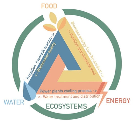
Figure 1.
The interlinkages of the water, food and energy sectors [5].
Traditionally, the different systems in the agricultural sector operate individually and result in different challenges such as resource scarcity, conflicts in the uses of upstream and downstream hydro systems, and also power supply crises due to serious water pollution [6]. The two-way nexus approach has been reported to be used in water distribution network and optimizing wastewater treatment process as a water–energy nexus [7]. Additionally, the energy–food nexus was reported to have been applied in food processing optimization and a water–food nexus was used for irrigation optimization as a two-way nexus [8,9]. However, the utilization of only two-nexus may disregard some important factors or conflicts compared to a more holistic three-nexus approach. Besides that, there is no study that has been carried out on the application of a three-nexus system locally, especially on the agricultural sector. The WFE nexus is therefore a suitable and strategic method to reduce the trade-offs between the separated sectors by creating a system and allowing sustainable development with the interconnectedness of the sectors [2].
The advent of industrialization has caused resource depletion and brought negative impacts on biodiversity. The WFE nexus is able to address the adverse effects by introducing sustainability with the interactions between the sectors. As agricultural production is influenced by the availability of water and energy sources, the complexity of the interrelations between the water, food and energy resources requires a systematic approach to portray the data involved. There is yet to be a clear framework that is able to represent the interconnectedness of the units involved in the WFE nexus. Current nexus approaches applied locally mostly focuses on two-nexus and there is yet to be a three-nexus study in Malaysia’s agricultural sector. While each of the subsystems currently operates separately, the framework designed could deliver the potential interactions between the units included in the three-WFE-nexus.
Furthermore, a suitable approach has to be used to predict the WFE nexus effect in the agricultural sector such as developing a model, conducting experiments or surveying the stakeholders involved. Therefore, an effective model that can track the sinks and sources between the units is urgently needed to manage the wide range of data involved and compute the optimal resource usage that could fulfill the local agricultural demand. Furthermore, the model solution obtained through the system formulated has to be adapted to the local agricultural sector, taking into consideration the potential technologies to be introduced to the local sector.
Another challenge is the necessity to understand the conflicting goals among WFE elements for resource allocation in policy making. With the depletion of resources that is coupled with the growing population, a systematic strategy is needed for the allocation of the limited resources. The model solution obtained has to be interpreted and assessed to increase the efficiency of resource distribution and accuracy of profit prediction when sustainability practice is introduced. The following are the key gaps considered in this paper.
Although there is existing local research in Malaysia involving a two-way water–energy nexus done on water resources management, there is a critical difference between a two-way nexus and three-way nexus, as the latter is a multi-centric concept that addresses the different sectors of water, energy, and food holistically. The WFE-nexus is significant in optimizing resource allocation, but, to the best of authors’ knowledge, a three-way nexus model for the local agricultural sector in Malaysia has not been formulated in any of the reviewed papers.
Despite different conditions and constraints, the reviewed papers involving the three-way-WFE-nexus have mostly focused on the food production system, crops biomass value chain and agricultural waste management. For example, Yuling et al. [10] investigated the centralized local production system considering the nexus integration opportunities for an eco-town in the UK, whilst Garcia et al. [11] assessed the agriculture waste for New York state’s bioenergy production system. Li et al. [12] investigated sustainable bioenergy production incorporating the energy–food–water–land nexus in the Northeast China agricultural system. Nie et al. also put forward an optimization modelling framework to evaluate the allocation and management of agriculture land in China. However, there is yet to have a model in literature revolving only on optimizing the agricultural sector’s resources distribution [13]. Since the resource types and products may vary according to the regions (due to weather conditions, etc.), the three-way nexus models that have been reported in the literature may not meet the conditions to be applied locally in Malaysia too.
Therefore, the main contribution of this paper is the development of the first systematic and integrated model for optimal planning of resource allocation in Malaysia’s agricultural sector. Currently, there is only rudimentary understanding of the complex connections between the resources’ security in Malaysia. There is also insufficient recognition of the security dimensions of these resources, and the problem has to be addressed. The novelty and contribution of this research could be concluded as: (1) multi-objective planning incorporating economic and environmental factors such as economic benefits and carbon emission limit, (2) focusing on the agricultural sector considering geologically-specific crops, livestock, and residents, (3) considering the potential waste recycle systems including wastewater treatment and biomass treatment.
2. Materials and Methods
In this section, the superstructure of a state level agricultural sector is developed based on the Perak state in Malaysia, followed by the model formulation for a preliminary design analysis. The local area studied is well connected to the power grid and therefore energy storage was not considered, and the source of electricity energy in the study is from the power grid. The waste produced by the residential area in the model considers only the gaseous and liquid emissions, where the solid waste such as plastics that may influence the soil and water quality of the agricultural sector is not considered. Besides that, the labour cost involved in the agricultural activities is also excluded, as the main focus is to address the resources allocation such as the residential’s water and electricity usage. The time range of one year is chosen as a basis for the model. Malaysia is a country with almost no seasonal changes in climate, and therefore is not affected by seasons. The starting month for the model designed is taken to be from January.
2.1. Superstructure Construction
As the first step of the nexus design procedure, a geographical area is first selected before constructing the superstructure. A superstructure is then constructed based on the specific sector to show the connection between different subsystems of the units [13]. To construct the superstructure, the sub-units existing in the geographic scope must be defined and classified accordingly. The interconnectedness of the sub-units can be seen clearly in the superstructure, as shown in Figure 2.
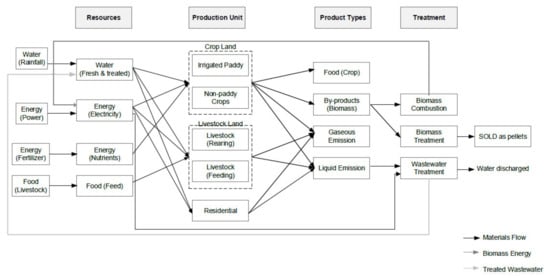
Figure 2.
Superstructure of WFE nexus in the agricultural sector.
As shown in the superstructure, there are three main types of resources; water, energy and food. The water resources are then divided into freshwater and treated water, while the energy resources are divided into electricity energy for water pumping and treatment, and nutrient energy as fertilizer and livestock feed. They are then used by the production units (crops, livestock and residents) to produce different types of products (food, by-products, gaseous and liquid emission). The gaseous emission from the crops considers the direct and indirect carbon emissions, including burning of fossil fuels and biogeochemical processes [14,15].
Finally, the integrated relationship is determined to encourage sustainability by treating contaminated water and unused by-products. The liquid emission from crops and livestock can be reused in the production system as a treated water source through wastewater treatment plants. The crops biomass from agriculture output can be returned into the system by going through biomass treatment as bioenergy. The manure from livestock rearing should also be handled well to prevent air, gas and soil pollution. Manure utilization and treatment technologies should be carefully selected to allow the composts to be reused as organic crops fertilizer.
2.2. Development of Three-Way Nexus Modeling Framework
2.2.1. Mathematical Formulation for Single-Objective Optimization
The modeling of the WFE nexus for the local agricultural sector includes three main steps: constructing a superstructure design for the sector, modeling the units involved in the section, and performing optimization using modeling tools [13]. Due to the complexity of the WFE nexus that includes different sub-units of the agricultural sector, a systematic tool is required to simulate and study the nexus between the key products and treatments, and then further perform model optimization [16]. Nomenclature and data used in this section are elaborated in detail under Appendixe A and Appendix B.
Objective Function
The objective function of the optimization is to maximize the profit of the local agriculture sector, where the production revenue, cost of water demand, cost of electrical energy used for water pumping and wastewater treatment, cost of livestock feed and fertilizer, biomass treatment cost and revenue, and environmental cost of carbon emission are considered:
where = production of crops for product k, = price of crop product k, = water flowrate for unit production j, = cost for 1 m3 of water, = carbon factor for product k, = cost of 1 ton of carbon emission, = biomass used for treatment type l, = cost of biomass by-product treatment l, = price of treated biomass of treatment l, = electricity consumption for unit production j, = energy tariff, = nutrients energy demand from source i, = cost of energy resource i. In general, the cost considered, carbon factor, and biomass factor included in the model equation are fixed values obtained from published literature and government reports.
Constraint on Water Material Balance
The water flow rate that is used in the agricultural sector including crops, livestock and residential usage has to be equally distributed. The total amount of water flowrate used should balance its water demand:
where = water demand from source i and = water flowrate for production unit j.
Constraint on Water Availability
The total water flow rate that is used by the different sectors in agricultural per year, including the crops water consumption, livestock water consumption and residential water consumption must not exceed the maximum available water limit:
where = water flowrate for production unit j and = maximum water flowrate limit.
Constraint on Minimum Water Flowrate
The water usage by the different production units under the agricultural sector must be equal to or exceed its minimum water limit. The water flowrate for the irrigated paddy, non-paddy crops and water used for livestock rearing and cleaning needs to meet its minimum requirement to ensure its products demand. The minimum water flowrate constraint is represented by:
where = water flowrate for unit production j and = water demand for production unit j.
Constraint on the Area Used for Agriculture Production Units
The total area used by the different production units under the agricultural sector, i.e., irrigated paddy, non-irrigated paddy crops and livestock must be equal to or greater than the current land used, which can be represented by:
where = land area for production unit j, = minimum water demand for production unit j, = water flowrate for production unit j, and = total land area used for agriculture production units. The land area for optimal water supply is calculated using the initial land area, divided by the minimum water demand , then multiplied by the variable of the optimal water supply .
Constraint on the Land Limit for Agriculture Production Units
The land area that is available for the agriculture sector production units is limited. Therefore, the area used by the different production units under the agricultural sector including irrigated paddy, non-irrigated paddy crops, and livestock should be equal to or less than the land limit:
where = land area for production unit j, = minimum water demand for production unit j, = water flowrate for production unit j, and = maximum land available for agriculture production. The land area for optimal water supply is calculated using the initial land area, divided by the minimum water demand , then multiplied by the variable of the optimal water supply .
Constraint on Wastewater COD levels
The wastewater from various sources of the agricultural production units has to be treated before flowing into sinks for reuse, as the water sinks can only accept water with a standard level of chemical oxygen demand (COD). The COD level concentration balance for wastewater is as below:
where = COD removal efficiency of wastewater treatment plant, = COD level of the wastewater from sources of production unit j, = wastewater amount from sources of production unit j, = COD level of treated water of production unit j flowing to sinks, and = treated water amount of production unit j flowing to sinks.
Constraint on Minimum Energy Required for Water Pumping and Treatment
The energy required to supply water for the different production units such as irrigated paddy, non-irrigated paddy crops, and livestock must be equal to or greater than the current total electricity used for the agriculture sector:
Where = total water pumping and treatment energy used for agriculture production units, = water pumping energy for production unit j, = minimum water demand for production unit j, = water flow rate for production unit j, = treated wastewater for production unit j, and = energy required for wastewater treatment for production unit j. The energy required for pumping and treatment was calculated based on the amount of water that is involved in the process. The energy required for optimal water pumping is calculated by dividing the minimum energy required, by the minimum amount of water demand, and then multiplied by the variable of water required by the production unit, .
Constraint on Primary Electricity Supply
The total electricity that is used by the agricultural sector must not exceed the primary electricity supply that is available:
where = electricity consumption for unit production j and = primary electricity supply.
Constraint on Minimum Electricity Demand
The electricity that is used by the different production units under the agricultural sector has to be equal to or exceed its minimum electricity energy required. The minimum electricity demand constraint is to ensure the outcome of the production units:
where = electricity consumption for unit production j and = minimum electricity demand for production unit j.
Constraint on Minimum Nutrients Required
The total energy in nutrients form that is required by the production units including irrigated paddy, non-irrigated paddy crops, and livestock has to be equal to or greater than the minimum nutrients that are required by the agricultural sector:
where = water pumping energy for production unit j, = minimum water demand for production unit j, = water flowrate for production unit j, and = total energy in nutrients form required by agriculture production units.
Constraint on Minimum Residential Energy Demand
The total energy that is provided by the production units, including the irrigated paddy, non-irrigated crops, and livestock has to be equal to or more than the minimum energy demand that is needed by the residents:
where = water pumping energy for production unit j, = minimum water demand for production unit j, = water flowrate for production unit j, and = residents food energy requirements.
Constraint on minimum crop amount
The crop production of the irrigated paddy, palm oil, and rubber has to be equal to or greater than the minimum crop amount needed. Each production unit has its minimum requirement for the product amount to meet to ensure its consumers’ needs. The minimum crop amount constraint is represented as below:
where = production of crops for product k and = minimum crops demand of product k.
Constraint on Area Distribution for Crops
The total area used for the crop production has to be equal to or greater than the total current area used for the different types of crops:
where = land area for crop production j, = minimum crops demand of product k, = crop production for product k, and = total land area used for crop production.
Constraint on Carbon Emission Limit
The carbon emitted by crop production, livestock and residents should be equal to or less than the carbon emission limit. The carbon factor was obtained through literature, where the direct and indirect carbon emissions of the crops are considered. The CO2 emission level should meet the requirement for the reduction to ensure it is controlled:
where = amount of products from production unit j, = carbon factor for crop product j, and = carbon emission limit.
Constraint on Biomass By-Product
The biomass factor determines the amount of palm oil biomass that can be produced by a hectare of palm oil plantation that can be sold for further biomass treatment. The amount of palm oil by-products is calculated as below, where the biomass factor was obtained from the Malaysian Palm Oil Board (MPOB):
where = area used for palm oil plantation, = biomass factor for palm oil crops and = biomass by-product produced.
Constraint on Biomass Combustion and Treatment
The biomass by-products produced by the palm oil mill and plantations can be further processed to be recycled back to the sector. The biomass can be combusted and turned into a power supply through steam or be processed into pellets to be sold as profit:
where = biomass by-product produced, = biomass used for treatment type l.
2.2.2. Multi-Objective Simultaneous Design
There are two optimizations performed and the results obtained are being compared. The single-objective optimization is first performed by taking into consideration the subsystems interactions simultaneously. The variables defined includes the water demand, the crops production and the electricity demand for residential, irrigated paddy, non-paddy crops and livestock, respectively. The objective of the optimization is to maximize the profit of the local agricultural sector.
Following that, the multi-objective linear programming optimization is also performed. The first objective function considers minimizing the water consumption for the agricultural sector, including the water usage for irrigated paddy, non-paddy crops and livestock. The multi-objective optimization is performed for validation and calibration of the results by comparing with the base case of the single-objective optimization. This is because real life data are not available since this is the first three-way WFE nexus model developed for the Malaysia agricultural system:
where = water flowrate for unit production j. The second objective function maximizes the revenue of the total crops production including the crops produced by the irrigated paddy, palm oil and rubber.
where = production of crops for product k and = price of crop product k. The third objective is to maximize profit as investigated in the single-objective optimization, where the profit is calculated as:
where = production of crops for product k, = price of crop product k, = water flowrate for unit production j, = cost for 1m3 of water, = carbon factor for product k, = cost of 1 ton of carbon emission, = biomass used for treatment type l, = cost of biomass by-product treatment l, = price of treated biomass of treatment l, = electricity consumption for unit production j, = energy tariff, = nutrients energy demand from source i, = cost of energy resource i.
MINIMAX Goal Programming
The multi-objective optimization is performed by applying the MINIMAX goal programming method algorithm as follows:
where D = maximum deviation, = negative deviation from the target value and = negative deviation from the target value, and = respective positive weights of the negative and positive deviations:
where is a linear objective function of x, = negative deviation from the target value and = positive deviation from the target value and = target value of the objective.
Objective Weights
For the multi-objective optimization, the weights for the different objectives are needed to be able to solve the linear programming model. The preference weights to be used for each of the objectives are selected using the Analytic Hierarchy Process (AHP) [17]. The weights that are used in solving the mathematical model are denoted as w1, w2, and w3 for the objectives minimizing water usage, maximizing crops yield and maximizing total profit, respectively. There are four different scenarios that are considered, where Scenario 1 assumed that the importance of the three objectives is equal, and the weights are set at 0.3333 for w1, w2, and w3.
For the other scenarios based on AHP, it is assumed that one of the three objectives is the most significant, while the other objective is subordinate to it, and the objective left is the least significant. The weights for the objectives in this situation would be 0.6370, 0.2583 and 0.1047, respectively, for solving the model. For example, in Scenario 2, the objective that is set to be the most significant is minimizing the water usage, followed by maximizing crops yield, with maximizing the total profit as the least significant objective. This will result in the objective weights of w1 = 0.6370, w2 = 0.2583 and w3 = 0.1047. The significance of the objectives in Scenario 3 is maximizing crop yield, followed by minimizing water usage and maximizing total profit, while in Scenario 4 the order of objectives significance is maximizing total profit, minimizing water use and maximizing crops yield. A semantic 9-point scale consisting of priority values of 1, 3, 7 and 9 corresponding to the levels of importance pair-wise comparison matric is applied.
2.3. Sensitivity Analysis
After obtaining the optimal solution, sensitivity analysis was performed to study and evaluate the uncertainties of the variables and constraints involved in the model. The parameters involved in the model are varied between the planned ranges, respectively. The sensitivity of the optimal solution on the constraints and the effect of the parameters on the coefficients in the objective function are analyzed and evaluated through the sensitivity report obtained.
2.4. Case Study on Perak Agricultural Sector
The agricultural sector of Perak state in Malaysia is selected as a case study for the WFE nexus approach as the economy of the state is mainly driven by agriculture. The population of the Perak state is 2.51 million by 2021 and the land distribution in Perak is mainly forest reserve, agriculture and industry buildings [18]. The main resources available in Perak are water and energy. Water resources in the sector are mainly freshwater supplying the agricultural, industrial sector and domestic use. The main freshwater source in Perak is from rivers, where 45% of freshwater is from Sungai Perak, followed by Sungai Kinta and Sungai Sungkai [19]. Besides that, energy used in the Perak agricultural sector is electricity energy and nutrients energy. As the geography of the Perak state is not a flat surface land, energy will be needed to pump water from the source to be distributed to the land that needs water for irrigation and livestock. Other than that, livestock will also need food intake while crops require fertilizer, which is also an energy source.
The main industrial crops in Perak are the irrigated paddy, palm oil and rubber plantations. From these three main crops, the oil palm crops have the highest production (207,900 kg/year) followed by paddy (3425 kg/year) and rubber (1221 kg/year) [20]. The main livestock in Perak are cattle, goat, swine, poultry and duck, which is tabulated as shown in Table 1.

Table 1.
Livestock population in Perak by 2020 [21].
The case study also takes into consideration the land available in Perak that can be used for the agricultural sector. As the land that is ready to be used by the sector is limited, the land for the crops and livestock production has to be optimally distributed. The mathematical formulation modelled in this section is based on the Perak agricultural sector case study, where a specific crop types, livestock, and waste management is assumed based on the case study area to show a clearer concept of the nexus system. With minor adaptions, the model developed can be improvised to be applied in an arbitrary sector.
3. Results and Discussion
The agricultural sector of Perak state in Malaysia is selected as a case study for the WFE nexus approach as the economy of the state is mainly driven by agriculture. A single-objective optimization is performed with its objective function to maximize profit, followed by a multi-objective optimization using a MINIMAX approach. The results obtained are then evaluated through sensitivity analysis.
3.1. Superstructure of Perak Agricultural Sector
The superstructure of the agricultural sector in Perak is then constructed, where the industrial crops and the livestock are selected to be the production system in the model. Other subsystems in the sector are the resources, land types, product types, and treatment. The sinks and sources of the units can be shown in the superstructure and the interconnectedness can be studied as shown in Figure 3.
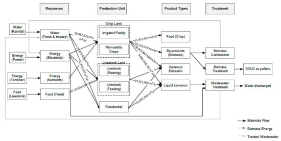
Figure 3.
Superstructure of the Perak local agricultural system.
The flow of the water, energy, and food resources in the sector can be seen in the superstructure, as well as the interconnections between the resources. Through the nexus system, other alternative pathways for resources recycling in the agricultural sector are introduced, where biomass by-products from the crops are treated to supply biomass energy as a potential energy supply. Besides that, wastewater generated from the food and energy production is also treated to be reused in the water supply system. The mathematical formulation is then developed based on the connections studied through the superstructure, where the size of the model is determined by the units considered, and is flexible with the production units, product types and treatment technologies introduced. In this case study, the energy sources considered includes fertilizer and power supply, without power generated from power plants as the focus is on the resources distribution in the agricultural sector.
Input Data
The objective of the single objective optimization is to maximize the local agricultural sector profit which takes into consideration the freshwater cost, energy cost, fertilizer and food cost, revenue from the crops production, carbon emission cost, and revenue from the palm oil biomass. Table 2 shows the data values that are used in the model to calculate the optimal solution, where information from previous published literature and government reports are used to calculate and estimate the resources consumption. The variables set in this mathematical model are the freshwater flowrate for the irrigated paddy, non-irrigated crops, and livestock, as well as the crop amount of the plantations in Perak. The model is then solved using simplex linear programming with the objective and constraints.
Table 2.
Data values for Perak state used in the mathematical model.
The water in this model is required for residential use, crops irrigation and livestock cleaning and rearing. Besides that, the crops produced are sold and considered in the final profit of the agricultural sector. Electricity is required by the water pumping and distribution, as well as the wastewater treatment. The CO2 emission is expected to reduce by 50% compared to the CO2 emission by the crops in 2005 [35]. The CO2 that exceeded the GHG emission limit will be charged an environment penalty of Ringgit Malaysia (RM) 4.03/tCOe carbon tax [36]. The details data information used in the model are explained in Appendix B.
3.2. Optimization Results
3.2.1. Single-Objective Optimal Solution
The optimal profit obtained in the Perak agricultural sector is estimated at RM 5.50 billion. In comparison with the state’s agricultural sector profit in 2015 of RM 8.6 billion, the total profit reduced by RM 3.1 billion [18]. The possible reason of the reduced profit is the introduction of waste management and conservation technologies including biomass treatment to the palm oil byproducts and local sustainable wastewater treatment. The carbon pricing for CO2 emission from the crops production is also introduced in the model to control carbon emission and reduce pollution for environment conservation and long-term planning of the agricultural sector. The freshwater flowrate, electricity consumption and the amount of crop production are the variables that are optimized. Table 3 shows the initial and optimized values of the variables as comparison, where the initial values are the initial data values used at the start of the optimization, and the optimized value is obtained from the optimal solution of the optimization.
Table 3.
Variables in the model that are optimized with their initial values.
By comparing the initial and optimal values, it can be seen that the freshwater and electricity demand of the irrigated paddy increases significantly, as well as the paddy crop production that increases by more than twice the initial production. It is assumed that the distribution of the water and energy resources to the paddy crops is due to its lower wastewater COD value and carbon emission factor compared to the non-paddy crops and livestock. The wastewater COD value of the irrigated paddy, non-paddy crops and livestock are 160 mg/L, 41,125 mg/L and 2210 mg/L, respectively, while the carbon emission factor for the irrigated paddy, palm oil, and rubber crops are 1.06 kgCOe/kg, 3.18 kgCOe/kg, and 2.93 kgCOe/kg, respectively [14,30,31,32]. This shows that the environmental factor is taken into consideration while distributing the resources as wastewater treatment cost and carbon emission cost are included in calculating the sector’s profit. It can also be seen that there is an increment of the crops production for the irrigated paddy, palm oil, and rubber. This means that, by practicing the nexus system and introducing waste treatment technologies, the resources that are distributed into the agricultural sector will be utilized efficiently in the food production system.
It can also be observed that, for an increase in paddy crop amount of 2.3, there is an increase of 13 times the amount of water and electricity required. The reason for such high value is probably due to the minimum electricity demand that is currently used by the agricultural sector that are not negligible. This is to meet the current total electricity required for water pumping and allocation, including the surplus rainfall. As there is no upper limit or constraint on the water supply, the surplus water is also being distributed unnecessarily to the crops area. This shows that the water crisis currently being experienced by the Malaysia’s paddy crops is not about too little water but a proper water management, where the crops are receiving more than the required water demand [37]. Hence, a proper management of the water supply to increase the productivity and water-use efficiency of the paddy crops production is needed. As an example, if the surplus rainfall and current electricity used for water allocation is not considered, the water demand for the irrigated paddy will decrease to 2,292,768,478 m3/year. This shows an increase of only 1.7 times of water to increase the production of paddy crops by 2.3 times. This scenario can be achieved provided that the water management is able to address appropriately the surplus water available and, consequently, the electricity used for water allocation can be decreased.
The distribution of the production units (irrigated paddy, non-paddy crops, livestock) and the production of the crops (irrigated paddy, palm oil, rubber) are shown in Figure 4 and Figure 5. The initial distribution and the distribution after optimization for different constraints are shown in bar charts with their percentage values.
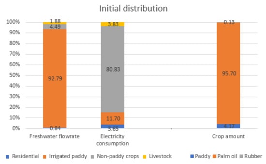
Figure 4.
Initial percentage distribution production units and crops production.
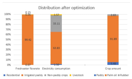
Figure 5.
Percentage distribution after optimization.
For the freshwater flowrate for production units’ consumption, the irrigated paddy has the highest water consumption (92.79%) followed by non-paddy crops (4.49%), then livestock (1.88%) and residential area (0.84%). The irrigated-paddy water flowrate percentage increases to 99.42% as there is a higher water consumption. Other than that, the electricity consumption for water distribution and treatment was mostly consumed by non-paddy crops that takes up to 80.83%. After optimization, the electricity consumption is more equally distributed where non-paddy crops consume 33.11% electricity and irrigated paddy consumes 63.83% electricity. For the crops production in ton/year, the palm oil crops contributed to most of the production in Perak’s agricultural sector. The initial percentage of the palm oil crops was 95.7% and, after optimization, it is 91.89%. The contribution of the irrigated paddy crops increased from 4.17% to 5.48%, while the rubber crops contribution also has an increase from 0.13% to 2.63%.
It can be observed that there is a significant increase in the electricity consumption percentage for irrigated paddy. The increment of the electricity consumption is due to the high-water requirement of the paddy crops, causing it to be more dependent on electricity for pumping, delivery and treating the water used for the crops. This result aligns with the research done by Leung [10], where electricity consumption is higher when potato production is involved as the crop is more dependent on this input. When a crop that has a higher dependent on the electricity is involved, it will affect the result of the food subsystem design.
The revenue contributed to the profit and the cost distribution for the profit in the local agricultural sector in Perak are shown in Figure 6. The crops production contributed to most of the revenue while the treated biomass contributes to 23.74% of the revenue. From the crops production, palm oil contributed to 68.38% of the sector’s revenue, followed by rubber, 4.35% and paddy crops, 3.52%. As the biomass revenue is also contributed by the palm oil crops, it can be concluded that palm oil brings a larger positive economic impact to the Perak’s agricultural sector. This agrees with the statistics provided by Department of Statistics Malaysia (DOSM), stating that palm oil is the major contributor to the agriculture sector’s gross domestic product (GDP) at 46.6% [38]. However, the high carbon emission from the palm oil crops also has the highest negative environmental impact and should be considered while focusing on the development of the crops.
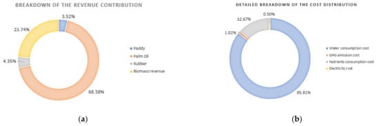
Figure 6.
Detailed breakdown of the (a) revenue distribution and (b) cost distribution for the total profit objective function.
Besides that, for the cost distribution, the local water consumption requires the most amount of cost, contributed to 85.81% of the costs. It is followed by the nutrients’ energy cost, greenhouse gas (GHG) emission cost and electricity cost. It can then be concluded that the agricultural sector is highly dependent on the water resources, and the government could consider providing subsidies for crops and livestock water consumption to encourage the development of the agricultural sector.
3.2.2. Multi-Objective Optimal Solution
To further study the coefficients in the single objective, multi-objective optimization is performed. The objective functions minimizing water usage is optimized for resource conservation, while simultaneously ensuring crops production and the resulting economic impact.
The boundaries of the objectives are obtained by determining the minimum and maximum value through solving it as a single objective function for each of the objectives. From Table 4, the boundaries of the water usage are 1.811 × 10¹⁰ m3/year and 2.213 × 10¹⁰ m3/year, while, for the crops yield, the boundaries are 1.661 × 10¹⁰ RM/year and 2.992 × 10¹⁰ RM/year which are the minimum and maximum values of the objective functions, respectively. For the profit objective function, the upper and lower boundaries are −15.81 × 10⁹ RM/year and 7.078 × 10⁹ RM/year. The negative minimum value of the profit objective function shows that prioritizing other demands will result in a higher cost then revenue, causing a loss in the economic aspect. The results obtained through multi-objective optimization will be a trade-off of the three conflicting objectives within the respective boundaries.
Table 4.
Optimization solution at different scenarios.
The optimization solution of the objectives is also affected by the weightage that determines the significance of the different objectives in a multi-objective optimization. For example, the water usage amount in Scenario 1 gives a value that is at the middle range between the water usage amount among other scenarios. The water usage amount is the lowest in Scenario 2 where the objective of water usage is given priority with the highest weightage, and the water usage is higher in Scenarios 3 and 4 when the priority is focused on the other two objectives, maximizing crops yield and profit. This shows that the water usage will be affected and increased when other objectives are considered and focused on. The increase of water usage when the objective functions of maximizing crops yields and profit is considered agrees with the results obtained by Li et al. [12], where the bioenergy production decreases when the cost and environmental impact are included in the model.
On the other hand, objectives involving crops yield and economic impacts have the highest value when the weights are prioritized, as the main purpose of both objectives is to be maximized. This can be seen when the objective of maximizing crops yield obtains a value of 2.98 × 10¹⁰ RM/year in Scenario 3 when it has a higher weightage, and, in Scenario 4, the objective of maximizing total profit has a value of 5.761 × 10⁹ RM/year. Both values obtained by the two objectives in the respective scenarios have higher values resulting from the given prioritized weight compared to the other scenarios. This agrees with the findings of Yue et al. [39], where the multi-objective model will compromise among contradicting objectives, providing the optimal value in its own focus without other key considerations.
The multiple solutions obtained by altering the weights could provide more alternatives for decision makers as a guideline while planning the resource allocation including water, nutrients energy, electricity, and land.
3.2.3. Distribution of Resources to the Agricultural Sector’s Sub-System
The resources that are involved in the agricultural sector’s WFE model include the water supply, electricity energy, nutrients energy such as fertilizers and food supply. The resources are then distributed to three main production units in the sector, which are the crops plantation, livestock rearing and residential involved in the agricultural sector. This section discusses the distribution of resources based on the optimal solution of the single-objective model. The water usage for the single-objective model is 1.85 × 10¹⁰ m3/year, which is distributed to the residential, crops and livestock, respectively, as shown in Figure 7.
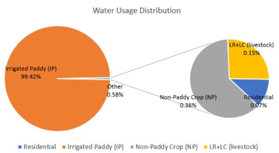
Figure 7.
Distribution of water usage in the agricultural sector.
It can be seen from Figure 7 that most of the water usage is distributed to irrigated paddy crops (99.39%), followed by non-paddy crops (0.35%), livestock (0.19%) and residential area (0.07%). Non-paddy crops require 6.54 × 10⁷ m3/year water supply which includes rubber and palm oil, while the livestock including cattle, goat, swine, poultry and duck requires 3.56 × 10⁷ m3/year water supply for rearing and cleaning which takes up 0.35% and 0.19% water usage, respectively. The residents that are involved in the agricultural sector as manpower will also require 1.23 × 10⁷ m3/year water supply that contributes 0.07% of water usage. The irrigated paddy has a higher percentage with its water supply of 1.84 × 10¹⁰ m3/year as it will require a higher amount of water supply and has a higher minimum water demand compared to other crops in the sector [22].
The model solution of the variables that is involved in the local agricultural sector crop production can be seen in Figure 8. It can be seen that the palm oil production has a yield of 3.48 × 10⁷ ton/year, which contributes to 95.66% of the crops production, followed by rubber production with its yield 8.88 × 10⁵ ton/year contributing to 2.44% of crop production. The paddy crop has a lower yield of 6.92 × 10⁵ ton/year occupying 1.90% of crop production. It can be seen that the paddy crops have the lowest contribution to the total crops production, despite the fact that it has a higher resources consumption of the water and energy as seen in Figure 7 and Figure 9. Although paddy crops have relatively low crops production, most of the resources are distributed to the paddy due to its qualities, including low fertilizer consumption, low wastewater COD level and low carbon emission. By considering the WFE nexus, the paddy crops have a higher positive environmental and economic impact, compared to other crops when the fertilizer cost, wastewater treatment cost, and carbon emission cost are considered.
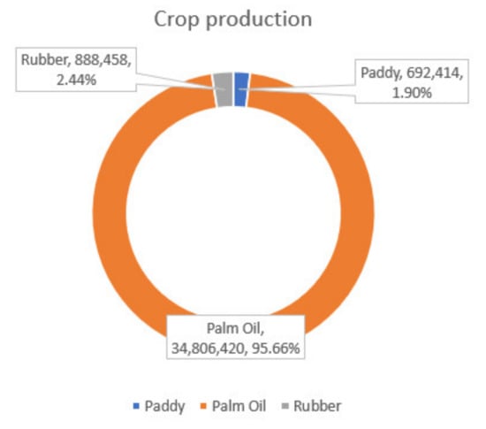
Figure 8.
Contribution of crop production in the agricultural sector.
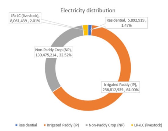
Figure 9.
Electricity supply distribution in the agricultural sector.
The distribution of the electricity energy in the agricultural sector can also be seen in Figure 9. The irrigated paddy requires the most electricity supply of 2.57 × 10⁸ kWh/year distributing to 64% of total electricity consumption, followed by non-paddy crops such as rubber and palm oil that requires 1.3 × 10⁸ kWh/year that takes up 32.52%. The livestock requires 8.06 × 10⁶ kWh/year electricity that takes up 2.01% of electricity supply while the residents household involved in the agricultural sector contributes to 1.47% of electricity consumption of 5.89 × 10⁶ kWh/year. The electricity consumption in the agricultural sector is required for water pumping and distribution, as well as wastewater treatment for recycling treated water that conserves water resources. Water and electricity distribution are mutually connected in the agricultural sector, and the high electricity consumption of the paddy crops is due to its highly water-intensive feature, causing it to be highly dependent on electricity for water pumping and treatment [40]. The breakdown of the electricity distribution is shown in Figure 10.
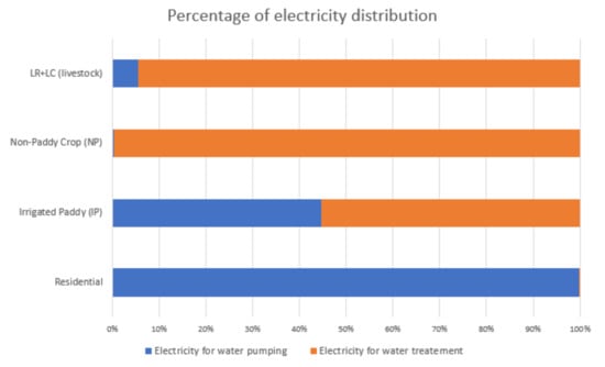
Figure 10.
Percentage of electricity distribution in the agricultural sector.
It can be seen in Figure 10 that more than half of the electricity supplied to the crops and livestock is used for wastewater treatment, while for the non-paddy crops, more than 99% of electricity is used for wastewater treatment. This is due to the high COD level in the wastewater produced by the rubber and palm oil crops, which are 50,000 mg/L and 32,2350 mg/L, respectively [31,32]. The high COD level in the wastewater will require more electricity for wastewater treatment to meet the standard COD level at 100 mg/L under Class III, which is safe to be used for agricultural activities including irrigation and livestock use [41]. The livestock effluent also has a high COD level of 2210 mg/L compared to irrigated paddy, which is 160 mg/L, resulting in a higher electricity requirement for wastewater treatment [29,33].
3.3. Result Analyses
To further study and understand the relation between the model coefficients and the optimal solution, sensitivity analysis was performed. The sensitivity of the optimal solution on the constraints and the objective function can be further investigated.
3.3.1. Single-Objective Optimization Variables
Variables
There are eleven variable cells in the model, including the water and electricity demand of the residential area, irrigated paddy, non-paddy and livestock, and the crop production of paddy, palm oil and rubber. The value of the optimal solution will affect the final objective function, where the optimal value of this model is 5.47B RM/year.
From the sensitivity analysis of the variable cells as shown in Table 5, the reduced cost of the non-paddy water demand is −2.42 RM/year. The reduced cost of the non-paddy water demand shows that, if the variable is increased by a unit (m3/year), the total profit will be decreased by −2.42 RM/year. Therefore, it is not advised for the non-paddy water demand to be increased, as it will reduce the final profit. Compared to the residential and crops water demand of −1.03 RM/year and −2.42 RM/year, the livestock water demand has a higher value of −145.56 RM/year. Hence, it can be concluded from the sensitivity analysis of the variable cell that the livestock rearing is much more dependent on water compared to crops production.
Table 5.
Variable cells’ sensitivity analysis.
Besides that, the reduced cost of the electricity demand of the residential, crops, and livestock are −0.428 RM/year. The negative values of the reduced costs show that a unit increase in production will negatively affect the final profit. Therefore, the electricity demand variables should not be increased as the objective function is to maximize the local profit. The reduced cost is nonzero only when the variable’s value is equal to its upper or lower bound at the optimal solution. By studying the variables with nonzero reduced cost, it can be observed that the initial and optimal values remained unchanged, showing that the variable is in its upper or lower limit. This validates the nonzero reduced cost of the variables.
Constraints
For the sensitivity analysis on the constraints, there are a few constraints that are studied in this model as shown in Table 6. The constraints can be categorized into binding and non-binding constraints, where a binding constraint is a non-zero value and is equal to its bound that can affect the final result, while a non-binding constraint does not affect the final optimal solution.
Table 6.
Constraint’s sensitivity analysis.
The shadow price of the energy required for water pumping constraint is −259 RM/year. This shows that increasing the constraint by one unit (kWh/year) will result in a decrease in the total profit by 259 RM/year. In addition, note that, when the shadow price of a constraint is nonzero, the final value and the right-hand side (RHS) value are the same. This indicates that all of the available units of the constraints have been used. The shadow price of the land available for the crops production constraints are 7.23 × 10³ RM/year. 6.84 × 10⁴ RM/year and 6.65 × 10³ RM/year for irrigated paddy, palm oil and rubber, respectively. This demonstrates that the land available for the crops is totally used.
On the other hand, a shadow price of zero indicates that an additional unit increase of the constraint’s value will not increase the objective function value or the sector’s profit. As an example, for the freshwater availability constraints, the final value of the freshwater supply is 1.81 × 10¹⁰, whereas the RHS value of the constraints is 2 × 10¹⁰. This indicates that we have not used all of the freshwater available, and this explains the zero shadow price value of the constraint. The resources with zero shadow price including water and electricity, as well as the carbon emission limit, are still available for further uses. This confirms that the optimal solution obtained takes into consideration the environmental factors.
The reduced cost for the variables cell and the shadow price of the constraints cell could act as a guideline so that accurate and data-driven decisions or policies can be implemented for resource allocation.
3.3.2. Multi-Objective Optimization
The obtained result of the optimization model is analysed to study the relationship between the three objectives. The interaction between the water consumption and the crops yields objective functions are studied by assuming a constant deviation weight for the total profit objective, 0.5. The weights of the water usage and crops yields objective function are altered between 0.05 to 0.45 with a difference of 0.05, where the sum of the weights add up to 0.5. The values of the objectives are then calculated where the model solution is shown in Figure 11.
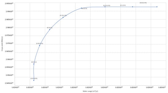
Figure 11.
Relationship between the water usage and crops yield objective functions.
From Figure 11, when the weight of the crops yield function increases and the weight of the water usage objective function decreases, the water usage and the crops yield will increase. The values shown on the points in the graph denote the deviation weights used for the objective functions, where the first value represents the weight used for the water usage objective, and the second value corresponds to the crops yield function. It is also worth noting that the last few points have a small difference due to the upper limit of the resources. The same method is also applied in studying the relationship between the objective functions 1 and 3 (the water usage and total profit), and then results are shown in Figure 12.
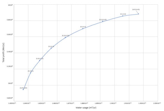
Figure 12.
Relationship between the objective functions of the water usage and profit.
The relationship is investigated by assuming the deviation weight of the crops yield objective function as 0.5, while changing the deviation weights of the studied objective functions ranging from 0.05 to 0.45 with an interval of 0.05. As shown in Figure 12, when the deviation weight of the total profit objective function increases and the weight of the water usage objective function decreases, the total profit of the agricultural sector and the water usage will increase. This shows a contrast between the two objectives, where the aim is to decrease the water usage while increasing the total profit.
The Morris screening method is further used for local sensitivity analysis to study the model results obtained [42]. The effect of changes in the parameters such as the crop planting area and the variable cost on the final water usage and total profit in Scenario 1 is examined. The results are shown in Figure 13 and Figure 14, where the steady trend of the graphs shows that the model solution is accurate with a positive behavior.
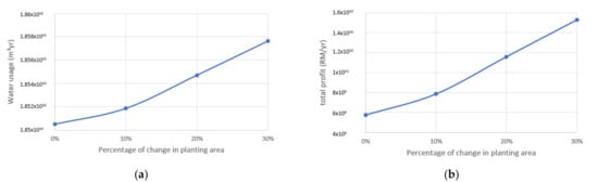
Figure 13.
Percentage deviation of (a) water usage and (b) total profit objectives with percentage changes in crops planting area.
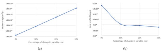
Figure 14.
Percentage deviation of (a) water usage and (b) total profit objectives with percentage changes in variable cost.
As shown in Figure 13, when the crops planting area increases, the water usage of the agricultural sector will increase as well, where the value of the model solution is further from the base case value in Scenario 1. The total profit, on the other hand, increases with the increasing crops’ planting area. This indicates that, when the crops planting area increases, a higher amount of resources including water supply is required, producing more crops and results in a higher total profit. Such results show, with the utilization of the available resources, the agricultural sector’s economy can be supported efficiently.
It can also be seen in Figure 14 that the increasing of the variable costs in the model will result in an increase in the water usage and a decrease in the total profit. This shows that, when the cost of the resources and crops increases, there will be a higher requirement in the water supply to produce enough crops to meet the agricultural economic requirement. The reduction in the total profit of the sector also shows that the investment in the available resources would not be able to sustain the sector economically when the cost of water and crops increases. This result aligns with the results obtained by Mahjoub and Sahebi [43], where there is an increase in the cost requirement when the variable costs increase. It is therefore important to efficiently distribute and conserve the available resources to prevent shortage and fluctuation of the resources cost in the future. The indistinct changes of the results value can be improved by obtaining a robust solution, where the resource based sensitive parameters are altered.
The case study illustrates how the interactions between the different resources can be systematically analyzed after the application of the nexus system. The insights that are not intuitively obvious could be obtained through analyzing the results, and therefore the practice preliminary design analysis is essential.
4. Limitations and Future Work
Firstly, the crop productions are assumed to be “near-optimal” where the crops produced are at a fixed amount in the period of time (yearly) studied. This was done to decrease the computational demands of the model optimization, and it may cause an underestimation of the real potential yield. Future works could consider studying the proposed model in an uncertainty state by including the dynamic cropping patterns, such as including the main and off seasons of the crops. This can be done by utilizing the robust optimization methods.
Other limitations are the electricity energy considered in the model. The model developed in the study considers the electricity energy distributed from the power grid, where the power generation for electric energy, and the machinery oil and gas energy used for transportation were not included. Further studies should consider the generation of power from fossil fuels or renewable energy, as energy in agriculture is an intermediate input and emission.
In terms of labour cost, if the section is considered in the model, the total labour cost for the agricultural sector would be RM0.703 billion per year. This can be calculated with the estimated labour involved in the agricultural sector of 36,637 workers in the Perak state [27], and the labour cost with an average monthly salary per employees in the agriculture of RM1600 [44]. Therefore, with a yearly income of RM19,200 per household, the total labour cost can be calculated to be 0.7B RM/year, and this will further deduct the profit of the agricultural sector to be 4.8B RM/year from 5.5B RM/year.
Besides that, the current work only focuses on developing the WFE nexus system in the local agricultural sector from scratch, and limitations such as data availability and the feasibility of implementing the model has to be considered. This includes studying the adaption of the model for retrofitting existing systems in future works.
5. Conclusions
With the increasing population and food consumption, it is challenging to be able to meet the growing demand with the limited water, energy and land resources. Therefore, it is important to develop a model to be implemented in the local system that could support decision-making to practice sustainability. A WFE nexus optimization model for the local agricultural sector is developed in this study and is further applied in Perak state as a case study.
The superstructure developed based on the case study in Perak shows the relationship of the different subsystems and the interconnectedness of the units can be studied. Besides that, the case study single-objective model solution is able to quantify the values for each component, identifying the trade-offs for the production units and crop production while maximizing local agricultural sector profit. From the results, it can be concluded that irrigated paddy crops could contribute to a higher profit compared to palm oil and rubber crops. Thus, future development can be focused on irrigated paddy crops while meeting other constraints and demands to ensure that the resources are optimally utilized. The multi-objective optimization solved using MINIMAX also provides decision-makers with a guideline that implements the WFE nexus locally in the agricultural sector. Sensitivity analysis performed also proved that the model is computationally efficient, and the trade-offs among WFE elements should be considered while making informed decisions for WFE nexus management. The simultaneous multi-objective optimization sensitivity analysis also demonstrated how these types of analyses can be useful for policy and decision-makers while practicing WFE nexus management.
The work presented in the research only concentrates on developing the model of the local agricultural system. The resources’ demand and costs are calculated as the “near-optimal” values, where it may result in an underestimation of the real potential socioeconomic demands and cost-related parameters. Future modelling work should explore the adaption of the model for retrofitting existing system and dynamic parameters to minimize the gap between simulating values and real potential values. The present work has captured the interconnections between different subsystems and the existing risk of introducing the WFE nexus locally can also be prevented by performing simulation before execution. This study will provide an overview of the WFE system that helps with planning the rules and guidelines before applying them in the community.
Author Contributions
Conceptualization, Q.S. and H.Z.; methodology, Q.S.; software, Q.S.; validation, Q.S.; formal analysis, Q.S. and H.Z.; investigation, Q.S.; resources, Q.S.; data curation, Q.S.; writing—original draft preparation, Q.S., writing—review and editing, Q.S. and H.Z.; visualization, Q.S.; supervision, H.Z.; project administration, H.Z.; funding acquisition, H.Z. All authors have read and agreed to the published version of the manuscript.
Funding
This research was funded by The Murata Science Foundation 2020 Cycle 1, Grant No. 015ME0-184.
Institutional Review Board Statement
Not applicable.
Informed Consent Statement
Not applicable.
Data Availability Statement
Not applicable.
Conflicts of Interest
The authors declare no conflict of interest.
Appendix A
Nomenclature
Sets and Indices
| Resources | |
| Freshwater and treated water resources | |
| Electricity energy source for water pumping | |
| Nutrients’ energy source comprising fertilizer and livestock feed | |
| Production units | |
| Crops and livestock production units | |
| Paddy, palm oil and rubber production units | |
| Product types | |
| Paddy, palm oil and rubber crop products | |
| Waste treatments | |
| Combustion and processed pellets biomass treatments |
Parameters
| Price of crop product k | |
| Cost for 1 m3 of water | |
| Carbon factor for product k | |
| Cost of 1 ton of carbon emission | |
| Cost of biomass by-product treatment l | |
| Price of treated biomass of treatment l | |
| Primary electricity supply | |
| Minimum electricity demand for production unit j | |
| Energy tariff | |
| Nutrients’ energy demand from source i | |
| Cost of energy resource i | |
| Water demand from source i | |
| Maximum water flow rate limit | |
| Water demand for production unit j | |
| Land area for production unit j | |
| Minimum water demand for production unit j | |
| Total land area used for agriculture production units | |
| Maximum land available for agriculture production | |
| COD level of the wastewater from sources of production unit j | |
| Wastewater amount from sources of production unit j | |
| COD level of treated water of production unit j flowing to sinks | |
| Treated water amount of production unit j flowing to sinks | |
| Energy required for wastewater treatment for production unit j | |
| Water pumping energy for production unit j | |
| Total water pumping and treatment energy used for agriculture production units | |
| Total energy in nutrients form required by agriculture production units | |
| Residents’ food energy requirements | |
| Minimum crops demand of product k | |
| land area for production unit k | |
| Total land area used for crop production | |
| Amount of products from production unit j | |
| Carbon factor for crop product j | |
| Carbon emission limit | |
| Area used for palm oil plantation | |
| Biomass factor for palm oil crops | |
| Biomass by-product produced |
Variables
| Production of crops for product | |
| Water flow rate for unit production j | |
| Electricity consumption for unit production j | |
| Biomass used for treatment type l |
Appendix B
Data Used for Model Optimization
The data used for solving the model were obtained from the official government’s data base, government agencies, international organizations and open literature.
Data for Resources Index
There are four resources under the resources index which includes freshwater, energy used for water pumping and treatment, nutrients energy for crops and livestock such as fertilizers and livestock feed. The freshwater resources considered are the estimated freshwater demand of the Perak’s agricultural sector in 2030 based on the literature sources as shown in Table A1 [22].
Table A1.
Resources for freshwater.
Table A1.
Resources for freshwater.
| Data | Units | Values | Ref. |
|---|---|---|---|
| Freshwater available | m3/year | 5.22 × 10¹⁰ | [22] |
| Freshwater for the agricultural sector | m3/year | 2.14 × 10¹⁰ | [23] |
For the electricity used for water distribution, the energy need for paddy irrigation was assumed based on the known cost of electricity based on a report by Hezri, RM1,515,762.48 and the known cost of electricity of RM0.18/kWh [6]. The electricity that is required by the crops and livestock for water pumping was estimated based on the water demands as there are no available data. For the electricity required for the residents under the agricultural sector, it is calculated based on the known number of residents under the sector, 146,548 residents with the estimation of 4 person per household, and an average of 0.22 kWh/h and 2 h/day electricity usage for water pumping [27,45]. The resources and calculations considered in determining the electricity demand are detailed in Table A2.
Table A2.
Resources for electricity demand.
Table A2.
Resources for electricity demand.
| Data of Electricity Used | Calculations | Values (kWh/year) | Ref. |
|---|---|---|---|
| Agricultural sector | - | 1.13 × 10⁸ | [27] |
| Residential area | 5.88 × 10⁶ | [27] | |
| Irrigated paddy | 8.42 × 10⁶ | [26] | |
| Non-paddy crops | 4.07 × 10⁵ | [26] | |
| Livestock rearing | 1.70 × 10⁵ | [26] |
Besides that, for the nutrients energy for the crops, it is recognized that the total amount of fertilizer imported to Malaysia in 2001 is 2,320,000 ton [20]. To calculate the amount of fertilizer imported to the Perak state, the land allocated for agriculture in each state is used for estimation [27]. Based on the table below, the fertilizer imported for the crops in Perak is estimated as 191,121.59 ton/year. The fertilizer needed for paddy, rubber and palm oil in Perak is obtained from literature, which are 5462 ton/year, 3142 ton/year and 102,407 ton/year, respectively [20].
Table A3.
Resources for fertilizer imported estimation.
Table A3.
Resources for fertilizer imported estimation.
| States | Agricultural Land (ha) [27] | Estimated Fertilizer Imported (ton/year) |
|---|---|---|
| Johor | 1,147,505.64 | 260,869.35 |
| Kedah | 451,725.25 | 102,693.42 |
| Kelantan | 381,970.29 | 86,835.60 |
| Melaka | 423,861.74 | 24,197.61 |
| Negeri Sembilan | 106,439.85 | 96,359.04 |
| Pahang | 1,168,256.20 | 265,586.70 |
| Pulau Pinang | 7,610.44 | 1,730.13 |
| Perak | 840,700.91 | 191,121.59 |
| Selangor | 46,053.78 | 10,469.68 |
| Terengganu | 333,469.25 | 75,809.57 |
| Wilayah Persekutuan | 20.22 | 4.60 |
| Sabah | 1,307,081.2 | 297,146.62 |
| Sarawak | 4,003,660 | 910,176.09 |
| TOTAL | 2,323,000 |
As for the livestock feed for the Perak’s agricultural sector, the population of the livestock is considered. It is known that the total animal feed imported to Malaysia is 8,405,000 ton/year, and the feed imported to Perak is then estimated based on the livestock population in each state [28]. The amount of feed that is needed for each type of livestock is assumed to be the same from Table A4. It is calculated that the animal feed imported to Perak is 1,196,525.88 ton/year.
Table A4.
Resources for livestock feed estimation.
Table A4.
Resources for livestock feed estimation.
| States | Livestock Population [27] | Estimated Animal Feed (ton/year) |
|---|---|---|
| Johor | 66,826,437 | 1,838,448.83 |
| Kedah | 53,599,095 | 1,474,554.06 |
| Kelantan | 2,112,607 | 58,119.51 |
| Melaka | 23,579,253 | 648,684.15 |
| Negeri Sembilan | 19,679,555 | 541,400.33 |
| Pahang | 12,107,263 | 333,080.51 |
| Pulau Pinang | 14,014,274 | 385,543.91 |
| Perak | 43,492,949 | 1,196,525.88 |
| Perlis | 1,495,337 | 41,137.92 |
| Selangor | 6,151,193 | 619,158.37 |
| Terengganu | 6,207,321 | 170,768.37 |
| Wilayah Persekutuan | 1077 | 29.63 |
| Sabah | 22,506,010 | 169,224.25 |
| Sarawak | 33,743,993 | 928,324.29 |
| TOTAL | 8,405,000 | |
The nutrients energy is calculated in the model in MJ/year. Thus, the energy values for the fertilizer and livestock feed are calculated based on the values shown in Table A5. The fertilizer used for the crops is assumed to be nitrogen, phosphorus, and potassium (NPK) type, where the nutrients involved are 20% nitrogen, 30% phosphorus, and 50% potash, while soybean grain is used to estimate the nutrients energy needed for livestock feed, based on the literature where it is the most imported animal feed [28].
Table A5.
Energy values in fertilizer and livestock feed.
Table A5.
Energy values in fertilizer and livestock feed.
| Nutrients | Energy Values (MJ/kg) [46] |
|---|---|
| Nitrogen | 60.60 |
| Phosphate | 11.1 |
| Potash | 6.7 |
| Soybean grain | 14.7 |
The fertilizer and livestock feed values in MJ/year are calculated and shown in Table A6. The collected data are then further used for the model optimization.
Table A6.
Fertilizer and livestock feed values.
Table A6.
Fertilizer and livestock feed values.
| Data | Units | Values |
|---|---|---|
| Fertilizer used by irrigated paddy | MJ/year | 1.47 × 10⁸ |
| Fertilizer used by non-paddy crops | MJ/year | 2.84 × 10⁹ |
| Feed demand of livestock | MJ/year | 3.72 × 10¹⁰ |
Data for Production Unit Index
The production unit index of the Perak’s agricultural sector consists of irrigated paddy, non-paddy crops, livestock cleaning, livestock rearing and residential unit. The water demand of the residents under Perak’s agricultural sector is calculated by using the average water demand is estimated to be 230 L/capita/day with 146,548 residents with the estimation of 4 person per household [27,47]. The water demand for the crops and livestock was obtained from the National Water Resources Study (NWRS) for Perak [22]. The water demand for the production units used in the model optimization is tabulated as below.
Table A7.
Water demand for production unit index.
Table A7.
Water demand for production unit index.
| Data | Units | Values |
|---|---|---|
| Water demand for residential area | m3/year | 1.23 × 10⁷ |
| Water demand for irrigated paddy | m3/year | 1.35 × 10⁹ |
| Water demand for non-paddy crops | m3/year | 6.54 × 10⁷ |
| Water demand for livestock rearing and cleaning | m3/year | 2. 73 × 107 |
The animal feed demand of the livestock is calculated using the data of average feed required by each of the livestock and the number of livestock available in the Perak’s agricultural sector. The estimated values for each of the livestock are shown in Table A8.
Table A8.
Estimated livestock feed demand.
Table A8.
Estimated livestock feed demand.
| Livestock | Average Feed (kg/head/day) | Number of Livestock [21] | Feed Demand (ton/year) |
|---|---|---|---|
| Cattle | 12 [48] | 48.757 | 213,556 |
| Goat | 2 [49] | 31,569 | 23,045 |
| Swine | 3.2 [50] | 538,094 | 628,494 |
| Poultry | 0.08 [51] | 28,805,085 | 841,108 |
| Duck | 0.2 [52] | 7,303,720 | 533,172 |
| TOTAL | 2,531,375 | ||
The total land used for Perak’s agricultural sector is obtained from DOSM, while the land distribution for crops is obtained from NWRS. The livestock land area distribution is then estimated by considering the unknown remaining area of the total land distribution without the land distributed for crops. The data used for land index is tabulated in Table A9.
Table A9.
Data used for land index.
Table A9.
Data used for land index.
| Type of Land | Land Distributed (ha) | Ref. |
|---|---|---|
| Irrigated paddy area | 44,247 | [22] |
| Non-paddy crops area | 561,519 | [22] |
| Livestock land area | 197,145 | - |
| Total land used for agriculture in Perak | 802,911 | [27] |
| Land area available for development | 650,398 | [25] |
Data for Waste Treatment Index
The waste treatment index consists of three units, including the biomass treatment, biomass combustion, and wastewater treatment. The data involved for gaseous emission are also considered under this section, where carbon cost has to be calculated. The biomass by-product is considered only for palm oil, as the biomass produced by the paddy and rubber crops is considered insignificant and is assumed to be negligible. The amount of biomass produced is calculated by multiplying the area distributed to the palm oil crops by the biomass factor, 36.5 [34]. The data values used for biomass treatment and biomass combustion are shown in Table A10. For biomass combustion, the electricity generated by combustion is ready to be recycled for profit, which is calculated by multiplying the fuel needed for EFB combustion, 1,101.64 MJ/ton with the waste-to-electricity efficiency, 0.3537 kWh/MJ, and the electricity tariff, RM0.428/ton [53,54].
Table A10.
Data used for biomass by-product treatment.
Table A10.
Data used for biomass by-product treatment.
| Type of Treatment | Values (RM/ton) | Ref. |
|---|---|---|
| Treatment cost | 195.12 | [55] |
| Treated palm oil biomass price | 680.00 | [55] |
| Profit from biomass combustion | = 166.770 | [53,54] |
For wastewater treatment, the amount of wastewater produced by the residents, 12,035,254.50 m3/year, is calculated using the estimated amount of wastewater produced per capita, 225 L/day with estimation of four person per household [24,27]. For the wastewater amount of the crops and livestock, it is estimated considering the irrigation and usage efficiency to be 50% of the water consumption, while the other 50% is removed as wastewater [56]. The COD concentration of the wastewater generated by residents, crops and livestock activities, as well as the standard COD level for agriculture and residential wastewater are tabulated in Table A11. The COD removal efficiencies are 86.4% and 75.4% for residential and agricultural wastewater, respectively, where the COD is assumed to be removed by using the aerobic process for residential wastewater, and electrocoagulation process for agricultural wastewater [57,58].
Table A11.
Quality of wastewater sources.
Table A11.
Quality of wastewater sources.
| Wastewater Source | COD Concentration (mg/m3) | Ref. |
|---|---|---|
| Residential | 313,000 | [29] |
| Paddy | 160,000 | [30] |
| Palm oil | 50,000,000 | [31] |
| Rubber | 32,250,000 | [32] |
| Livestock | 2,210,000 | [33] |
For the calculation of carbon cost, the direct and indirect carbon emissions for residents, crops and livestock are shown in Table A12. The cost of CO2 is estimated as RM4.03/tCOe, and the carbon emission should not exceed 55% of the carbon emission in 2015, 501,399,000 ton/year based on the update report to the Nations Framework Convention on Climate Change (UNFCCC) [35].
Table A12.
Carbon factor for the agricultural sector.
Table A12.
Carbon factor for the agricultural sector.
| Sources | Carbon Emission Factor | Unit | Ref. |
|---|---|---|---|
| Residential | 8 | kgCOe/capita | [59] |
| Paddy | 1.06 | kgCOe/kg | [14] |
| Palm oil | 3.18 | kgCOe/kg | [14] |
| Rubber | 2.93 | kgCOe/kg | [14] |
| Cattle | 1702 | kgCOe/head | [60] |
| Goat | 122 | kgCOe/head | [60] |
| Swine | 364 | kgCOe/head | [60] |
| Poultry and duck | 2.1 | kgCOe/head | [60] |
References
- Fontana, M.D.; Moreira, F.D.A.; di Giulio, G.M.; Malheiros, T.F. The water-energy-food nexus research in the Brazilian context: What are we missing? Environ. Sci. Policy 2020, 112, 172–180. [Google Scholar] [CrossRef]
- Zhang, C.; Chen, X.; Li, Y.; Ding, W.; Fu, G. Water-energy-food nexus: Concepts, questions and methodologies. J. Clean. Prod. 2018, 195, 625–639. [Google Scholar] [CrossRef]
- Howe, P. The triple nexus: A potential approach to supporting the achievement of the Sustainable Development Goals? World Dev. 2019, 124, 104629. [Google Scholar] [CrossRef]
- Chamas, Z.; Najm, M.A.; Al-Hindi, M.; Yassine, A.; Khattar, R. Sustainable Resource Optimization under Water-Energy-Food-Carbon Nexus. J. Clean. Prod. 2021, 278, 123894. [Google Scholar] [CrossRef]
- Carr, G.; Barendrecht, M.H.; Debevec, L.; Kuil, L. People and water: Understanding integrated systems needs integrated approaches Corrected Proof needs integrated approaches. J. Water Supply Res. Technol. Aqua 2020, 69, 819–832. [Google Scholar] [CrossRef]
- Hezri, A. An Overview Study of Water-Energy-Food Nexus in Malaysia; Department of Irrigation and Drainage (DID) Malaysia: Kuala Lumpur, Malaysia, 2018.
- Moredia, A.; Su, J.; Grafakos, S. Quantification of the urban water-energy nexus in México City, México, with an assessment of water-system related carbon emissions. Sci. Total Environ. 2017, 591, 258–268. [Google Scholar]
- Damour, C.; Hamdi, M.; Josset, C.; Auvity, B.; BoillereauxL. Energy analysis and optimization of a food defrosting system. Energy 2012, 37, 562–570. [Google Scholar] [CrossRef]
- Li, M.; Guo, P. A multi-objective optimal allocation model for irrigation water resources under multiple uncertainties. Appl. Math. Model 2014, 38, 4897–4911. [Google Scholar] [CrossRef]
- Hang, M.Y.L.P.; Hernandez, E.M.; Leach, M.; Yang, A. Designing integrated local production systems: A study on the food- energy-water nexus. J. Clean. Prod. 2016, 135, 1065–1084. [Google Scholar] [CrossRef]
- Garcia, D.J.; Lovett, B.M.; You, F. Considering agricultural wastes and ecosystem services in Food-Energy-Water-Waste Nexus system design. J. Clean. Prod. 2019, 228, 941–955. [Google Scholar] [CrossRef]
- Li, M.; Fu, Q.; Singh, V.P.; Liu, D.; Li, J. Optimization of sustainable bioenergy production considering energy-food- water-land nexus and livestock manure under uncertainty. Agric. Syst. 2020, 184, 102900. [Google Scholar] [CrossRef]
- Nie, Y.; Avraamidou, S.; Xiao, X.; Pistikopoulos, E.N.; Li, J.; Zeng, Y.; Song, F.; Yu, J.; Zhu, M. A Food-Energy-Water Nexus approach for land use optimization. Sci. Total Environ. 2019, 659, 7–19. [Google Scholar] [CrossRef] [PubMed] [Green Version]
- Boateng, K.K.; Obeng, G.Y.; Mensah, E. Rice cultivation and greenhouse gas emissions: A review and conceptual framework with reference to ghana. Agriculture 2017, 7, 7. [Google Scholar] [CrossRef] [Green Version]
- Winnipeg. Winnipeg Sewage Treatment Program, South End Plant. 2011. Winnipeg Website. Available online: https://www.winnipeg.ca/finance/findata/matmgt/documents//2012/682-2012//682-2012_Appendix_H-WSTP_South_End_Plant_Process_Selection_Report/PSR_rev%20final.pdf (accessed on 25 January 2021).
- Mannschatz, T.; Wolf, T.; Hülsmann, S. Nexus Tools Platform: Web-based comparison of modelling tools for analysis of water-soil-waste nexus. Environ. Model. Softw. 2016, 76, 137–153. [Google Scholar] [CrossRef]
- Saaty, T.L. How to make a decision: The analytic hierarchy process. Eur. J. Oper. Res. 1990, 48, 9–26. [Google Scholar] [CrossRef]
- Maklumat Statistik Utama Malaysia. Stats Geoportal 2021. Available online: https://statsgeo.mycensus.gov.my/geostats/mapv2.php# (accessed on 22 January 2021).
- Lembaga Air Perak. Laporan Tahunan 2017; Lembaga Air Perak: Ipoh, Malaysia, 2017; pp. 29–33. [Google Scholar]
- FAO. Fertilizer Use by Crop in Malaysia; Food and Agriculture Organization: Selangor, Malaysia, 2003. [Google Scholar]
- Department of Veterinar Malaysia. Perangkaan Ternakan, 2019/2020; Department of Veterinar Malaysia: Selangor Malaysia, 2020; p. 10.
- DID (Department of Irrigation and Drainage). Review of the National Water Resources Study (2000–2050) and Formulation of National Water Resources Policy; Department of Irrigation and Drainage: Sarawak, Malaysia, 2011.
- Lim, C.H. State of Water Resources in Malaysia; Department of Irrigation and Drainage: Kuala Lumpur, Malaysia, 2008.
- Ministry of Energy, Green Technology and Water. Malaysia Preparatory Survey on Creation of the Best Optimized Water Infrastructure PPP in Major Urban Areas; Ministry of Energy, Green Technology and Water: Putrajaya, Malaysia, 2012.
- Laporan Pemeriksaan. Rancangan Struktur Negeri Perak 2040; Majils Daerah Batu Gajah: Batu Gajah, Malaysia, 2008.
- The Economy of the Agriculture Sector. Selected Indicators for Agriculture, Crops and Livestock, Malaysia, 2006–2010; Department of Statistic Malaysia: Putrajaya, Malaysia, 2010; Volume 8, p. 55.
- Department of Statistics Malaysia Official Portal, The Source of Malaysia’s Official Statistics. 2021. Available online: https://www.dosm.gov.my/v1_/ (accessed on 20 January 2021).
- Loh, T.C. Protein Sources for the Animal Feed Industry Livestock production and the feed industry in Malaysia. In Protein Sources for the Animal Feed Industry, Proceedings of the Expert Consultation and Workshop, Bangkok, Thailand, 29 April–3 May 2002; FAO: Rome, Italy, 2004; pp. 329–339. [Google Scholar]
- Hanafiah, Z.M.; Mohtar, W.H.M.W.; Hasan, H.A.; Jensen, H.S.; Abdullah, M.Z.; Husain, H. Diversification of Temporal Sewage Loading Concentration in Tropical Climates. IOP Conf. Ser. Earth Environ. Sci. 2019, 264, 012026. [Google Scholar] [CrossRef]
- Ahmad, H.; Rashid, M.A.A.; Ismail, N.; Mohamed, N. Impact of Rice Paddies Plantation Activities on Surface Water Quality in Mukim 5, Seberang. Int’l J. Adv. Agric. Environ. Eng 2014, 1, 96–100. [Google Scholar]
- Kamyab, H.; Chelliapan, S.; Din, M.F.M.; Rezania, S.; Khademi, T.; Kumar, A. Palm Oil Mill Effluent as an Environmental Pollutant Hesam. Intech 2018, 32, 137–144. [Google Scholar]
- Zainuddin, N.A.; Hafiz, W.M.; Razak, N.H.A.; Yatim, S.R.M. Removal of Chemical Oxygen Demand ( COD ) from Synthetic Rubber Wastewater Via Foam Fractionation ( FF ) Method. Int. J. Eng. Technol. 2018, 7, 386–389. [Google Scholar]
- Tak, B.Y.; Tak, B.S.; Kim, Y.J.; Park, Y.J.; Yoon, Y.H.; Min, G.H. Optimization of color and COD removal from livestock wastewater by electrocoagulation process: Application of Box-Behnken design (BBD). J. Ind. Eng. Chem. 2015, 28, 307–315. [Google Scholar] [CrossRef] [Green Version]
- Oil Palm and the Environment, Malaysia Palm Oil Board (MPOB). Available online: http://www.palmoilworld.org/environment.html#:~:text=ExcellentSourceofBiomass,tassimilatedbynaturalrainforest (accessed on 25 January 2021).
- Ministry of Natural Resources and Environment Malaysia. Malaysia Biennial Update Report to the United Nations Framework Convention on Climate Change (UNFCCC); Ministry of Natural Resources and Environment Malaysia: Putrajaya, Malaysia, 2015.
- Ramstein, C.; Goyal, R.; Gray, S.; Kallhauge, A.C. State and Trends of Caarbon Pricing; World Bank: Washington, DC, USA, 2018; Volume 137. [Google Scholar]
- Akinbile, C.O.; El-Latif, K.M.A.; Abdullah, R.; Yusoff, M.S. Rice Production and Water use Efficiency for Self-Sufficiency in Malaysia: A Review. Trends Appl. Sci. Res. 2011, 6, 1127–1140. [Google Scholar] [CrossRef] [Green Version]
- Kei, H.M. Selected Agricultural Indicators, Malaysia, 2018; Department of Statistics Malaysia: Putrajaya, Malaysia, 2018; pp. 5–9.
- Yue, Q.; Zhang, F.; Wang, Y.; Zhang, X.; Guo, P. Fuzzy multi-objective modelling for managing water-food-energy-climate change-land nexus towards sustainability. J. Hydrol. 2020, 596, 125704. [Google Scholar] [CrossRef]
- Haruna, S.N.; Hanafiah, M.M. Consumptive Use of Water by Selected Cash Crops in Malaysia. Malays. J. Sustain. Agric. 2017, 1, 06–08. [Google Scholar] [CrossRef]
- National Water Quality Standards for Malaysia. Water Environment Partnership in Asia (WEPA). Available online: http://www.wepa-db.net/policies/law/malaysia/eq_surface.htm (accessed on 25 January 2021).
- Zador, J.; Zsely, I.G.; Turanyi, T. Local and global uncertainty analysis of complex chemical kinetic systems. Reliab. Eng. Syst. Saf. 2006, 91, 1232–1240. [Google Scholar] [CrossRef]
- Mahjoub, N.; Sahebi, H. The water-energy nexus at the hybrid bioenergy supply chain: A sustainable network design model. Ecol. Indic. 2020, 119, 106799. [Google Scholar] [CrossRef]
- Average Monthly Salary of Employees in the Agriculture, Forestry, and Fishing Industry in Malaysia from 2010 to 2020. Available online: https://www.statista.com/statistics/720291/malaysia-average-monthly-salary-in-agriculture-forestry-and-fishing-industry/#:~:text=In (accessed on 30 January 2021).
- Power Consumption of a Domestic Water Pump. JOTEO. Available online: https://joteo.net/en-my/electricity-usage-calculator/electricity-usage-of-a-domestic-water-pump#:~:text=A (accessed on 20 January 2021).
- Mandal, K.G.; Hati, K.M.; Misra, A.K. Biomass yield and energy analysis of soybean production in relation to fertilizer-NPK and organic manure. Biomass Bioenergy 2009, 33, 1670–1679. [Google Scholar] [CrossRef]
- Sim, L.L.; Lai, A. Water consumption goes up. The Star. 2020. Available online: https://www.thestar.com.my/news/nation/2020/05/15/water-consumption-goes-up (accessed on 6 March 2021).
- Feed Requirements for Beef Cattle, The State of Victoria Department of Environment and Primary Industries. 2014. Available online: https://www.vff.org.au/vff/Documents/Livestock%2520Resources/DEPI%2520Fir%0Ae%2520Recovery%2520-%2520Feed%2520requirements%2520for%2520beef%2520cattle%252%0A0FINAL.pdf (accessed on 3 March 2021).
- Rashid, M. Goats and Their Nutrition; Manitoba GOAT Association: Brandon, MB, Canada, 2008; p. 4. [Google Scholar]
- Lammers, P.J.; Stender, D.R.; Honeyman, M.S. Feed and Growth, Niche Pork Production; Iowa University: Iowa City, IA, USA, 2007. [Google Scholar]
- Jacob, J.; Pescatore, T. How Much Will my Chickens Eat? Animal and Food Sciences; University of Kentucky College of Agriculture: Lexington, KY, USA, 2011; pp. 1–5. [Google Scholar]
- Aguinaldo, C. How Much to Feed a Duck? Wild Sky Media. 2017. Available online: https://animals.mom.com/how-much-to-feed-a-duck-12570139.html (accessed on 20 March 2021).
- Nyakuma, B.B.; Johari, A.; Ahmad, A.; Abdullah, T.A.T. Comparative analysis of the calorific fuel properties of Empty Fruit Bunch fiber and briquette. Energy Procedia 2014, 52, 466–473. [Google Scholar] [CrossRef] [Green Version]
- Pan, P.; Zhang, M.; Xu, G.; Chen, H.; Song, X.; Liu, T. Thermodynamic and economic analyses of a new waste-to-energy system incorporated with a biomass-fired power plant. Energies 2020, 13, 4345. [Google Scholar] [CrossRef]
- Biomass Wood Pelletization Cost Analysis, ABC Machinery. Available online: http://www.bestpelletplant.com/Biomass-Wood-Pelletization-Cost-Analysis.html (accessed on 30 January 2021).
- Toriman, M.I.; Mohhtar, M. Irrigation: Types, Sources and Problems in Malaysia. In Irrigation Systems and Practices in Challenging Environments; InTech: Rijeka, Croatia, 2012; pp. 361–370. [Google Scholar]
- Zhang, H.; Liu, C.; Lee, C.T.; Zhang, Z. A Novel Bio-film Wastewater Treatment System using Encapsulated Microbes. Chem. Eng. Trans. 2019, 72, 181–186. [Google Scholar]
- Bashir, M.J.K.; Han, T.M.; Wei, L.J.; Aun, N.C.; Abu Amr, S.S. Polishing of treated palm oil mill effluent (POME) from ponding system by electrocoagulation process. Water Sci. Technol. 2016, 73, 2704–2712. [Google Scholar] [CrossRef]
- Crippa, M.; Oreggioni, G.; Guizzardi, D.; Muntean, M.; Schaaf, E.; Lo Vullo, E.; Solazzo, E.; Monforti-Ferrario, F.; Olivier, J.G.J.; Vignati, E. Fossil CO2 and GHG Emissions of all World Countries-2019 Report; Publication Office of the European Union: Luxemburg, 2019. [Google Scholar]
- Liu, Z.; Liu, Y. Mitigation of greenhouse gas emissions from animal production. Greenh. Gases Sci. Technol. 2018, 8, 627–638. [Google Scholar] [CrossRef]
Publisher’s Note: MDPI stays neutral with regard to jurisdictional claims in published maps and institutional affiliations. |
© 2022 by the authors. Licensee MDPI, Basel, Switzerland. This article is an open access article distributed under the terms and conditions of the Creative Commons Attribution (CC BY) license (https://creativecommons.org/licenses/by/4.0/).