A Hybrid Sailfish Whale Optimization and Deep Long Short-Term Memory (SWO-DLSTM) Model for Energy Efficient Autonomy in India by 2048

Abstract

In order to formulate the long-term and short-term development plans to meet the energy needs, there is a great demand for accurate energy forecasting. Energy autonomy helps to decompose a large-scale grid control into a small sized decisions to attain robustness and scalability through energy independence level of a country. Most of the existing energy demand forecasting models predict the amount of energy at a regional or national scale and failed to forecast the demand for power generation for small-scale decentralized energy systems, like micro grids, buildings, and energy communities. A novel model called Sailfish Whale Optimization-based Deep Long Short- Term memory (SWO-based Deep LSTM) to forecast electricity demand in the distribution systems is proposed. The proposed SWO is designed by integrating the Sailfish Optimizer (SO) with the Whale Optimization Algorithm (WOA). The Hilbert-Schmidt Independence Criterion (HSIC) is applied on the dataset, which is collected from the Central electricity authority, Government of India, for selecting the optimal features using the technical indicators. The proposed algorithm is implemented in MATLAB software package and the study was done using real-time data. The optimal features are trained using Deep LSTM model. The results of the proposed model in terms of install capacity prediction, village electrified prediction, length of R & D lines prediction, hydro, coal, diesel, nuclear prediction, etc. are compared with the existing models. The proposed model achieves percentage improvements of 10%, 9.5%,6%, 4% and 3% in terms of Mean Squared Error (MSE) and 26%, 21%, 16%, 12% and 6% in terms of Root Mean Square Error (RMSE) for Bootstrap-based Extreme Learning Machine approach (BELM), Direct Quantile Regression (DQR), Temporally Local Gaussian Process (TLGP), Deep Echo State Network (Deep ESN) and Deep LSTM respectively. The hybrid approach using the optimization algorithm with the deep learning model leads to faster convergence rate during the training process and enables the small-scale decentralized systems to address the challenges of distributed energy resources. The time series datasets of different utilities are trained using the hybrid model and the temporal dependencies in the sequence of data are predicted with point of interval as 5 years-head. Energy autonomy of the country till the year 2048 is assessed and compared.

1. Introduction

Energy autonomy is built on the various dimensions and targets to enable local energy generation and use and to attain balance between demand and supply in an economically viable and sustainable manner. The energy management system is tightly coupled with the monitoring and forecasting of energy generation, energy demand and handling uncertainty in the system [1]. In addition to the population and economic growth, global energy consumption has also increased, which poses challenges among the researchers to propose various optimistic solutions. To solve these issues, an accurate and efficient forecasting model must be designed. Energy consumption perceived significant growth in the past decade. India tends to generate surplus power but there is an inadequate infrastructure to distribute the electricity. To address this issue, the Indian Government launched the “Power for All” program in the year 2016. The International Energy Agency (IEA) prediction shows that before 2050, the nation will increase its production and the electricity production will be between 600 GW to 1200 GW [2]. The Indian national electric grid, as of 31 January 2021, is estimated to have an installed capacity of 371.977 GW. The renewable power generation plants, constituting hydroelectric plants, contribute to the total installed capacity of 35.94% [3].

Figure 1 summarizes the installed power generation capacity in India as of 31 January 2021. The per capita consumption of electricity is deemed to be low compared to most other nations, with India charging a low tariff for electricity. Due to COVID 19 pandemic, the global energy demand is declined by 3.8% in the first few months of 2020 that leads to major allusion on the global economies. All the fuels are affected in several countries due to full lock-down and partial lock-down. The wave of investment is necessary to provide cleaner and resilient energy infrastructure [4]. The estimated share of coal-based energy production will be 42–50% in the energy mix. On the other hand, NITI Aayog revealed that renewable energy penetration would increase up to 11–14% in 2047 from 3.7% in 2012. Similarly, the jutting production will increase in GW in India from 2015 to 2050. Single load shape factors and the multiple load shape features are indicated in two groups of years 2030 and 2050 at the energy distribution systems [5]. Several pieces of literature on renewable energy integration reveal that there is a need to mix flexible power investments to render a successful and affordable energy system, which will incorporate the essence of wind and solar Photo Voltaic (PVs). Such flexibility should come not only from the coal fleet but also from other energy sources such as natural gas, variable renewable, storage of energy, power-grids, and demand-side response. To target different drivers systematically, the policy change mix is required for restructuring the energy market operations [6]. The electricity demand grew by 3.9 percent Compound Annual Growth Rate (CAGR) between 2000 and 2015 with an elasticity of 0.95. The elasticity can be reduced by 20 percentage with increasing efficiency and the per capita electricity consumption will be higher for the goals related to electrification which is likely to be doubled by 2030 when compared to 2015 [7].

Figure 1. A summary of installed generation capacity in India as of 31 January 2021 [4].

Electricity security in India has improved in recent years due to the creation of a single national power system, wherein more investments are made on renewable and thermal capabilities to harness the power. Considering the variable nature of renewable energy, debates and research are in light which consider the notion of flexibility, priority, and system integration issues. National governments, research communities, policymakers and stakeholders are working together to create a sustainable energy system soon. In order to meet the energy demand, the different countries come up with their own policies to achieve the goal. The target of 3.2 GW installed capacity by 2022 is set for Gujarat’s policy framework [8]. The Indian Government supports interconnections across the nation which necessitates the already existing coal fleet to make flexible operations. Coal would remain at the center stage in India not declining below 46% in 2047. Hence, a tool is developed to provide unit costs for all energy sources and different demand-side technologies, resulting in low usage of energy for equivalent service level. As the tool has its implications during medium-to-long term run in 2048, there is a need to adopt specific assumptions both on the future prices and delivering the present cost or savings value [9].

Table 1. Share of the primary energy mix by 2047 [10].

Share in Primary Energy Supply	2012	2022	2030	2047
Coal	47%	52%	51%	52%
Oil	27%	28%	29%	28%
Gas	8%	9%	9%	8%
Nuclear, Renewables and hydro	10%	6%	6%	6%
Others	6%	5%	5%	6%

Table 1. Share of the primary energy mix by 2047 [10].

Share in Primary Energy Supply	2012	2022	2030	2047
Coal	47%	52%	51%	52%
Oil	27%	28%	29%	28%
Gas	8%	9%	9%	8%
Nuclear, Renewables and hydro	10%	6%	6%	6%
Others	6%	5%	5%	6%

Table 1 shows the different shares of the primary energy mix by 2047. India has a target to meet; India strives to meet a target generation of 175 GW renewable energy by 2022. Mr. Narendra Modi, the Prime Minister of India, announced in the year 2019 that the electricity mix of India will include another 450 GW of renewable energy production capability. Such progress will require flexibility in the already existing energy production systems to enable effective energy system integration. Energy system integration could be achieved by enhancing renewable energy source designs. 100% clean and efficient power can be achieved only if the above conditions are satisfied in a more corruption-free approach. Wind Energy Conversion System (WECS) based Permanent Magnet Synchronous Generator (PMSG) gained attention at the wind energy turbine for increased efficiency in power conversion [11].

India is one among the fast-growing economies globally, with a population of above 1.4 billion people. Several reforms are being made by the Government of India towards providing a sustainable yet affordable and secure energy system that will further promote the growth of the nation’s economy. The Indian Government has also implemented several changes in the energy market to encourage renewable energy deployment, specifically solar energy. It is to be noted that the Indian government, with its ambitious vision, is making strides to provide affordable, sustainable, and secure energy to all citizens living in the nation. This is to aid the energy sector to develop long-term and short-term development plans and strategies that suffice the energy needs of the global nations efficiently. In order to produce energy efficiently, it is necessary for new and smart technologies to be incorporated into the energy sector. Energy production in various countries is strongly related to smart technologies. To overcome the energy crisis, different countries adopt different frameworks to improve energy production [12]. It is thereby imperative to consider intelligent decision making, which is critical to provide easiness in electricity and energy systems soon. Intelligent decision-making requires accurate energy generation and demand forecasting techniques. In this work, energy forecasting using time series data is implemented using a novel forecasting model.

On the contrary, complex methods suffer from their own limitations which include the issues of interpretability. Techniques such as data pre-processing and data-driven forecasting are suggested which improves accuracy even with partial past power data information. Such kind of energy forecasting system is deemed to forecast the energy needs for the future to achieve supply and demand equilibrium. The main objective of the work is to assess the performance of the proposed forecasting model with the existing models for forecasting electricity demand in the distribution systems. The optimal energy storage with big data storage facility to store electricity in large amounts is necessary for a smart grid environment. There are large-scale energy users, electricity retailers and investment banks who deal with the trading of electricity. In the research conducted by World Health Organization (WHO), World bank (2020), it was inferred that the access to electricity for the global population grew from 83% in 2010 to 90% in 2018. Hence, one can understand that more than 1 billion people gained access to electricity during this period [13]. Due to COVID lockdown, the impact of energy demand in the energy sector is high. The forecasting of energy demand can help the government take necessary mitigation steps and helps the energy sector to analyze the variations in the energy demand at different locations [14].

The existing machine learning models like Artificial Neural Network (ANN), multivariate linear regression model and adaptive boosting models are used for one month and one year ahead forecasting of energy demand using the energy consumption data given as input to the model [15]. The statistical and computational intelligence models like Feed Forward Neural Networks (FFNN), Recurrent Neural Network (RNN), Support Vector Machines (SVM), etc. for electricity price forecasting are used. The modeling and forecasting of the trend seasonal components can be done using combined forecasting techniques like point and probabilistic forecasts [16]. A hybrid approach of Micro Grid Wolf Optimizer-Sine cosine Algorithm- Crow Search Algorithm (MGWO-SCA-CSA) to forecast the different types of electricity market prices is used [17]. Moth Flame optimization (MFO) based on parameter estimation to effectively analyze the characteristics of wind and the onshore, offshore and near shore assessment is used. Big data analysis with the historical data and the atmospheric parameters can be trained using time series prediction models for long term forecasting [18]. Machine learning techniques are also used to forecast probabilistic wind power with parametric models like Fuzzy neural networks [19], Sparse Vector Auto Regressive (SVAR) [20], Extreme Learning Machine (ELM) [21], and non-parametric models like adaptive re-sampling [22]. However, the performance measures of probabilistic forecasting are defined using unique skill scores, sharpness, and reliability [23]. The empirical model types and the Temporally Local Gaussian Process (TLGP) approach define the future uncertainty that is expressed with the help of witnessed behavior of the point prediction model in such a way that the point forecasting error can be used for the next stages of analysis. However, the other category of interval forecast is specified as a direct interval forecast. These intervals are defined with no existing knowledge of the forecasting errors [24,25]. A swarm optimization-based radial basis function neural network [26] is used to forecast solar generation. This method effectively minimizes the requirement of sensor investments though the model failed to use the model selection approach. ANN, SVM [27,28], Seasonal Autoregressive Integrated Moving Average (SARIMA)-based Random Vector Functional Link (RVFL) [29] are used to forecast wind power. Feed forward artificial neural networks based on binary genetic algorithm and Gaussian process regression are used for the best feature selection process and provides good accuracy in predicting the electricity demand [30].

The Numerical Weather Prediction (NWP) models to forecast the weather, which plays a major impact on the energy demand prediction, are used. Deep learning models like Convolutional Neural Network (CNN), Long Short-Term Memory (LSTM) and its variants are used for predicting severe weather events accurately which can help the energy sector to improve the accuracy of energy forecasting [31]. The economic savings prospect and the ecological saving prospect are analyzed for increasing user trust and for increasing the acceptance of recommendations to drive energy efficiency [32]. The various optimization problems and the improved strategies for solving the optimization problems can be done using big data and deep learning models. The prediction accuracy of electricity demand forecasting can be improved using hybrid models for maintaining a balanced and consistent power grid [33]. Numerical weather data is used for forecasting wind power generation and can improve the accuracy of the prediction by capturing the spatio-temporal relationships among the variables [34]. The global policies for promoting renewable energy production and energy market integration for the nation’s growth are adopted at the three Indian states like Karnataka, Gujarat and Tamil Nadu. It describes the factors which hinder the growth of renewable energy production in India and the policies framed by the Indian Government. This study enables the improved production of renewable energy across the states in India and different countries since the challenges faced in both scenarios are quite similar [35]. It is important to identify the different barriers in the energy sector and extracts valuable information to the policymakers, stakeholders, investors, industries, innovators and scientists. In addition to conventional sources and energy storage, the hybrid configuration can be adopted to create a more reliable system. The insights of renewable energy development in India describe the advancements in the policy and the regulations, transmission requirements, financing the renewable energy sector etc. [36]. It is important to identify the worldwide electric power capacity and the technologies, developments of renewable energy sources. Also, it is necessary to address the climatic change issues related to electricity generation and the improvements in energy efficiency are analyzed with respect to the global reduction of CO₂ emissions [37]. Table 2 presents the existing literature studies, methodologies, and forecasting models for energy forecasting.

Table 2. Review of existing study and the methodologies adopted in energy forecasting.

Ref.	Dataset Used	Forecasting Model	Methodology Used	Outcome
[38]	Four years of data from 2014 to 2018 of UK Triads.	Long Short-Term Memory (LSTM).	The proposed methodology is used to produce the triad signals 48 h ahead. 250 number of epochs with the batch size of 6 days of data are used for training the model.	LSTM outperforms other models like ANN and SVM in electricity demand forecasting. The model achieves RMSE (MW) value of 759.66.
[39]	Korea Power Exchange data from 1 January 2003 to 22 May 2020is used for forecasting. 11 years of data from 2003 to 2013 is used for training.	A hybrid model of Convolutional Neural Networks (CNN) and Recurrent Neural Network (RNN) is used.	The proposed hybrid model is used for electricity power forecasting like facility capacity, supply capacity and power consumption.	The hybrid model consists of 1D conv layer with 32 filters combined with bidirectional LSTM of 16 nodes and grid search algorithm. CNN achieves 0.025 for full capacity (MW), 0.214 for supply capacity (MW) and 0.314 for power capacity (MW).
[40]	Historical power data from French energy consumption is taken 2012 to 2020.Weather forecast data from Action de Recherche Petite Echelle Grande Echelle (ARPEGE).	Energy demand forecasting using CNN-ANN.	The proposed model combines the feature extraction using Convolutional Neural Network (CNN) and the regression capabilities of ANN.	Accurate energy demand forecasting achieves lower Mean Absolute Error MAE (%) value of 1.4934 when compared to other models. The errors were uniformly distributed for monthly forecasting.
[41]	Power demand data set from Jan 2017–Dec 2017 with 5 min resolution.	Short-term Power demand forecasting using LSTM.	Mixed Data Sampling Technique MIDAS for data preprocessing and DeepLearning4J is used for constructing the power demand forecasting model.	LSTM+MIDAS model achieves lower RMSE values of 7.330, 14.4, 53.6 and 36.8 for Residential, City Hall, Factory and hospital locations respectively.
[42]	Direct Quantile Regression (DQR) for Nonparametric Probabilistic Forecasting of Wind Power Generation.	Multi-step ahead forecasting of 10-min wind power generation.	The proposed technique is used to minimize operation cost and increase the reliability of power system with large wind energy penetration through a reliable and accurate forecasting technique.	The forecasting errors are approximated through different parametric probability distribution methods and achieves computational efficiency of 63.89(s). Addresses the issues from the perspective of power system stability and balance.
[43]	Forecasting methods in energy planning models.	A systematic and critical review on forecasting techniques used in 483 energy planning models.	The proposed study emphasizes the various statistical methods and the computational intelligence methods like machine learning algorithms.	With large scale penetration, probabilistic forecast is integrated into different decision-making activities in the power systems. Hybrid models and the computational intelligence techniques yields higher accuracy than the other stand-alone models.
[44]	A review on machine learning forecasting growth trends and their real-time applications in different energy systems.	A comprehensive and critical review that compares the different forecasting models for energy consumption prediction with climate data were addressed.	The proposed review analyzes the best models for forecasting future load and demand, geothermal, wind and solar energy forecasting.	Bayesian regularization back propagation neural networks (BRBBNNs) and the Levenberg Marquardt back propagation neural networks (LMBNNs) provides higher accuracy and achieves the correlation coefficient of 0.972 and 0.971 respectively.
[45]	Deep Long Short-Term Memory: A New Price and Load Forecasting Scheme for Big Data in Smart Cities.	Deep Long Short-Term Memory (DLSTM) for price and demand forecasting.	For all the months, 1-day ahead and 1-week ahead forecasting was analyzed using the hybrid forecasting model.	DNN and LSTM (DLSTM) outperforms with 1.94 and 0.08 for price forecast and 2.9 and 0.087 for load forecast in terms of Mean Absolute Error (MAE) and 0.08 for Normalized Root Mean Squared Error (NRMSE) respectively.
[46]	Energy load time-series forecast using decomposition and auto-encoder integrated memory network.	Hybrid approach of Variational Mode Decomposition (VMD) and LSTM model is used for load and demand forecasting.	VMD and auto-encoder is integrated for extracting the features from the dataset. LSTM model is used for training the extracted features.	Spatio-temporal correlations are captured using the hybrid model using agglomerative clustering algorithm. Hybrid model is implemented on the energy consumption data of Himachal Pradesh (HP) and achieves Mean Absolute percentage Error (MAPE) of 3.04%
[47]	Forecasting energy consumption and wind power generation using deep echo state network.	Deep Echo State Network (Deep ESN) is used to generate wind power and forecast energy consumption based on the stacked hierarchy of reservoir.	The non-linear stability of the echo state network and the deep learning capability are combined using Deep ESN.	Deep ESN outperforms ESN framework improves the performance accuracy of 51.56%, 51.53%, and 35.43% in terms of mean absolute error, root mean square error, and mean absolute percentage error respectively.

Research Gap and Motivation

The performance of the existing ANN models is limited when there is a lack of training datasets and difficult to solve the computationally demanding problems. The two main processes involved in the deep learning models are feature extraction and forecasting, which are handled by the structure of the model. Deep learning models like Long Short-Term Memory (LSTM) and its variants can effectively handle time-series data sets and capture the complex non-linear relationship between the variables where the information from the previous states is passed to the current state. Also, the hybrid approach or sequential coupling of the feature extraction algorithm and the forecasting model will enhance the performance.

The main aim is to recommend the optimal method to conduct forecasting analysis. The study has a specific objective i.e., to analyze and assess the methods leveraged to forecast energy and the real-time application of the forecasting model in different facilities. The current research work discusses the design of an electricity demand forecasting model, using the proposed Sailfish Whale Optimization (SWO)-based Deep LSTM model to forecast the power generation in distributed energy systems. The technical indicators such as Exponential Moving Average (EMA), Simple Moving Average (SMA), Stochastic Momentum Index (SMI), Chande’s Momentum Oscillator (CMO), Closing Location Value (CLV), Average True Range (ATR), On Balance Volume (OBV), and Commodity Channel Index (CCI) are extracted to forecast the power generation demand.

The novelty of the proposed system is as follows:

• Data preprocessing and extraction of technical indicators is done using Box-Cox transformation.
• The optimal features are selected from the extracted features using HSIC.
• The output of integrated optimization algorithm (SWO) is fed into the Deep LSTM model for training. This hybrid approach leads to improved accuracy with faster convergence rate.
• A detailed analysis of electricity prediction of the proposed model in terms of install capacity, village electrified prediction, length of R & D lines, the prediction of Hydro, gas, coal, nuclear, etc. is made, and the results are compared with the existing methods to show the improved accuracy.

Considering all these implications, Section 2 presents the data preprocessing, feature extraction techniques and highlights the research contributions. Section 3 describes the proposed methodology for power generation and electricity demand forecasting. Section 4 presents the detailed analysis and discussions of forecasting results. Finally, the conclusion and the future scope are presented in Section 5.

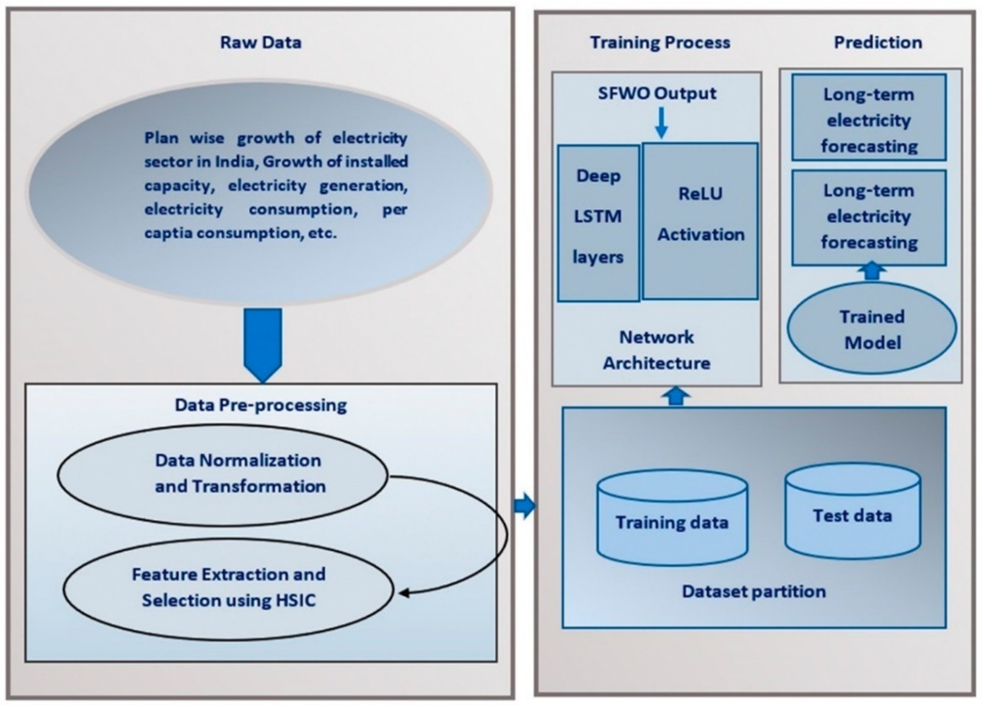
2. Proposed Sailfish Whale Optimization-Based Deep LSTM Approach for Power Generation Forecasting

The surge in electricity consumption necessitates the forecasting of energy demand. Therefore, an electricity demand forecasting model SWO-based Deep LSTM is developed in this study. The proposed approach performs the forecasting process through various phases such as data transformation, technical indicators’ extraction, feature selection, and electricity demand forecasting, as it is shown in Figure 2. Initially, the input time series data is subjected to data transformation phase, where the data is transformed by Box-Cox transformation. However, the technical indicators such as EMA, SMI, CMO, ATR, SMA, CLV, CCI, and OBV are effectively extracted, and the features are selected using HSIC. Finally, the electricity demand forecasting is carried out using a Deep LSTM classifier, trained by the proposed SWO algorithm. The proposed SWO is a combination of SFO [48] and WOA [49]. Figure 2 portrays the schematic diagram of the proposed approach.

Figure 2. Schematic diagram of the proposed SWO-based Deep LSTM for power generation forecasting.

2.1. Acquisition of the Input Time-Series Data

The forecasting of power generation or electricity demand using time series data is performed. Time series data is the data collected at various periods at different points. Data is collected from data.gov.in (23 December 2021). The plan wise growth of electricity sector in India is downloaded which contains the utilities like installed capacity, number of villages electrified, length of T&D lines and per capita energy consumption. The different annual data plans are collected with varying time periods. The plan-wise and category wise growth of various utilities under different modes like hydro, coal/lignite, gas, diesel, nuclear and total values are extracted. Also, the power supply position energy wise and peak wise are considered from 1985 to 2018.

Let us consider the dataset as $S$ with p number of time series data which are mathematically modeled in Equation (1) as,

$$S = \left\{R_n\right\};n \in \left\{1,2,\dots ,p\right\}$$

(1)

where p denotes the total number of data, R represents the time series data, and $R_n$ indicates the data located at $nth$ index of dataset such that the data $R_n$ is used to perform the forecasting process of electricity demand.

Figure 3 shows the architecture diagram of the SWO Deep LSTM model. The preprocessed data is fed to the model with the network architecture of stacked/Deep LSTM layers with ReLU activation function. The model is trained and tested for long term prediction of electricity demand forecasting.

Figure 3. Architecture diagram of Proposed SWO Deep LSTM.

2.2. Data Preprocessing and Feature Extraction

The real-world datasets collected may lead to error due to inconsistency. So, it is necessary to preprocess the data for further analysis. There exist various preprocessing techniques that handles messy data. Cosine similarity is computed between the vectors for data normalization. The number of columns in the data are retrieved and are returned into the respective output variables. The data columns are converted into numbers and the entire table is converted to matrix by iterating over each column. If any of the record cannot be converted to a number format, the entire column is returned as a charArray. The attributes are specified as param-value pairs and the parameter values are not case-sensitive. Technical analysis tool is used for extracting and calculating the various technical indicators for further processing. Technical analysis is used for forecasting the future values based on the history of data.

2.3. Data Transformation Using Box-Cox Transformation

The scaling of attributes is done using data transformation. Data reduction strategies are used for removing the redundancies in the dataset and to reduce the number of attributes. To avoid the bias during training process, data should be normalized using Min-Max scaler. The input time series data $R_n$ is subjected to data transformation phase. In this phase, the data transformation occurs by following Box-Cox transformation [50] which is used for measuring the central tendency values represented as in Equations (1)–(30). Data transformation is the process of preparing data effectively prior to performing the forecasting process. This procedure is used to transform the data from one form to another to obtain the most accurate forecasting result. Box-Cox belongs to the power transformation family, where the transformed values are monotonic functions of time series data. However, the Box-Cox transformation is performed by considering the discontinuity at and is expressed as in Equation (2).

$$B_n=\left\{\begin{array}{l}\frac{R_n^{\delta }-1}{\delta };\delta \ne 0\\ \log R_n;\delta =0\end{array}\right.$$

(2)

where $R_n$ specifies the input time series data, $\delta$ signifies the transformation parameter, and $B_n$ represents the outcome of data transformation.

2.4. Extraction of Technical Indicators

The output $B_n$, obtained from the data transformation process, is then fed to the technical indicators’ extraction phase. During this phase, technical indicators such as SMA, EMA, SMI, CMO, CLV, ATR, OBV, and CCI [51] are effectively extracted to achieve optimal prediction results for power generation. The technical indicators are extracted based on historical time-series data. Moving average is calculated using convolution operation. The shift for the upper and lower bounds are calculated where shift indicates the standard deviation of the data. However, the extracted technical indicators are briefly described as follows:

SMA: It is computed by dividing the total price values over $d$ instant time period such that the technical SMA indicator is expressed as in Equation (3).

$$T_1=\frac{{{\displaystyle \sum }}_{j=1}^{d}C}{d}$$

(3)

where, $d$ indicates the time period, and $C$ specifies the stock prices.

EMA: It provides high importance to current values and is calculated based on the recent samples of the time window. EMA is expressed as in Equation (4).

$$T_2=T_2\left(d-1\right)+\frac{2}{\left(d+1\right)}C\left(d\right)$$

(4)

where $\left(d-1\right)$ indicates the prices on the previous day.

SMI: It is the refinement of a stochastic oscillator and is considered the most reliable indicator with limited false swings. It computes the distance between the recent closing prices and relates it to the median of low or high range of values. Accordingly, the SMI technical indicator is represented using Equation (5) given below.

$$T_3=100\times \frac{M}{\frac{H}{2}}$$

(5)

Here, the terms $H$ and $M$ are specified as in Equations (6) and (7),

$$H=H_1-H_2$$

(6)

$$M=C_{close}-\frac{H}{2}$$

(7)

where $C_{close}$ represents the closed price values, $H_1$ indicates the highest high value, $H_2$ specifies the least low value.

CMO: It is computed by dividing the total movement by the net amount and is expressed in Equation (8) as follows.

$$T_4=100\times {{\displaystyle \sum }}_{j=1}^d{C}_{up}-{{\displaystyle \sum }}_{j=1}^d{C}_{down}$$

(8)

where $C_{up}$ indicates the upward price movement and $C_{down}$ specifies the downward price movement.

CLV: It is used to find whether the issues are closed within the trading range and is represented using Equation (9) given below.

$$T_5=\frac{\left(C_{\mathit{close}}-C_{\mathit{lw}}\right)\left(C_{\mathit{hg}}-C_{\mathit{close}}\right)}{C_{\mathit{hg}}-C_{\mathit{lw}}}$$

(9)

where $C_{lw}$ and $C_{hg}$ are the low and high price values.

ATR: It is the measure of volatility such that a higher ATR value indicates high volatility, and a lower value of ATR specifies low volatility. ATR is represented as in Equation (10).

$$T_6=\frac{T\left(d-1\right)\times \left(d-1\right)+A}{d}$$

(10)

where $A$ indicates true range, $A_{hg}$ specifies true high value, and $A_{lw}$ represents true low value. Here, the term $A$ is specified as, in Equation (11).

$$A=A_{hg}-A_{lw}$$

(11)

OBV: It is the cumulative total of down and up volumes. If a close value is greater than the previous value, then the volume is added to the total value. If the volume is lesser than the previous close value, then the volume is subtracted from the total amount as given in Equation (12).

$$T_7=T_7\left(d-1\right)+/-D$$

(12)

where $D$ indicates the volume.

CCI: It is used to represent the cyclic trading trend and to denote the beginning and ending values. It lies in the range of −100 to 100 and the values outside the range specify the oversold or overbought conditions. CCI indicator is represented as follows in Equation (13).

$$T_8=\frac{C_{tp}-C_{atp}}{0.015\times E}$$

(13)

where, $E$ indicates the mean deviation, $C_{atp}$ represents the typical average price, $C_{tp}$ specifies the typical price value and is represented as in Equation (14).

$$C_{tp}=\frac{C_{close}+C_{lw\left(d\right)}+C_{hg\left(d\right)}}{3}$$

(14)

However, the technical indicators extracted from time-series data are represented as $T$, i.e., $T=\left\{T_i\right\};i\in \left\{1,2,\dots ,8\right\}$, respectively.

2.5. Feature Selection Using Hilbert-Schmidt Independence Criterion (HSIC)

Once the technical indicators are extracted, the optimal features are selected in the feature selection stage. Feature selection is a process in which the best and important features are selected by removing the unimportant features to increase prediction performance. The feature selection process is carried out using HSIC [52] to select the essential features from the extracted technical indicators. The feature selection is done based on the dependency between the attributes. The feature selection can be done in two ways. The first method is building up the catalog of features in an incremental manner known as forward selection and the other way is to remove the irrelevant features from the whole dataset called as backward feature selection process. While applying a linear kernel function, both the techniques are equivalent but backward elimination yields better features.

Let Q denote the whole set of features and Q’ denote the subset of features. Q’ is produced recursively by eliminating the least important features from the original dataset Q. σ denotes the parameter of the data kernel matrix K. The algorithm for the Hilbert Schmidt independence criterion is given below (Algorithm 1).

Algorithm 1: HSIC

Input: Entire set of features Q

Output: An ordered set of features Q’

Q’ ϕ

Repeat

σ ≡

U  argmaxu Σsєu HSIC (σ, Q\{s}), U є Q

Q  Q\U

Q’  (Q’, U)

Until Q = ϕ

The different types of kernels like linear kernel, polynomial, radial basis kernel and graph kernel for HSIC are used. These kernels induce similarity measures on the data and depend on the various assumptions on the dependency between the random variables. The final dataset is constructed based on different annual plans of energy sector with respect to 11 different utilities. HSIC helps in effectively analyzing the dependent and independent features for forecasting electricity generation and consumption.

Let us consider another input data as ${\upsilon }_n$ and perform the data transformation process to extract the technical indicators. The technical indicators extracted as discussed above from the data ${\upsilon }_n$ are represented as $G$. Let us consider $U$ and $V$ be the support of technical indicators $T$ and $G$ which define the joint probability distribution of $\left(T,G\right)$ as $P_{T,G}$. Let $a$ be the separate Reproducing Kernel Hilbert Spaces (RKHS) of the real value functions from $U$ to ${\rm M}$ with universal kernel $l\left(.,.\right)$. Similarly, let $b$ be the separate RKHS of the real value functions from $V$ to ${\rm M}$ with universal kernel $k\left(.,.\right)$. However, the cross-covariance between the elements $a$ and $b$ is given belowin Equation (15).

$$\mathit{cov}\left(\lambda \left(T\right),\rho \left(G\right)\right)=O_{T,G}\left[\lambda \left(T\right),\rho \left(G\right)\right]-O_T\left[\lambda \left(T\right)\right]O_G\left[\rho \left(G\right)\right]$$

(15)

where, $\lambda \in a$, $\rho \in b$, and $O$ denote the expectation functions. The unique operator $N_{T,G}:b\to a$ maps the elements of $b$ to the elements of $a$. However, ${\left(\lambda ,N_{T,G}\left(\rho \right)\right)}_a=\mathit{cov}\left(\lambda ,\rho \right)$ for all $\lambda \in a$ and $\rho \in b$, and this operator is termed as cross-covariance operator. Moreover, the dependence measure between the two technical indicators is specified using the squared Hilbert-Schmidt norm of the cross-covariance operator and is given below in Equation (16).

$$HSIC\left(P_{TG},a,b\right): = \parallel N_{TG}\parallel {}_{\vartheta }^2$$

(16)

If $\parallel N_{TG}\parallel {}_{\vartheta }^2$ is zero, then $\left(\lambda ,N_{TG}\left(\rho \right)\right)$ is always zero for any $\lambda \in a$ and $\rho \in b$. The HSIC is defined using the kernel function and is expressed asin Equation (17).

$$HSIC\left(P_{TG},a,b\right)=O_{T,T^{\prime },G,G^{\prime }}\left[l\left(T,T^{\prime }\right)k\left(G,G^{\prime }\right)\right]+O_{T,T^{\prime }}\left[l\left(T,T^{\prime }\right)\right]O_{G,G^{\prime }}\left[k\left(G,G^{\prime }\right)\right]-O_{T,G}\left[O_{T^{\prime }}\left[l\left(T,T^{\prime }\right)\right]O_{G^{\prime }}\left[k\left(G,G^{\prime }\right)\right]\right]$$

(17)

where $O_{T,T^{\prime },G,G^{\prime }}$ is the expectation over $\left(T,G\right)$ such that $\left(T^{\prime },G^{\prime }\right)$ in which $G$ and $G^{\prime }$ are independently taken from $P_{TG}$. Let ${\rm Y}: = \left\{\left(T_{1,}{G}_1\right),\dots ,\left(T_r,G_r\right)\right\}\subseteq U\times V$ be the collection of $r$ different technical indicators. Accordingly, the estimator of HSIC is represented as in Equation (18).

$$HSIC\left({\rm Y},a,b\right): = {\left(r-1\right)}^{-2}o\left({\rm Z}{\rm X}A{\rm X}\right)$$

(18)

where, $o$ denotes the trace operator, ${\rm Z},{\rm X},A\in {{\rm M}}^{r\times r}$, ${\rm Z}=l\left(T\right)$, $A=k\left(G\right)$, ${\rm X}=I_{r\times r}-r^{-1}{1}_r{1}_r^{ƛ}$, ${\rm X}$ is the centering matrix, $l,k$ are the semi-definite kernel functions, $I_{r\times r}$ represents identity matrix, and $1_r$ is the vector of $r$ ones. To increase the dependence between two technical indicators, the value of the tracing operator must be increased. However, the features selected using HSIC are represented as ${\rm N}$ with the dimensions of $u\times v$, respectively.

3. Forecasting Power Generation Using the Proposed SWO-Based Deep LSTM

The selected feature ${\rm N}$ is used to forecast power generation or electricity demand based on a Deep LSTM classifier. However, the training process of Deep LSTM is carried out using the proposed SWO. SWO is a result of integrating SFO with WOA. The structure of deep CNN and the training procedure of deep learning classifier are described in the below section.

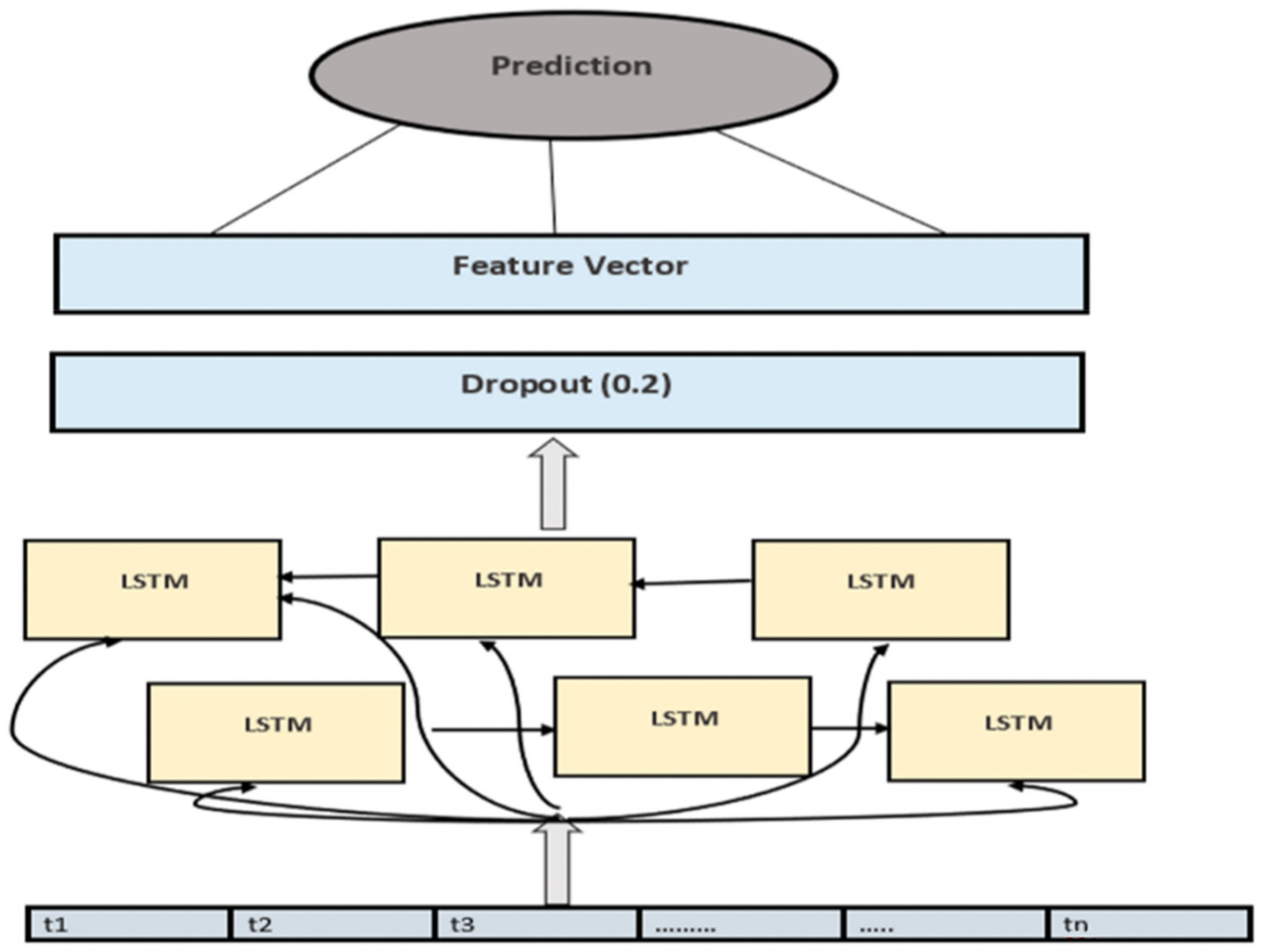
3.1. Structure of Deep LSTM

A deep LSTM classifier is highly effective in performing the forecasting process than the traditional classifiers. This is because only a minimum sample size is required to train the classifier. It can effectively deal with large datasets and works well with a broad range of parameters like learning rate, input, and output gate bias. The input given to the Deep LSTM [53] classifier is ${\rm N}$ which is the optimal feature selected using HSIC. Deep LSTM is used to learn long-term dependencies. Further, it is specified with the input state $f_y$, input gate ${\chi }_y$, forget gate $F{F}_y$, a cell $C{C}_y$, output gate ${\eta }_y$, and the memory unit $Y_y$, respectively. For recurrent neurons at this layer, the memory unit $Y_y$ is computed based on the input ${\rm N}$ and the response $Y_{y-1}$ from the previous time period which are given asin Equation (19).

$$Y_y=\theta \left(Q_{IH}{f}_y+Q_{HH}{Y}_{y-1}+{\alpha }_{\kappa }\right)$$

(19)

where $\theta \left(.\right)$ denotes the activation function, ${\alpha }_{\kappa }$ represents the bias vector, $Q_{IH}$ denotes the weight between input and hidden layers and $Q_{HH}$ specifies the matrix of recurrent weight connected between the hidden layers, which are used to explore the temporal dependency. The input gate ${\chi }_y$ is represented asin Equation (20).

$${\chi }_y=\gamma \left(Q_{a1}{f}_y+Q_{a2}{Y}_{y-1}+Q_{a3}C{C}_{y-1}+{\alpha }_{\chi }\right)$$

(20)

where $Q_{a1}$ represents the weight matrix that is connected between the input state $f_y$ and the input gates ${\chi }_y$. $Q_{a2}$ represents the weight between the memory unit and the input gate, $Q_{a3}$ indicates the weight between cell and the input gate, $\gamma$ specifies the sigmoid function given as $\gamma \left(f_y\right)=\frac{1}{\left(1+e^{-f}\right)}$, and ${\alpha }_{\psi }$ indicates the bias such that $\psi \in \left\{\kappa ,\chi ,FF,CC,\eta \right\}$. However, the input and the forget gate manage the flow of information in the cell. Accordingly, the output gate is used to control how much information is passed from the cell to the memory unit $Y_y$. Moreover, the memory cell is associated with the self-connected recurrent edge with a weight of ‘1’ that ensures to pass the gradient without exploding or vanishing. The forget gate $F{F}_{ y}$ is expressed as in Equation (21).

$$F{F}_y=\gamma \left(Q_{a4}{f}_y+Q_{a5}{Y}_{y-1}+Q_{a6}C{C}_{y-1}+{\alpha }_{FF}\right)$$

(21)

where $Q_{a4}$ represents the weights of input and forget gates, $Q_{a5}$ specifies the weights of the memory unit and forget gate, $Q_{a6}$ indicates the weight between the cell and forget gate, and ${\alpha }_{FF}$ denotes the bias. However, the cell $C{C}_y$ of Deep LSTM is represented as in Equation (22).

$$C{C}_y=F{F}_y\circ C{C}_{y-1}+{\chi }_y\circ \mathit{tan}h\left(Q_{a7}{f}_y+Q_{a8}{Y}_{y-1}+{\alpha }_{CC}\right)$$

(22)

where $\circ$ represents the element-wise product, $Q_{a7}$ indicates the weight between input and the cell, $Q_{a8}$ is the weight between cell and the memory unit and ${\alpha }_{CC}$ is the bias. Finally, the output gate and the output obtained from the memory unit are expressed as in Equations (23) and (24).

$${\eta }_y=\gamma \left(Q_{a9}{f}_y+Q_{a10}{Y}_{y-1}+Q_{a11}C{C}_y+{\alpha }_{\eta }\right)$$

(23)

$$Y_y={\eta }_y\circ \mathit{tan}h\left(C{C}_y\right)$$

(24)

where $Q_{a9}$ denotes the weights of input and output gates, $Q_{a10}$ and $Q_{a11}$ denote the weights of two entities such as memory unit and output gate, as well as between cell and output gates. Moreover, the output obtained from the output layer is expressed asin Equation (25).

$${\mu }_y=\varpi \left(Q_{a12}{Y}_y+{\alpha }_{\mu }\right)$$

(25)

where $Q_{a12}$ specifies the weight between memory unit and output vector, ${\mu }_y$ denotes the output vector, and ${\alpha }_{\mu }$ indicates the bias of output vector.

Figure 4 represents the architecture of Deep LSTM classifier, which provides improved accuracy for prediction using time series datasets with the different gates like input, output and forget gates and the memory unit.

Figure 4. The architecture of a Deep LSTM classifier.

Figure 5 shows the architecture of LSTM that can effectively capture the temporal dependencies in the time series dataset using network loops. LSTM processes the input sequences in the data and is capable of mapping input to output functions effectively.

Figure 5. Temporal data dependency in Deep LSTM model.

Deep LSTM has a greater number of hidden layers with memory cells in each layer. Output is generated at every single step and no single output for all the input steps is generated. Multiple LSTM layers are stacked in more layers which produces deeper high-level representation. In the sequential modeling, the number of hidden layers can be added. The return attribute value is set to zero during modeling. For better optimization results, the previous layers outputs are learned by the higher layers. Deep LSTM selects only the dependent features from the original dataset. Technical analysis tool is used for extracting and selecting the best features for modeling. The output is represented as a vector that produces the predicted values.

3.2. Selection of Nodes and Hyper Parameters for Deep LSTM

The prediction results are obtained depending on the training dataset. Q_k denotes the number of nodes chosen for testing to determine the loss values as in Equation (26).

$$Q_k=\frac{Q_s}{\left(\alpha \ast \left(Q_i+Q_0\right)\right)}$$

(26)

$Q_i$ represents the input neurons, $Q_0$ represents the output neurons and $Q_s$ represents the total number of training samples and $\alpha$ denotes the scaling factor. Based on the estimation of loss values, the optimal model is chosen. 70% of the dataset is taken for training and the remaining 20% for testing. The statistical features like mean and standard deviation are computed for the training samples. The number of features, responses and the number of hidden units are identified for training. Table 3 determines the hyper parameter settings of Deep LSTM model for training the data samples.

Table 3. Input parameters for Deep LSTM.

Input Parameters	Values
Optimizer	Adam
Number of hidden units	200
MaxEpochs	250
Gradient Threshold	1
Initial Learning Rate	0.005
Learn rate schedule	Piece-wise
Learn rate drop period	125
Dropout factor	0.2

The data for different annual plans of energy sector are considered for training and testing.

In order to avoid over-fitting of data, some neurons in the hidden units are not considered. The complex patterns are discovered using deep LSTM model and drop out layers are used to neglect few neurons during the training process. For retaining the accuracy of the model, the drop out layer is added after every LSTM layer and the value of dropout is set to 0.2. For interpreting the output values, the density layer is added after every LSTM layer with the ReLU activation function. Sequence of data points are present in the training samples and last time step output is fed to the next preceding input sequence. Adam optimizer is used, which is an effective optimization algorithm with a smaller number of hyper parameter tuning. Adam optimizer produces good result with minimum loss value than RMSProp optimization [54]. The output of Sailfish Whale Optimization algorithm is fed as input to the Deep LSTM model.

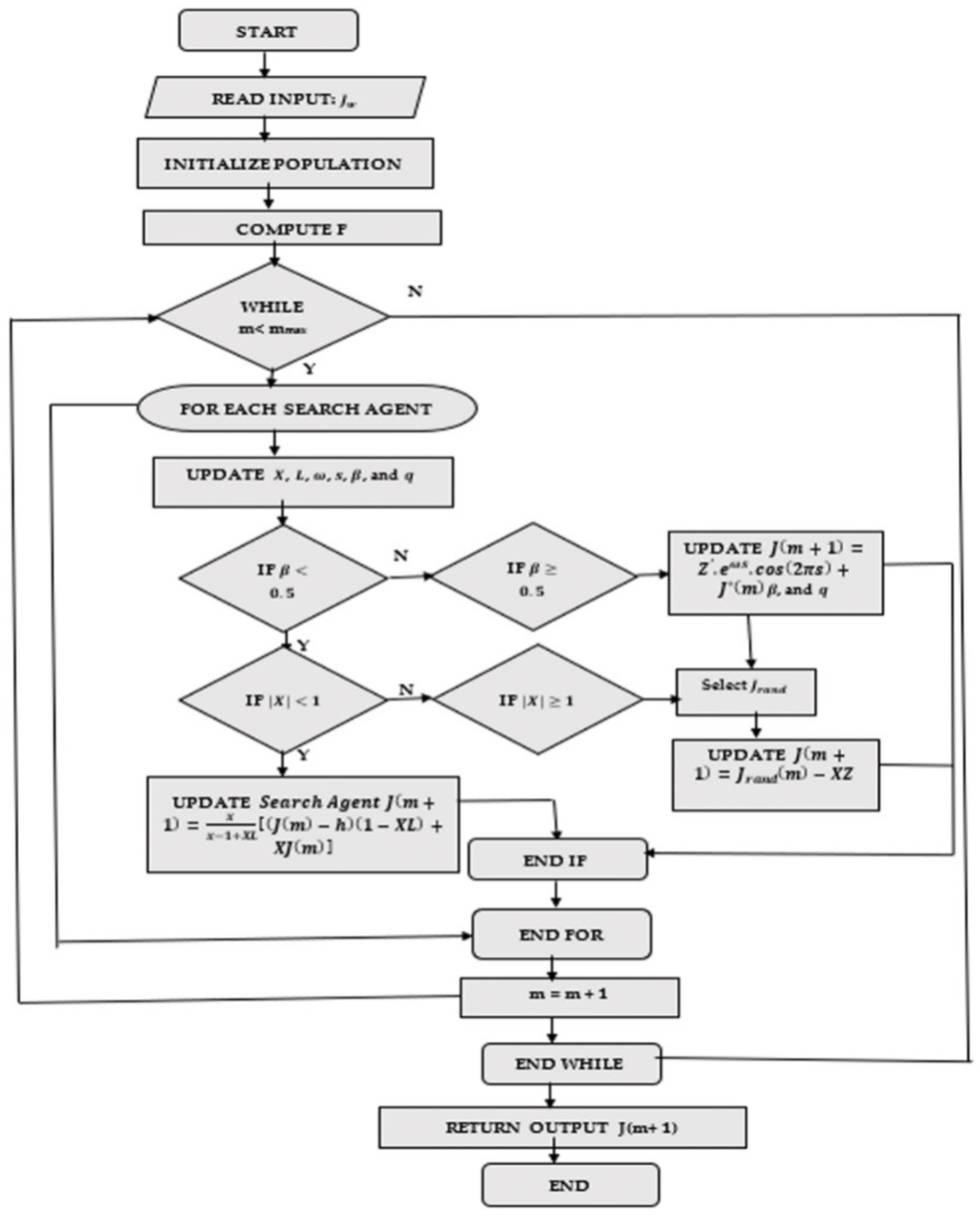
3.3. Proposed Sailfish Optimization Algorithm

The proposed SWO is used to train the Deep LSTM classifier to obtain the best prediction accuracy. Being a meta-heuristic optimization algorithm, WOA mimics the humpback whales’ characteristics. WOA is inspired based on the strategy of the bubble-net hunting mechanism. The major advantage of using WOA is the hunting behavior of whales in chasing the prey and using the spiral model to simulate the bubble net model of humpback whales. SFO is a swarm-based algorithm that was developed based on the inspiration of sailfish’s hunting behavior. SFO contains two population tips namely intensification and diversification of search space. The fastest fish in the ocean, i.e., Sailfish, can reach up to a maximum speed of 100 km per hour. They hunt small fishes called sardines on the surface. The sailfish makes a slashing motion, injures several sardines, taps, and destabilizes the sardine. So, the integration of parametric features, for instance, hunting behavior and the foraging behavior of humpback whales and sailfish increase the performance of forecasting power generation. The algorithmic steps of the proposed SWO are explained in Figure A1 (Appendix A). Equations (A1)–(A22) are included in the Appendix A section.

(i) Initialization: Let us initialize the whales’ population as $\delta$ with $c$ number of humpback whales $J$ which is expressed as in Equation (A1).

(ii) Compute the fitness function: The fitness measure is used to compute the best solution to forecast the energy demand and is expressed as in Equation (A2), where $F$ is the fitness, $\aleph$ indicates the total number of samples, and ${\Re }^{\nu }$ is the estimated output.

(iii) Update the parameters $X$, $L$, $\omega$, $s$, $\beta$ and $q$: Let us specify the parameters $X$ and $L$ as vectors, s and $\beta$ as random numbers, and $\omega$ as the constant term. However, the vector $X$ and $L$ are computed as followsin Equations (A3) and (A4), where, $q$ gets linearly decreased from 2 to 0 with respect to iterations, and $z$ denotes a random vector that ranges in the interval of $\left[0,1\right]$. Here, random numbers $s$ and $\beta$ are in the interval range of $\left[-1,1\right]$ and $\left[0,1\right]$, respectively.

(iv) Update spiral position: The spiral equation is generated between the location of prey and whale to mimic the helix-shaped movement of whales which is expressed as in Equation (A5), where $Z^{\prime }=\left|J^{*}\left(m\right)-J\left(m\right)\right|$ denotes the distance between the whale and the prey, $\omega$ represents the constant, $s$ indicates the random number, and $‘.’$ specifies element-by-element multiplication.

(v) Search for prey: During the exploration phase, every search agent’s position is updated based on randomly selected search agent rather than the best one. However, the update process at exploration phase is given as follows in Equations (A6) and (A7).

(vi) Update the position of search agent: The humpback whales find the location of prey and encircle it. The encircling behavior is used to update the position of search agent towards the best agent and is mathematically expressed as in Equations (A8)–(A13) by assuming $J^{*}\left(m\right)>J\left(m\right)$. The standard equation of SFO is expressed as in Equations (A14)–(A16).

(vii) Final update equation: The final update equation is obtained by substituting Equation (A15) in Equation (A12) and is expressed as in Equations (A17)–(A22), where $m$ specifies the current iteration, $X$ and $L$ are the vectors, $x$ denotes the random number in the range of 0 to 1, and $h$ denotes the attack power of sailfish at each iteration and is represented asin Equation (A22), where, $g$ and $t$ are the coefficients that reduce the value of power attack from $g$ to 0.

(viii) Termination: The above steps are repeated until a better solution is obtained in the search space.

Figure A1 (Appendix A) portrays the flow chart of the proposed SWO-based Deep LSTM.

3.4. Experimental Setup and Dataset Description

The proposed approach is implemented using MATLAB software tools using a real-time dataset. The data was collected from data.gov.in [55] (Central Electricity Authority, Government of India, 2019, accessed on 31 March 2021). Here, 11 different utilities are considered to predict the energy requirements for the future. The 11 different utilities considered in this study are install capacity prediction, the number of villages electrified prediction, length of T&D lines prediction, hydro prediction, coal prediction, gas prediction, diesel, nuclear, total, renewable energy source, and total prediction. The real-time data was observed from the digital source of data.gov.in (23 December 2021). With these utilities, the energy required for the future was predicted using various methods, along with the proposed SWO-based Deep LSTM approach.

3.5. Inspection of Model Quality

The goodness of the model used for the prediction of electricity demand is analyzed using different evaluation metrics like Mean Squared Error (MSE), Root Mean Squared Error (RMSE), normalized Mean Squared Error (nMSE), and normalized Root Mean Squared Error (nRMSE).

3.5.1. Mean Squared Error (MSE)

MSE is the difference between the actual value and the predicted value. It is extracted by squaring the MSE of the dataset as in Equation (27).

$$MSE=\frac{1}{\aleph }{{\displaystyle \sum }}_{\nu =1}^{\aleph }{\left[W_{\nu }-R_v\right]}^2$$

(27)

where $\aleph$ denotes the total number of samples, $W$ denotes the actual value, and $R$ indicates the predicted value.

3.5.2. Root Mean Squared Error (RMSE)

RMSE is the standard deviation of the prediction errors or residuals. It is denoted as in Equation (28).

$$RMSE=\sqrt{\frac{1}{\aleph }{{\displaystyle \sum }}_{\nu =1}^{\aleph }{\left[W_{\nu }-R_v\right]}^2}$$

(28)

where $\aleph$ denotes the total number of samples, $W$ denotes the actual value and $R$ indicates the predicted value.

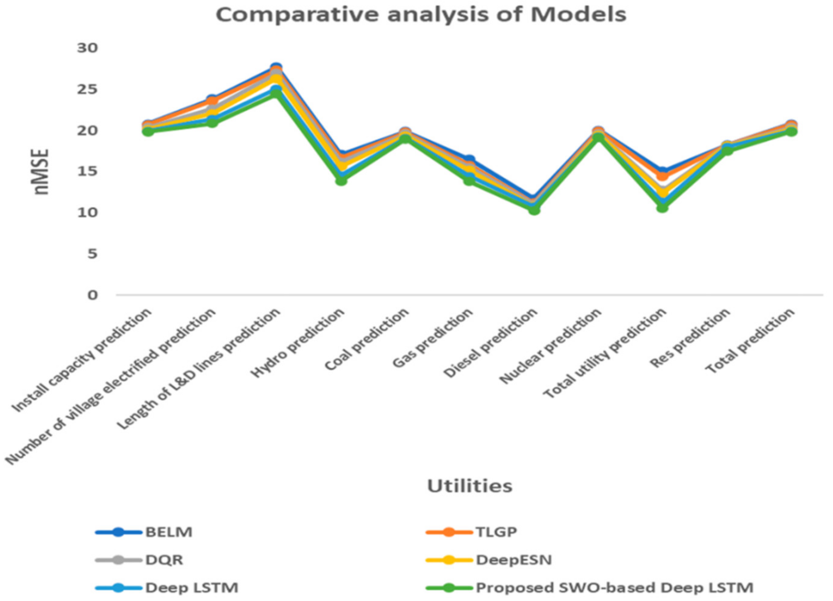
3.5.3. Normalized Mean Squared Error (nMSE)

The normalized Mean Square Error (nMSE) statistic highlights the scatter in the whole dataset, and NMSE will not be biased towards the models that under-predict or over-predict. Lower NMSE values denote the better performance of the model. NMSE is denoted as in Equation (29).

$$nMSE=\frac{\overline{{\left(W_v-R_v\right)}^2}}{\overline{W_v}X\overline{R_v}}$$

(29)

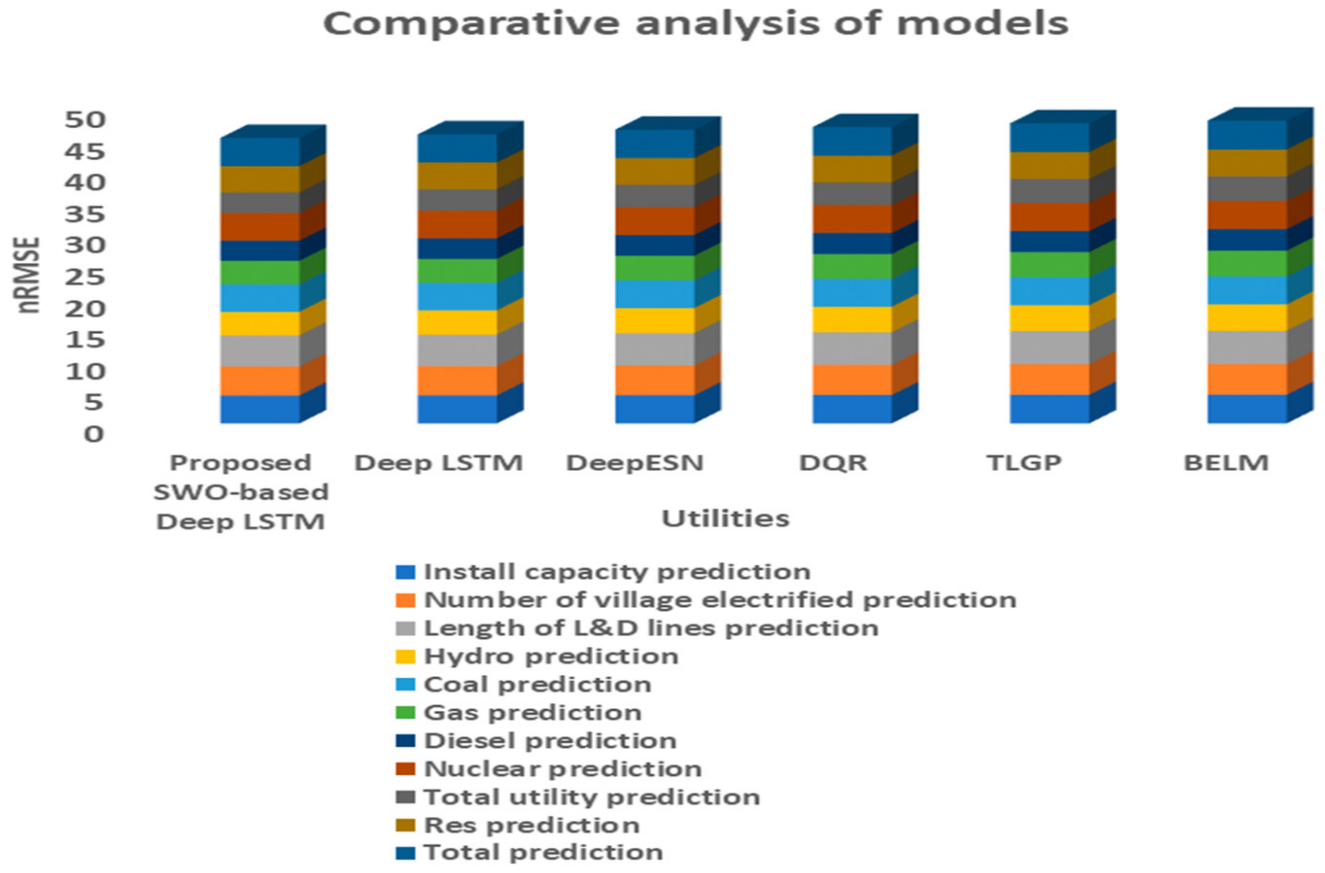
3.5.4. Normalized Root Mean Squared Error (nRMSE)

The normalized RMSE is interpreted as a fraction of the overall range that is resolved by the model. It is used to relate the RMSE to the observed range of the variable as in in Equation (30).

$$NRMSE=\frac{RMSE}{\aleph }$$

(30)

where $\aleph$ denotes the total number of samples, $W$ denotes the actual value and $R$ indicates the predicted value.

4. Results and Discussion

This section presents the results and discussions for the proposed SWO-based Deep LSTM based on the predictions.

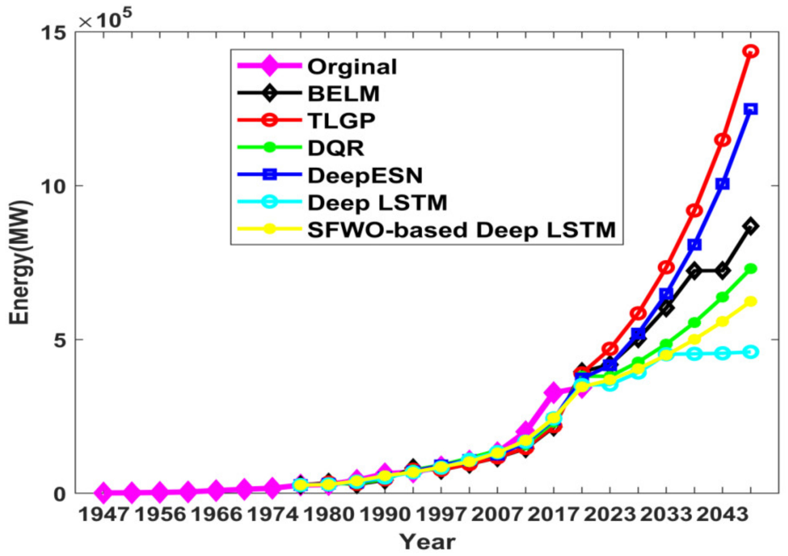
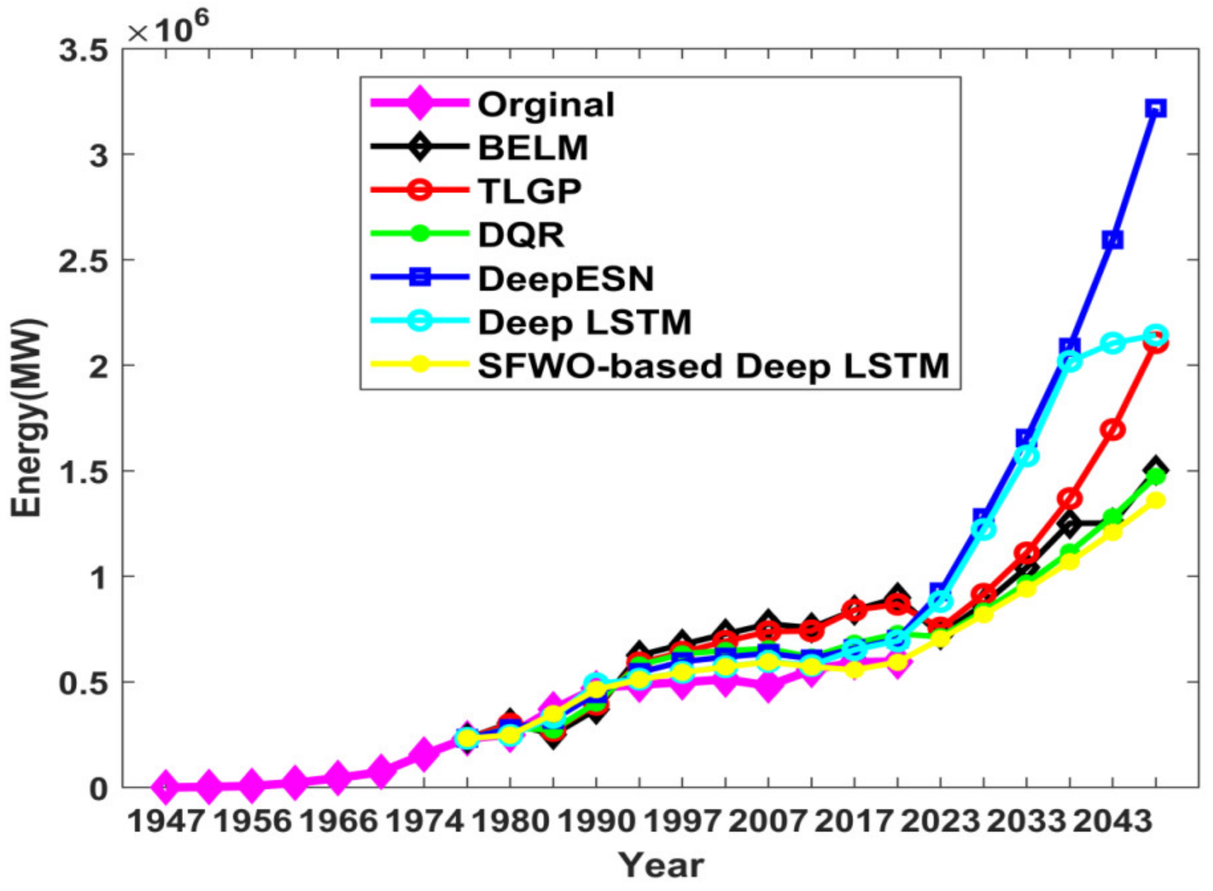
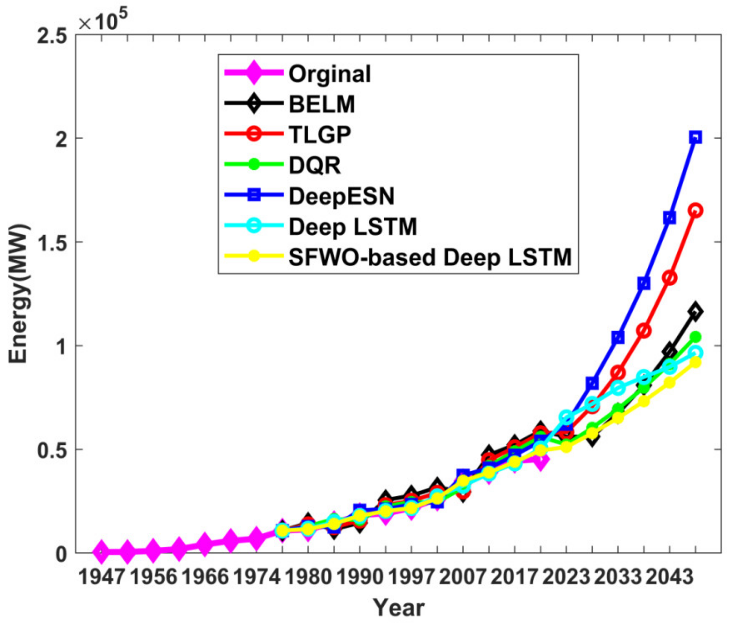
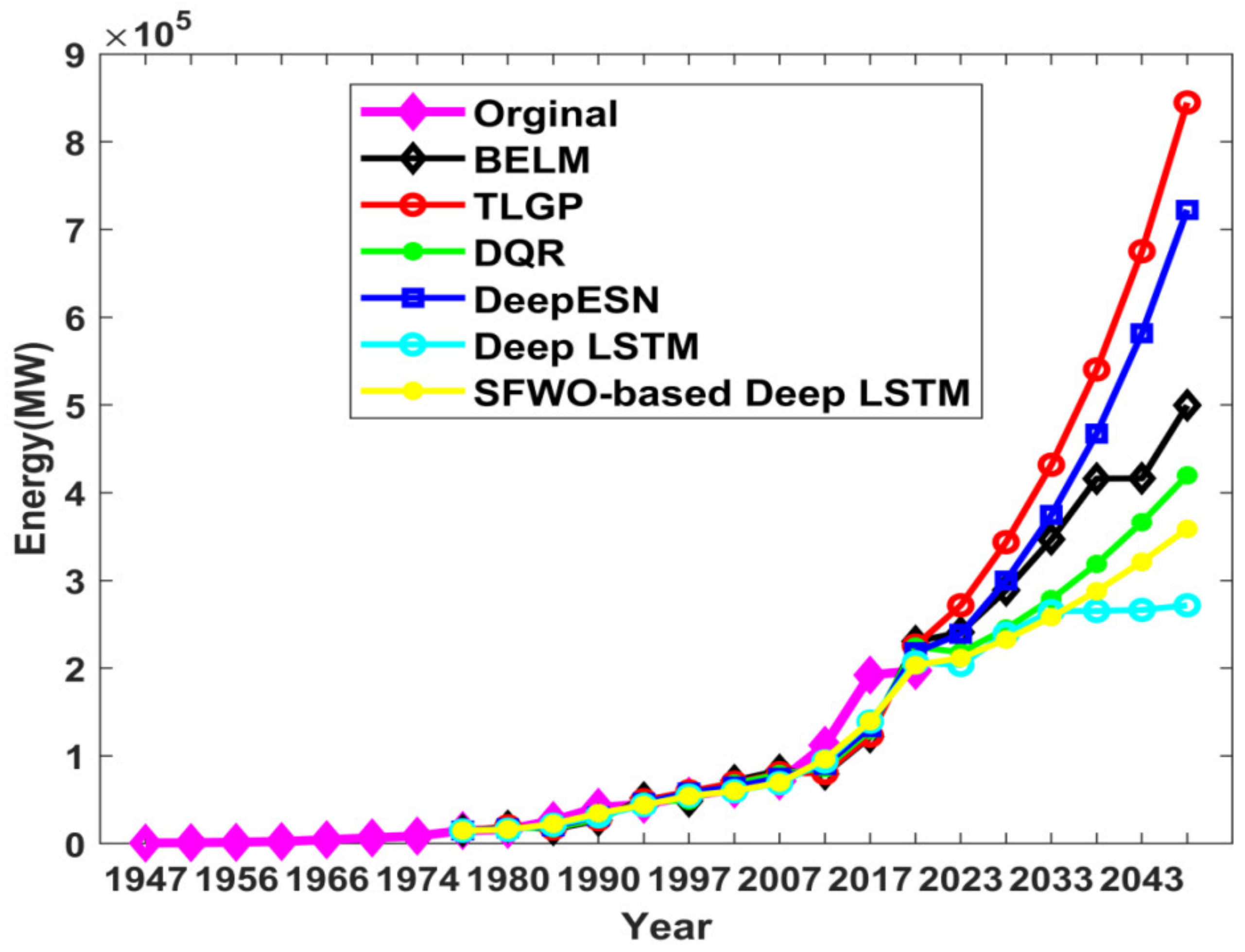
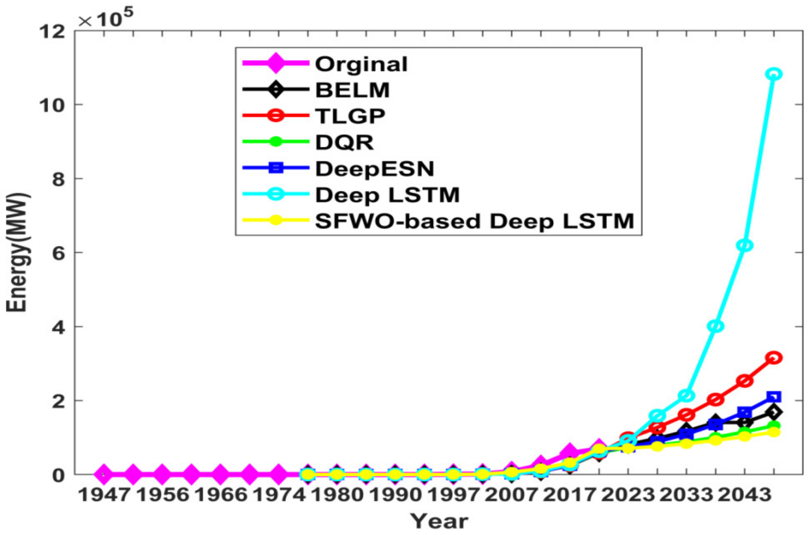
4.1. Comparative Analysis of Energy Prediction

The existing methods used to compare the performance of the proposed model are Bootstrap-based ELM approach (BELM) [21], Direct Quantile Regression (DQR) [42], Temporally Local Gaussian Process (TLGP) [24], Deep Echo State Network (Deep ESN) [47] and Deep LSTM [45].

This section details the comparative analyses of the proposed SWO-based Deep LSTM for energy prediction until the year 2048.

(a) Comparative analysis of install capacity prediction

Figure 6 depicts the install capacity prediction of the proposed approach. In the year 2018, the original energy was 344.00 GW, whereas the energy prediction outcome using existing techniques such as BELM, TLGP, DQR, Deep ESN, Deep LSTM, and the proposed SWO-based Deep LSTM are 373.10 GW, 394.98 GW, 351.87 GW, 381.01 GW, 389.56 GW and 345.83 GW. The error between the original energies with respect to prediction outputs using BELM, TLGP, DQR, Deep ESN, Deep LSTM, and the proposed SWO-based Deep LSTM were 29.10 GW, 50.98 GW, 7.87 GW, 37.01 GW, 45.56 GW, and 1.83 GW, respectively. The above inference shows that the proposed method yielded better performance than the existing method due to the improved training of the proposed model.

Figure 6. Comparative analysis of proposed SWO-DLSTM model for install capacity prediction.

(b) Comparative analysis of the village electrified prediction

Figure 7 shows the number of villages electrified prediction based on the proposed approach. In the year 2018, the original energy was 597.121 GW, whereas the energy prediction outcome using existing techniques such as BELM, TLGP, DQR, Deep ESN, Deep LSTM, and the proposed SWO-based Deep LSTM were 593.58 GW, 728.54 GW, 702.69 GW, 898.60 GW, 867.900 GW, and 694.50 GW.

Figure 7. Comparative analysis of proposed SWO-DLSTM model for village electrified prediction.

The error between the original energies with respect to prediction outputs using BELM, TLGP, DQR, Deep ESN, Deep LSTM, and the proposed SWO-based Deep LSTM were 3.536 GW, 131.42 GW, 105.57 GW, 301.48 GW, 270.77 GW, and 97.37 GW, respectively. From the above inference, the study proves that the proposed method achieved better performance than the existing methods.

(c) Comparative analysis of the length of the L&D lines prediction

Figure 8 depicts the length of L&D lines prediction of the proposed approach. In the year 2018, the original energy was 11,031.059 GW, whereas the energy prediction outcomes using existing techniques such as BELM, TLGP, DQR, Deep ESN, Deep LSTM, and the proposed SWO-based Deep LSTM were 12,759,557.62 MW, 13,157.239 GW, 11,997.569 GW, 13,965.28 GW, 13,598.33 GW, and 11,809.26 GW.

Figure 8. Comparative analysis of proposed SWO-DLSTM model for length of L&D lines utility prediction.

The error between the original energies with respect to prediction outputs using BELM, TLGP, DQR, Deep ESN, Deep LSTM, and the proposed SWO-based Deep LSTM were 1728.498 GW, 2126.180 GW, 966.510 GW, 2934.227 GW, 2567.279 GW, and 778.210 GW, respectively. Due to the performance of the proposed optimization algorithm in deep learning, the training capability of the method is highly improved and has obtained much better results compared to the existing algorithms.

(d) Comparative analysis of the hydro prediction

Figure 9 depicts the hydro prediction of the proposed approach. In the year 2018, the original energy was 45.293 GW, whereas the energy prediction outcomes using existing techniques such as BELM, TLGP, DQR, Deep ESN, Deep LSTM, and the proposed SWO-based Deep LSTM were 53.91 GW, 56.03 GW, 50.45 GW, 58.87 GW, 57.71 GW, and 49.44 GW. The error between the original energies with respect to prediction outputs using BELM, TLGP, DQR, Deep ESN, Deep LSTM, and proposed SWO-based Deep LSTM were 8.62 GW, 10.73 GW, 5.16 GW, 13.58 GW, 12.42 GW, and 4.14 GW respectively.

Figure 9. Comparative analysis of proposed SWO-DLSTM model for hydro utility prediction.

(e) Comparative analysis of the coal prediction

Figure 10 portrays the coal prediction of the proposed approach. In the year 2018, the original energy was 197.17GW, whereas the energy prediction outcome using existing techniques such as BELM, TLGP, DQR, Deep ESN, Deep LSTM, and the proposed SWO-based Deep LSTM were 218.01 GW, 225.63 GW, 206.56 GW, 224.39 GW, 230.44 GW, and 203.36 GW.

Figure 10. Comparative analysis of proposed SWO-DLSTM model for coal utility prediction.

The error between the original energies with respect to prediction outputs using BELM, TLGP, DQR, Deep ESN, Deep LSTM, and the proposed SWO-based Deep LSTM were 20.84 GW, 28.46 GW, 9.38 GW, 27.22 GW, 33.27 GW, and 6.19 GW, respectively.

(f) Comparative analysis of the gas prediction

Figure 11 depicts the gas prediction of the proposed approach. In the year 2018, the original energy was 24.89W, whereas the energy prediction outcomes using existing techniques such as BELM, TLGP, DQR, Deep ESN, Deep LSTM, and the proposed SWO-based Deep LSTM were 29.005 GW, 31.45 GW, 27.472 GW, 29.97 GW, 37.51 GW, and 26.99 GW. The error between the original energies with respect to prediction outputs using BELM, TLGP, DQR, Deep ESN, Deep LSTM, and proposed SWO-based Deep LSTM were 4.108 GW, 6.553 GW, 2.575 GW, 5.077 GW, 12.62 GW, and 2.097 GW, respectively.

Figure 11. Comparative analysis of proposed SWO-DLSTM model for gas utility prediction.

(g) Comparative analysis of the diesel prediction

Figure 12 depicts the diesel prediction of the proposed approach. In the year 2018, the original energy was 0.838GW, whereas the energy prediction outcomes using existing techniques such as ELM, TLGP, DQR, Deep ESN, Deep LSTM, and the proposed SWO-based Deep LSTM were 0.867 GW, 1.221 GW, 1.006 GW, 1.192 GW, 1.322 GW, and 0.973 GW.

Figure 12. Comparative analysis of proposed SWO-DLSTM model for diesel utility prediction.

The error between the original energies with respect to prediction outputs using BELM, TLGP, DQR, Deep ESN, Deep LSTM, and proposed SWO-based Deep LSTM were 0.0298 GW, 0.383 GW, 1.68 GW, 0.354 GW, 0.484 GW and 0.135 GW respectively.

(h) Comparative analysis of the nuclear prediction

Figure 13 portrays the nuclear prediction of the proposed approach. In the year 2018, the original energy was 6.780GW, whereas the energy prediction outcomes using existing techniques such as BELM, TLGP, DQR, Deep ESN, Deep LSTM, and the proposed SWO-based Deep LSTM were 248.80GW, 259.49 GW, 235.11 GW, 255.20 GW, 248.58 GW, and 231.24 GW. The error between the original energies, with respect to prediction outputs using BELM, TLGP, DQR, Deep ESN, Deep LSTM, and the proposed SWO-based Deep LSTM were 242.022 GW, 252.71 GW, 228.33 GW, 248.42 GW, 241.80 GW and 224.46 GW, respectively.

Figure 13. Comparative analysis of proposed SWO-DLSTM model for nuclear utility prediction.

(i) Comparative analysis of the total utility prediction

Figure 14 depicts the total prediction of the proposed approach. In the year 2018, the original energy was 222.90GW, whereas the energy prediction outcomes using existing Deep LSTM were 8.30 GW, 7.42 GW, 8.28 GW, 10.18 GW, 7.30 GW.

Figure 14. Comparative analysis of proposed SWO-DLSTM model for total utility prediction.

The error between the original energies with respect to prediction outputs using TLGP, DQR, Deep ESN, Deep LSTM, and the proposed SWO-based Deep LSTM were 214.59 GW, 215.48 GW, 214.61 GW, 212.72 GW and 215.59 GW respectively.

(j) Comparative analysis of the Renewable Energy Source (RES) prediction

Figure 15 depicts the Renewable Energy Source (RES) prediction of the proposed approach. In the year 2018, the original energy was 69.022 GW, whereas the energy prediction outcomes using existing techniques such as BELM, TLGP, DQR, Deep ESN, Deep LSTM, and the proposed SWO-based Deep LSTM were 62.14 GW, 69.89 GW, 58.69 GW, 59.11 GW, 63.23 GW, and 57.95 GW. The error between the original energies with respect to prediction outputs using BELM, TLGP, DQR, Deep ESN, Deep LSTM, and the proposed SWO-based Deep LSTM were 6.87 GW, 8.73 GW, 10.32 GW, 9.90 GW, 5.78 GW, and 11.06 GW, respectively.

Figure 15. Comparative analysis of proposed SWO-DLSTM model for RES prediction.

(k) Comparative analysis of the total prediction

Figure 16 represents the total prediction of the proposed approach. In the year 2018, the original energy was 344.002 GW, whereas the energy prediction outcomes using existing techniques such as BELM, TLGP, DQR, Deep ESN, Deep LSTM, and the proposed SWO-based Deep LSTM were 373.10 GW, 394.98 GW, 351.87 GW, 381.05 GW, 389.564 GW, and 345.83 GW. The error between the original energies with respect to prediction outputs using BELM, TLGP, DQR, Deep ESN, Deep LSTM, and the proposed SWO-based Deep LSTM were 29.10 GW, 50.98 GW, 7.87 GW, 37.01 GW, 45.56 GW, and 1.83 GW, respectively.

Figure 16. Comparative analysis of proposed SWO-DLSTM model for total prediction.

4.2. Research Results and Outcome Analysis

For effective research outcomes, the proposed model has been tested for different facility predictions and recorded the best fitness and mean fitness. In order to prove the efficiency of the proposed model, the results of the SWO-Deep LSTM are compared with the various existing models like bootstrap-based ELM, Deep Echo state network, TLGP, DQR and Deep LSTM.

While analyzing the behavior of ELM, the prediction accuracy of the model is improved by selecting the most important neurons that have an impact on the structure of the neural network and thereby reducing the over-fitting of data. The optimal set of neurons are chosen based on the restructuring and re-sampling techniques by applying a pruning method. The neuron shrinkage technique is used in the ELM based on the bootstrap replications. The stability of the model selection is improved with the use of the re-sampling technique through bootstrapping. Although ELM is faster in the training phase, it does not provide precise and accurate results for non-linear data. To handle highly non-linear data approximation, the Deep Neural Networks provide improved accuracy. In Table 4 and Table 5, the normalized MSE and normalized RMSE values of the different facility prediction bootstrap-based ELM are poor compared to the other methods.

Table 4. Comparative table for normalized MSE.

Prediction	BELM [21]	TLGP [24]	DQR [42]	Deep ESN [47]	Deep LSTM [45]	Proposed SWO-Based Deep LSTM
Install capacity prediction	20.792	20.697	20.395	20.129	19.938	19.855
Number of village electrified prediction	23.830	23.589	22.622	22.076	21.380	20.868
Length of L&D lines prediction	27.720	27.327	26.949	26.329	25.054	24.415
Hydro prediction	17.094	16.650	16.168	15.664	14.523	13.855
Coal prediction	19.889	19.784	19.583	19.374	19.049	18.975
Gas prediction	16.495	15.777	15.494	15.155	14.446	13.821
Diesel prediction	11.712	11.182	11.066	10.821	10.759	10.309
Nuclear prediction	20.045	19.950	19.657	19.455	19.234	19.149
Total utility prediction	15.083	14.368	12.756	12.420	11.319	10.579
Res prediction	18.246	18.227	18.207	18.168	18.020	17.467
Total prediction	20.791	20.698	20.398	20.128	19.936	19.853

Table 5. Comparative table for normalized RMSE.

Prediction	BELM [21]	TLGP [24]	DQR [42]	Deep ESN [47]	Deep LSTM [45]	Proposed SWO-Based Deep LSTM
Install capacity prediction	4.5598	4.5494	4.5161	4.4865	4.4652	4.4559
Number of village electrified prediction	4.8816	4.8568	4.7562	4.6985	4.6238	4.5682
Length of L&D lines prediction	5.2650	5.2276	5.1913	5.1312	5.0054	4.9411
Hydro prediction	4.1345	4.0804	4.0210	3.9578	3.8109	3.7222
Coal prediction	4.4597	4.4479	4.4253	4.4016	4.3645	4.3561
Gas prediction	4.0615	3.9720	3.9362	3.8929	3.8008	3.7177
Diesel prediction	3.4223	3.3440	3.3266	3.2896	3.2801	3.2108
Nuclear prediction	4.4772	4.4665	4.4336	4.4107	4.3856	4.3760
Total utility prediction	3.8837	3.7906	3.5715	3.5242	3.3643	3.2526
Res prediction	4.2715	4.2693	4.2670	4.2623	4.2450	4.1794
Total prediction	4.5599	4.5496	4.5163	4.4864	4.4653	4.4558

The TLGP is used to estimate the forecasting uncertainty with the analytical interval forecasting framework. The local window is defined where the data in the local window is used for prediction. Instead of maximum likelihood techniques, the least squared technique is used to optimize the hyperparameters. Using TLGP, the learning procedure is global, and the prediction process is local. Compared with the Gaussian process, the computational complexity of the learning and inference stage is reduced using TLGP. TLGP generates residuals that are like Gaussian and is understood through the statistical error analysis. For the limited amount of data, TLGP shows the higher prediction uncertainty for one-step forecasting. Since the training data is moved forward in the time domain, the error values of the different facility predictions are better than the ELM technique, as shown in Table 4 and Table 5. The accuracy is reduced when the size of the dataset increases.

The Direct Quantile Regression technique combines extreme machine learning and regression for non-parametric probabilistic forecasting of power generation. The conditional densities using the quantile regression technique are described. The quantile of the response variable is estimated as the function of input variables. The quantile regression can provide only the description of a particular quantile. The distribution shape assumes, and the main problem is the lack of information about uncertainty present in the quantile. At a time, a single quantile function can be estimated, and it provides reasonable accuracy for the smaller datasets and fails to perform well when the training dataset is increased. For the energy demand forecasting of different facility prediction, this technique performs better than the ELM and TLGP as shown in Table 4 and Table 5.

A hybrid approach of LSTM and Echo State Network (ESN) provides good prediction results for energy forecasting. LSTM performs best for handling time-series datasets and the forecasting process involves training of a hidden layer using one epoch and using the regression at the output layer. To achieve the target outcome, quantile regression is used in the echo state network. This approach provides good accuracy with fewer epochs where one epoch is used for training input and output layers and another epoch for fine-tuning operation. Although this model can capture the temporal dependencies in the data, for the increased number of epochs, the accuracy is decreased. This model provides better performance than the ELM, TLGP and DQR methods in forecasting the different facilities of energy prediction.

The deep LSTM model excels in short-term as well as medium-term forecasting of energy demand and efficiently handles big data processing. The model can capture complex patterns easily. The stability of the network is increased by stacking the multiple LSTM layers and increasing the number of neurons in the hidden layer. The number of epochs and the learning rate is set for achieving the minimum normalized RMSE value. The energy demand prediction for different facility using Deep LSTM achieves lower nRMSE values as shown in Table 4 and Table 5 when compared to the other models through efficient data processing and feature extraction techniques. To improve the accuracy of the Deep LSTM model, the feature extraction techniques can be integrated with the model. A hybrid approach can still lead to better performance.

For achieving the optimal solution, the proposed model combines the sailfish whale optimization and the Deep LSTM model. The best search space is updated using the optimization algorithm where the search occurs in a hyper-dimensional space with variable position vectors. Through the location update, the good fittest solutions are retained, and, in each iteration, the best position is saved. This optimization algorithm prevents the local optimum solution and works well for large-scale global optimization. After the maximum number of iterations, the best search space is chosen where the selected features are given as input to the Deep LSTM model to improve the accuracy. As shown in Table 4 and Table 5, the proposed model achieved lower nMSE and lower nRMSE values when compared to the other models for the different energy facility predictions.

Table 4 represents the comparative table for MSE values. The table shows the average MSE value obtained by the existing approaches and the proposed approach. By considering hydro prediction, the normalized MSE values obtained by the existing energy utilized by the prediction techniques such as BELM, TLGP, DQR, Deep ESN, Deep LSTM, and the proposed SWO-based Deep LSTM were 17.094, 16.650, 16.168, 15.664, 14.523, and 13.855, respectively. When taking diesel prediction into account, the normalized MSE values obtained by existing energy, utilized by the prediction techniques such as BELM, TLGP, DQR, Deep ESN, Deep LSTM and the proposed SWO-based Deep LSTM were 11.712, 11.182, 11.066, 10.821, 10.759, and 10.309, respectively.

Figure 17 shows the analysis of different utilities of models with respect to normalized MSE values. The proposed model achieves percentage improvements of 26%, 21%, 16%, 12% and 6% in terms of Root Mean Squared Error compared with the other existing models. The integration of optimization algorithm and Deep LSTM achieves good accuracy in different utility predictions that helps to attain the effective utilization of energy resources at the distribution systems.

Figure 17. Comparative analysis of nMSE values for different models.

Table 5 represents the comparative analysis for RMSE. The table shows the average RMSE values obtained by the existing approaches and the proposed approach. By considering install capacity prediction, the normalized RMSE values obtained by the existing techniques such as BELM, TLGP, DQR, Deep ESN, Deep LSTM, and the proposed SWO-based Deep LSTM were 74.5598, 4.5494, 4.5161, 4.4865, 4.4652, and 4.4559, respectively. In coal prediction, the normalized RMSE value obtained by the existing techniques such as BELM, TLGP, DQR, Deep ESN, Deep LSTM and the proposed SWO-based Deep LSTM were 4.4597, 4.4479, 4.4253, 4.4016, 4.3645, and 4.3561 respectively.

Figure 18 shows the analysis of different utilities of models with respect to normalized RMSE values. The proposed model achieves percentage improvements of 10%, 9.5%, 6%, 4% and 3% in terms of Mean Squared Error compared with the other existing models. The hybrid optimization algorithm with Deep LSTM leads to cost effective process with faster convergence rate thereby minimizing the training time with increased accuracy.

Figure 18. Comparative analysis of nRMSE values for different models.

4.3. Statistical Results Analysis

The statistical analysis is used to determine the selected samples from the entire distribution. Central tendency is a statistical value that identifies the single value and provides an accurate description of the entire data. The most commonly used measure of central tendency is the Mean which determines the overall trend of the dataset and Variance is used to determine the spread of the data, like how far each variable is from one another. It is used in hypothesis testing, Monte Carlo methods for best-fit analysis.

Table A1 (Appendix A) shows the statistical analysis of normalized MSE of the proposed model and the existing methods such as BELM, TLGP, DQR, Deep ESN, and Deep LSTM. Table A2 (Appendix A) shows the statistical analysis of normalized RMSE of the proposed model and the existing methods such as BELM, TLGP, DQR, Deep ESN, and Deep LSTM.

5. Conclusions

The primary contribution of the current research work remains the development of an accurate electricity demand model using the proposed SWO-based Deep LSTM. The proposed approach forecasted the energy demands through four steps, namely data transformation, technical indicators’ extraction, feature selection, and electricity demand forecasting. The data transformation process was accomplished for extracting the technical indicators such as EMA, SMI, CMO, ATR, SMA, CLV, CCI, and OBV. The optimal feature selection process is carried out using HSIC to filter and finalize the unique and essential features for the purpose of accurate forecasting. Finally, the electricity demand forecasting was carried out using a Deep LSTM classifier, trained by the proposed SWO algorithm.

The proposed model outperforms the other existing models with the percentage improvements of 10%, 9.5%,6%, 4% and 3% in terms of Mean Squared Error and 26%, 21%, 16%, 12% and 6% in terms of Root Mean Square Error (RMSE) for Bootstrap-based ELM approach (BELM), Direct Quantile Regression (DQR), Temporally Local Gaussian Process (TLGP), Deep Echo State Network (Deep ESN) and Deep LSTM respectively. However, the electricity predicted by the proposed approach is measured in terms of energy. The future research-based predictions can be carried out aiming at the following perspectives such as enhancement in grid and retail operations and improved energy trading practices. These aspects provide more insights into the revenue forecasts, sales forecasts, and variance analysis. In the event of long-term forecasting (5–20 years), there is a potential to enhance the visibility and planning for future energy demand prediction, energy generation and consumption with load management and frequent monitoring.

References

- Rathor, S.; Saxena, D. Energy management system for smart grid: An overview and key issues. Int. J. Energy Res. 2020, 44, 4067–4109. [Google Scholar] [CrossRef]
- The Editor SR of Energy W. Statistical Review of World Energy, 69th ed.; bp: London, UK, 2020; Available online: https://www.bp.com/content/dam/bp/business-sites/en/global/corporate/pdfs/energy-economics/statistical-review/bp-stats-review-2020-full-report.pdf (accessed on 31 March 2021).
- Government of India, Central Electricity Authority M of power. All India Installed Capacity (in MW) of Power Stations Installed Capacity (in Mw) of Power Utilities in the States/Uts Located. Cent Electricity Authority. Minist. Power 2020, 4, 1–7. Available online: https://cea.nic.in/wp-content/uploads/installed/2021/03/installed_capacity.pdf (accessed on 31 March 2021).
- IEA. Global Energy Review 2020. Paris: 2020. Available online: https://www.iea.org/reports/global-energy-review-2020 (accessed on 31 March 2021).
- De la Rue du Can, S.; Khandekar, A.; Abhyankar, N.; Phadke, A.; Khanna, N.; Fridley, D.; Zhou, N. Modeling India’s energy future using a bottom-up approach. Appl. Energy 2019, 238, 1108–1125. [Google Scholar] [CrossRef]
- Padmanathan, K.; Govindarajan, U.; Ramachandaramurthy, V.K.; Rajagopalan, A.; Pachaivannan, N.; Sowmmiya, U. A sociocultural study on solar photovoltaic energy system in India: Stratification and policy implication. J. Clean. Prod. 2019, 216, 461–481. [Google Scholar] [CrossRef]
- Ali, S. Indian Electricity Demand How Much, by Whom, and under What Conditions? Brookings India 2018. Available online: https://www.brookings.edu/wp-content/uploads/2018/10/The-future-of-Indian-electricity-demand.pdf (accessed on 31 March 2021).
- Elavarasan, R.M.; Shafiullah, G.M.; Kumar, N.M.; Padmanaban, S. A State-of-the-Art Review on the Drive of Renewables in Gujarat, State of India: Present Situation, Barriers and Future Initiatives. Energies 2020, 13, 40. [Google Scholar] [CrossRef] [Green Version]
- NITI Aayog and IEEJ. Energizing India, A Joint Project Report of NITI Aayog and IEEJ. 2017. Available online: https://niti.gov.in/writereaddata/files/document_publication/Energy%20Booklet.pdf (accessed on 31 March 2021).
- Sood, N. India’s Power Sector Calls for A Multi-Pronged Strategy. Bus World 2017. Available online: https://cea.nic.in/wp-content/uploads/2020/04/nep_jan_2018.pdf (accessed on 31 March 2021).
- Padmanathan, K.; Kamalakannan, N.; Sanjeevikumar, P.; Blaabjerg, F.; Holm-Nielsen, J.B.; Uma, G. Conceptual Framework of Antecedents to Trends on Permanent Magnet Synchronous Generators for Wind Energy Conversion Systems. Energies 2019, 12, 2616. [Google Scholar] [CrossRef] [Green Version]
- Elavarasan, R.M. The Motivation for Renewable Energy and its Comparison with Other Energy Sources: A Review. Eur. J. Sustain. Dev. Res. 2019, 3, em0076. [Google Scholar] [CrossRef]
- IEA; IRENA; UNSD; World Bank; WHO. Tracking SDG 7: The Energy Progress Report. World Bank 2020, 176. Available online: https://www.irena.org/publications/2021/Jun/Tracking-SDG-7-2021 (accessed on 31 March 2021).
- Devaraj, J.; Elavarasan, R.M.; Pugazhendi, R.; Shafiullah, G.M.; Ganesan, S.; Jeysree, A.J.; Khan, I.A.; Hossian, E. Forecasting of COVID-19 cases using deep learning models: Is it reliable and practically significant? Results Phys. 2021, 21, 103817. [Google Scholar] [CrossRef]
- Ahmad, T.; Chen, H. Potential of three variant machine-learning models for forecasting district level medium-term and long-term energy demand in smart grid environment. Energy 2018, 160, 1008–1020. [Google Scholar] [CrossRef]
- Weron, R. Electricity price forecasting: A review of the state-of-the-art with a look into the future. Int. J. Forecast 2014, 30, 1030–1081. [Google Scholar] [CrossRef] [Green Version]
- Krishnamoorthy, R.; Udhayakumar, U.; Raju, K.; Elavarasan, R.M.; Mihet-Popa, L. An Assessment of Onshore and Offshore Wind Energy Potential in India Using Moth Flame Optimization. Energies 2020, 13, 3063. [Google Scholar] [CrossRef]
- Dey, B.; Bhattacharyya, B.; Ramesh, D. A novel hybrid algorithm for solving emerging electricity market pricing problem of microgrid. Int. J. Intell. Syst. 2021, 36, 919–961. [Google Scholar] [CrossRef]
- Pinson, P.; Kariniotakis, G.N. Wind power forecasting using fuzzy neural networks enhanced with on-line prediction risk assessment. In Proceedings of the IEEE 2003 IEEE Bologna Power Tech, Bologna, Italy, 23–26 June 2003; Volume 2, p. 8. [Google Scholar] [CrossRef] [Green Version]
- Dowell, J.; Pinson, P. Very-Short-Term Probabilistic Wind Power Forecasts by Sparse Vector Autoregression. IEEE Trans. Smart Grid 2016, 7, 763–770. [Google Scholar] [CrossRef] [Green Version]
- Wan, C.; Xu, Z.; Pinson, P.; Dong, Z.Y.; Wong, K.P. Probabilistic Forecasting of Wind Power Generation Using Extreme Learning Machine. IEEE Trans. Power Syst. 2014, 29, 1033–1044. [Google Scholar] [CrossRef] [Green Version]
- Pinson, P.; Kariniotakis, G. Conditional Prediction Intervals of Wind Power Generation. IEEE Trans. Power Syst. 2010, 25, 1845–1856. [Google Scholar] [CrossRef] [Green Version]
- Pinson, P.; Nielsen, H.A.; Møller, J.K.; Madsen, H.; Kariniotakis, G.N. Non-parametric probabilistic forecasts of wind power: Required properties and evaluation. Wind Energy 2007, 10, 497–516. [Google Scholar] [CrossRef]
- Yan, J.; Li, K.; Bai, E.; Zhao, X.; Xue, Y.; Foley, A.M. Analytical Iterative Multistep Interval Forecasts of Wind Generation Based on TLGP. IEEE Trans. Sustain. Energy 2019, 10, 625–636. [Google Scholar] [CrossRef] [Green Version]
- Lago, J.; de Ridder, F.; de Schutter, B. Forecasting spot electricity prices: Deep learning approaches and empirical comparison of traditional algorithms. Appl. Energy 2018, 221, 386–405. [Google Scholar] [CrossRef]
- Yang, Z.; Mourshed, M.; Liu, K.; Xu, X.; Feng, S. A novel competitive swarm optimized RBF neural network model for short-term solar power generation forecasting. Neurocomputing 2020, 397, 415–421. [Google Scholar] [CrossRef]
- Zafirakis, D.; Tzanes, G.; Kaldellis, J.K. Forecasting of Wind Power Generation with the Use of Artificial Neural Networks and Support Vector Regression Models. Energy Procedia 2019, 159, 509–514. [Google Scholar] [CrossRef]
- Korprasertsak, N.; Leephakpreeda, T. Robust short-term prediction of wind power generation under uncertainty via statistical interpretation of multiple forecasting models. Energy 2019, 180, 387–397. [Google Scholar] [CrossRef]
- Kushwaha, V.; Pindoriya, N.M. A SARIMA-RVFL hybrid model assisted by wavelet decomposition for very short-term solar PV power generation forecast. Renew. Energy 2019, 140, 124–139. [Google Scholar] [CrossRef]
- Eseye, A.; Lehtonen, M.; Tukia, T.; Uimonen, S.; Millar, R.J. Machine Learning Based Integrated Feature Selection Approach for Improved Electricity Demand Forecasting in Decentralized Energy Systems. IEEE Access 2019, 7, 91463–91475. [Google Scholar] [CrossRef]
- Devaraj, J.; Ganesan, S.; Elavarasan, R.M.; Subramaniam, U. A Novel Deep Learning Based Model for Tropical Intensity Estimation and Post-Disaster Management of Hurricanes. Appl. Sci. 2021, 11, 4129. [Google Scholar] [CrossRef]
- Sardianos, C.; Varlamis, I.; Chronis, C.; Dimitrakopoulos, G.; Alsalemi, A.; Himeur, Y.; Bensaali, F.; Amira, A. The emergence of explainability of intelligent systems: Delivering explain, able and personalized recommendations for energy efficiency. Int. J. Intell. Syst. 2021, 36, 656–680. [Google Scholar] [CrossRef]
- Devaraj, J.; Elavarasan, R.M.; Shafiullah, G.M.; Jamal, T.; Khan, I. A holistic review on energy forecasting using big data and deep learning models. Int. J. Energy Res. 2021, 45, 13489–13530. [Google Scholar] [CrossRef]
- Piotrowski, P.; Baczyński, D.; Kopyt, M.; Szafranek, K.; Helt, P.; Gulczyński, T. Analysis of forecasted meteorological data (NWP) for efficient spatial forecasting of wind power generation. Electr. Power Syst. Res. 2019, 175, 105891. [Google Scholar] [CrossRef]
- Elavarasan, R.M.; Shafiullah, G.M.; Padmanaban, S.; Kumar, N.M.; Annam, A.; Vetrichelvan, A.M. A Comprehensive Review on Renewable Energy Development, Challenges, and Policies of Leading Indian States with an International Perspective. IEEE Access 2020, 8, 74432–74457. [Google Scholar] [CrossRef]
- Kumar, J.C.R.; Majid, M.A. Renewable energy for sustainable development in India: Current status, future prospects, challenges, employment, and investment opportunities. Energy Sustain. Soc. 2020, 10, 2. [Google Scholar] [CrossRef]
- Bilgili, M.; Ozbek, A.; Sahin, B.; Kahraman, A. An overview of renewable electric power capacity and progress in new technologies in the world. Renew. Sustain. Energy Rev. 2015, 49, 323–324. [Google Scholar] [CrossRef]
- Joaquin, J.; Jimenez, M.; Stokes, L.; Moss, C.; Yang, Q.; Livina, V.N. Modelling energy demand response using long short-term memory neural networks. Energy Effic. 2020, 13, 1263–1280. [Google Scholar] [CrossRef]
- Kang, T.; Lim, D.Y.; Tayara, H.; Chong, K.T. Forecasting of Power Demands Using Deep Learning. Appl. Sci. 2020, 10, 7241. [Google Scholar] [CrossRef]
- Real, A.J.D.; Dorado, F.; Durán, J. Energy Demand Forecasting Using Deep Learning: Applications for the French Grid. Energies 2020, 13, 2242. [Google Scholar] [CrossRef]
- Choi, E.; Cho, S.; Kim, D.K. Power Demand Forecasting Using Long Short-Term Memory (LSTM) Deep-Learning Model for Monitoring Energy Sustainability. Sustainability 2020, 12, 1109. [Google Scholar] [CrossRef] [Green Version]
- Wan, C.; Lin, J.; Wang, J.; Song, Y.; Dong, Z.Y. Direct Quantile Regression for Nonparametric Probabilistic Forecasting of Wind Power Generation. IEEE Trans. Power Syst. 2017, 32, 2767–2778. [Google Scholar] [CrossRef]
- Debnath, K.; Mourshed, M. Forecasting methods in energy planning models. Renew. Sustain. Energy Rev. 2018, 88, 297–325. [Google Scholar] [CrossRef] [Green Version]
- Ahmad, T.; Chen, H. A review on machine learning forecasting growth trends and their real-time applications in different energy systems. Sustain. Cities Soc. 2020, 54, 102010. [Google Scholar] [CrossRef]
- Mujeeb, S.; Javaid, N.; Ilahi, M.; Wadud, Z.; Ishmanov, F.; Afzal, M. Deep Long Short-Term Memory: A New Price and Load Forecasting Scheme for Big Data in Smart Cities. Sustainability 2019, 11, 987. [Google Scholar] [CrossRef] [Green Version]
- Bedi, J.; Toshniwal, D. Energy load time-series forecast using decomposition and autoencoder integrated memory network. Appl. Soft. Comput. 2020, 93, 106390. [Google Scholar] [CrossRef]
- Hu, H.; Wang, L.; Lv, S.-X. Forecasting energy consumption and wind power generation using deep echo state network. Renew. Energy 2020, 154, 598–613. [Google Scholar] [CrossRef]
- Shadravan, S.; Naji, H.R.; Bardsiri, V.K. The Sailfish Optimizer: A novel nature-inspired metaheuristic algorithm for solving constrained engineering optimization problems. Eng. Appl. Artif Intell. 2019, 80, 20–34. [Google Scholar] [CrossRef]
- Mirjalili, S.; Lewis, A. The Whale Optimization Algorithm. Adv. Eng. Softw. 2016, 95, 51–67. [Google Scholar] [CrossRef]
- Raymaekers, J.; Rousseeuw, P.J. Transforming variables to central normality. Mach. Learn 2021, 1–23. [Google Scholar] [CrossRef]
- Vaiz, J.S.; Ramaswami, M. Forecasting Stock Trend Using Technical Indicators with R. Int. J. Comput. Intell. Inform. 2016, 6, 3. [Google Scholar]
- Gangeh, M.J.; Zarkoob, H.; Ghodsi, A. Fast and Scalable Feature Selection for Gene Expression Data Using Hilbert-Schmidt Independence Criterion. IEEE/ACM Trans. Comput. Biol. Bioinform. 2017, 14, 67–81. [Google Scholar] [CrossRef]
- Zhu, W.; Lan, C.; Xing, J.; Zeng, W.; Li, Y.; Shen, L. Co-Occurrence Feature Learning for Skeleton Based Action Recognition Using Regularized Deep LSTM Networks. In Proceedings of the Thirtieth AAAI Conference on Artificial Intelligence AAAI, Phoenix, AZ, USA, 12–17 February 2016; pp. 3697–3703. [Google Scholar]
- Yu, Y.; Liu, F. Effective Neural Network Training with a New Weighting Mechanism-Based Optimization Algorithm. IEEE Access 2019, 7, 72403–72410. [Google Scholar] [CrossRef]
- General Electricity Authority, Government of India M of P. Growth of electricity sector in INDIA from 1947–2020. Available online: https://cea.nic.in/wp-content/uploads/pdm/2020/12/growth_2020.pdf (accessed on 31 March 2021).
Publisher’s Note: MDPI stays neutral with regard to jurisdictional claims in published maps and institutional affiliations. |
© 2022 by the authors. Licensee MDPI, Basel, Switzerland. This article is an open access article distributed under the terms and conditions of the Creative Commons Attribution (CC BY) license (https://creativecommons.org/licenses/by/4.0/).