Abstract
Travel equity has always been an important but difficult topic in urban traffic research, especially for different groups. Firstly, based on bus operation, this paper constructs the ride change network using the ArcGIS platform. Secondly, through network analysis and based on the transfer network, the time measurement model of bus stops and the time accessibility measurement model of the traffic zones are used to measure and analyze bus stops and traffic zones, respectively. Finally, combined with the global and local spatial autocorrelation model, the travel space allocation equilibrium of pilgrimage is quantified. This case study shows that the time accessibility index reflects the fairness of pilgrimage resource allocation well. According to the overall and local Moran’s I index, the spatial distribution of the configuration equilibrium of the traffic zone is obtained. This paper offers two contributions to the literature: an assessment of the travel fairness of pilgrimage and conclusions that fill the research gaps on the travel equity of vulnerable groups. In this paper, the spatial fairness of pilgrimage behavior is studied, which reflects the fairness and balance of the public transportation system for pilgrimage, as well as the travel fairness of pilgrimage in various regions. The presented knowledge can promote the fairness of residential travel and achieve social equity.
1. Introduction
Spatial travel interests among different groups are the focus of travel equity research, and accessibility is widely used as a criterion in spatial travel equity assessment [1]. Accessibility-based spatial equity assessments offer unique advantages for evaluating the travel equity of public transportation resources among different groups. This is crucial for promoting the mobility equity of people in different regions and under different economic conditions. Therefore, minimizing the impact of spatial accessibility on the fairness of residential travel has become an important goal of urban transportation planning [2].
The spatial inequity of the transportation system is an important dimension for measuring social exclusion [3]. Scholars have conducted considerable research on transportation equity to guide the public towards equal opportunities in the process of transportation [4,5,6,7,8]. Research showed that at the same level of accessibility, disadvantaged groups are more dependent on public transport [9,10,11]. As a social public resource, public transportation allows residents from all walks of life to obtain equal opportunities in participating in social activities; public transportation has thus become an important means to promote travel equity [12]. Realizing equity in public transport travel among different groups has become a focus of governmental attention. Pilgrimage is a common phenomenon in different countries and regions of the world, especially in countries and regions with a strong religious atmosphere and distinctive pilgrimage characteristics. Pilgrims and other travelers share many attributes, but they also have their own specific attributes.
Therefore, based on the ArcGIS platform, in this paper, the pilgrimage time accessibility of bus pilgrimage trips is measured. Then, the spatial autocorrelation model is used to measure the spatial configuration equilibrium of transportation communities based on time accessibility. Evaluating the travel fairness of pilgrimage from the perspective of spatial fairness provides new ideas and methods for alleviating the problems associated with unfair travel.
The remainder of this paper is organized as follows. In Section 2, we summarize the relevant studies. In Section 3, we discuss the research methods and models. In Section 4, we explain and explain the data source in detail. In Section 5, after giving the results, they are discussed. We conclude in Section 6.
2. Literature Review
Different groups have always been a focus of travel equity research [13,14,15,16]. L. Hu. et al. Taking Beijing, China, as an example, Hu et al. tracked the changes in the accessibility of job opportunities for low- and high-education groups from 2000 to 2010 [17]. Shao et al. analyzed the spatial and temporal travel characteristics of the elderly based on GPS data and smart card data of the Qingdao public transport system [18]. Recently, Cheng et al. constructed a fuzzy multi-dimensional evaluation method of travel deprivation and evaluated residents’ travel deprivation at different levels. Their work provides an effective evaluation method for the current situation of travel inequality in underdeveloped small cities [19]. Cheng et al. focused on the pilgrims in Lhasa and measured the impact of their travel behavior using the multiple logit model [20]. Mayaud et al. showed that at the same accessibility level, different groups depend on public transport differently [21]. Therefore, to meet the travel needs of different groups and promote social equity, it is necessary to better understand the travel characteristics and behaviors of different groups. In particular, the travel fairness of vulnerable groups should receive more attention.
The spatial distribution of urban mobility resources tends to gradually decrease from central areas to the periphery, i.e., the travel accessibility of groups in the central area tends to be better than that of groups in other areas [22]. This uneven spatial distribution of transportation resources induces social problems associated with job opportunities, education rights, and income [23]. Therefore, spatial equity is the basis for evaluating the service level of public transport, and different calculation methods have been used to measure it. The spatial analysis method can be used to evaluate the balance of the spatial allocation of public transport resources for people in different regions and with different economic statuses [24,25]. The evaluation of spatial equity is based on the measure of spatial accessibility [26]. Spatial reachability is measured by two methods: One method is the opportunity accumulation method, which measures the number of facilities or opportunities within a defined geographical unit. This has been widely used to measure the accessibility of facilities, public services, and opportunities [27,28,29]. The other method is the spatial barrier method, which characterizes the spatial accessibility level of different resources according to the travel distance or travel time in the road network, reflecting travel costs [30,31,32]. Both methods can reflect the overall spatial accessibility level of different regions, but they cannot measure the local spatial distribution balance.
Spatial autocorrelation measures whether the spatial distribution is uniform and identifies clusters of high or low accessibility. Tsou et al. developed a comprehensive accessibility index, which applied spatial autocorrelation to the index to assess the spatial equity of public facilities [33]. Donnelly et al. used spatial autocorrelation to assess regional differences and significant clustering or outliers in the accessibility of public libraries in the USA [34]. Guo et al. used analysis of variance to assess equity between different districts, and spatial autocorrelation (Moran’s I) to assess smaller geographic units such as street blocks and grids [35]. Therefore, spatial autocorrelation can provide a good measure of spatial equity.
The travel equity of different groups of people is the focus of resident travel equity research. As a special group in research on travel behavior, the travel equity of pilgrims is necessary to promote social equity. To the authors’ knowledge, the research on pilgrimage travel equity contains many gaps, which forms the motivation for this study.
The contributions of this paper are three-fold: Firstly, based on the objective fact that the problems pilgrims face in the travel process must be solved urgently, in this paper, the travel fairness of pilgrimage behaviors is studied.
Secondly, this paper measures the pilgrimage time accessibility of each place based on ArcGIS, and the pilgrimage travel fairness is measured from an objective and practical point of view. The results enrich research on the evaluation of residents’ travel fairness.
Thirdly, in this study, the time accessibility index of each traffic area was measured based on the stop time accessibility index. The spatial autocorrelation model was used to measure the spatial configuration equilibrium of the traffic area. Evaluating the fairness of pilgrimage travel from the perspective of spatial fairness can better reflect the fairness of pilgrimage travel. In this paper, the assessment of pilgrimage travel equity provides a new research perspective for mitigating travel inequity.
3. Research Methods
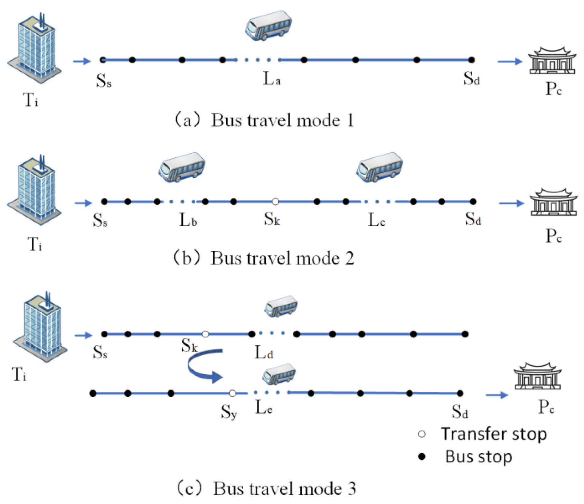
In the process of pilgrimage, for individual choosing public transportation to participate in pilgrimage activities, starting from the traffic zone , it is necessary to choose different public transportation lines when traveling to the pilgrimage area . This involves two travel schemes: direct and transfer. The direct travel scheme refers to the pilgrim , who starts from traffic zone , chooses the bus line , arrives at the bus stop , and then arrives at the pilgrimage area . This is shown in Figure 1a. Transfer travel schemes can be divided into two types: (I) Transfer at the same station refers to the pilgrimage individual , who starts from the traffic zone , selects the bus line , transfers at the bus stop , and takes the bus line to the pilgrimage area . This is shown in Figure 1b. (II) Transfer at different stations refers to the pilgrimage individual , who starts from the traffic zone , transfers at the bus stop of the bus line , and uses various modes such as walking, riding a bicycle, and driving a motor vehicle. Then, this pilgrim transfers to the bus line and then arrives at the pilgrimage area for pilgrimage activities. This is shown in Figure 1c.
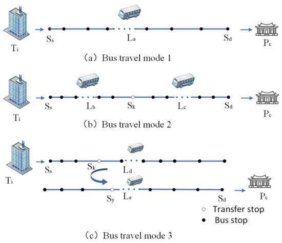
Figure 1.
The travel schemes of bus travel and transfer for pilgrimage. (a) Direct model; (b) Transfer at the same station; (c) Transfer at different stations.
During the pilgrimage, pilgrims experience the problem of changing transportation routes.
For different stop transfers, in this paper, only the network of the pedestrian transfer mode is constructed. In the process of constructing the transfer network and measuring the travel equity of pilgrimage travel, the following three standards were adopted:
- (1)
- For uplink and downlink lines, the bus line is abstracted as an undirected network according to the stop location and bus line of the actual line.
- (2)
- In the process of constructing the transfer network, the bus line between the starting bus stop and the ending bus stop shall be constructed with the shortest time as standard.
- (3)
- Because certain traffic districts are far away from bus stops (resulting in a lack of bus stops within the scope of the traffic district), when ArcGIS is used for accessibility measurement, the time for walking to the nearest bus stop is calculated. This reflects the time accessibility basis for the traffic district to choose bus travel.
Therefore, in this paper, the same-stop and different-stop transfer sub-networks are constructed first, both of which cooperate to realize the construction of the bus transfer network. Secondly, based on the network, the time accessibility of stops and the time accessibility of traffic zones are measured. Finally, spatial equity is measured based on the measurement results combined with global and local autocorrelation models. The specific steps are summarized in the following.
- Step 1: Constructing the transfer sub-network at the same stop.
Step 1.1: Connecting the stops on a single bus line according to the Space-P model, and then realizing the basic network construction of a single bus line.
Step 1.2: According to the actual bus routes in the study area, the OD cost matrix network analysis tool in ArcGIS is used. This is combined with the line operation time, transfer time, stop waiting time, and intersection waiting time of bus lines from the starting stop (i) to the destination stop (j) of the actual bus line route. Then, the overall operation time of each bus line is calculated. The specific calculation model is described in the following.
Measurement formula of bus line running time:
where refers to the line running time from stop to stop (unit: min), and represents the minimum time for stop to reach stop through the bus network. represents the transfer time, and represents the number of intersections at which stop can be reached from stop through the bus network. is the probability that the bus stops at a signalized intersection, i.e., the probability that the bus encounters a red light at a signalized intersection, expressed as . The average effective green light duration and the average period of the signalized intersection are and , respectively. represents the waiting time for passing through the intersection, represents the number of passing stops from stop to stop through the bus network, and represents the dwell time through the stop.
Step 1.3: Using the data export tool in ArcGIS to export and organize time-related data.
Step 1.4: Assigning values to the basic network connection lines of each bus line and then obtaining the same-stop transfer sub-network map.
- Step 2: Constructing the walking transfer sub-network.
Step 2.1: Based on the buffer tool in ArcGIS, bus stops within the walking transfer range of the target stop are extracted.
Step 2.2: According to the Space-P model, bus stops within the transfer range of the target stop are connected to each other; on this basis, the network construction of pedestrian transfer for a single bus stop is realized.
Step 2.3: According to the urban road routes in the study area, through the network analysis tool in ArcGIS, the target stop (c) is taken as a research source point, and the extracted bus stops within the transfer range are taken as destination points (d). Combined with the waiting time and walking time at the intersection of the actual road line, the walking transfer time of each bus stop is measured. The specific calculation model is presented in the following:
The formula for measuring the walking time is:
where, represents the walking running time from stop to stop (unit: ). represents the minimum walking time from stop to stop through the urban road network, and represents the number of crossings from stop to stop through the bus network. represents the waiting time for passing the intersection.
Step 2.4: Using the data export tool in ArcGIS, the data related to the walking transfer time between the lines at each stop are exported and processed, and values are assigned to the network connection lines of the lines at each stop.
Step 2.5: Based on the data link function of ArcGIS, after the extracted walking transfer time has been linked one by one according to the stop number, the basic network connection line of each bus stop is assigned. Then, the walking transfer sub-network diagram is obtained.
- Step 3: Constructing the bus travel network. Combined with the results of each transfer sub-network obtained in Steps 1 and 2, the two cooperate to realize the construction of the bus transfer network based on ArcGIS.
- Step 4: Stopping time accessibility. Combined with the bus transfer network constructed in Step 3, the average running time from each stop to the destination stop (research source point (C) is calculated based on the stop time accessibility measurement model (1). The pilgrimage time accessibility of each stop is measured by measuring the average running time of each stop.
Time accessibility measurement model:
In Equation (3), represents the accessibility of pilgrimage time at stop (unit: ). refers to the running time of the bus line passing through stop , and reaching stop through the bus network. represents the number of lines that stop passing through to stop through the bus network. represents the walking transfer time when stop arrives at stop through the walking transfer network. represents the number of walking and transfer times when stop reaches stop through the bus network.
- Step 5: Time accessibility of traffic zones. Using the pilgrimage time accessibility values of stops calculated in Step 4, the pilgrimage time accessibility of each traffic zone is calculated based on the time accessibility measurement model (2) of traffic zones.
Time accessibility model of traffic zones:
where represents the pilgrimage time accessibility of the bus in the traffic zone (unit: min). represents the pilgrimage time accessibility of bus stop in traffic zone , and represents the number of bus stops in traffic zone .
- Step 6: Spatial equity measurement
Step 6.1: Global spatial autocorrelation model. The global spatial autocorrelation model can be used to verify the correlation between attributes in a certain research area and the same attributes in adjacent research areas. The correlation relationship between the attributes of this research area includes positive correlation, negative correlation, and mutual independence. Moran’s I is the most commonly used method to calculate the global autocorrelation index, which is calculated as follows:
Global spatial autocorrelation model [36]:
In Equation (5), represents the variance value of public transport accessibility. represents the mean of accessibility of all traffic zones. and are the time accessibility of traffic zone and traffic zone , respectively, and represents the spatial distance weight between traffic zones. In this paper, the weight = 1 when there is a zone boundary between traffic zone and traffic zone , and = 0 when there is no zone boundary.
Step 6.2: Local spatial autocorrelation model. In the actual spatial data distribution, when the amount of data is too large, variable data often appear in the local area. The local instability of data is caused by its randomness. In that case, the local spatial autocorrelation index is introduced to realize the autocorrelation evaluation of the local area, and to obtain the spatial heterogeneity of the data.
Local spatial autocorrelation model [37]:
In Equation (6), is the total number of traffic zones. The sign of depends on and . reflects the level of accessibility between traffic zone i and Chengguan District as a whole, and reflects the level of accessibility between traffic zone around traffic zone and Chengguan District as a whole. Both formulas have high and low possibilities.
Step 6.3: Through the spatial cluster analysis method, combined with the meaning of global index and local index (see Table 1 and Table 2), the equilibrium results of public transport resource allocation can be divided into four categories. These are the high high allocation superior type, low low allocation backward type, high low allocation prominent type, and low high allocation trough type.

Table 1.
Range and meaning of Moran’s I index.
Table 2.
Value range and meaning of local Moran’s I index.
4. Details and Data of the Study Area
More than seven million Tibetans live in China, distributed throughout many provinces, including the Tibet Autonomous Region, Gansu Province, and Sichuan Province. Lhasa, the holy city of the Tibetan people, attracts many pilgrims from China and internationally. With changing times, pilgrimage in Lhasa has evolved into a social custom that has been integrated into the life of the Tibetan community. Therefore, this paper chose Lhasa as the case city for evaluating the travel space fairness of pilgrims. Of note, during national and religious festivals, many pilgrims arrive from outside, and local governmental departments set up special bus lines for this sudden increase in the bus passenger flow caused by pilgrims. This paper mainly focuses on the non-holiday travel of pilgrims. By measuring the spatial fairness of pilgrims in Lhasa, a new method for measuring the travel fairness of pilgrims in other regions can be obtained, thus providing a valuable case for the universality of the research results.
The data source for this paper is based on data obtained from the research on the life of pilgrims, pilgrimage areas, and bus routes in Lhasa during the period from March 2021 to June 2022. During the survey period, the number of new patients with COVID-19 in Lhasa was zero. Therefore, for the investigation data and public transport information used in this paper, there is no need to consider the impact of the COVID-19 pandemic. According to the bus lines in Lhasa, by the end of 2021, there are 38 bus lines in the Chengguan District of Lhasa. At the same time, Lhasa, as the holy city of Tibetan Buddhism, is a typical pilgrimage city. Therefore, Lhasa was selected to measure the time accessibility of public transport travel of pilgrims and both measure and analyze the spatial fairness of each traffic zone.
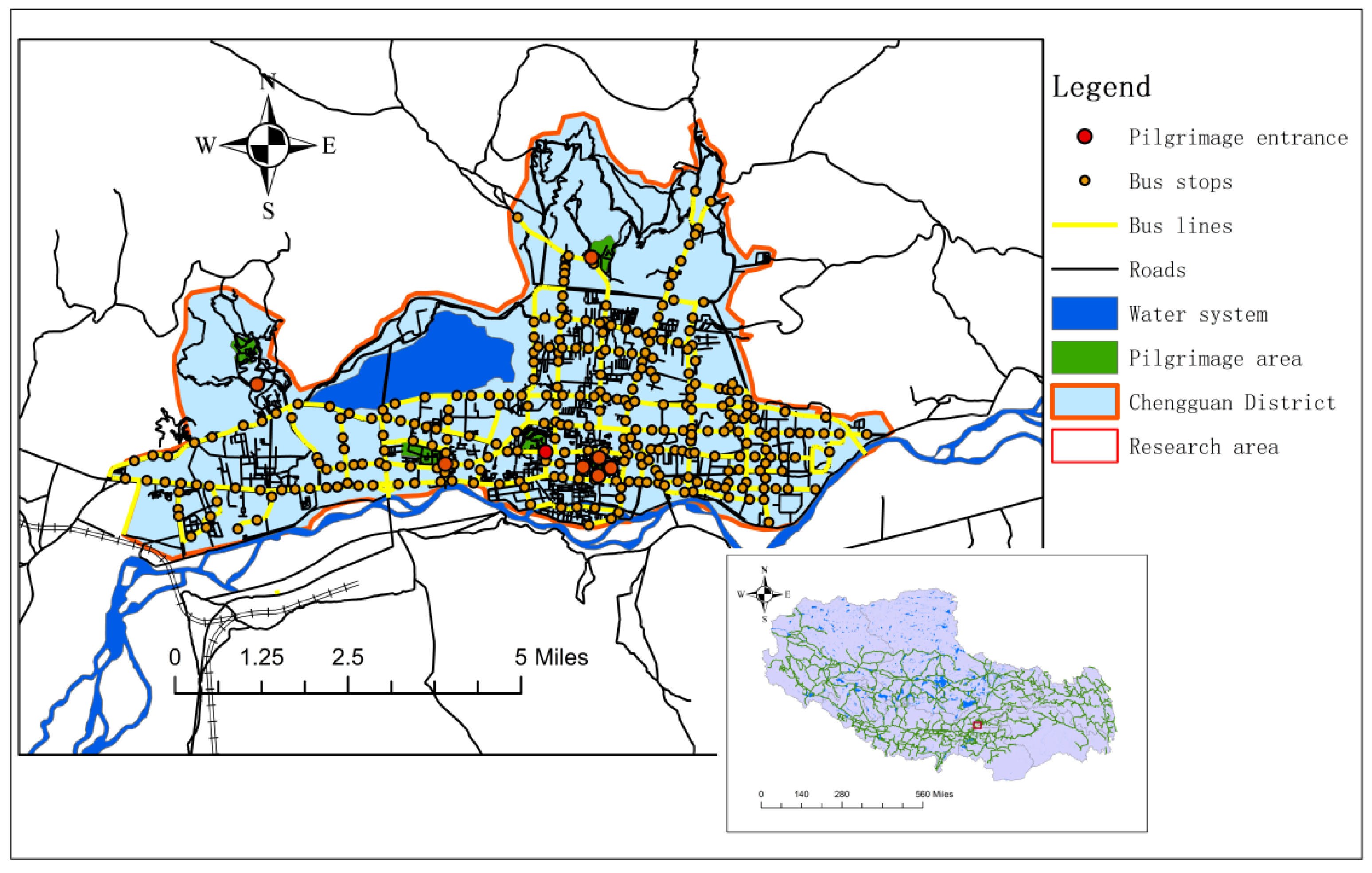
Combined with the regional administrative district planning map of Lhasa and a high-resolution remote sensing map, the geographical registration of the study area was carried out. ArcGIS was used to collect basic data on the pilgrimage public transportation network (i.e., basic information on bus routes, stops, and roads). The data were imported into the database constructed in ArcGIS in the form of a ShapeFile file by editing and importing. After summarizing and processing the data, a basic information database of pilgrimage bus travel routes in the Chengguan District of Lhasa was constructed, as shown in Figure 2.
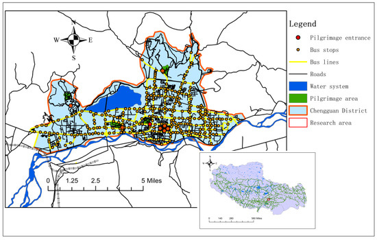
Figure 2.
Basic route data map of Lhasa.
Based on a Baidu map remote sensing image and administrative planning map, ArcGIS is used to draw the pilgrimage area. The Potala Palace District, Norbulingka Park, Jokhang Temple District, Drepung Monastery District, and Sera Monastery District (where five national festival pilgrimages are concentrated) were selected as research destinations. Combined with ArcGIS, the basic database information of the research object is compiled, including the name, area, address, and other information on the destination. Combined with the crowd aggregation of the research destination, the security checkpoint (or entrance and exit) of the destination is selected as a source point to obtain relevant data. Each research purpose includes multiple source points. For special instructions, for the Drepung temple area and the Sera temple area, the dividing point between internal roads and external roads is selected as the research source point. The research source points of five research destinations are drawn, as shown in Figure 2.
The public transport travel network is constructed according to the field investigation of public transport transfer problems in Lhasa, combined with basic information on public transport travel roads and the source information on pilgrimage research. In this paper, the walking transfer range is set to 500 m, and the public transportation network for pilgrimage is constructed.
During the division of the transportation community in the Chengguan District of Lhasa city, the overall planning of Lhasa city was fully considered. Combined with the regional economic development within the scope of the study, the division of the pilgrimage transportation community can coordinate the current situation of bus operation and the basic distribution of the pilgrimage population in the study area as much as possible. The study area is divided into 47 traffic districts, the specific distribution of which is shown in Figure 3.
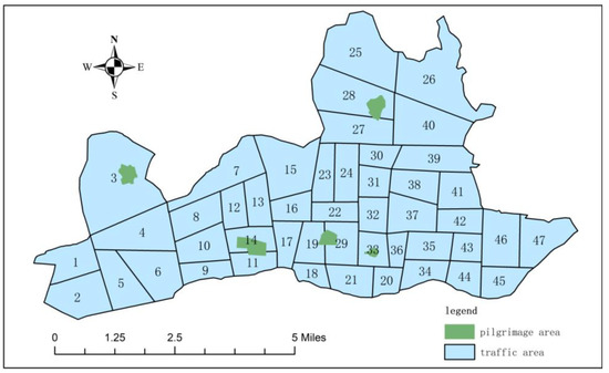
Figure 3.
Distribution map of traffic zones.
In this paper, the impact of different grades of roads on public transport travel in Lhasa is investigated. The survey results show that compared with mainland cities, Lhasa is an economically underdeveloped city, and the city scale is relatively small. Consequently, the road grade exerts little impact on the public transport travel of pilgrims. Therefore, the impact of the urban road grade on bus accessibility is not considered in the study, i.e., urban roads are not graded. At the same time, combined with the actual situation of public transport operation in Lhasa and field survey data, public transport operation parameters during national festivals involved in the public transport accessibility assessment are calibrated. The average speed of public transport is 30 km/h, the stop time at bus stops is 15 s, the average waiting time for signals at intersections is 30 s, and the average transfer time at stops is 5 min.
5. Results and Discussion
5.1. Time Accessibility Measure of Bus Stops
The ArcGIS network analysis method was used to measure and analyze the accessibility of bus stops serving pilgrimage travel. By sorting the accessibility values of the stops, the top 10 bus stops with the best accessibility within the research range as well as the 10 bus stops with the worst accessibility were obtained, as shown in Table 3.
Table 3.
Time accessibility of bus stops.
As shown in Table 3, the accessibility results of bus stops indicate that the Museum has the best accessibility at 3.24 min, followed by Norbulingka South at 3.40 min and La Bai at 3.62 min. Accessibility is worst for Duodi Township at 29.3 min, and the accessibility index is 9 times that of the Museum. The average accessibility of all bus stops is 15.89 min, and the accessibility value of Duodi Township is 29.3 min, which is 1.84 times the average of the accessibility indices of all stops. Statistics on the stops above the average value of the accessibility index show that there are 142 stops that exceed the average value for 15.89 min, accounting for 47.18% of the total number of stops. In contrast, stops that are lower than the average value of the accessibility index account for 52.82%, or a total of 159 bus stops.
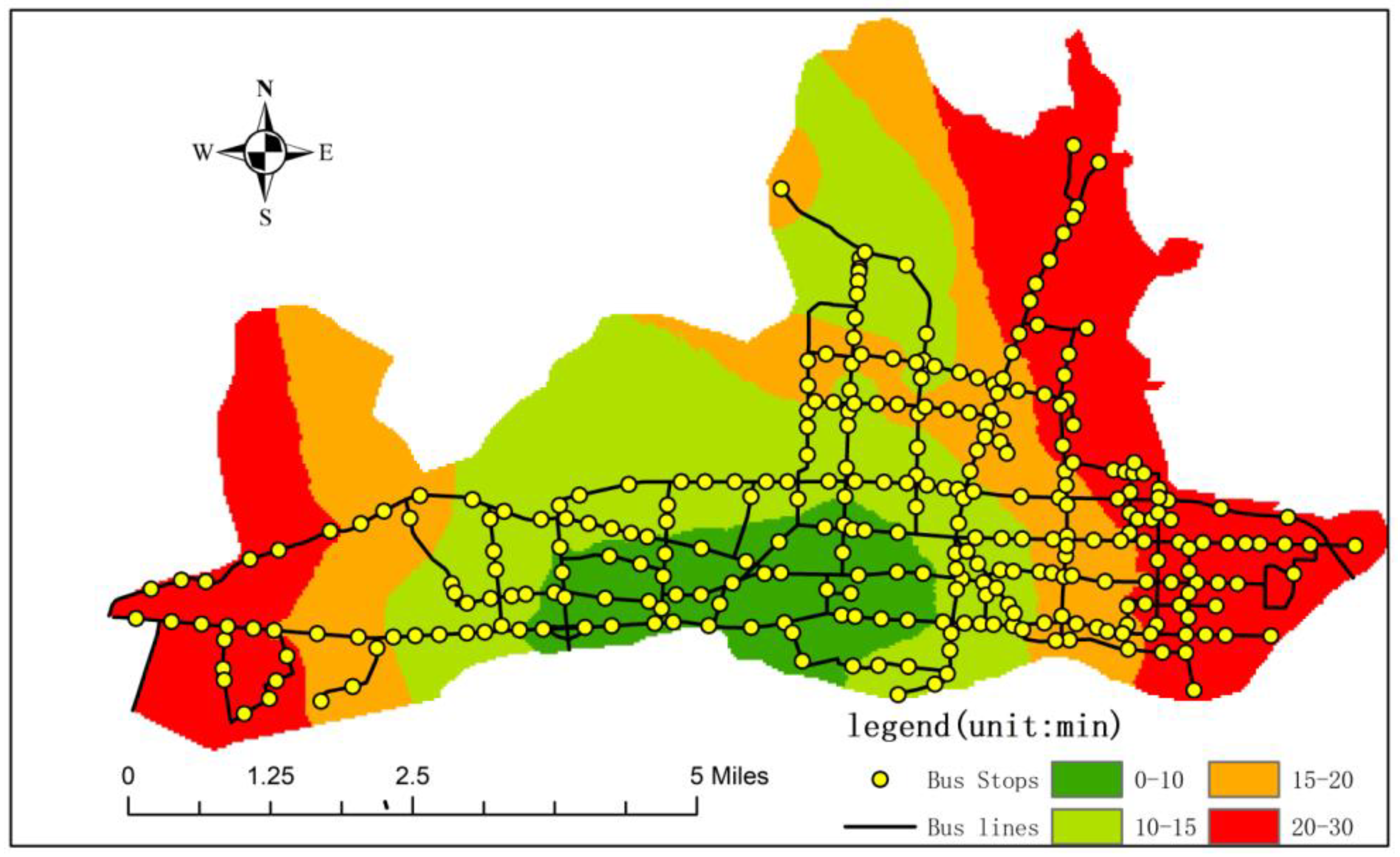
The time accessibility distribution map shown in Figure 4 reflects the convenience of public transportation for pilgrimage travel in Chengguan District. The colors in Figure 4 transition from green to red. The green areas indicate that the time resistance to be overcome from the area to the pilgrimage area is small, i.e., the accessibility is high, which also means that the time accessibility of the area is better. The red areas indicate the average time required for the area to reach the pilgrimage area. If this time is long, accessibility is poor, and it also means that the time accessibility of the area is poor. There are apparent differences in the accessibility of public transportation in space. Overall, the central area of the study area has the best time accessibility, and the time accessibility value is less than 10 min. The public transport accessibility in the study area presents a spatial distribution pattern that gradually decreases with increasing distance from the central area. Stops with poor temporal accessibility of bus stops are mainly distributed in the east and west of the study area. This result is similar to the research results of El-geneidy et al. [38], who used the number of jobs that can be obtained by marginalized groups within a specified travel time threshold as an indicator of accessibility for evaluating fairness.

Figure 4.
Time accessibility distribution map of pilgrimage stops.
5.2. Accessibility Measurement of Traffic Zones
Based on the measurement results of bus station time accessibility given and combined with the overall accessibility evaluation model of the pilgrimage traffic zones, the time accessibility of each traffic zone was calculated. The attribute table query function of ArcGIS software was used to calculate the time accessibility value of each traffic area, as shown in Table 4.
Table 4.
Time accessibility values of traffic zones.
After visualizing the time accessibility index of each traffic zone of Lhasa in ArcGIS, the classification display standard was calibrated. The index range was divided into traffic community accessibility grades of 0–10 min, 10–15 min, 15–20 min, and 25–40 min, corresponding to better, good, general, and poor traffic communities, respectively. The overall time accessibility distribution map of the Lhasa pilgrimage traffic community was drawn (as shown in Figure 5).
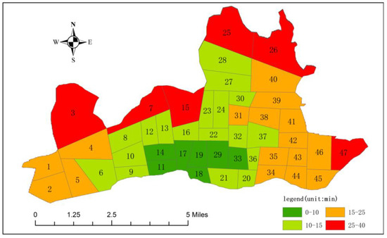
Figure 5.
Time accessibility distribution map of traffic zones.
The calculation results and spatial distribution of the accessibility of the traffic zone show that the accessibility of the pilgrimage traffic zone follows a spatial distribution pattern that spreads from the core area of the central city to the surrounding areas. This is related to the spatial distribution characteristics of the pilgrimage time accessibility of bus stops. Communities with better pilgrimage accessibility are mainly located in the central area of the study area. Among these areas, traffic zone 11 has the best pilgrimage time accessibility, with an accessibility value of 5.34 min. In the two directions of the northern and eastern areas of the central city of Lhasa, the traffic zone with the worst pilgrimage accessibility is traffic zone 25, with a pilgrimage accessibility value of 37.18 min. It is worth noting that in areas with good pilgrimage accessibility, there are also individual traffic zones with poor pilgrimage accessibility. For example, the time accessibility of traffic zone 15 is 28.31 min. This conclusion is similar to that of Chen et al. [39], who studied time accessibility from the perspective of green traffic, which evaluates traffic fairness through the accessibility of public transport and bicycles. Further in-depth investigation showed that the reason for the poor accessibility during pilgrimage time in this particular traffic zone is mainly that these areas are relatively remote and there are no bus lines in these areas (such as traffic zone 25), or if bus lines exist, there are no public transportation stops (such as traffic zone 3 and traffic zone 15). This leads to long walking distances and poor accessibility for traveling residents. The ArcGIS attribute table query function was used to obtain the time distribution frequency of the pilgrimage accessibility in the traffic zone (as shown in Table 5).
Table 5.
Time distribution frequency of time accessibility of traffic zones.
Analysis of the distribution law of the time accessibility of traffic zones showed that the average time accessibility of the traffic zones is 16.7 min. The time accessibility of 25 traffic zones is below the average, accounting for 53.19% of the total number of traffic zones in Lhasa. There are 22 traffic zones whose time accessibility is above the average time accessibility of all traffic zones, accounting for 46.81% of the total number of traffic zones. Seven areas have a time accessibility value of less than 10 min, accounting for about 15 of the total traffic zones, and their accessibility is good. Six traffic zones have an accessibility value of more than 25 min, accounting for 13% of the total number of traffic zones, and their accessibility is poor. The inequitable service of pilgrimage traffic in the traffic zone is even worse.
5.3. Equity of Space Allocation
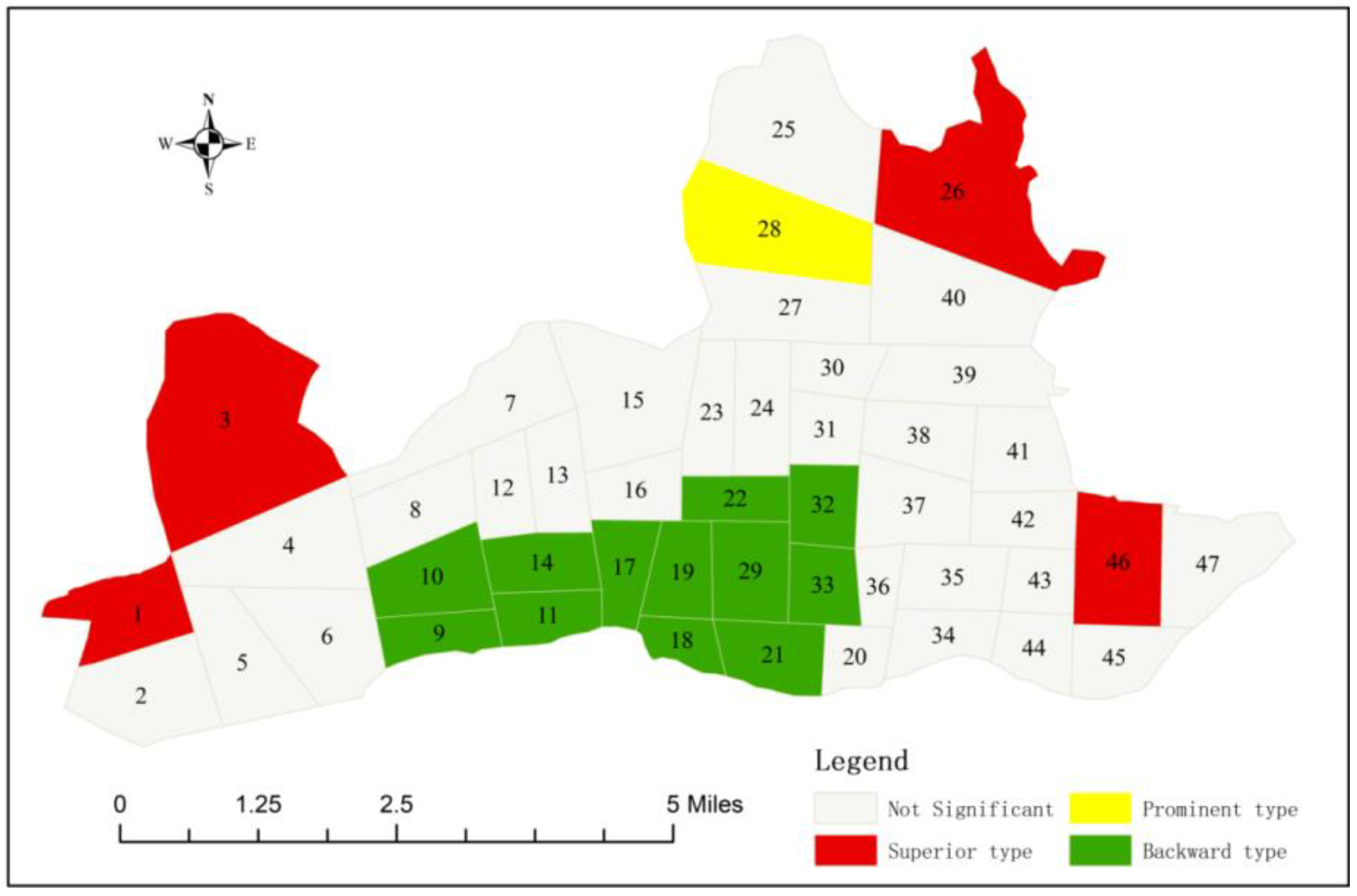
According to the accessibility data of traffic zones, the global clustering index of bus time accessibility of 47 traffic zones in Lhasa was calculated in the ArcGIS spatial statistical tool. The Moran’s I value is 0.487, the Z value is 5.615, and the p value is less than 0.01. The global clustering test results showed that the time accessibility of traffic zones in Chengguan District has a significant positive spatial correlation. Based on this, the local autocorrelation evaluation results are used to divide the resource allocation balance types of traffic zones in the study area into three types of areas: superior type, backward type, and prominent type (as shown in Figure 6).

Figure 6.
Resource allocation distribution of traffic zone.
5.3.1. Areas with Superior Allocation of Public Transport Resources
The local autocorrelation model indicates that the time accessibility of a certain traffic zone and its adjacent traffic zones is high. The global autocorrelation model indicates that the time accessibility of the traffic zone and its adjacent areas is positively correlated in space. As shown in Figure 6, these areas form the core areas of the urbanization development of Lhasa, which are quite good in terms of the allocation of roads and public transport infrastructure compared with non-core areas of Lhasa.
5.3.2. Areas with Backward Allocation of Public Transport Resources
The local autocorrelation model indicates that the time accessibility of the traffic zone itself is low, and the time accessibility of its adjacent traffic zones is also low. The global autocorrelation model indicates that the time accessibility of the traffic zone and its adjacent areas is positively correlated in space. As shown in Figure 6, the eastern and western border zones in the central urban area of Lhasa and traffic zone 26 in the north are traffic zones with backward allocation of public transport resources. These four traffic zones and surrounding traffic zones also have poor time accessibility.
5.3.3. Areas with Prominent Allocation of Public Transport Resources
The local autocorrelation model indicates that the time accessibility of the traffic zone itself is high, and the time accessibility of its adjacent traffic zones is low. The global autocorrelation model indicates that the time accessibility of the traffic zone and its adjacent zones is negatively correlated in space. As shown in Figure 6, only traffic zone 28 meets the conditions of such areas because the Sera temple is located in this area. Traffic zone 3 with Drepung temple is characterized by backward resource allocation. The reason is the low coverage of bus lines in the Drepung temple area compared with the Sera temple area. It can be concluded that the pilgrimage time accessibility of the stop is related to the location of the pilgrimage temple. However, the main reason is that the unreasonable line network planning and the unbalanced allocation of public transport resources are closely related. This shows that there is still an imbalance in the allocation of public transport resources in certain areas of the Chengguan District of Lhasa.
6. Conclusions
In this paper, the temporal accessibility and spatial autocorrelation model of bus lines are combined to study the spatial equity of pilgrimage travel. The aim is to better promote residential travel equity and achieve social equity. Several findings are summarized in the following:
Firstly, in this paper, ArcGIS is used to construct the pilgrim travel bus transfer network, which can be used to plan and analyze the bus travel route of pilgrims, and better reflect their travel behavior characteristics. This provides a new perspective for measuring the travel fairness of pilgrims in other regions of the world.
Secondly, both the stop accessibility measurement model and the traffic zone accessibility measurement model are used to measure the bus stop time accessibility and traffic zone time accessibility of pilgrimage, respectively. The reachability of the stop time can reflect the fairness and balance of the public transport system on pilgrimage travel well, and the traffic zoning can better reflect the rationality of the allocation of public transport resources of pilgrims in different regions. This provides a new measurement model for a better realization of travel equity and social equity from multiple perspectives. These results also provide a new perspective for studying the spatial fairness of different groups of people and can better reflect the fairness and balance of the traveling population.
Thirdly, the spatial fairness of pilgrimage travel is measured according to both the global spatial autocorrelation model and the local spatial autocorrelation model. Spatial autocorrelation analysis can reflect the spatial correlation of pilgrimage in the process of bus travel in various regions. It can also reflect the travel equity of pilgrimage travel in various regions, promote residential travel equity, and realize social equity.
In this paper, the travel equity of pilgrimage travel was studied from a spatial equity perspective. As an indispensable special group in the study of residential travel behavior, the in-depth study of this group is important for maximizing the use of the hard-won traffic resources of the Qinghai Tibet Plateau. This maximization can help to effectively meet the travel needs of pilgrims, form a pilgrimage travel organization and management system, provide high-quality travel services for pilgrims, and maintain normal travel order. In addition, public transport is not only the main mode of transportation for pilgrimage travel but also an important mode of transportation in the city. Public transport is a transportation service the which the whole of society has equal access. Fairness of the public transport system not only ensures travel equity of pilgrimage but also provides an important guarantee for the travel equity of all residents in society.
Author Contributions
Conceptualization, G.C. and L.G.; methodology, L.G.; software, L.G.; validation, G.C. and L.G.; investigation, L.G.; resources, G.C.; data curation, T.Z.; writing—original draft preparation, L.G.; writing—review and editing, L.G.; visualization, T.Z.; funding acquisition, G.C. All authors have read and agreed to the published version of the manuscript.
Funding
This research was supported by the National Natural Science Foundation of China (Grant No. 51968063), Himalayan human activities and regional development collaborative innovation construction center project (No. 00060872), Academic development support program for young doctors of Tibet University (No. zdbs202212) and Cultivation Project of Tibet University (Grant No. ZDTSJH19-01).
Institutional Review Board Statement
Not applicable.
Informed Consent Statement
Not applicable.
Data Availability Statement
Data are contained within the article. Any elaborations are available, upon request, from the authors.
Acknowledgments
The authors are very grateful to The Bus Company of the Lhasa Public Traffic Group, as well as investigators and respondents, who helped with our data collection.
Conflicts of Interest
The authors declare no conflict of interest.
References
- Foth, N.; Manaugh, K.; El-Geneidy, A.M. Towards equitable transit: Examining transit accessibility and social need in Toronto, Canada, 1996–2006. J. Transp. Geogr. 2013, 29, 1–10. [Google Scholar] [CrossRef]
- Karner, A. Assessing public transit service equity using route-level accessibility measures and public data. J. Transp. Geogr. 2018, 67, 24–32. [Google Scholar] [CrossRef]
- Patterson, Z.; Farber, S. Potential Path Areas and Activity Spaces in Application: A Review. Transp. Rev. 2015, 35, 679–700. [Google Scholar] [CrossRef]
- Wang, Y.; Chen, B.Y.; Yuan, H.; Wang, D.; Lam, W.H.K.; Li, Q. Measuring temporal variation of location-based accessibility using space-time utility perspective. J. Transp. Geogr. 2018, 73, 13–24. [Google Scholar] [CrossRef]
- Chen, B.Y.; Wang, Y.; Wang, D.; Li, Q.; Lam, W.H.K.; Shaw, S.-L. Understanding the impacts of human mobility on accessibility using massive mobile phone tracking data. Ann. Am. Assoc. Geogr. 2018, 108, 1115–1133. [Google Scholar] [CrossRef]
- Weiss, D.J.; Nelson, A.; Gibson, H.S.; Temperley, W.; Peedell, S.; Lieber, A.; Hancher, M.; Poyart, E.; Belchior, S.; Fullman, N.; et al. A global map of travel time to cities to assess inequalities in accessibility in 2015. Nature 2018, 553, 333–336. [Google Scholar] [CrossRef]
- Zhang, T.; Dong, S.; Zeng, Z.; Li, J. Quantifying multi-modal public transit accessibility for large metropolitan areas: A time-dependent reliability modeling approach. Int. J. Geogr. Inf. Sci. 2018, 32, 1649–1676. [Google Scholar] [CrossRef]
- Conway, M.W.; Byrd, A.; Van Eggermond, M.A. Accounting for uncertainty and variation in accessibility metrics for public transport sketch planning. J. Transp. Land Use 2018, 11, 541–558. [Google Scholar] [CrossRef]
- Martens, K. Justice in transport as justice in accessibility: Applying Walzer’s ‘Spheres of Justice’ to the transport sector. Transportation 2012, 39, 1035–1053. [Google Scholar] [CrossRef] [Green Version]
- Lucas, K. Transport and social exclusion: Where are we now? Transp. Policy 2012, 20, 105–113. [Google Scholar] [CrossRef]
- Tao, S.; He, S.Y.; Kwan, M.-P.; Luo, S. Does low income translate into lower mobility? An investigation of activity space in Hong Kong between 2002 and 2011. J. Transp. Geogr. 2020, 82, 102583. [Google Scholar] [CrossRef]
- Wang, H.; Kwan, M.-P.; Hu, M. Social exclusion and accessibility among low- and non-low-income groups: A case study of Nanjing, China. Cities 2020, 101, 102684. [Google Scholar] [CrossRef]
- Moniruzzaman, M.; Chudyk, A.; P’aez, A.; Winters, M.; Sims-Gould, J.; McKay, H. Travel behavior of low income older adults and implementation of an accessibility calculator. J. Transp. Health 2015, 2, 257–268. [Google Scholar] [CrossRef] [PubMed]
- Hahn, J.-S.; Kim, H.-C.; Kim, J.-K.; Ulfarsson, G.F. Trip making of older adults in Seoul: Differences in effects of personal and household characteristics by age group and trip purpose. J. Transp. Geogr. 2016, 57, 55–62. [Google Scholar] [CrossRef]
- Feng, J. The influence of built environment on travel behavior of the elderly in urban China. Transp. Res. Part D Transp. Environ. 2017, 52, 619–633. [Google Scholar] [CrossRef]
- Allen, J. Mapping differences in access to public libraries by travel mode and time of day. Libr. Inf. Sci. Res. 2019, 41, 11–18. [Google Scholar] [CrossRef]
- Hu, L.; Fan, Y.; Sun, T. Spatial or socioeconomic inequality? Job accessibility changes for low- and high-education population in Beijing, China. Cities 2017, 66, 23–33. [Google Scholar] [CrossRef]
- Shao, F.; Sui, Y.; Yu, X.; Sun, R. Spatio-temporal travel patterns of elderly people—A comparative study based on buses usage in Qingdao, China. J. Transp. Geogr. 2019, 76, 178–190. [Google Scholar] [CrossRef]
- Cheng, G.; Jiang, S.; Zhang, T. Fuzzy Multidimensional Assessment Approach of Travel Deprivation in Small Underdeveloped Cities: Case Study of Lhasa, China. J. Adv. Transp. 2021, 2021, 8851449. [Google Scholar] [CrossRef]
- Cheng, G.; Zhao, S.; Huang, D. Understanding the Effects of Improving Transportation on Pilgrim Travel Behavior: Evidence from the Lhasa, Tibet, China. Sustainability 2018, 10, 3528. [Google Scholar] [CrossRef] [Green Version]
- Mayaud, J.R.; Tran, M.; Nuttall, R. An urban data framework for assessing equity in cities: Comparing accessibility to healthcare facilities in Cascadia. Comput. Environ. Urban Syst. 2019, 78, 101401. [Google Scholar] [CrossRef]
- Stanley, B.W.; Dennehy, T.J.; Smith, M.E.; Stark, B.L.; York, A.M.; Cowgill, G.L.; Novic, J.; Ek, J. Service access in premodern cities: An exploratory comparison of spatial equity. J. Urban Hist. 2016, 42, 121–144. [Google Scholar] [CrossRef] [Green Version]
- Lievrouw, L.A.; Farb, S.E. Information and equity. Annu. Rev. Inf. Sci. Technol. 2003, 37, 499–540. [Google Scholar] [CrossRef]
- Dadashpoor, H.; Rostami, F. Measuring spatial proportionality between service availability, accessibility, and mobility: Em-pirical evidence using spatial equity approach in Iran. J. Transp. Geogr. 2017, 65, 44–55. [Google Scholar] [CrossRef]
- Arranz-López, A.; Soria-Lara, J.A.; Pueyo-Campos, Á. Social and spatial equity effects of non-motorised accessibility to retail. Cities 2019, 86, 71–82. [Google Scholar] [CrossRef] [Green Version]
- Cheng, W.; Wu, J.; Moen, W.; Hong, L. Assessing the spatial accessibility and spatial equity of public libraries’ physical locations. Libr. Inf. Sci. Res. 2021, 43, 101089. [Google Scholar] [CrossRef]
- Sin, S.-C.J. Neighborhood disparities in access to information resources: Measuring and mapping U.S. public libraries’ funding and service landscapes. Libr. Inf. Sci. Res. 2011, 33, 41–53. [Google Scholar] [CrossRef]
- Witten, K.; Pearce, J.; Day, P. Neighbourhood Destination Accessibility Index: A GIS Tool for Measuring Infrastructure Support for Neighbourhood Physical Activity. Environ. Plan. A Econ. Space 2011, 43, 205–223. [Google Scholar] [CrossRef]
- Pritchard, J.P.; Tomasiello, D.B.; Giannotti, M.; Geurs, K. Potential impacts of bike-and-ride on job accessibility and spatial equity in São Paulo, Brazil. Transp. Res. Part A Policy Pract. 2019, 121, 386–400. [Google Scholar] [CrossRef]
- Park, S.J. Measuring public library accessibility: A case study using GIS. Libr. Inf. Sci. Res. 2012, 34, 13–21. [Google Scholar] [CrossRef]
- Brook, O. Spatial equity and cultural participation: How access influences attendance at museums and galleries in London. Cult. Trends 2016, 25, 21–34. [Google Scholar] [CrossRef] [Green Version]
- Kaplan, S.; Popoks, D.; Prato, C.G.; Ceder, A.A. Using connectivity formeasuring equity in transit provision. J. Transp. Geogr. 2014, 37, 82–92. [Google Scholar] [CrossRef]
- Tsou, K.-W.; Hung, Y.-T.; Chang, Y.-L. An accessibility-based integrated measure of relative spatial equity in urban public facilities. Cities 2005, 22, 424–435. [Google Scholar] [CrossRef]
- Donnelly, F.P. Regional variations in average distance to public libraries in the United States. Libr. Inf. Sci. Res. 2015, 37, 280–289. [Google Scholar] [CrossRef]
- Guo, Y.; Chan, C.H.; Yip, P.S. Spatial variation in accessibility of libraries in Hong Kong. Libr. Inf. Sci. Res. 2017, 39, 319–329. [Google Scholar] [CrossRef]
- Moran, P.A.P. Notes on continuous stochastic phenomena. Biometrika 1950, 37, 17–23. [Google Scholar] [CrossRef]
- Anselin, L. Local Indicators of Spatial Association—LISA. Geogr. Anal. 1995, 27, 93–115. [Google Scholar] [CrossRef]
- El-Geneidy, A.; Levinson, D.; Diab, E.; Boisjoly, G.; Verbich, D.; Loong, C. The Cost of Equity: Assessing Transit Accessibility and Social Disparity Using Total Travel Cost. Transp. Res. Part A Policy Pract. 2016, 91, 302–316. [Google Scholar] [CrossRef] [Green Version]
- Chen, N.; Wang, C.-H. Does green transportation promote accessibility for equity in medium-size U.S. cites? Transp. Res. Part D Transp. Environ. 2020, 84, 102365. [Google Scholar] [CrossRef]


Publisher’s Note: MDPI stays neutral with regard to jurisdictional claims in published maps and institutional affiliations. |
© 2022 by the authors. Licensee MDPI, Basel, Switzerland. This article is an open access article distributed under the terms and conditions of the Creative Commons Attribution (CC BY) license (https://creativecommons.org/licenses/by/4.0/).