Article

Analytical Solution of the Mixed Traffic Flow Cellular Automaton FI Model with the Next-Nearest-Neighbor Interaction

1
Institute of Physical Science and Technology, Guangxi University, Nanning 530004, China
2
Guangxi Key Lab Relativist Astrophys, Nanning 530004, China
*
Author to whom correspondence should be addressed.
Sustainability 2022, 14(12), 7127; https://doi.org/10.3390/su14127127
Submission received: 1 May 2022 / Revised: 1 June 2022 / Accepted: 6 June 2022 / Published: 10 June 2022

Abstract

:
Based on a one-dimensional (1D) traffic flow cellular automaton (CA) FI model, a deterministic next-nearest-neighbor interaction FI model (NIFI model) is proposed. Using the mean-field analysis, the analytical solution of the NIFI model in one-dimensional traffic flow is derived under periodic boundary conditions. For the mixed traffic flow, the occupancy and the mixing ratio are introduced to describe the mixing effect. Similarly, using the mean-field method, the exact solution of the mixed traffic flow is derived from the long-time evolution to reach the steady state. The numerical simulations are carried out for the mixed traffic flow with different vehicle lengths, maximum velocities, and mixing ratios to verify the analytical solutions. The results show that the numerical simulation results agree well with the analytical solution.

1. Introduction

In recent years, traffic congestion and traffic accidents are becoming increasingly serious. Research on traffic flow issues helps people to better predict road traffic conditions. Recently, there have been various traffic flow models to study the traffic flow problems, such as the cellular automata model, the car-following model, and so on [1]. Among these models, the CA (cellular automata) model has been conveniently implemented on computers due to its simple evolution rules and computational efficiency. Moreover, the CA model can be flexibly adjusted to the applications according to the actual situation, so it has good practical significance [1,2,3,4]. The CA model can not only simulate the traffic flow of single lane [3,5], complex three-phase traffic flow [6], and urban road networks [4], but also study traffic fuel consumption [7], pollutant emission [8,9,10], and traffic control [11,12], etc.
The cellular automata describing the most primitive form of highway traffic flow is a cellular automata named CA model, Rule 184 [2]. Based on the 184 model, Nagel and Schreckenberg have proposed the NaSch cellular automaton traffic flow model, which reflects the features of gradual acceleration, deceleration, and randomization in realistic traffic flows [3]. To simulate a variety of phenomena in actual traffic measurements, various improvement models have been developed [5,6,13]. In 1996, Fukui and Ishibashi proposed the CA FI model to improve the acceleration process of a vehicle. The FI model can simulate the acceleration behavior of a vehicle at an intersection to a certain extent [5]. Wang et al. studied the FI model numerically and analytically and obtained the average velocity <V(t→∞)> in the long-time limit as a function of car density, called the fundamental diagram [14]. Wang L et al. strictly derived the mean-field equation for a one-dimensional CA FI model [15,16]. The solution <V(t→∞)> in the NaSch model without random delay was obtained by tracing the time evolution of car spacing [17]. In 2007, Fu et al. proposed the modified Nagel–Schreckenberg model with the Fukui–Ishibashi acceleration rule and gave the corresponding analytical solution [18]. Jia and Ma carried out an analytical investigation of the open boundary conditions in the Nagel–Schreckenberg model. They found an effective approach for deducing the analytical expression of inflow [19]. Jia and Ma studied the deterministic Nagel–Schreckenberg model with stochastic open boundary conditions in an analytical way. The analytical expression of the free-flow density profiles was derived [20]. Ding et al. investigated the Biham–Middleton–Levine model with a random update rule and found the coexistence of the moving phase and jamming phase under open boundary conditions. They presented a mean-field analysis of the moving phase [21]. In more recent years, Ding et al. proceeded the mean-field analysis of asymmetric exclusion processes on two parallel lattices with fully parallel dynamics and derived an analytic solution [22]. In 1999, Nagatani first proposed an optimal velocity model considering the next-nearest-neighbor interaction [23]. The researcher discovered that the next-nearest-neighbor interaction stabilizes the traffic flow, and the jamming transition between the freely moving and jamming phases occurs at a higher density than the threshold of the original optimal velocity model. Li et al. presented a CA model called the Velocity Effect (VE) model by considering the influence of the distance between the nearest neighbor and the next nearest neighbor on the current vehicle motion. The simulation displays that there exists a metastable state and hysteresis phenomenon under deterministic conditions [24]. Ge et al. proposed an extended car-following model to study the influence of multiple vehicles ahead on traffic flow. Their research shows that anticipating the behavior of more vehicles ahead leads to the stabilization of traffic systems [25]. However, the CA FI model taking the next-nearest-neighbor interaction into account has not been studied. Therefore, we proposed a deterministic next-nearest-neighbor interaction FI model (NIFI model for short) for single and mixed traffic flow. The mixed traffic flow consists of different vehicle lengths and the maximum velocity. By using the mean-field theory, we will attempt to derive the mean-field solutions of the deterministic NIFI model of single traffic flow and mixed traffic flow, respectively.
The arrangement of this paper is organized as follows: By incorporating the evolution rule of vehicles in Section 2, we present a deterministic next-nearest-neighbor interaction FI model (NIFI model). The analytical solution of the NIFI model in one-dimensional single traffic flow and mixed traffic flow is derived by using CA mean-field theory. In Section 3, the analytical solution of the NIFI model is verified by numerical simulation. Some conclusions are drawn in Section 4.

2. Methodology

2.1. NIFI Model

The Nagel–Schreckenberg (NaSch) model and the Fukui–Ishibashi (FI) model are two typical one-dimensional cellular automata traffic flow models. In the deterministic FI model, the evolution of each vehicle’s velocity is carried out according to the following parallel updating rules.
V i ( t + 1 ) min ( V max , gap i )
where V max denotes the maximum velocity, and gap i is the headway between the (i + 1)th vehicle and the ith one.
gap i = X i + 1 ( t ) X i ( t ) l
V i ( t ) and X i ( t ) , respectively, denote the velocity and position of the ith vehicle on the road at time step t, and l denotes the vehicle length. If the traffic flow consists of the same vehicle, the vehicle length is taken as the unit length to occupy a cell (l = 1).
Taking the next-nearest-neighbor interaction into account, the following update rule of the deterministic NIFI model can be obtained by embedding the deterministic FI model velocity update rule. The positions and velocities of all vehicles are updated at the same time.
Step 1. Determine the velocity of the next time step:
V i ( t + 1 ) min ( V i max , ( gap i + min ( V i + 1 max , gap i + 1 ) ) )
Step 2. Move forward.
X i ( t + 1 ) X i ( t ) + V i ( t + 1 )
where V i + 1 max and V i max are the maximum velocity of the (i + 1)th vehicle and the ith vehicle, respectively. Under periodic boundary conditions, the road is a closed-loop chain composed of L cells. The vehicles in a single traffic flow consisting of the same vehicles have the same length and occupy a cell in the simulation process.
For a mixed traffic flow composed of long and short vehicles, each cell may be occupied by a vehicle with a disparate length or no vehicle at all. The vehicle velocity of the occupied cell ranges from 0 to a maximum velocity, Vmax. The short vehicle and the long vehicle take up lS cells and lL (lL > lS) cells, respectively. At each evolutionary time step, all vehicle states are updated in parallel according to evolution rules (3) and (4).
To describe the mixed traffic flow, the occupancy rate is introduced. The occupancy C is defined as follows:
C = N L l L + N S l S L
where the number of the long vehicle and the short vehicle, respectively, is denoted as N L and N s . The maximum velocity of the long and short vehicles is, respectively, expressed as V L max and V S max . The mixing ratio C n is defined as C n = N S N , which is to measure the degree of mixing between the long and short vehicles. The global density is represented as ρ = N L , L is the length of road, and the total number of vehicles is equal to N = N L + N S . The global density is obtained as follows:
ρ = C C n l s + ( 1 C n ) l L

2.2. Analytical Solution of NIFI Model

At first, the traffic flow composed of the same type of vehicle was studied. Based on the mean-field method, we tried to derive the exact solution of the NIFI model in one-dimensional traffic flow under periodic boundary conditions. With the increasing number of vehicles on the road, the dynamic behavior of traffic flow will change. For low vehicle density ( ρ ρ c ), all vehicles on the road can move at their own maximum velocity V i max . For high vehicle density ( ρ > ρ c ), the vehicle cannot move with the maximum velocity in the next time step due to the distance between two consecutive vehicles being less than the maximum velocity, as well as the influence of the next-nearest-neighbor interaction. On average, when the evolution time is long enough ( t ), according to the velocity update rules of the NIFI model, the velocity of vehicles can be limited to the average gap. The average gap for the whole traffic flow can be calculated by dividing the total number of empty cells on the road that are not occupied by vehicles by the total number of vehicles. Therefore, the average gap can be represented by
gap ¯ = L i = 1 N l i N
where li is the length of the ith vehicle. When the vehicle density approaches the critical density ρ c , traffic flow changes from free flow to congestion. Under the condition of high vehicle density, the evolutionary step (3) of the NIFI model manifests that the motion of the ith vehicle must be accompanied by the motion of the (i + 1)th vehicle and the (i + 2)th vehicle in front considering the effect of the next-nearest-neighbor (i + 2)th vehicle in front, To put it another way, under the condition of high vehicle density, the ith vehicle can move forward at an average velocity of twice the average gap due to the movement of the next nearest neighbor. The average velocity V satisfies the following equation:
V = 2 × gap ¯ .
Thus, the average velocity is obtained from Equations (7) and (8):
V = 2 ( L i = 1 N l i N )   for   ρ > ρ c .
For one-dimensional single traffic flow, firstly, we discuss the situation where there is only one type of vehicle on the road. It is assumed that the length of the vehicle is 1 cell (li = 1). According to Equation (9), the following average velocity is acquired:
V = 2 ( 1 ρ 1 )   for   ρ > ρ c .
Since the average velocity at the critical density point ρ c is Vmax, there is the following equation:
V max = 2 ( 1 ρ c 1 )   ,
Therefore, the critical density is fielded:
ρ c = 2 V max + 2 .
Taking Equations (10) and (11) and velocity Vmax in free flow into consideration, the relation of the average velocity with vehicle density is obtained:
V = {   V max     0 ρ ρ c = 2 V max + 2   2 ( 1 ρ ) ρ     ρ c < ρ 1
For the deterministic FI model, the average velocity is expressed as follows [15,16]:
V = {   V max     0 ρ 1 V max + 1   1 ρ 1     1 V max + 1 < ρ 1
The analytical solution Equation (13) of the NIFI model is obviously different from Equation (14) of the deterministic FI model. The jamming transition between the freely moving and jamming phases occurs at a higher density than the threshold of the original deterministic FI model when the next-nearest-neighbor interaction is considered. Traffic flux J is defined as J = ρV, and the fundamental diagram of NIFI model is obtained as follows:
  J = { ρ V max       0 ρ ρ c = 2 V max + 2   2 ( 1 ρ )     ρ c < ρ 1
Next, we will study the mixed traffic flows with more than one type of vehicle on the road. For mixed traffic flow, different types of vehicles possess different vehicle lengths and maximum velocities. To describe the road occupied by vehicles more precisely, the density ρ , of vehicles on the road is replaced by the total occupancy C . Similarly, we can determine the relationship of the average gap and the average velocity V , with the occupancy C . Therefore, it can be concluded as follows from Equations (7) and (8):
gap ¯ = L ( 1 C ) N .
V = 2 L ( 1 C ) N
In mixed traffic flow, the maximum velocity of the long vehicle is V L max , and the maximum velocity of the short vehicle is V S max . As the evolution time is long enough (t→∞) to reach the steady state, vehicles with the higher maximum velocity cannot travel at their maximum velocity due to the obstruction effect of vehicles with smaller maximum velocity, even if the vehicle density is very small. Chowdhury et al. and Knospe et al. have discussed this blocking effect of slow vehicles when they studied lane changing using a cellular automata model, respectively [26,27]. As the evolution time is long enough (t→∞) for the mixed traffic flow to reach the steady state, vehicles with a large maximum velocity in the mixed traffic flow can only travel at a small maximum velocity. The maximum velocity in the mixed traffic flow is taken as a smaller maximum velocity.
V max = min ( V S max , V L max )
Similarly, at the critical occupancy, Cc, all vehicles can also travel at the maximum velocity V max . By substituting Equation (17) into Equation (18) and considering Equation (6), we can, thus, derive the following equation:
V max = 2 ( 1 C c ) ( C n l S + ( 1 C n ) l L ) C c .
The critical occupancy, Cc, of mixed traffic flow is obtained as follows:
C c = 2 V max ( C n l S + ( 1 C n ) l L ) + 2   or   ρ c = 1 V max 2 + ( C n l S + ( 1 C n ) l L ) .
Compared with the critical density of Equation (12), the critical occupancy, Cc, of mixed traffic flow also has a similar mathematical expression. When the length of a long vehicle is much higher than that of a short one, (lL > ls), Equation (20) can be simplified to the following equation:
C c 2 V max ( 1 C n ) l L ( 1 C n ( 1 C n ) l s l L ) + 2 2 V max ( 1 C n ) l L + 2
The critical occupancy, C c , is determined by the length of the long vehicle and the mixing ratio. When the number of long vehicles is equal to the number of short vehicles ( N L = N S , C n = 0.5), Equation (20) can be rewritten as follows:
C c = 1 V max l s + l L + 1
In this case, the length of the long vehicle and the short one together determines the critical occupancy, C c . As may be observed, C c , the critical density of mixed traffic flow, is higher than that of the single NIFI model by comparing Equation (20) with Equation (12), because the maximum velocity is reduced.
As time evolves to the steady state, vehicles can move with the maximum velocity at low occupancy. According to Equation (18), the average velocity of the free flow of the vehicle is V max . At high occupancy, the average velocity of the traffic flow is V rather than the maximum velocity V max . From Equations (6) and (17), the average velocity, V , of vehicles at high density is derived. Therefore, the average velocity vs. occupancy, C , is represented as the following relationship:
  V = { V max 0 C C c 2 ( 1 C ) [ C n l S + ( 1 C n ) l L ] C C c < C 1
The exact solution of the NIFI model of mixed traffic flow is quite different from that of the deterministic FI model from Equation (14) [15,16]. The corresponding equation of the fundamental diagram is:
  J = { C V max C n l S + ( 1 C n ) l L 0 C C c 2 ( 1 C ) C c < C 1
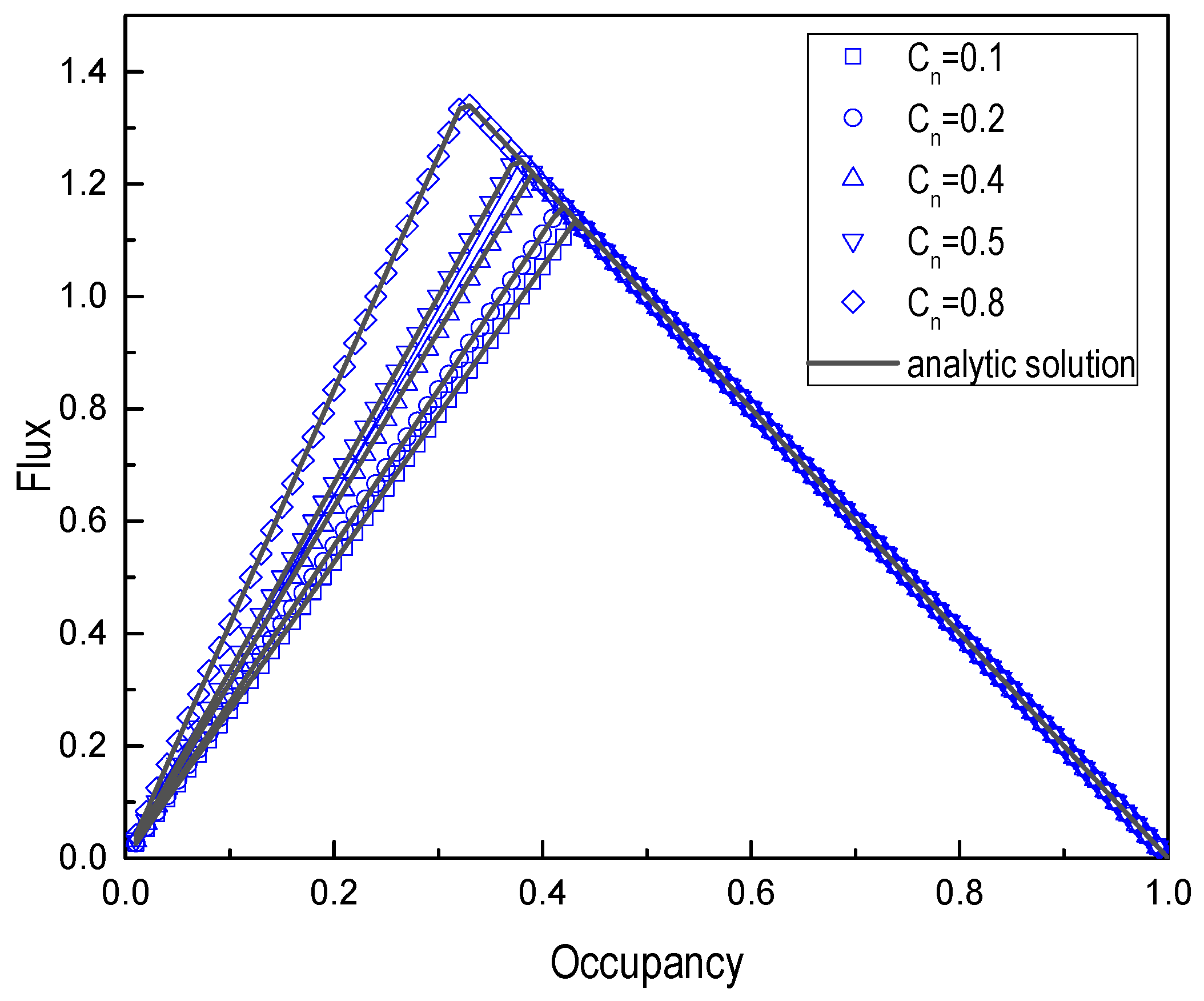
According to Equation (24), we can perform simulation experiments to obtain the fundamental diagram, which can reflect the movement of traffic flow on the road. At low density, the traffic flow is in the free-flow state of maximum velocity, while at high density, the traffic congestion is at low velocity. Based on Equation (24), we can figure out that the slope of curves from the equation of the fundamental diagram is:
  d J d C = { V max C n l S + ( 1 C n ) l L 0 C C c 2 C c < C 1
Equation (25) indicates that when the occupancy is small, the slope of a flow is related to the mixing ratio C n , and the mixture lengths of vehicles. In traffic congestion, the flow slope is not relevant to the mixture ratio C n . These conclusions will be confirmed in the following section of the numerical simulation.
When C n = 1, it is a special case of one-dimensional single traffic flow, and all vehicles are short ones (lS = 1), C = ρ , C c = 2 V max + 2 . The corresponding equation of the fundamental diagram is:
  J = { ρ V max 0 ρ 2 V max + 2 2 ( 1 ρ ) 2 V max + 2 < ρ 1
This result is consistent with Equation (15). When Cc = 0, it corresponds to a one-dimensional (1D) single traffic flow composed of long vehicles with the maximum velocity, V L max , C = ρ l L , C c = 2 l L V L max + 2 l L . The corresponding equation of the fundamental diagram is:
  J = { ρ V L max 0 ρ l L 2 l L V L max + 2 l L   2 ( 1 ρ l L ) 2 l L V L max + 2 l L < ρ l L 1
Clearly, it is different from Equation (26). If the size of a cell is the length of long vehicles (i.e., lL = 1), Equation (27) is in agreement with Equation (26).

3. Simulation

The fundamental diagram of the NIFI model is derived analytically to give the traffic flux as a function of vehicle density or occupancy. We perform a numerical simulation to verify its accuracy. For the computer simulation, the average velocity V of traffic flow is defined as follows:
V = 1 T 1 N t = t 0 + 1 t 0 + T i = 1 N v i ( t )
where t 0 is the relaxation time to reach the steady state. Traffic flux, J , is defined as J = ρ V .
We carried out numerical simulations on a one-dimensional chain consisting of L = 104 cells under periodic boundary conditions. All vehicles were randomly distributed along the lattice chain with a random velocity at the beginning. The simulation was performed with 50 independent runs in different initial configurations. Each run for 3 × 10⁴ iterations and the first 2 × 10⁴ iterations were discarded in measuring the quantities of interest.

3.1. Numerical Simulation for 1D Single Traffic Flow

Figure 1 and Figure 2, respectively, show the numerical simulation results and the analytical solutions of the average velocity and the traffic flux, J, for different maximum velocities. It shows that the result of numerical simulation is consistent with the analytical solution. The fundamental diagram for different maximum velocities shows the change of traffic flow from the free flow to the congested state with the increase of the density.

3.2. Numerical Simulation of the Mixed Traffic Flow

3.2.1. Effect of Mixing Ratio on Mixed Traffic Flow

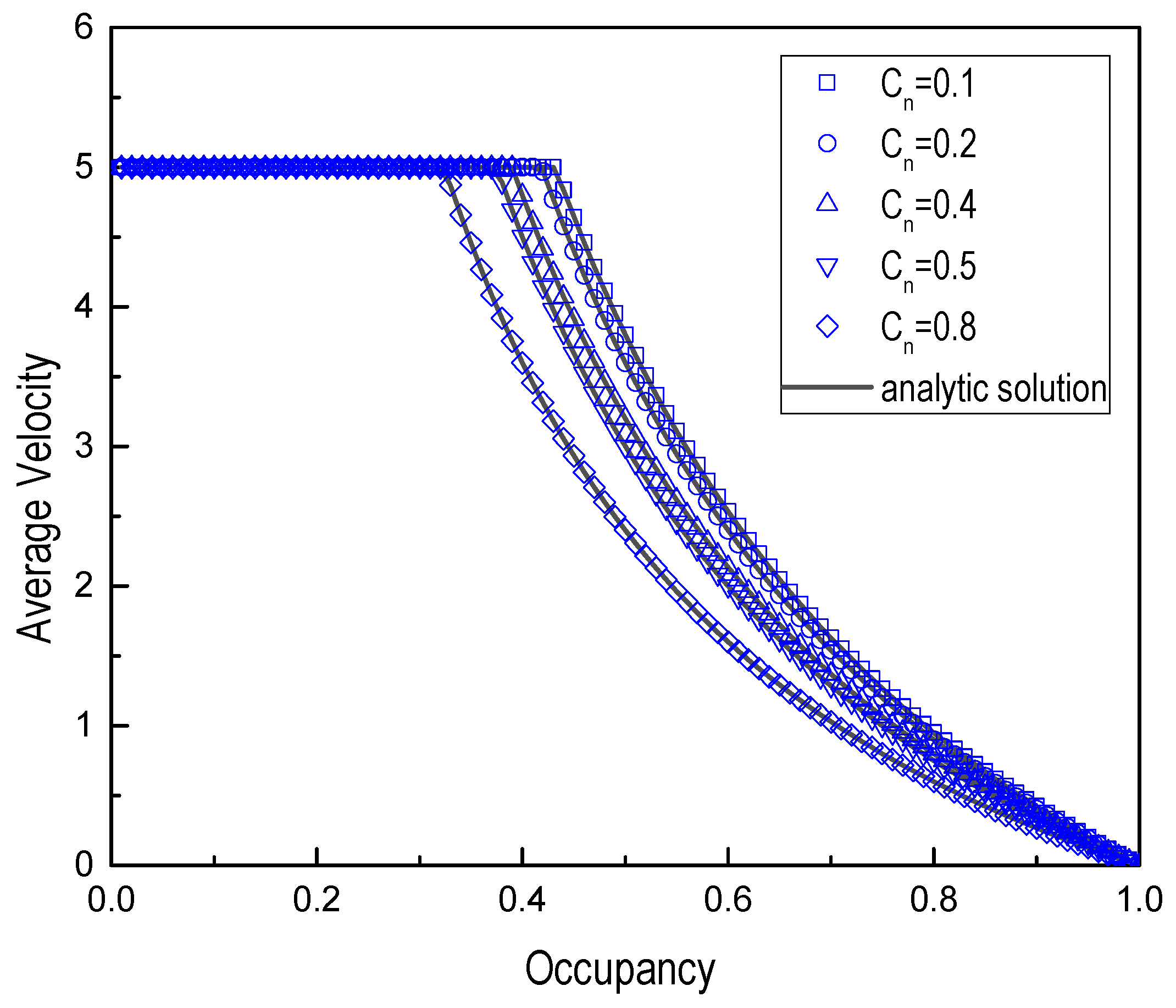
Firstly, the fundamental diagrams of mixed traffic flow are studied for different mixing ratios, C n . The mixed traffic flow on the road is composed of vehicles with different vehicle lengths and the maximum velocity in terms of the mixing ratio, C n . The long vehicle with the maximum velocity V L max = 10 occupies two cells and the short vehicle with the maximum velocity V S max = 5 occupies one cell at the initial moment. Thus, V max = min ( V L max , V S max ) = 5. The fundamental diagrams and average vehicle velocity vs. occupancy, C, of mixed traffic flow with mixing ratios C n = 0.1, 0.2, 0.4, 0.5, and 0.8 are shown in Figure 3 and Figure 4, respectively.
As can be seen from Figure 3 and Figure 4, the numerical simulation was consistent with the analytical solution. Traffic flow was proportional to occupancy, C, in the free flow and decreases with occupancy, C, in the congested state. Because of the rise in mixing ratio, Cn, the increase of short vehicles will lead to traffic jams easily. Moreover, when the occupancy is small, Figure 3 displays that the flow rate has different slopes due to the mixing ratio, Cn. In the case of traffic congestion, the flow rate slope was the same and had nothing to do with the mixing ratio, Cn. The curves in Figure 3 merged into a line whose slope is −2. These numerical simulations were in good agreement with Equation (25) obtained from the theoretical analysis.

3.2.2. Effect of Vehicle Length on Mixed Traffic Flow

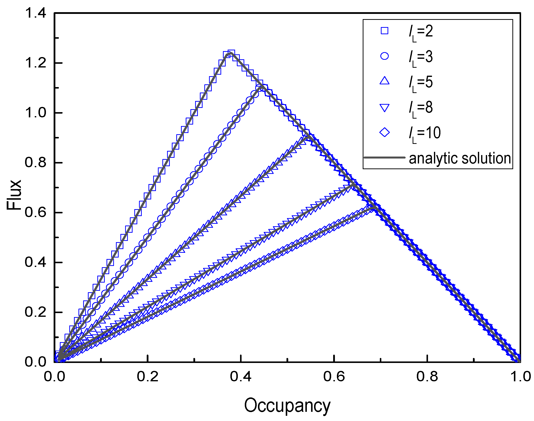
To study the effect of different lengths of vehicles on mixed traffic flow, we changed the length of the long vehicle and kept the short vehicle length constant (lS = 1). The maximum velocities of the long vehicle and short vehicle were, respectively selected as V L max = 10 and V S max = 5 and the mixing ratio Cn = 0.5. Figure 5 and Figure 6 show the fundamental diagrams and average velocity for long vehicle length lL = 2, 3, 5, 8, and 10 cells, respectively. All figures show that the numerical simulation was in agreement with the analytical solution.
As can be seen from Figure 5 and Figure 6, it was more impossible to cause traffic congestion with the increase of the length of the long vehicle due to the jamming transition point in the mixed traffic flow increasing in terms of Equation (20).

3.2.3. Effect of the Maximum Velocity on Mixed Traffic Flow

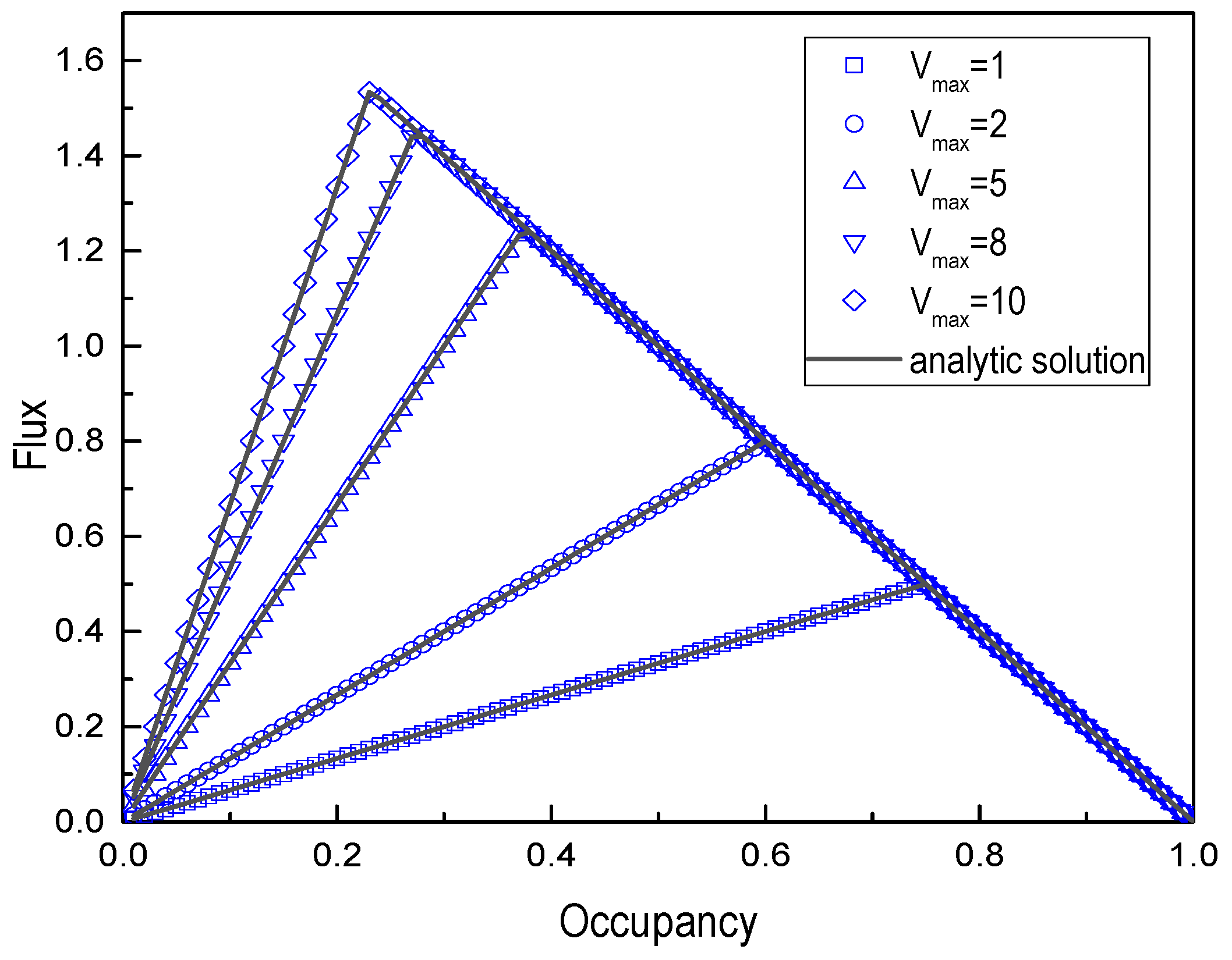
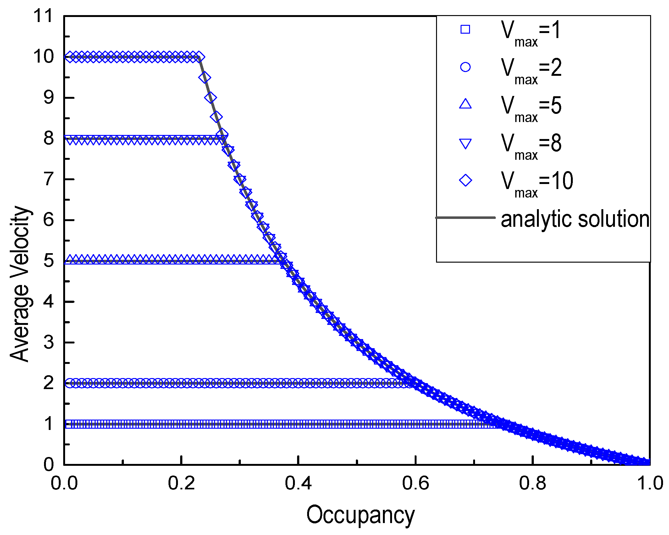
Similarly, we changed the maximum velocity of the short vehicle and fixed the maximum velocity of long vehicles to study the effect of the maximum velocity of mixed traffic flow. The length of the longest vehicle and the maximum velocity were, respectively selected as lL = 2 cells and V L max = 10. Accordingly, the mix ratio was C n = 0.5. In the same way, Figure 7 and Figure 8 show the fundamental diagram and average vehicle velocity vs. occupancy for different maximum velocities of the short vehicle, V S max = 1, 2, 5, 8, and 10.
Results also show that the numerical simulation is well in agreement with the analytical solution. The higher the maximum velocity of a short vehicle, the more likely it is to cause traffic jams.

4. Conclusions

Based on a one-dimensional (1D) cellular automaton (CA) FI model of traffic flow, we proposed a deterministic extended one-dimensional cellular automaton FI model, called the NIFI model, with consideration of the next-nearest-neighbor interaction. Using the mean-field analysis, the analytic solution of the NIFI model in one-dimensional single traffic flow was derived under periodic boundary conditions. Compared with the original deterministic FI model, the jamming transition between the freely moving and jammed phases occurred at a higher density when the next-nearest-neighbor interaction was considered. For the mixed traffic flow, we introduced the mixing ratio, C n , and the occupancy, C, to replace the vehicle density, ρ . Similarly, using the mean-field theory, the analytic solution of the mixed traffic flow was derived from the long-time evolution to reach the steady state. To verify the solutions, we conducted numerical simulations for the mixed traffic flow composed of different vehicle lengths, maximum velocities, and mixing ratios. All numerical simulations indicated that the numerical simulation results and the analytical solutions were matched excellently. Moreover, the vehicle length, the maximum velocity, and the mixing ratio had a great impact on the mixed traffic flow. However, there are still some limitations in our research. The NIFI model is a deterministic model, ignoring the stochastic delay scenario in nearest-neighbor and next-nearest-neighbor interactions. In future studies, the stochastic FI model considering the next-nearest neighbor interaction can be used as a research topic.
Although the NIFI model is a quite simple one-dimensional cellular automata model of traffic flow, the study of the interaction of the next-nearest-neighbor is helpful to anticipate the dynamic behavior of vehicles resulting in the stabilization of traffic systems. Therefore, it may be used in the forecast of traffic flow and traffic management in the future.

Author Contributions

Conceptualization, Y.Z., Y.X. and B.C.; methodology, Y.Z. and Y.X.; validation, Y.Q. and B.C.; formal analysis, Y.Z., Y.X. and Y.Q.; investigation, Y.Z., Y.X. and B.C.; data curation, Y.Z., Y.X. and Y.Q.; writing—original draft preparation, Y.Z.; writing—review and editing, Y.Z., Y.X. and Y.Q.; visualization, Y.Z., Y.X. and B.C.; supervision, Y.Z., Y.X. and B.C.; project administration, Y.Z., Y.X. and Y.Q. All authors have read and agreed to the published version of the manuscript.

Funding

This research is supported by the National Natural Science Foundation of China (Grant No. 11962002); the Natural Science Foundation of Guangxi, China (Grant No. 2018GXNSFAA138205); and the Innovation Project of Guangxi Graduate Education (Grant No. YCBZ2021021).

Institutional Review Board Statement

Not applicable.

Informed Consent Statement

Not applicable.

Data Availability Statement

All data generated or analyzed during this study are included in this article.

Conflicts of Interest

The authors declare no conflict of interest.

References

  1. Chowdhury, D.; Santen, L.; Schadschneider, A. Statistical physics of vehicular traffic and some related systems. Phys. Rep. 2000, 329, 199–329. [Google Scholar] [CrossRef] [Green Version]
  2. Wolfram, S. Theory and Applications of Cellular Automata; World Scientific: Singapore, 1986. [Google Scholar]
  3. Nagel, K.; Schreckenberg, M. A cellular automaton model for freeway traffic. J. Phys. I 1992, 2, 2221–2229. [Google Scholar] [CrossRef]
  4. Biham, O.; Middleton, A.A.; Levine, D. Self-organization and a dynamical transition in traffic-flow models. Phys. Rev. A 1992, 46, 6124–6135. [Google Scholar] [CrossRef] [PubMed] [Green Version]
  5. Fukui, M.; Ishibashi, Y. Traffic Flow in 1D Cellular Automaton Model Including Cars Moving with High Velocity. J. Phys. Soc. Jpn. 1996, 65, 1868–1876. [Google Scholar] [CrossRef]
  6. Kerner, S.B. Physics of automated driving in framework of three-phase traffic theory. Phys. Rev. E 2018, 97, 042303. [Google Scholar] [CrossRef]
  7. Madani, A.; Moussa, N. Simulation of fuel consumption and engine pollutant in cellular automaton. J. Theor. Appl. Inf. Technol. 2012, 35, 250–257. [Google Scholar]
  8. Lakouari, N.; Oubram, O.; Bassam, A.; Hernandez, S.E.P.; Marzoug, R.; Ez-Zahraouy, H. Modeling and simulation of CO2 emissions in roundabout intersection. J. Comput. Sci. 2020, 40, 101072. [Google Scholar] [CrossRef]
  9. Wang, X.; Xue, Y.; Cen, B.L.; Zhang, P. Study on pollutant emissions of mixed traffic flow in cellular automaton. Phys. A 2020, 537, 122686. [Google Scholar] [CrossRef]
  10. Qiao, Y.F.; Xue, Y.; Wang, X.; Cen, B.L.; Wang, Y.; Pan, W.; Zhang, Y.X. Investigation of PM emissions in cellular automata model with slow-to-start effect. Phys. A 2021, 574, 125996. [Google Scholar] [CrossRef]
  11. Chauhan, S.; Kumar, L. Survey Paper on Traffic Flow Control using Cellular Automata. Int. J. IT Eng. Appl. Sci. 2013, 2, 1–7. [Google Scholar]
  12. Das, D.; Misra, R. Improvised dynamic network connectivity model for Vehicular Ad-Hoc Networks (VANETs). J. Netw. Comput. Appl. 2018, 122, 107–114. [Google Scholar] [CrossRef]
  13. Barlovic, R.; Santen, L.; Schadschneider, A.; Schreckenberg, M. Metastable States in Cellular Automata for Traffic Flow. Eur. Phys. J. B 1998, 5, 793–800. [Google Scholar] [CrossRef] [Green Version]
  14. Wang, B.H.; Wang, L.; Hui, P.M.; Hu, B. Analytical Results For The Steady State Of Traffic Flow Models With Stochastic Delay. Phys. Rev. E 1998, 58, 2876–2890. [Google Scholar] [CrossRef] [Green Version]
  15. Wang, L.; Wang, B.H.; Hui, P.M. Strict derivation of mean-field equation for one-dimensional traffic flow model. Acta Phys. Sin. Overseas Ed. 1997, 6, 829–836. [Google Scholar]
  16. Wang, B.H.; Wang, L.; Hui, P.M. One-dimensional Fukui-Ishibashi traffic flow model. J. Phys. Soc. Jpn. 1997, 66, 3683–3684. [Google Scholar] [CrossRef]
  17. Wang, B.H.; Wang, L.; Hui, P.M.; Hu, B. The asymptotic steady states of deterministic one-dimensional traffic flow models. Phys. B Condens. Matter 2000, 279, 237–240. [Google Scholar] [CrossRef]
  18. Fu, C.J.; Wang, B.H.; Yin, C.Y.; Zhou, T.; Hu, B.; Gao, K.; Hui, P.M.; Hu, C.K. Analytical studies on a modified Nagel–Schreckenberg model with the Fukui–Ishibashi acceleration rule. Chaos Solitons Fractals 2007, 31, 772–776. [Google Scholar] [CrossRef] [Green Version]
  19. Jia, N.; Ma, S. Analytical results of the Nagel-Schreckenberg model with stochastic open boundary conditions. Phys. Rev. E 2009, 80, 041105. [Google Scholar] [CrossRef]
  20. Jia, N.; Ma, S. Analytical investigation of the open boundary conditions in the Nagel-Schreckenberg model. Phys. Rev. E 2009, 79, 031115. [Google Scholar] [CrossRef]
  21. Ding, Z.J.; Jiang, R.; Wang, B.H. Traffic flow in the Biham-Middleton-Levine model with random update rule. Phys. Rev. E 2011, 83, 047101. [Google Scholar] [CrossRef]
  22. Ding, Z.; Liu, T.; Lou, X.; Shen, Z.; Zhu, K.; Jiang, R.; Wang, B.; Chen, B. Mean-field analysis for Asymmetric Exclusion Processes on two parallel lattices with fully parallel dynamics. Phys. A 2018, 516, 317–326. [Google Scholar] [CrossRef]
  23. Nagatani, T. Stabilization and enhancement of traffic flow by the next-nearest-neighbor interaction. Phys. Rev. E 1999, 60, 6395–6401. [Google Scholar] [CrossRef] [PubMed] [Green Version]
  24. Li, X.B.; Jiang, R.; Wu, Q.S. Cellular automata model simulating complex spatiotemporal structure of wide jams. Phys. Rev. E 2003, 68, 016117. [Google Scholar] [CrossRef] [PubMed]
  25. Ge, H.X.; Dai, S.Q.; Dong, L.Y.; Xue, Y. Stabilization effect of traffic flow in an extended car-following model based on an intelligent transportation system application. Phys. Rev. E 2004, 70, 066134. [Google Scholar] [CrossRef] [PubMed]
  26. Chowdhury, D.; Wolf, D.E.; Schreckenberg, M. Particle hopping models for two-lane traffic with two kinds of vehicles: Effects of lane-changing rules. Phys. A 1997, 235, 417–439. [Google Scholar] [CrossRef]
  27. Knospe, W.; Santen, L.; Schadschneider, A.; Schreckenberg, M. Disorder effects in cellular automata for two-lane traffic. Phys. A 1999, 265, 614–633. [Google Scholar] [CrossRef] [Green Version]
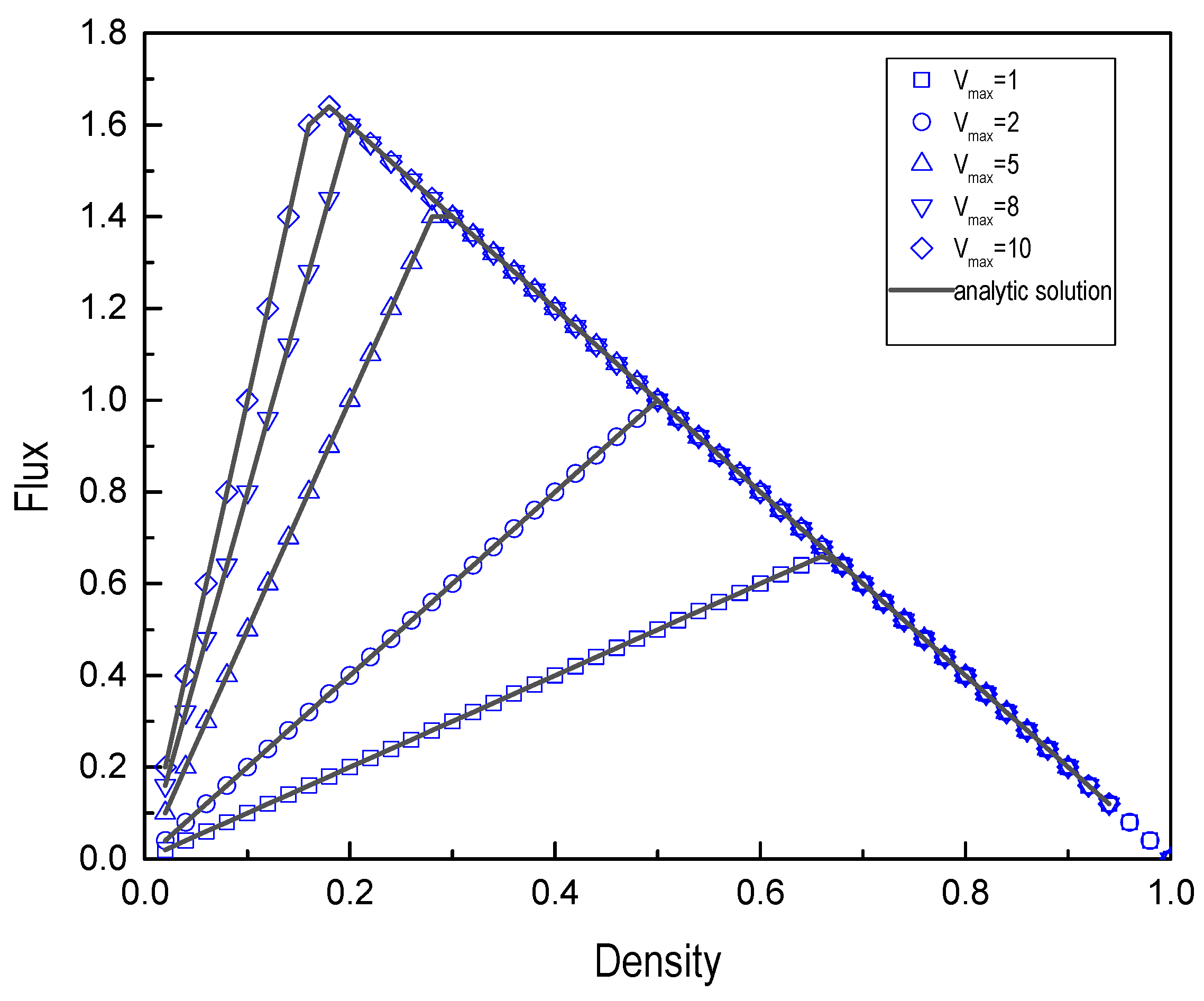
Figure 1. Fundamental diagram for different maximum velocity.
Sustainability 14 07127 g001
Figure 2. Average velocity vs. density for different maximum velocity.
Sustainability 14 07127 g002
Figure 3. Fundamental diagram for different mixing ratios (lS = 1 cell, lL = 2 cells, V L max = 10 and V S max = 5).
Sustainability 14 07127 g003
Figure 4. Average velocity vs. Occupancy, C, for different mixing ratios (lS = 1 cell, lL = 2 cells, V L max = 10 and V S max = 5).
Sustainability 14 07127 g004
Figure 5. Fundamental diagram for different lengths of vehicle (lS = 1 cell, Cn = 0.5, V L max = 10 and V S max = 5).
Sustainability 14 07127 g005
Figure 6. Average velocity vs. Occupancy, C, for different lengths of vehicle (lS = 1 cell, Cn = 0.5, V L max = 10 and V S max = 5).
Sustainability 14 07127 g006
Figure 7. Fundamental diagram for different maximum velocities (lS = 1 cell, lL = 2 cells, Cn = 0.5 and V L max = 10).
Sustainability 14 07127 g007
Figure 8. Average velocity vs. Occupancy for different maximum velocities (lS = 1 cell, lL = 2 cells, Cn = 0.5 and V L max = 10).
Sustainability 14 07127 g008
Publisher’s Note: MDPI stays neutral with regard to jurisdictional claims in published maps and institutional affiliations.