Abstract
Taxis are an important component of the urban public transportation system, with wide geographical coverage and on-demand services characteristics. Thorough understanding of the built environment affecting taxi ridership can enable transportation authorities to develop targeted policies for transportation planning. Previous studies in this field had few data sources and did not consider the spatiotemporal variability. This study aims to develop an analytical framework for understanding the spatiotemporal correlation between the urban built environment and taxi ridership, which is empirically analyzed in New York City. The built environment is defined through multisource data in terms of density, design, diversity, and destination accessibility. Besides the exploration of travel patterns, the spatiotemporal heterogeneity of taxi ridership is modeled using geographically and temporally weighted regression (GTWR). The result shows that GTWR outperforms ordinary least squares (OLS), geographically weighted regression (GWR), and temporally weighted regression (TWR) in both goodness of fit and explanatory accuracy. More importantly, our study found that land use diversity is negatively correlated with taxi ridership, while transportation diversity is positively correlated with it. A highly accessible road network improves the people’s demand for taxis in the morning rush hours. Moreover, the density of railway stations is positively correlated with taxi ridership on weekdays but adversely on weekends. These findings provide practical insights for urban transportation policy development and taxicab regulation.
1. Introduction
In recent years, rapidly growing travel demand has led to road congestion, air pollution, and even traffic accidents, which is essentially the result of the supply and demand imbalance between the travel demand and the urban infrastructure. A possible way to alleviate this problem is to discover the people’s travel preferences for different built environment distributions. The built environment emphasizes the function and infrastructure of urban sites, and it has already been proven to have a significant impact on transit ridership [,]. In addition, taxi is a mode of transit in high demand, geographically spread, and with door-to-door services []. A thorough understanding of the built environment factors affecting taxi ridership can enable transportation authorities to effectively develop targeted policies for allocating limited transit resources and alleviating the crowd traffic.
In the past decades, studies on the built environment-influencing factors of taxi ridership can be divided into several dimensions, with most studies focused on the density of points of interest (POIs), public transit stops, and the design of the road network. They found factors associated with taxi ridership based on regression models, and a significant portion took into account the spatial heterogeneity of travel demand in recent years [,,]. So far, several findings have been revealed and widely recognized in the existing studies. For urban land use functions, taxi demand is higher in developed areas with dense distribution of residential and commercial sites and a high degree of mixed land use [,]. In addition, a positive correlation between scenic area density and taxi usage rate on weekends was found []. In response to the effect of other transportation modes on taxi ridership, it has been proven that the taxi demand is lower in areas with more bus stops [] and higher in areas with more railway stations []. Tang also observed that the higher the accessibility of other transit modes, the more likely it is to mismatch the taxi distribution []. At the same time, there have been a few studies that analyzed the impact of road network design on taxi ridership, such as taxi demand being higher in areas with well-developed arterial roads and dense secondary roads [,]. These findings have made progress in revealing the people’s travel preferences by taxi in different built environment distributions.
However, there are still some uncertainties in this area. From people’s perspective, offering a diversity of public transit modes can reduce taxi ridership due to people preferring to travel with less travel time and cost. At the same time, the placement of more diverse transit facilities also implies that there is a large demand for travel in a given location, resulting in an uncertain correlation with taxi ridership. Similarly, a high mixed land function development always leads to high travel demand, while also resulting in short travel distances [,], which possibly makes people less reliant on taxis. These perspectives reflect the incompleteness of the existing studies. Further, the density of the road network only reflects the macrolevel urban planning; how does its accessibility affect taxi ridership? How the impact of the built environment on taxi ridership varies in the spatial and temporal dimensions? These unanswered questions in the existing studies make it difficult for transportation authorities to make effective decisions based solely on the few dimension analyses of the existing studies.
In summary, the existing studies have explored the travel demand determinants by some factors. However, few efforts have been made to explore taxi travel demand-influencing factors at an aggregate level from the spatial and temporal perspectives, in particular the correlation between taxi ridership and the built environment. In addition, besides the density of POIs [,], limited studies have considered multiple dimensions of the built environment with spatiotemporal heterogeneity. To fill these gaps, this study aims to develop an analytical framework to reveal the influence of the built environment on taxi ridership based on multisource data, which was empirically analyzed in New York City. First, the multisource built environment in terms of density, design, diversity, and destination accessibility was defined in the modeling process. Further, we established GTWR in the correlation analysis between the built environment and taxi ridership, which was able to deal with the spatiotemporal heterogeneity of variables. Finally, we illustrated the distribution of taxi travel patterns and revealed the determinant factors of taxis in built environments from the spatiotemporal perspective. More importantly, our study found that land use diversity is negatively correlated with taxi ridership, while transportation diversity is positively correlated with it. A highly accessible road network improves the people’s demand for taxis in the morning rush hours and reduces it mostly downtown. These findings generate previously unobtainable insights for policy development of urban and transportation planning.
The remainder of the paper is organized as follows. Section 2 reviews the existing methodologies and findings between the built environment and taxi ridership. Section 3 describes the study area, data sources, and processing of the datasets. Section 4 presents the methods of explanatory variables definition, multicollinearity judgment, spatiotemporal nonstationarity, and regression modeling. Section 5 provides the results and the discussion of travel patterns and correlation analysis. In Section 6, we summarized the conclusions and provided suggestions for urban and transportation planning.
2. Literature Review
2.1. Factors Affecting Transit Ridership
Exploring the factors that influence people’s travel activities is important for urban planning and transportation policy development. In the previous studies, the factors related to travel behavior can be summarized into several dimensions: weather, economic, sociodemographic, and built environment. The economic factors measure the impact of regional development levels on travel demand []. The sociodemographic factors emphasize the correlation between the ethnicity, age, income, education, and employment rate of people on travel behavior, aim to discover the travel preferences of people [,]. The built environment focuses on the impact of land use function and urban infrastructure on travel behavior. Planning of the built environment influences travel patterns (travel time, frequency, mode, route choice, etc.) by configuring the functions of urban parcels, thus guiding the balanced distribution of traffic flows in the road network []. Several studies have recognized the important contribution of the built environment to the influence of travel demand [,,]. In the past decades, these influencing factors were mainly obtained through travel surveys or questionnaires with insufficient data samples and inherent sampling bias, which directly led to the lack of credibility of the analytical results []. In recent years, the development of data sensors has provided access to high-precision and large-scale multisource data, such as remotely sensed land use data and GPS data [], which gives support to revealing the influencing factors of transportation ridership at the regional level.
2.2. Methodologies
2.2.1. Global Perspective
Quantifying the impact of the built environment on travel demand is an ongoing challenge in the transportation analysis field. Linear regression, the most representative method in correlation analysis, has been widely used in the modeling between travel demand and the built environment [,]. It uses the OLS model to solve the unknown coefficients, which is comprehensible, computationally inexpensive, and can produce coefficient estimations for the entire study area. However, there is significant spatial heterogeneity in the travel demand of people due to different land development intensities and functions in urban areas []. The regression coefficients derived from OLS can be considered the result of ‘averaging’ multiple subregions within the analyzed area. Its low fitting accuracy and insufficient explanatory power for travel demand were criticized in the previous studies [,].
For analysis from a global perspective, structural equation modeling (SEM) has been preferred due to its advantage of dealing with multiple dependent variables simultaneously []. It has been employed in exploring the built environment’s impact on multiple modes of transportation []. In addition, binomial regression and logistic regression have been applied to model the correlation analysis of travel behavior. Yu [] revealed that in urban villages in China, mixed land use decreases public transport ridership. Hochmair [] found that rail transit was positively correlated with the number of taxi trips using the nonspatial binomial regression model, and this effect became statistically insignificant when a spatially filtered binomial regression model was applied, which illustrated the spatial variation of the travel demand. Sabouri [] also emphasized the importance of incorporating spatial characteristics into the analysis of travel demand correlation.
2.2.2. Spatial and Temporal Perspective
To improve the above situation, the spatial lag model [,], GeoDetector [], and GWR [] were applied to take into account the spatial heterogeneity of travel demand. GWR introduced a kernel function based on spatial distance into the regression process and has been most widely used. Qian [] applied GWR to deal with spatial heterogeneity and found evidence of a positive correlation between subway accessibility and taxi ridership. Tang [] employed GWR to capture the spatial nonstationarity of taxi ridership and identified the key influencing factors by introducing a generalized linear model. Later, the advantages of improved models based on GWR in the field of travel behavior have been discovered. GWPR was applied to explore the correlation between ride-sourcing demand and the built environment based on the Poisson distribution of the dependent variable []. Chen [] improved the Euclidean distance metric in traditional GWR to the Minkowski distance, which applied to the correlation analysis between the built environment and subway ridership, and demonstrated excellent goodness of fit compared to OLS and GWR.
In recent years, temporal characteristics have gradually been considered in correlation modeling, due to people traveling for different purposes at different times. Yu [] found that the built environment has a strong influence on cycling demand, with significant temporal heterogeneity. Liu [] introduced time dependence into a generalized additive model and found that taxi demand was higher in developed areas and areas with dense secondary roads and lower in areas with more bus stops. In recent years, travel demand correlations that simultaneously considered spatiotemporal characteristics have been innovatively applied by GTWR. GTWR was innovated traditional GWR by quantifying the spatiotemporal distance in the regression process, which was first proposed and applied in the correlation analysis of housing prices []. In 2018, GTWR was first introduced into transportation-influencing factors modeling []. However, these studies focused on bus and subway ridership [] or bicycle-sharing systems [], for which travel modes feature fixed stops or short distances. In addition, they only considered limited dimensions of factors, such as the density of POIs [], which is not sufficient for urban transportation policy implications.
3. Study Area and Data
3.1. Study Area
New York City (NYC) is the largest city in the United States and one of the largest metropolitan areas in the world, covering 300.46 square miles with a population of 8,804,190 as of 2020, along with well-developed urban public transportation facilities. In 2020, New York was rated Alpha++ by Globalization and World Cities Research Network as a Tier 1 World City []; its development directly affects the global economy, finance, media, politics, and other areas. The NYC region consists of five boroughs containing Manhattan, Brooklyn, Queens, Bronx, and Staten Island (Figure 1). Manhattan is the most densely populated area with the smallest footprint in NYC, is known as the economic center of the world, and its interior is usually divided into five major neighborhoods according to geographic location (Figure 1). With the same fare structure, NYC taxis are available in yellow and green, with additional taxes and fees for all trips. Green taxis are only able to carry passengers in Upper Manhattan, Brooklyn, Queens, and Staten Island, which were introduced in August 2013 to alleviate the lack of cab service in the outskirts. They are operated by private companies and regulated by the NYC Taxi and Limousine Commission (TLC). Due to competition with ride sharing, the number of passengers traveling by taxi has been declining year after year, but taxi remains one of the typical modes of public transportation under random travel behavior. The NYC taxi zones with yellow and green taxis are utilized as the analytical units in this study, including 263 traffic analysis zones (TAZs), which are roughly based on the NYC Department of City Planning’s Neighborhood Tabulation Area.
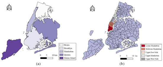
Figure 1.
Map and TAZs distribution of NYC. (a) NYC boroughs; (b) NYC taxi zones.
3.2. Data Description and Preprocessing
The travel demand data applied to this study were obtained from the TLC’s publicly available trip records datasets for both yellow and green taxis. The original travel records contain pick-up and drop-off timestamps, longitude, latitude, travel distance, number of passengers, fare, tax fees, and payment information. One week of data from 6 June 2016, to 12 June 2016, was employed in this study. Trip records with outliers and falling outside the study area were removed. Further, the OD matrix was obtained by mapping the OD points to the analytical units. The final processed data contain 2,005,334 records for weekdays and 775,836 records for weekends, including the information on pick-up and drop-off times, travel distance, travel time, and the cell ID for OD pairs (Table 1).

Table 1.
Sheet of processed trip record data.
Multisource data about the built environment employed in this study were from the Open Street Map geographic datasets. Specifically, POIs of land use, transportation facility points, railway network, and road network with the shapefile format were applied for preprocessing in ArcGIS. Different types of point and line geographic data were filtered based on fields, which were removed when falling outside the study area. Then, the processed data were classified and mapped into spatial analytical units for calculations.
Ewing [] summarized travel behavior is associated with the five ‘Ds’ of the built environment from the previous literature, including density, design, diversity, destination accessibility, and distance to transit. Due to the limitation of the datasets, four items were chosen in this study; their descriptions are shown in Table 2. After removing the variables with multicollinearity (mentioned in Section 4.2), a total of 21 explanatory variables were included in the dataset. Furthermore, the travel time and taxi flow in the TLC datasets were employed to define the explanatory variable of road network accessibility on weekdays and weekends.
Table 2.
The four “Ds” built environment and the information on the influencing factors.
The average travel demand per hour was calculated as dependent variables for weekdays and weekends, respectively. That is, for weekdays, the travel demand per hour is the average of the same period of five days, while for weekends, it is the average of the same period of two days. Overall, 263 TAZs with a 24 h dataset were input into GTWR, which was able to reflect the variation pattern of influencing factors in the whole area within 24 h.
4. Materials and Methods
4.1. Explanatory Variables
The analysis of GTWR is based on the available explanatory variable datasets in spatiotemporal analytical units, so there is a required calculation process of samples in each TAZ. The POI density indicates the amount of POIs per km2 in each TAZ; for the kth POI class of , it is calculated as follows:
where is the number of POIs of k class in and is the area of .
The density of road and railway networks means the line length proportion of an area; it reflects the development degree of the line network in the urban transportation system. Given a spatial analytical unit , the density of the line network is calculated as follows:
where is the type index of the line element which includes roads and railways in this study and is the length of the road or railway network in .
Differently from the study of the spatiotemporal influence of travel demand by GTWR, we first introduced the entropy of the built environment in explanatory variables based on the definition of information entropy [] and divided it into two categories, that is, the entropy of land use and transportation. Compared with the density of various POIs, their entropy can better reflect the impact of the layout of the built environment on travel behavior. Similarly to the idea of entropy, there is a larger value when there are more diverse land use functions or transportation modes in a spatial area and vice versa. Given the type of entropy index m, the spatial entropy of POIs in is described as follows:
where m represents the land use or the transport in this study, K denotes the number of POI types belonging to m; taking land use entropy as an example, indicates the amount of POIs with the kth type belonging to m which falls in and is the total amount of POIs belonging to m in , thereby means the quantity ratio of the kth category within m in . The higher the entropy value, the smaller the difference in the number of functional types.
The travel time of the transportation has a great influence on the choice of the travel mode and departure time of people; a more congested road network will reduce unnecessary travel or adopt other travel modes with less time spent [,]. For the overall urban road network, roads with different traffic flows have different contributions, and roads with heavy traffic have a greater impact []. Here, we introduce accessibility of the road network with weighted traffic flow and travel time of people to reflect the accessibility of :
where , indicates the average travel time from to and J means the number of TAZs, excluding ; represents the traffic volume from to . The less the weighted average travel time spent by people from , the higher the road network accessibility in it. It is an effective method of comparing the degree of convenience between different areas.
Accessibility of transportation measures the degree of convenience from the traffic station to the destination. In most recent studies, public transportation accessibility has been measured in different ways, including topological, contiguous, cumulative opportunities, utility, and flow-based measurements []. Due to intuitiveness and comprehensibility, we utilized the cumulative opportunity method [,] to quantify the accessibility of public transportation. It measures the number of opportunities that can be approached under the predefined travel impedance. In this study, the distance is used as travel impedance, which represents the acceptable walking distance from/to transit stops or stations, and the opportunities represent the POIs. That is, transportation accessibility measures the number of POIs that people can approach at a fixed distance. The 400 m buffer for bus stops and 800 m buffer for railway stations were selected in this section, which were commonly used in previous studies [,]. Public transportation accessibility is defined as follows:
where is the number of buffers that falls in and represents the number of POIs within buffer b in . It measures the average number of POIs that can be accessed on the way to transit stops.
4.2. Multicollinearity
The Pearson correlation coefficient and the variance inflation factor (VIF) were applied to determine the relationship between explanatory variables. To eliminate the error effects of variables multicollinearity on GTWR, the explanatory variables larger than 0.8 for the Pearson correlation coefficient or 8 for the VIF were removed from the following analysis. Specifically, the coefficient between shopping and catering was 0.868, and the accessibility of bus stops and subway stations reached 0.899. The results of the VIF are shown in Table 2. There are 21 explanatory variables of the built environment applied in GTWR after excluding the catering and subway accessibility.
4.3. Spatiotemporal Nonstationarity
GTWR has a great performance in revealing the built environment’s influence on travel demand when variables have the property of spatiotemporal heterogeneity. It can be judged by the interquartile range of GTWR estimation coefficients and standard errors (SE) of OLS [,,]. If the interquartile range of GTWR is larger than two times SE in OLS, it is demonstrable that there is spatiotemporal nonstationarity of variables. The results are shown in Table 3. All the explanatory variables have extra local variation and are suitable for the following analysis by GTWR.
Table 3.
The spatiotemporal nonstationarity test of explanatory variables.
4.4. Regression Models
Regression models have been proved to be important means of discovering correlated factors of travel behavior [,,]. Linear regression models are calculated from a global perspective and estimate the unknown parameters using the OLS model [], while GWR introduces the spatial nonstationarity property into the regression process [,]. It is critical to emphasize that travel demand exhibits significant dynamic characteristics in both time and space. Thereby, capturing spatiotemporal heterogeneity in regression models simultaneously proved to be effective. Huang [] proposed the GTWR model based on GWR, which corrected the weights by introducing spatiotemporal distance and could achieve fast conversion between GWR, TWR, and GTWR models based on the parameters adjustment. It has significant advantages in dealing with correlation analysis under spatiotemporal dynamic datasets and is suitable for travel behavior analysis in urban transportation [,]. Here, we present a short review of the theoretical modeling approaches of OLS, GWR, TWR, GTWR and employ them for comparative analysis of taxi ridership and built environment correlations under multisource data.
The OLS model has been widely used in the analysis of influencing factors of travel behavior [,]. However, the coefficients generated by OLS can be seen as the result of averaging across geographic locations, it has unsatisfied explanatory powers since the variables have an obvious character of nonstationarity over space []. GWR was introduced to solve this problem []. It extends the OLS regression model by introducing geographic variation to the model coefficients’ estimation. The form of the GWR model is introduced as follows:
where , and is the intercept and error of in , respectively; denotes the coefficient of the k explanatory variable, while indicates the samples of the k explanatory variable in . It utilizes the weighted least squares for the estimation of the unknown coefficients, which are calculated as follows:
where is the weighted spatial distance matrix which is calculated using a kernel function. Its diagonal values are the weighted distance for , while the remaining values are filled with 0. The Gaussian kernel function is commonly utilized in this period [], then the weighted value between and can be calculated as follows:
where if Euclidean distance is applied, and h is the optimal bandwidth in GWR []. It can be understood that GWR calibrates the individual regression models for each location by combining data from the nearby locations and weighting them according to the distance from the regression point. If the values are from locations closer to the regression point, they will be weighted more than from the locations farther away from the regression point.
Huang [] proposed GTWR which can capture spatial and temporal heterogeneity simultaneously. For , GTWR can be expressed as follows:
where and are the intercept and coefficient in at observation time t. Similarly, the estimated coefficients can be represented as follows:
Differently from the GWR model, denotes the spatiotemporal distance matrix via the kernel function. If the Euclidean distance and the Gaussian kernel function are applied in GTWR, between and can be calculated as follows:
where and , respectively; denotes the spatiotemporal bandwidth and , . GTWR fuses spatial and temporal distances by weighted and in . If is set to 0, then the time distance is removed from GTWR, it is degraded to the GWR model. If , only the temporal nonstationarity can be captured, which is considered TWR []. The spatiotemporal distance in GTWR can be simplified as follows:
where in the distance definition, which balances the spatial and temporal distance in GTWR.
The optimization of bandwidth is commonly achieved by minimizing the value of cross-validation (CV) or the corrected Akaike information criterion (AIC) in GWR-based models [,]. Here, the CV approach is applied to bandwidth calculation in this study. It is defined as follows:
where is the predicted value of from GTWR. The CV method finds the optimal bandwidth with the least sum of squares in the regression. All the regression models (OLS, GWR, TWR, GTWR) in this study were implemented using the GWmodel package in R [,].
5. Results and Discussion
5.1. Travel Patterns Comparison
The distribution of travel patterns is shown in Figure 2 and Figure 3, including travel distance and travel time comparison and distribution on weekdays and weekends. The average travel distance by taxi in NYC is 2.92 miles on weekdays and 3.05 miles on weekends. More than half of the travel distances are less than 2 miles, with more weekday trips included. People prefer medium- and long-distance trips between 2 miles and 8 miles on weekends, while trips on weekdays and weekends are similar in proportion when the distance is greater than 8 miles. Interestingly, although people travel shorter distances on weekdays, they spend more time on the trip compared to weekends. The average values of travel time on weekdays and weekends are 15.31 min and 13.01 min, respectively. In any case, most trips have a travel time of 5 to 10 min. The percentage of weekend trips is generally higher than on weekdays when the travel time is 15 min or less. However, the number of weekday trips consistently exceeds that of weekends when travel times are longer than 15 min. It is worth mentioning that a small percentage of trips on weekdays are longer than 1 h, while this phenomenon rarely occurs on weekends.
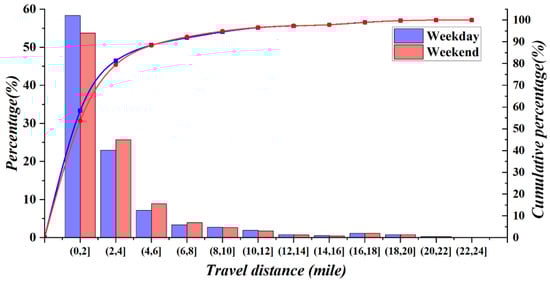
Figure 2.
Travel distance distribution on weekdays and weekends.
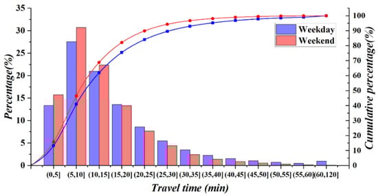
Figure 3.
Travel time distribution on weekdays and weekends.
The average values of travel time and distances in each TAZ are summarized in Figure 4. TAZs with dark red represent long average travel time or distances which taxis travel. Only a few trips originate from Staten Island. Due to the high density and diversity of the land use functions in Manhattan, most trips travel from there are always less than 3 miles, and in the north of the Upper Manhattan and the south of the Lower Manhattan, the travel distance increases. In addition, people tend to travel further on weekends, especially trips from Bronx and eastern areas of Queens. Overall, the further the departure TAZs are from the downtown areas, the longer the average travel distance and time will be. Furthermore, there are differences in travel time when traveling on weekdays and weekends, with travel time generally longer when traveling on weekdays. It may be caused by traffic congestion on roads especially in Manhattan and Brooklyn, while for the southern areas in Queens, the reason for the long travel time is more due to the long travel distances. People traveling from these remote areas always take an average of 20 min to 1 h, with average distances between 6 and 20 miles.
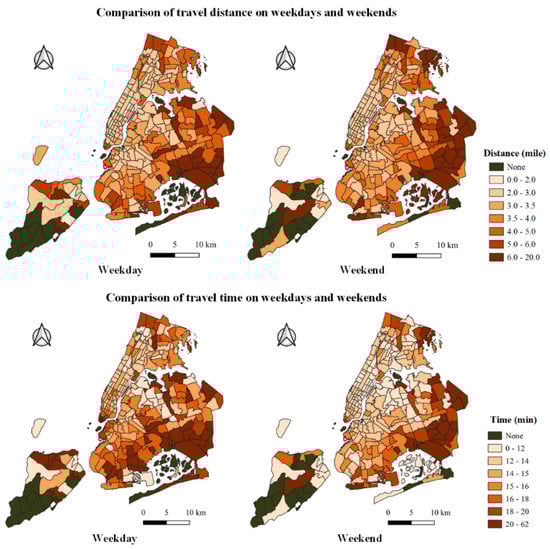
Figure 4.
Comparison of travel patterns on TAZs.
5.2. Model Results
Results for model comparisons of OLS, GWR, TWR, and GTWR are shown in Table 4. Models only considering spatial or temporal nonstationarity are effective, leading to a decrease in RSS, AIC, AICc, and an increase in R2 compared with OLS. We can see that GTWR has the most excellent performance in explaining the built environment’s influence on taxi ridership compared with others. When applied on weekdays, RSS decreases to 1,470,040, and R2 increases to 0.990, while on weekends, RSS and R2 are 813,424.9 and 0.993, respectively. The GTWR model can almost fully explain the influence of the built environment on traffic demand, and deal well with the spatiotemporal heterogeneity of the variables.
Table 4.
Comparisons of the regression models.
Coefficients of GTWR varied in spatiotemporal units; the results of the coefficients with weekdays and weekends are shown in Table A1 and Table A2 (Appendix A). The magnitude of the coefficient implies the significance of the effect of the variable on taxi ridership. Due to the limitation of space, we discuss only the representative results. Here, we analyzed the difference modes between weekdays and weekends by comparing the average coefficients (Table 5). In Table 5, we can see that there is a strong relationship between land use function and taxi ridership; e.g., high density of leisure, tourism, and worship places always leads to the increase in taxi demand on weekends while decreasing it on weekdays due to the difference in the purpose of people’s travel. For the travel modes of bus and railway, there is an interesting difference in the density of the two kinds of stations’ coefficients. The density of railway stations and the railway network has an overall positive correlation with taxi demand on weekdays, while the opposite is true on weekends. It is different from the study that only revealed more railway stations are associated with an increase in taxi trips []. This difference could be attributed to the relaxed time requirements and less spending on travel on weekends, which makes taxis unpopular compared with the railway. However, the bus is one of NYC’s well-developed modes of public transportation, while the density of its infrastructure has very little impact on the taxi ridership.
Table 5.
Average coefficients estimation on weekdays and weekends.
So far, there is no study on the correlation between transportation diversity and taxi ridership. Here, we fill this gap by quantifying the entropy of infrastructures of different travel modes. It is generally accepted that offering a variety of transportation options can reduce the ridership of a particular travel mode. At the same time, the placement of multimodal transportation facilities implies that there is a large demand for travel in a given location, resulting in an uncertain correlation with taxi ridership. According to Table 5, we found that the more alternative transportation modes, the more people travel by taxi, and there is hardly any difference between weekdays and weekends. This is possibly due to the fact that only a few modes of transportation can replace taxis when people travel relatively fixed distances, and the large travel demand plays an important role in increasing taxi ridership. We also found that there is a significant negative correlation between land use entropy and taxi trips, since planning for diverse land use functions encourages people to travel for shorter distances with fewer taxis, and it is also an effective way to alleviate road congestion [,,].
Surprisingly, according to the average coefficients of road network accessibility (Table 5), we found that the less travel time people spend, the less willing are people to travel by taxi. Furthermore, this variable has a different impact on taxi ridership for different peak hours of the week (Table A3, Appendix A). It can be seen that the shorter the travel time of trips, the less the demand for taxis during noon and the evening peak time and the higher in the morning rush hours. This indicates that during the morning peak of a working day, people value travel time more than in other periods.
The predicted travel demand using GTWR on weekdays and weekends is shown in Figure 5. GTWR can also be employed to predict future spatiotemporal variations of taxi demand with great performance. The kernel function with spatiotemporal distances makes the dependent variable change continuously over time, whereas it leads to insensitivity for abrupt values, such as the values at 8 am and 4 pm on weekdays. Comparing the two fluctuation modes of the average taxi ridership on weekdays and weekends, it can be seen that the peak time on weekends is always later than on weekdays, and there is more taxi ridership at midnight on weekends.
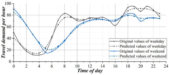
Figure 5.
Comparisons of the average original and predicted values of GTWR.
5.3. Temporal Features
The regression coefficients of GTWR in spatial units have differences in the temporal field compared with GWR. In this section, we analyze the variation of the regression coefficients over time by aggregating TAZs in representative districts and average the coefficients in temporal units. Manhattan is the most important borough of NYC with most trips generated from it []. A full analysis of Manhattan plays an important role in transportation policy development. As a result, two perspectives of coefficients’ variation of Manhattan were analyzed as follows: (a) temporal variation of coefficients has similar trends on weekdays and weekends; (b) temporal variation of coefficients has different trends on weekdays and weekends. Then, we emphasized the influencing factors of diversity in Manhattan, which are new factors introduced for GTWR in this study.
Temporal variation of coefficients has similar trends, which means the coefficient generates positive or negative influence on both weekdays and weekends and is always stronger during peak periods, for which the peak time definition is shown in Table A3, Appendix A. The average result of coefficients obtained from GTWR is displayed in Figure 6. A significant positive correlation is found between land use for education and taxi ridership for the morning peak period of weekdays. The high density of parking sites aggregates the demand for taxis strongly in Manhattan; this result is likely to be related to the highly diverse land use and dense population of the downtown []. Land use of tourism and public facilities also have positive correlations with taxi ridership, and as for tourism, there is a variation over time with a more obvious effect in the evening peak time on weekends.
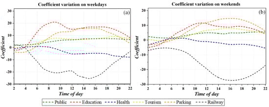
Figure 6.
Temporal variation of coefficients has similar trends. (a) Weekdays; (b) weekends.
An effective method that can reduce the demand for taxis is to increase the density of railway stations; it is more useful during rush hours of the week. Interestingly, there are also differences in the effect of the density of railway stations on taxi ridership in the morning and evening rush hours. Due to the relaxation of the travel time required in the evening, the negative correlation is more significant than that in the morning. It can be seen that the subway substitution with taxis becomes more prominent during the evening peak periods. However, we notice that at midnight on weekdays, there is a small positive correlation between the density of railway stations and taxi ridership. This may be caused by the long wait time for subways during midnight.
Figure 7 shows the results of the comparison of the average temporal coefficients generated by GTWR on weekdays and weekends. Four explanatory variables represent obvious differential temporal trends between working days and weekends, including land use for accommodation, trunk road network density, bus stop accessibility, and road network accessibility. By the reason of the great demand for commuting on weekdays, strong evidence of a positive correlation between the density of accommodations and taxi ridership was found at peak times on weekdays [], yet this effect declines during the evening peak time of weekends. Moreover, trunk road network density has a high influence on the travel demand for taxis; it strongly improves the taxi ridership during any rush hours of the week, but the coefficients may reduce to negative at some off-peaks on weekends (Figure 7).
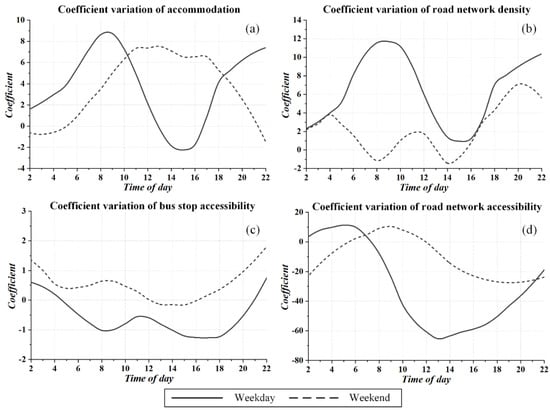
Figure 7.
Temporal variation of coefficients has different trends on weekdays and weekends.
The accessibility of the built environment also plays different roles in the temporal field of two daily types (Figure 7). In Manhattan, bus stop accessibility has a small positive effect on reducing the demand for taxis, but it is different on weekends. Surprisingly, the accessibility of the road network is negatively associated with taxi ridership in the off-peak time of weekdays, which means the less the travel time, the fewer people would like to take taxis. Its influence decreases during peak periods on weekdays while increasing during peak periods on weekends. This is mostly due to the high value of the travel time requirement in commuting on weekdays, which broadly supports the work in the area linking time values and travel [].
A high degree of mixing land use functions has played a role in reducing taxi trips, as mentioned before, which leads to a shorter travel distance, while this effect is more significant in the rush hours (Figure 8). Furthermore, intensive and diverse land functions always result in high accessibility of public transit stops, thus people have a better opportunity to travel by other modes for less money. Interestingly, there is an opposite trend in the transport entropy in temporal variation: more transportation options play a role in increasing the demand for taxis during peak periods on weekdays.
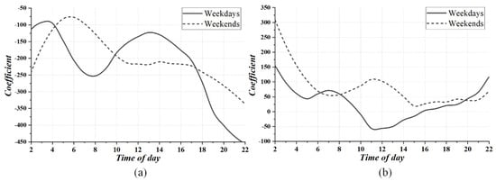
Figure 8.
Temporal variation of the estimated coefficients of entropy. (a) Land use entropy; (b) transport entropy.
5.4. Spatial Features
The active role of spatial distance is introduced in the regression process, leading to the variation in the spatial dimension of coefficients from GWR-based models. Visualization of spatial variation is possible by extracting the average value of the coefficients for a given time. Here, we focus on the analysis of the spatial variation throughout the day. Unlike previous studies that only discuss the impact of POIs density [], we highlight the spatial impact of diversity and accessibility on taxi ridership in this section.
5.4.1. Density of Railway Stations
Compared with other transport modes, increasing the density of railway stations is the most effective way to reduce the demand for taxis from the temporal perspective (Figure 6), but not all regions have similar characteristics. Here, we present the spatial variation of its average coefficients throughout the day (Figure 9). On the whole, the density of railway stations has a positive influence on increasing taxi demand in Brooklyn, northern Queens, and south-central Manhattan, and an average negative influence on Upper East Side, Upper West Side, and Upper Manhattan. The performance of the average coefficient when far away from the city center shows significant differences. In the areas surrounding John F. Kennedy International Airport, one of the hotspots in NYC [], the railway plays an important role in the reduction of taxis, while in the northeastern Queens with scarce railway stations, it does the opposite. It seems to be the result of a combination of passenger flow and railway accessibility for these districts; the subway plays a greater substitution role for cabs only when railways are highly accessible for numerous passengers.
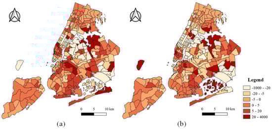
Figure 9.
Spatial variation of the average coefficients of the railway station density. (a) Weekdays; (b) weekends.
5.4.2. Entropy of POIs
Spatial variation of the average coefficients of entropy in land use function and travel modes are shown in Figure 10. The increased mix of land functions has a positive effect on reducing the number of taxi trips in most areas, particularly in Lower Manhattan, Midtown, and most areas of Upper Manhattan (Figure 10). On weekdays, a high mix of land uses at the Manhattan–Brooklyn border, in southern Brooklyn, and in northern Queens instead increases the number of taxi trips, and this pattern of impact diminishes or even disappears in several areas on weekends, which seems to be caused by the relatively fixed purpose and location of people commuting on weekdays. The degree of mixing of transportation shows the opposite effect on taxi ridership compared to the land use function (Figure 10). Specifically, in the areas around Midtown Manhattan and John F. Kennedy International Airport, the more transportation modes available, the greater the number of taxi rides. In contrast, in northern Queens and southern Bronx, more diverse transportation options reduce the number of taxi rides. We speculate that this is related to the accessibility of public transportation and the distance people travel. Remote areas have lower transit accessibility, people travel long distances and spend more on cabs (Figure 4), and setting a variety of developed travel modes can better compensate for this deficiency. In addition, the highly developed city center with various travel modes attracts more people from the outskirts, thus increasing the taxi ridership.
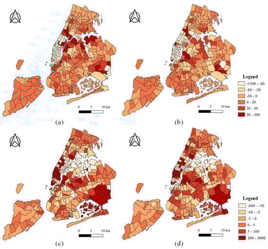
Figure 10.
Spatial variation of the average coefficients of entropy. (a,b) Land use entropy on weekdays and weekends. (c,d) Transport entropy on weekdays and weekends.
5.4.3. Accessibility of the Built Environment
The spatially averaged coefficients of accessibility from GTWR are shown in Figure 11. In most TAZs in Manhattan, high bus stop accessibility is effective in reducing the demand for taxis, and the same pattern of impact is seen in southern Queens. In contrast, in Brooklyn and Northeast Queens, high accessibility of bus stops promotes travel by taxi, which reflects the importance of taxis in long-distance travel []. The spatial heterogeneity of the road network accessibility coefficients is even more significant, with a low-accessibility network implying more passengers with long travel times for people to travel from the region (Figure 11). In Midtown Manhattan, Upper West Side, and Upper East Side, higher accessibility with less travel time significantly reduces the willingness of people to travel by taxi. In Lower Manhattan, Northern Brooklyn, and some remote areas, less congested road networks or short travel times encourage taxi ridership. It reflects the importance of travel time and expense when traveling medium to long distances by taxi.
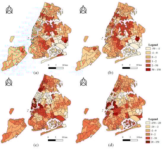
Figure 11.
Spatial variation of the average coefficients of accessibility. (a,b) Bus stop accessibility on weekdays and weekends. (c,d) Road network accessibility on weekdays and weekends.
6. Conclusions and Policy Implications
This study modeled the spatiotemporal heterogeneity of travel demand through GTWR, which outperforms OLS, GWR, and TWR in both goodness of fit and explanatory accuracy. Besides the analysis of travel patterns, this study developed an analytical framework to reveal the built environment’s influence on taxi ridership through multisource data in terms of density, design, diversity, and destination accessibility, and drew enlightening insights from temporal and spatial perspectives. The main findings of this study are summarized as follows:
- (1)
- People travel time and distance by taxi become longer the farther the origin TAZs are from the downtown. On weekdays, the average travel distance is 0.13 miles shorter than on weekends, but the average travel time is 2.3 min longer. For transit modes, there is a positive correlation between the railway and taxi ridership on weekdays, whereas it is negative on weekends. Buses have little impact on taxi ridership over the week. Moreover, bicycles have some role in reducing the taxi ridership.
- (2)
- In the downtown areas of the city, the density of public facilities, educational institutions, tourist facilities, and parking sites is positively associated with the demand for taxis, while health institutions and railway stations are negatively associated with it most of the time. The high density of accommodation and trunk road network increase taxi demand only during the daily peak period, while high bus stop accessibility and road network accessibility reduce taxi trips during the peak time.
- (3)
- Land use entropy significantly affects the travel behavior, with the highly mixed function reducing taxi ridership. However, highly mixed transportation hardly works in it. A highly mixed degree of transportation can only reduce taxi ridership in remote areas with underdeveloped public transportation, while in downtown areas it increases the taxi ridership.
- (4)
- Low-accessibility road network increases off-peak and evening peak taxi ridership and reduces it during the morning peak period, indicating that people think highly of travel time during weekday morning rush hours. In addition, in areas prone to congestion or longer travel times, low-accessibility road networks are more likely to reduce the demand for taxi trips. On average, the accessibility of the road network has a negative correlation with taxi ridership.
The results of this study have important implications for revealing the spatiotemporal characteristics of people’s dependence on taxis, improving the regulation of taxi operations, and balancing the distribution of urban transportation modes. The policy implications of this study are as follows.
- (1)
- At the present stage, most taxis prefer to carry passengers in central Manhattan, resulting in an uneven taxi distribution within the city. Our study found that a highly accessible road network increases people’s willingness to take taxis in the outer parts of the downtown, while in most parts of the central downtown, a highly accessible road network always results in a lower taxi travel demand. Taxi companies can take advantage of this feature to increase taxi deployment to parts of the downtown periphery during off-peak hours, and it is possible to increase the revenue of the taxi companies while maintaining a balance between the supply and demand of taxis between different urban districts.
- (2)
- As far as we know, in areas with well-developed transportation, travel time by subway is similar to and less costly than that offered by taxi. However, our study shows that in downtown areas, taxis are more irreplaceable in the morning peak hours than in the evening peak hours and on weekends, meaning that people prefer to spend more on transportation to ensure an efficient commute. Therefore, if the transfer between residential areas and railway stations is more convenient, people may reduce their reliance on taxis in the morning peak hours, which will also have a positive effect on alleviating the traffic congestion. As a result, the government can improve this situation by equipping convenient transfer services, such as developing MaaS (Mobility as a Service), improving the transfer infrastructure between shared bicycles and railway stations, or providing well-equipped park-and-ride facilities around the stations [].
- (3)
- Contrary to our perception, in general, offering a variety of transportation options has had little to no effect on reducing the taxi ridership, but has largely increased it, especially in downtown areas. However, larger variety of transit options may be effective in reducing taxi ridership in some remote areas where people travel for longer distances and at higher costs. The government could lighten the travel burden for residents by equipping them with convenient facilities of diverse transit modes in these districts. In addition, we believe that the essence of the solution to this problem lies in developing these remote areas with diverse land functions, which can fundamentally reduce the people’s travel time and travel distance and at the same time reduce the taxi influx to the downtown from these areas.
- (4)
- As analyzed in this paper, the positive correlation between the density of POIs for people’s spatiotemporal travel and taxi ridership is roughly consistent, such as people commuting between their workplace and residence on weekdays and mainly engaging in leisure and recreational activities on weekends, which increase the taxi ridership at some specific time of the day. Therefore, these relevant spatiotemporal hotspots can be equipped with convenient, esthetically pleasing, and orderly cabstands to enhance people’s travel experience during peak periods.
Based on multisource data, GTWR performs well in predicting and revealing the correlation characteristics of the built environment and taxi ridership from the spatiotemporal perspective. In the modeling process, the weight matrix of GTWR is characterized by the kernel function consisting of Euclidean distance and fixed bandwidth. However, travel behavior is a reflection of human activity carried by road networks, and whether the Euclidean distance metric is the most applicable for modeling by GTWR in transport analysis needs further discussion [,]. In addition, fixed bandwidth can be considered the ‘average value’ of the optimal bandwidth of multiple explanatory variables [], which makes the variables vary on the same scale between different analytical units. As a result, multiscale spatial variation can be achieved in the future by optimizing the bandwidth for each explanatory variable individually [,]. In this study, only one week of data in June was employed. The model can be developed in the future to explore the spatial and temporal travel demand characteristics in comparison to different seasons for a longer period.
Author Contributions
Conceptualization, C.X. and D.Y.; methodology, C.X.; software, C.X. and C.L.; validation, C.X., D.Y. and C.L.; formal analysis, C.X.; investigation, C.L.; resources, C.L.; data curation, B.P.; writing—original draft preparation, C.X.; writing—review and editing, C.X. and C.L.; visualization, C.X. and X.Z.; supervision, X.Z. and B.P.; project administration, D.Y.; funding acquisition, D.Y. All authors have read and agreed to the published version of the manuscript.
Funding
This research was funded by the Jilin Province Industrial Innovation Special Fund, grant No. 2019C024, and the Graduate Innovation Fund of Jilin University, grant No. 101832020CX149.
Institutional Review Board Statement
Not applicable.
Informed Consent Statement
Not applicable.
Data Availability Statement
The taxi record datasets are available from the public dataset of the New York City Taxi and Limousine Commission (TLC) at https://www1.nyc.gov/site/tlc/about/tlc-trip-record-data.page. (accessed on 10 May 2021).
Acknowledgments
The authors appreciate the reviewers and the editor for their insightful comments and suggestions.
Conflicts of Interest
The authors declare no conflict of interest.
Appendix A
Table A1.
Coefficient estimates on weekdays.
Table A1.
Coefficient estimates on weekdays.
| Explanatory Variable | MIN | LQ | MED | UQ | MAX |
|---|---|---|---|---|---|
| Public | −4700.84 | −1.94 | 0.00 | 3.54 | 13,254.00 |
| Leisure | −11,957.69 | −2.81 | 0.14 | 3.40 | 25,248.38 |
| Shopping | −15,614.50 | −0.72 | −0.01 | 0.57 | 608.00 |
| Tourism | −27,648.00 | −1.48 | 0.16 | 3.46 | 33,195.50 |
| Education | −6912.00 | −2.28 | −0.10 | 3.56 | 1439.14 |
| Health | −6912.00 | −2.05 | 0.08 | 3.05 | 224,952.00 |
| Accommodation | −55,029.00 | −5.00 | 0.00 | 5.25 | 19,514.00 |
| Worship | −5280.00 | −2.03 | 0.00 | 2.91 | 9131.75 |
| Taxi | −1,013,776.00 | −25.89 | 2.78 | 38.40 | 3,223,703.00 |
| Bus | −359.31 | −0.72 | 0.02 | 0.75 | 1316.54 |
| Railway | −5187.00 | −8.70 | −0.20 | 5.02 | 77,434.50 |
| Parking | −308,660.00 | −4.71 | 0.54 | 12.45 | 22,072.74 |
| Bicycle | −54282.00 | −0.47 | 0.07 | 0.94 | 4960.00 |
| Other | −585,032.00 | −57.39 | −2.56 | 12.65 | 705,660.00 |
| Trunk road network density | −111.43 | −2.54 | 0.00 | 1.91 | 5621.38 |
| Railway network density | −24,027.75 | −7.97 | 0.58 | 10.22 | 68,537.00 |
| Traffic signal density | −904.00 | −0.25 | 0.05 | 0.90 | 1585.41 |
| Land use entropy | −27,777.13 | −25.00 | −0.64 | 5.70 | 759.26 |
| Transport entropy | −19,684.75 | −15.50 | 0.10 | 25.79 | 22,070.00 |
| Bus stop accessibility | −6042.88 | −0.32 | 0.15 | 0.92 | 5170.72 |
| Road network accessibility | −793.29 | −4.80 | 0.00 | 2.66 | 450.56 |
Table A2.
Coefficient estimates on weekends.
Table A2.
Coefficient estimates on weekends.
| Explanatory Variable | MIN | LQ | MED | UQ | MAX |
|---|---|---|---|---|---|
| Public | −2461.65 | −2.47 | 0.00 | 2.94 | 1956.94 |
| Leisure | −1059.13 | −2.27 | 0.41 | 4.89 | 1752.94 |
| Shopping | −1964.19 | −0.88 | −0.04 | 0.59 | 2555.51 |
| Tourism | −23,282.25 | −1.63 | 0.26 | 2.80 | 18,818.95 |
| Education | −1176.50 | −2.76 | −0.08 | 3.39 | 3006.29 |
| Health | −9643.46 | −2.53 | 0.00 | 2.35 | 6328.18 |
| Accommodation | −8453.22 | −5.89 | 0.00 | 5.36 | 7023.74 |
| Worship | −1472.50 | −1.57 | 0.09 | 4.01 | 2253.11 |
| Taxi | −8,597,000.00 | −16.00 | 8.00 | 48.00 | 9,123,000.00 |
| Bus | −167.66 | −0.72 | 0.02 | 1.07 | 262.34 |
| Railway | −12,697.70 | −12.83 | −0.91 | 3.44 | 1599.92 |
| Parking | −10,323.40 | −6.10 | 0.08 | 9.64 | 32,130.99 |
| Bicycle | −1784.69 | −0.47 | 0.10 | 0.98 | 1579.45 |
| Other | −704,512.00 | −70.90 | −3.40 | 14.50 | 174,186.00 |
| Trunk road network density | −441.35 | −3.46 | −0.05 | 1.10 | 313.19 |
| Railway network density | −2963.90 | −6.88 | 0.46 | 12.91 | 10,454.38 |
| Traffic signal density | −271.84 | −0.26 | 0.06 | 0.82 | 177.75 |
| Land use entropy | −2357.49 | −38.69 | −1.81 | 3.49 | 665.80 |
| Transport entropy | −993.82 | −9.05 | 1.00 | 34.33 | 12,449.50 |
| Bus stop accessibility | −789.97 | −0.20 | 0.23 | 1.48 | 731.02 |
| Road network accessibility | −3953.55 | −3.56 | −0.04 | 0.96 | 4009.29 |
Table A3.
Comparisons of average coefficients in different peak times.
Table A3.
Comparisons of average coefficients in different peak times.
| Explanatory Variable | Weekdays | Weekends | ||
|---|---|---|---|---|
| Morning Peak (7 am–10 am) | Evening Peak (5 pm–8 pm) | Noon Peak (12 pm–3 pm) | Evening Peak (5 pm–8 pm) | |
| Public | −3.23 | −4.63 | −1.72 | 6.02 |
| Leisure | −5.89 | 31.66 | 0.94 | 0.81 |
| Shopping | 0.37 | −7.75 | −1.24 | 5.46 |
| Tourism | −4.41 | 55.07 | 5.00 | 28.82 |
| Education | 1.62 | 0.43 | −1.50 | 10.91 |
| Health | −1.94 | 10.95 | 1.05 | −30.40 |
| Accommodation | 2.48 | 23.01 | 5.64 | 21.10 |
| Worship | −2.43 | 7.14 | 2.88 | −5.11 |
| Taxi | 282.71 | −66.80 | 31.41 | −108.54 |
| Bus | −0.77 | 0.94 | 0.27 | 0.74 |
| Railway | −2.04 | 0.10 | −1.71 | −38.97 |
| Parking | 7.34 | −16.01 | −16.66 | −7.44 |
| Bicycle | 0.91 | −15.62 | −0.86 | −2.46 |
| Other | −20.26 | 1037.86 | 20.28 | 332.58 |
| Trunk road network density | 2.02 | 1.33 | −2.31 | −4.11 |
| Railway network density | 4.75 | −42.14 | −5.97 | 16.82 |
| Traffic signal density | 0.50 | 2.96 | 0.92 | 0.18 |
| Land use entropy | −60.90 | −95.37 | −56.08 | −74.33 |
| Transport entropy | 1.76 | 39.92 | 24.41 | 57.01 |
| Bus stop accessibility | 0.37 | 4.86 | 1.17 | −0.62 |
| Road network accessibility | 1.71 | −9.19 | −0.96 | −14.79 |
References
- Ma, X.; Zhang, J.; Ding, C.; Wang, Y. A Geographically and Temporally Weighted Regression Model to Explore the Spatiotemporal Influence of Built Environment on Transit Ridership. Comput. Environ. Urban Syst. 2018, 70, 113–124. [Google Scholar] [CrossRef]
- Shen, X.; Zhou, Y.; Jin, S.; Wang, D. Spatiotemporal Influence of Land Use and Household Properties on Automobile Travel Demand. Transp. Res. Part D Transp. Environ. 2020, 84, 102359. [Google Scholar] [CrossRef]
- Qian, X.; Ukkusuri, S.V. Spatial Variation of the Urban Taxi Ridership Using GPS Data. Appl. Geogr. 2015, 59, 31–42. [Google Scholar] [CrossRef]
- Tang, J.; Gao, F.; Liu, F.; Zhang, W.; Qi, Y. Understanding Spatio-Temporal Characteristics of Urban Travel Demand Based on the Combination of GWR and GLM. Sustainability 2019, 11, 5525. [Google Scholar] [CrossRef] [Green Version]
- Chen, C.; Feng, T.; Ding, C.; Yu, B.; Yao, B. Examining the Spatial-Temporal Relationship between Urban Built Environment and Taxi Ridership: Results of a Semi-Parametric GWPR Model. J. Transp. Geogr. 2021, 96, 103172. [Google Scholar] [CrossRef]
- Liu, Q.; Ding, C.; Chen, P. A Panel Analysis of the Effect of the Urban Environment on the Spatiotemporal Pattern of Taxi Demand. Travel Behav. Soc. 2020, 18, 29–36. [Google Scholar] [CrossRef]
- Hochmair, H.H. Spatiotemporal Pattern Analysis of Taxi Trips in New York City. Transp. Res. Rec. 2016, 2542, 45–56. [Google Scholar] [CrossRef]
- Tang, J.; Zhu, Y.; Huang, Y.; Peng, Z.-R.; Wang, Z. Identification and Interpretation of Spatial–Temporal Mismatch between Taxi Demand and Supply Using Global Positioning System Data. J. Intell. Transp. Syst. 2019, 23, 403–415. [Google Scholar] [CrossRef]
- Ni, Y.; Chen, J. Exploring the Effects of the Built Environment on Two Transfer Modes for Metros: Dockless Bike Sharing and Taxis. Sustainability 2020, 12, 2034. [Google Scholar] [CrossRef] [Green Version]
- Ewing, R. Is Los Angeles-Style Sprawl Desirable? J. Am. Plan. Assoc. 1997, 63, 107–126. [Google Scholar] [CrossRef]
- Ewing, R.; Tian, G.; Lyons, T. Does Compact Development Increase or Reduce Traffic Congestion? Cities 2018, 72, 94–101. [Google Scholar] [CrossRef] [Green Version]
- Horváth, M.T.; Mátrai, T.; Tóth, J. Route Planning Methodology with Four-Step Model and Dynamic Assignments. Transp. Res. Procedia 2017, 27, 1017–1025. [Google Scholar] [CrossRef]
- Chen, E.; Ye, Z.; Wang, C.; Zhang, W. Discovering the Spatio-Temporal Impacts of Built Environment on Metro Ridership Using Smart Card Data. Cities 2019, 95, 102359. [Google Scholar] [CrossRef]
- Ewing, R.; Cervero, R. Travel and the Built Environment: A Meta-Analysis. J. Am. Plan. Assoc. 2010, 76, 265–294. [Google Scholar] [CrossRef]
- Egu, O.; Bonnel, P. How Comparable Are Origin-Destination Matrices Estimated from Automatic Fare Collection, Origin-Destination Surveys and Household Travel Survey? An Empirical Investigation in Lyon. Transp. Res. Part A Policy Pract. 2020, 138, 267–282. [Google Scholar] [CrossRef]
- Bian, R.; Wilmot, C.G.; Wang, L. Estimating Spatio-Temporal Variations of Taxi Ridership Caused by Hurricanes Irene and Sandy: A Case Study of New York City. Transp. Res. Part D Transp. Environ. 2019, 77, 627–638. [Google Scholar] [CrossRef]
- Tracy, A.J.; Su, P.; Sadek, A.W.; Wang, Q. Assessing the Impact of the Built Environment on Travel Behavior: A Case Study of Buffalo, New York. Transportation 2011, 38, 663–678. [Google Scholar] [CrossRef]
- Ma, X.; Ji, Y.; Yuan, Y.; Van Oort, N.; Jin, Y.; Hoogendoorn, S. A Comparison in Travel Patterns and Determinants of User Demand between Docked and Dockless Bike-Sharing Systems Using Multisourced Data. Transp. Res. Part A Policy Pract. 2020, 139, 148–173. [Google Scholar] [CrossRef]
- Yu, H.; Peng, Z.-R. The Impacts of Built Environment on Ridesourcing Demand: A Neighbourhood Level Analysis in Austin, Texas. Urban Stud. 2020, 57, 152–175. [Google Scholar] [CrossRef]
- De Abreu e Silva, J.; Morency, C.; Goulias, K.G. Using Structural Equations Modeling to Unravel the Influence of Land Use Patterns on Travel Behavior of Workers in Montreal. Transp. Res. Part A Policy Pract. 2012, 46, 1252–1264. [Google Scholar] [CrossRef]
- Yu, L.; Xie, B.; Chan, E. How Does the Built Environment Influence Public Transit Choice in Urban Villages in China? Sustainability 2018, 11, 148. [Google Scholar] [CrossRef] [Green Version]
- Sabouri, S.; Park, K.; Smith, A.; Tian, G.; Ewing, R. Exploring the Influence of Built Environment on Uber Demand. Transp. Res. Part D Transp. Environ. 2020, 81, 102296. [Google Scholar] [CrossRef]
- Huang, G.; Qiao, S.; Yeh, A.G.-O. Spatiotemporally Heterogeneous Willingness to Ridesplitting and Its Relationship with the Built Environment: A Case Study in Chengdu, China. Transp. Res. Part C Emerg. Technol. 2021, 133, 103425. [Google Scholar] [CrossRef]
- Hawkins, J.; Nurul Habib, K. Travel Distance and Land Use: A Generalized Box–Cox Model with Conditional Spatial Lag Dependence. Transp. A Transp. Sci. 2021, 17, 1101–1121. [Google Scholar] [CrossRef]
- Wang, S.; Yu, D.; Ma, X.; Xing, X. Analyzing Urban Traffic Demand Distribution and the Correlation between Traffic Flow and the Built Environment Based on Detector Data and POIs. Eur. Transp. Res. Rev. 2018, 10, 50. [Google Scholar] [CrossRef]
- Yu, H.; Peng, Z.-R. Exploring the Spatial Variation of Ridesourcing Demand and Its Relationship to Built Environment and Socioeconomic Factors with the Geographically Weighted Poisson Regression. J. Transp. Geogr. 2019, 75, 147–163. [Google Scholar] [CrossRef]
- Huang, B.; Wu, B.; Barry, M. Geographically and Temporally Weighted Regression for Modeling Spatio-Temporal Variation in House Prices. Int. J. Geogr. Inf. Sci. 2010, 24, 383–401. [Google Scholar] [CrossRef]
- GaWC. The World According to GaWC 2020; GaWC: Leicestershire, UK, 2020. [Google Scholar]
- Shannon, C.; Weaver, W. The Mathematical Theory of Communication; The University of Illinois Press: Champaign, IL, USA, 1964; 131p. [Google Scholar]
- Zeng, S.; Yang, P.; Fang, D. Accessibility Assessment on Structure of Street Network. J. Tongji Univ. Nat. Sci. Ed. 2001, 29, 666–672. [Google Scholar]
- Wu, H.; Levinson, D. Unifying Access. Transp. Res. Part D Transp. Environ. 2020, 83, 102355. [Google Scholar] [CrossRef]
- Hansen, W.G. How Accessibility Shapes Land Use. J. Am. Inst. Plan. 1959, 25, 73–76. [Google Scholar] [CrossRef]
- El-Geneidy, A.; Grimsrud, M.; Wasfi, R.; Tétreault, P.; Surprenant-Legault, J. New Evidence on Walking Distances to Transit Stops: Identifying Redundancies and Gaps Using Variable Service Areas. Transportation 2014, 41, 193–210. [Google Scholar] [CrossRef]
- Gutiérrez, J.; García-Palomares, J.C. Distance-Measure Impacts on the Calculation of Transport Service Areas Using GIS. Environ. Plan. B Plan. Des. 2008, 35, 480–503. [Google Scholar] [CrossRef]
- Fotheringham, A.S.; Brunsdon, C.; Charlton, M. Geographically Weighted Regression: The Analysis of Spatially Varying Relationships; John Wiley & Sons: Hoboken, NJ, USA, 2002; ISBN 978-0-471-49616-8. [Google Scholar]
- Fotheringham, A.S.; Crespo, R.; Yao, J. Geographical and Temporal Weighted Regression (GTWR): Geographical and Temporal Weighted Regression. Geogr. Anal. 2015, 47, 431–452. [Google Scholar] [CrossRef] [Green Version]
- Lei, F. Travel Intensity Influencing Factors Analysis Model Based on Signaling Data. J. Transp. Syst. Eng. Inf. Technol. 2020, 20, 51–55. [Google Scholar]
- Brunsdon, C.; Fotheringham, A.S.; Charlton, M.E. Geographically Weighted Regression: A Method for Exploring Spatial Nonstationarity. Geogr. Anal. 2010, 28, 281–298. [Google Scholar] [CrossRef]
- Gollini, I.; Lu, B.; Charlton, M.; Brunsdon, C.; Harris, P. GWmodel: An R Package for Exploring Spatial Heterogeneity Using Geographically Weighted Models. J. Stat. Soft. 2015, 63, 1–50. [Google Scholar] [CrossRef] [Green Version]
- Lu, B.; Harris, P.; Charlton, M.; Brunsdon, C. The GWmodel R Package: Further Topics for Exploring Spatial Heterogeneity Using Geographically Weighted Models. Geo-Spat. Inf. Sci. 2014, 17, 85–101. [Google Scholar] [CrossRef]
- Li, Y.; Xiong, W.; Wang, X. Does Polycentric and Compact Development Alleviate Urban Traffic Congestion? A Case Study of 98 Chinese Cities. Cities 2019, 88, 100–111. [Google Scholar] [CrossRef]
- Xie, C.; Yu, D.; Zheng, X.; Wang, Z.; Jiang, Z. Revealing Spatiotemporal Travel Demand and Community Structure Characteristics with Taxi Trip Data: A Case Study of New York City. PLoS ONE 2021, 16, e0259694. [Google Scholar] [CrossRef]
- Ulak, M.B.; Yazici, A.; Aljarrah, M. Value of Convenience for Taxi Trips in New York City. Transp. Res. Part A Policy Pract. 2020, 142, 85–100. [Google Scholar] [CrossRef]
- Zhang, X.; Xu, Y.; Tu, W.; Ratti, C. Do Different Datasets Tell the Same Story about Urban Mobility—A Comparative Study of Public Transit and Taxi Usage. J. Transp. Geogr. 2018, 70, 78–90. [Google Scholar] [CrossRef]
- Zheng, L.; Xie, Z.; Ding, T.; Xi, J.; Meng, F. Parking and Ride Induction Methods for Drivers in Commuting Scenes. Symmetry 2021, 13, 2176. [Google Scholar] [CrossRef]
- Lu, B.; Charlton, M.; Harris, P.; Fotheringham, A.S. Geographically Weighted Regression with a Non-Euclidean Distance Metric: A Case Study Using Hedonic House Price Data. Int. J. Geogr. Inf. Sci. 2014, 28, 660–681. [Google Scholar] [CrossRef]
- Lu, B.; Brunsdon, C.; Charlton, M.; Harris, P. Geographically Weighted Regression with Parameter-Specific Distance Metrics. Int. J. Geogr. Inf. Sci. 2017, 31, 982–998. [Google Scholar] [CrossRef] [Green Version]
- Yu, H.; Fotheringham, A.S.; Li, Z.; Oshan, T.; Kang, W.; Wolf, L.J. Inference in Multiscale Geographically Weighted Regression. Geogr. Anal. 2020, 52, 87–106. [Google Scholar] [CrossRef]
- Fotheringham, A.S.; Yang, W.; Kang, W. Multiscale Geographically Weighted Regression (MGWR). Ann. Am. Assoc. Geogr. 2017, 107, 1247–1265. [Google Scholar] [CrossRef]
- Wu, C.; Ren, F.; Hu, W.; Du, Q. Multiscale Geographically and Temporally Weighted Regression: Exploring the Spatiotemporal Determinants of Housing Prices. Int. J. Geogr. Inf. Sci. 2019, 33, 489–511. [Google Scholar] [CrossRef]
Publisher’s Note: MDPI stays neutral with regard to jurisdictional claims in published maps and institutional affiliations. |
© 2022 by the authors. Licensee MDPI, Basel, Switzerland. This article is an open access article distributed under the terms and conditions of the Creative Commons Attribution (CC BY) license (https://creativecommons.org/licenses/by/4.0/).