Abstract
Investigation shows that train travel has a lower pollution impact on the environment than flight travel or car travel. A stated preferences (SP) survey can effectively obtain the data of the commuter’s response to the hypothetical train price changes beyond the scope of previous observations. To this end, based on SP survey, we estimate the price elasticity of train travel demand and analyze its variation rules. It is shown that: (1) the own-price elasticities of demand are −1.049028 during peak period and −1.090438 during off-peak period, respectively; (2) the cross-price elasticities of demand are 0.001280 for train and air and 0.001156 for train and car during peak period; and 0.001350 for train and air and 0.001230 for train and car during off-peak period; (3) the own and cross-price elasticities of demand during off-peak period are bigger than the ones during peak period; (4) when the influence factors’ influence degree is 3 or 5, the own and cross-price elasticities of demand are largest; when the influence degree is 1, the own and cross-price elasticities of demand are smallest. A result application example shows that the elasticities obtained from this paper could be used to reduce energy used and CO2 emissions effectively.
1. Introduction
Train travel is a common means of travel, and as one of the main intercity travel modes, railway bears a large amount of passenger flow. Train travel helps protect the environment by reducing energy consumption and the release of pollutants such as CO2 into the atmosphere. Table 1 [1] shows that intercity railways use less energy than planes, cars or buses, and generally emit less carbon dioxide than planes or cars.

Table 1.
Energy used and CO2 emissions of the main travel modes [1].
A passenger kilometer means one passenger traveling one kilometer.
Train travel is an important way to reduce energy used and air pollution emissions. Train fare is an important economic lever to adjust train travel, which affects travelers’ travel behavior and choice of travel mode. The price elasticity of train travel demand is a key determinant of investigating many related issues, such as the effects of train fare changes or train system development and expansion [1,2]. Therefore, the study of the price elasticity of train travel demand has important theoretical and practical significance. Combining with the related literature and based on a stated preferences (SP) survey, this paper estimates the train travel demand own-and cross-price elasticities, and analyzes variation rules of the train travel demand price elasticities with the change in traveler attributes and influence factors’ influence degree, and then uses a result application example to show how the elasticities of this paper can be used to reduce the energy used and CO2 emissions effectively, which also partly shows the reliability and validity of the price elasticity of demand of this paper. The results of this paper can provide some scientific basis for the correct formulation of train fares and reducing energy consumption and CO2 emissions.
There are several main contributions of this paper: (1) the own-price elasticities of demand for train travel and the cross-price elasticities of demand for train and air, and train and car, are estimated; (2) their variation rules with the change in traveler attributes and influence factors influence degree are analyzed; (3) a result application example shows that the elasticities of this paper could be used to reduce energy used and CO2 emissions effectively.
The remainder of this paper is organized as follows. Section 2 reviews some relevant research. Section 3 describes the data. Section 4 presents the methodology used to estimate the own-and cross-price elasticities of train travel demand. Section 5 presents the own- and cross-price elasticity results and their variation rules and application to reduce energy used and CO2 emissions, and carries out the further discussion. Finally, the conclusions of the paper are given in Section 6.
2. Relevant Literature Review
Investigation on the price elasticity of demand for various travel modes has become a research hotspot. Many scholars have studied the price elasticity of demand for various travel modes based on the actual data and model methods, such as the price elasticity of demand of public transport travel [2,3,4,5,6,7,8,9], including the price elasticity of demand of subway travel [5,6,7,8,9], and the price elasticity of demand of air travel [1,10,11].
Some scholars investigated the price elasticity of train travel demand. Based on SP survey and the nested logit model, Anciaes et al. [12] studied the influence of the complex structure of railway fares on train travel demand, and found that simplifying the structure of fares would not increase rail travel demand. Wardman [13] conducted the largest price elasticity analysis of travel demand based on meta-analysis, covering 167 studies in the UK and 1633 studies on the elasticities of surface traffic patterns such as cars, railways, buses and subways. In order to assess whether travelers would switch from plane to train and use the new rail systems, Gama [1] used the method described in Berry [14] to estimate domestic flights’ and passenger trains’ own- and cross-price elasticities of demand; the static model of this study showed that there was little substitutability between these two modes of transportation. Combining with the train fare reduced by 20% in Sydney in 1976, Hensher and Bullock [15] examined the misreading effects of the actual price changes and the role of other factors other than cost to determine the effects of the reducing price on the real demand for travel. Nowak and Savage [16] calculated the cross-price elasticities between gasoline prices and ridership volume in Chicago based on monthly data from January 1999 to 2010, and estimated rail, city bus, commuter rail and suburban bus services, respectively. Ignacio [17] studied the price elasticity of demand and income elasticity of various intercity travel modes in the Northwest Corridor of the United States, and reconstructed the travel volume data and price data. Li et al. [18] used a revealed preferences (RP) survey to study the freight demand price elasticity of different travel modes such as railway in five countries.
The stated preferences (SP) survey can effectively obtain data that cannot be directly obtained by revealed preferences (RP) survey or observation and is used in many aspects of traffic research to reveal respondent’s presumed behavior in hypothetical situations, such as [12,19,20,21,22]. Based on an SP survey, Sipes and Mendelsohn [19] asked how many miles drivers would drive in response to the gasoline price increase and found that drivers would change their driving behavior in response to the higher gasoline prices, and drivers were price inelastic, and the income elasticity of gasoline was also low. Hössinger et al. [20] used the stated preferences (SP) survey derived from scenario analysis to estimate the price elasticity of fuel demand. Research showed that the application of the situational stated preferences (SP) survey was particularly useful if environments were not sufficiently stable, namely, the forecast period differs from the data period used for elasticity estimation, such as the travelers’ response to the hypothetical train price changes beyond the scope of previous observations.
Some typical factors affecting the price elasticity of train travel demand are as follows [2,8,23,24]:
(1) Departure frequency. The departure frequency is related to the waiting time of travelers. When the departure frequency is low, travelers may have more chances to choose other travel modes, which makes it easy to lose passenger flow and affects the attraction of train travel. At this time, when the train fare increases, travelers are more sensitive to the train price, and vice versa;
(2) Travel time. With the popularization of faster travel modes such as the air, the length of travel time has become one of the most important factors to be considered when choosing train travel. When the train travel time is generally too long, travelers’ demand for choosing train travel reduces. At this time, when the train fare increases, travelers are more sensitive to the train price, and vice versa;
(3) Service level. As people’s quality of life improves, people have more and more high-quality transportation service requests such as comfort and convenience, which mainly include punctuality, the in-vehicle environment and congestion, and transfer convenience, and the connectivity with other modes of transport. Additionally, the commuters will choose the travel mode which has high punctuality, and whose in-vehicle environment is better and in-vehicle congestion is less than other travel modes, which can easily transfer to other modes of transport, such as taxis and buses and so on. When train travel service level is high, when train fare increases, travelers are less sensitive to the train price, and vice versa;
(4) Travel purpose. The price elasticity of demand varies with different travel purposes. For example, the demand for official and business travel is characterized by relatively stable demand and higher requirements for travel time and the traveler’s travel expenses belong to product or labor costs, and therefore the traveler is less sensitive to the train fare. For personal affairs and travel purposes, the train is preferred as a cheap and slow travel mode compared with planes, and the traveler’s travel expenses belong to personal income, and therefore the traveler is more sensitive to the train fare;
(5) Relevant travel mode’s price. The relevant travel mode’s price affects the price elasticity of train travel demand. For example, when the price of air decreases, the demand for air travel increases, and then the demand for train travel decreases accordingly. When the train price increases, travelers are more sensitive to the train price; when the train price reduces, travelers are less sensitive to the train price;
(6) Level of urbanization. Urban people’s income level is generally higher than that of rural areas, and travel spending in daily life is also higher; the travel rate of urban areas is much higher than the one for rural areas. The rhythm for urban working is faster, and therefore people need a short travel time to enjoy, and rest and loosen their body and mind by changing their daily life environment, so the travel demand of the city is stronger than the one of the rural area, and in a higher level of urbanization, travelers are less sensitive to the train price, and vice versa.
In addition, some scholars investigated the application of various price elasticities in energy used and CO2 emissions, such as the price and income elasticities of oil demand [25,26], the time-varying income and price elasticities for energy demand [27], the price and income elasticities for coal demand [28] and the fuel demand price elasticities [29].
3. Data
The stated preferences (SP) survey is particularly suited to discrete choice experiments and is usually employed to reveal respondent’s presumed transportation behavior in hypothetical situations [20]. For more detailed description and mechanisms of the SP survey, see [12,19,20,21,22]. This paper uses an online survey to collect data based on the SP survey. According to the purpose of the paper, the structure of the questionnaire is divided into three parts: the survey of personal attributes of travelers, the survey of the own- and cross-price elasticities of train travel demand, and the survey of influence factors’ influence degree on train travel demand price elasticity, which are as follows:
- (1)
- Survey of personal attributes of travelers
A survey of personal attributes of travelers is used to acquire the properties of respondents, including gender, age, education background, occupation background, travel distance for long-distance travel (cross-province, cross-city), proportion of travelers’ long-distance travel (cross-province, cross-city) by train, monthly income level, etc., and the problem and its option value settings are based on the related literature research and the real traffic;
- (2)
- Survey of the price elasticity of train travel demand
According to the research purpose of this paper, in this paper, based on an SP survey and the hypothetical train price changes beyond the scope of previous observations, we estimate the own-price elasticities of demand for train travel and the cross-price elasticities of demand for train and air, and train and car. More specifically, the problems are set as follows: when the train fares increase by 10%, 20%, 30% and 40%, respectively, how many percentages does your train travel reduce on the basis of the original and how many percentages do your relevant traffic modes travel increase on the basis of the original;
- (3)
- Survey of influence factors influence degree of train travel demand price elasticity
The content of this part of the questionnaire is arranged according to the content of the above influence factors’ analysis. The main purpose is to study the variation rules of own- and cross-price elasticities of demand with the change in influence factors’ influence degree. Considering that the influence factors’ influence degree cannot be accurately quantified, when setting the problem and value of this part, a 5-point Likert-type scale [30] is adopted, and the influence factors’ influence degree is divided into five grades: 1 means no influence, 2 means a little influence, 3 means general influence, 4 means big influence, and 5 means very big influence. Respondents were required to score the influence factors’ influence degree in the questionnaire on train travel according to their own past experiences and feelings and the above classification method.
Trains are mainly used for long-distance travel cross provinces and cities. From this perspective, the substitutable travel modes of train are mainly air and car. Thus, the questionnaire requires that the respondents have had train, plane and car travel experiences in the last 12 months. There is a big difference in the travel characteristics of peak period and off-peak periods, which may mean that train travel demand price elasticity is different, and therefore, in this questionnaire, to ensure the accuracy of the survey results, the investigation is divided into two types: peak period and off-peak period. To validate the questionnaire, some transportation planning and management professors were invited to assess whether the questionnaire was appropriate for estimating the price elasticity of train travel demand. According to the professors’ feedback, we modified the questionnaire. To test whether the survey instrument was well behaved and whether individuals understood the questionnaire items, a pre-test was conducted with 30 people. The questionnaire was also modified according to respondents’ feedback.
The questionnaire was written in Chinese and distributed online between 11 April 2020 and 19 April 2020, and most provinces and cities in China were covered. A total of 335 questionnaires were collected. Next, we extracted and checked the sample data. According to principles of effectiveness and consistently in the process of investigation, the questionnaires that could not be completed were eliminated. According to the time that the respondents took to fill out the questionnaire in the pre-test, we took 100 s as the minimum filling time of the questionnaire. In the online survey, if the filling time was less than 100 s, it would be eliminated. During the questionnaire survey, if there was a logical contradiction in the travel data provided by the respondents, the consistency principle was violated, and it was also eliminated. Finally, 35 were eliminated and the effective questionnaire volume obtained was 300, and the effective rate was 89.6%. The subsequent data analysis was based on the data of these 300 questionnaires. The characteristics of the samples were as follows: male respondents accounted for 51.3% and female respondents accounted for 48.7%. Most of the respondents were within the under-25 age range (32%) and 36–45 age range (31.3%). A total of 88.3% of respondents are undergraduates of university or above. In terms of occupation background, 30.3% of respondents were ordinary staff, 23.3% of respondents were the base manager, 20.7% of respondents were students, and 15% of respondents were the middle manager. In terms of travel distance for long-distance travel (cross-province, cross-city), 501–1000 km accounted for 31.7%, 100–500 km accounted for 20.7%, 1001–3000 km accounted for 19.3% and 3001–5000 km accounted for 14.7%. In terms of proportion of travelers’ long-distance travel (cross-province, cross-city) by train, the proportion range 10–30% accounted for 36%, the proportion range 31–50% accounted for 21%, the proportion range 51–70% accounted for 14.7%, and the proportion range more than 90% accounted for 11%. A total of 38.7% of respondents’ monthly income level was 8001–10,000 yuan, 29% of respondents’ monthly income level was less than 2000 yuan and 15.3% of respondents’ monthly income level was more than 10,000 yuan, where yuan is the monetary unit of China.
4. Methodology
The price elasticity of demand, which is adopted in this paper can be calculated as follows
where is the price elasticity of demand coefficient, represents the demand for goods and represents the price of goods, and represents the change in the demand for goods and represents the change in the price of goods. The price elasticity of demand coefficient reflects the sensitivity of demand to price change. Based on the collected data, the specific calculation processes and formulas in this paper are as follows:
(1) Combining with the data, Equation (1) is used to calculate the own-price elasticities of demand and the cross-price elasticities of demand of the traveler when the train fare changes by during peak period and off-peak period respectively, where represents peak period or off-peak period and represents air or car travel modes;
(2) Calculate the own-price elasticities of demand of the traveler during peak period and off-peak period
and the corresponding cross-price elasticities of demand
(3) Calculate the own-price elasticities of demand of travelers during peak period and off-peak period when train fare increases by
and the corresponding cross-price elasticities of demand
(4) Calculate the final own-price elasticities of demand for train travel during peak period and off-peak period
and the corresponding cross-price elasticities of demand
(5) The own and cross-price elasticities of demand for an attribute taking a certain value or an influence factor influence degree taking a certain value are calculated as the average value of the corresponding elasticities of the travelers, whose attribute takes the corresponding value or influence factor influence degree takes the corresponding value.
5. Results and Discussion
5.1. Own-Price Elasticities of Demand
According to the corresponding data and methods, the own-price elasticities of demand changing during peak period and off-peak period when the train price increases by are shown by Figure 1.
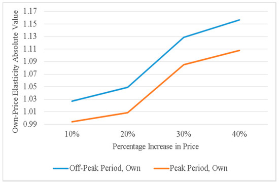
Figure 1.
Own-price elasticities of demand changing when train fare increases by
Figure 1 shows that when train fares increase by 10%, 20%, 30% and 40%, respectively, the own-price elasticities during peak period and off-peak period increase with the increase in train fare change, which is consistent with the real traffic, namely, with the increase in train fare change, travelers are more sensitive to the train price, and vice versa; Figure 1 also shows that own-price elasticities during the off-peak period are bigger than the ones during peak period, which may be because during peak period, there are more travelers choosing to travel by train, and therefore travelers are less sensitive to the train price, and vice versa; furthermore, when the train fare increases from 20% to 30%, own-price elasticities change greatly.
According to the corresponding data and calculation method, own-price elasticity we obtained during peak period is −1.049028, and that during off-peak period is −1.090438.
5.2. Cross-Price Elasticities of Demand
According to the corresponding data and methods, the cross-price elasticities of demand changing during peak period and off-peak period when the train price increases by are shown by Figure 2.
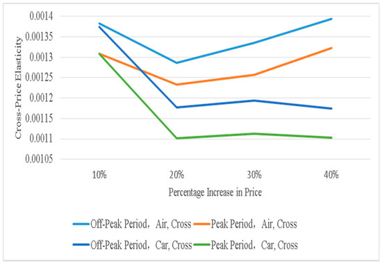
Figure 2.
Cross-price elasticities of demand changing when train fare increases by .
Figure 2 shows that overall, the cross-price elasticities of demand for train and air, and train and car, during off-peak period are bigger than the ones during peak period, respectively, which may be because during peak period, traffic flow is larger, and travelers have fewer chances to choose other travel modes. When the train fare increases from 10% to 20%, the cross-price elasticities of demand for train and air, and train and car, during peak period and off-peak period decrease. When the fare increases from 20% to 40%, the cross-price elasticities of demand for train and air during peak period and off-peak period show a rising trend, and the cross-price elasticities of demand for train and car during peak period and off-peak period show a trend of a slight increase and then a slight decrease.
According to the data and calculation method, the cross-price elasticities of demand we obtained during peak period are 0.001280 for train and air and 0.001156 for train and car; and the cross-price elasticities of demand during off-peak period are 0.001350 for train and air and 0.001230 for train and car.
5.3. Variation Rules of the Own- and Cross-Price Elasticities of Demand
Next, we investigate the variation rules of the own- and cross-price elasticities of demand with the change in traveler attributes and the influence factors’ influence degree.
5.3.1. Variation Rules with the Change in Traveler Attributes
Variation rules of the own and cross-price elasticities of demand with the change in traveler attributes during peak period and off-peak period are as follows. Figure 3 below shows the variation rules of the own- and cross-price elasticities of demand with the change in traveler’s gender attribute.
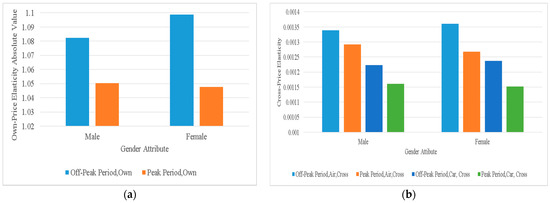
Figure 3.
The variation rules of the own- and cross-price elasticities of demand with the change in traveler’s gender attribute: (a) own-price elasticities of demand; (b) cross-price elasticities of demand.
Figure 3a shows that the own-price elasticities of female travelers have a bigger difference between peak period and off-peak period. During the off-peak period, female own-price elasticities are bigger than male own-price elasticities, while during peak period, male own-price elasticities are slightly bigger than female own-price elasticities. Figure 3b shows that when the gender is female, cross-price elasticities for train and air change more obviously during peak period and off-peak period. During peak period, there are more travelers choosing to travel by train and traffic flow is larger and travelers have fewer chances to choose other travel modes, so the own- and cross-price elasticities during off-peak period are larger than the ones during peak period.
Figure 4 shows the variation rules of the own- and cross-price elasticities of demand with the change in traveler’s age attribute.
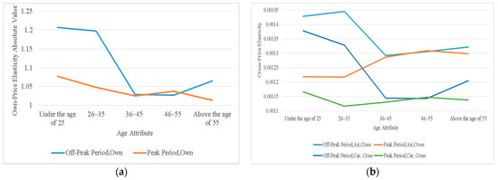
Figure 4.
The variation rules of the own and cross-price elasticities of demand with the change in traveler’s age attribute. (a) own-price elasticities of demand; (b) cross-price elasticities of demand.
Figure 4a shows when age is under 25, the own-price elasticities have maximum value, and in the 26~45 years old age range, the own-price elasticities diminishes with age, and the own-price elasticities during off-peak period are greater than the ones during peak period. After age 45, the own-price elasticities during peak period firstly increase and then decrease, and during off-peak period they firstly decrease and then increase. Figure 4b shows that when age is under 25, the cross-price elasticities during off-peak period are largest; the cross-price elasticities for train and car during peak period firstly reduce and then slowly increase and then reduce slightly, and the cross-price elasticities for train and air during peak period almost keep the same firstly, and then increase greatly and then decrease. The own- and cross-price elasticities for travelers under the age of 35 change more significantly during peak period and off-peak period, and that may be because people whose age is under 35 are generally in university or work, and often have more train travel opportunities and, during off-peak period, they can choose between more travel modes and are more sensitive to the train price and, on the contrary, during peak period, they can choose fewer travel modes and are less sensitive to the train price.
Figure 5 shows the variation rules of the own- and cross-price elasticities of demand with the change in traveler’s education background attribute.
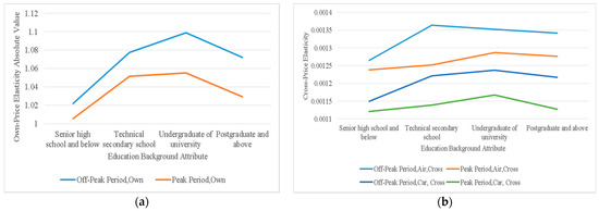
Figure 5.
The variation rules of the own- and cross-price elasticities of demand with the change in traveler’s education background attribute: (a) own-price elasticities of demand; (b) cross-price elasticities of demand.
Figure 5a shows that, on the whole, the own-price elasticities during off-peak period are larger than the ones during peak period, and the own-price elasticities of train travelers who are undergraduates are largest, and that may be because undergraduates of university usually go to university cross-province and cross-city by train and their income is low, and therefore they are more sensitive to the train price. Just like the own-price elasticities shown by Figure 5a, Figure 5b shows that the cross-price elasticities are smallest when the education level is senior high school or below; at this education level, the cross-price elasticities of demand for train and air, and train and car, change little during peak period and off-peak period, respectively. On the whole, the own and cross-price elasticities during off-peak period and peak period all showed a trend of firstly increasing and then decreasing.
Figure 6 shows the variation rules of the own- and cross-price elasticities of demand with the change in traveler’s occupation background attribute.
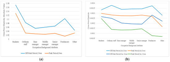
Figure 6.
The variation rules of the own- and cross-price elasticities of demand with the change in traveler’s occupation background attribute: (a) own-price elasticities of demand; (b) cross-price elasticities of demand.
Figure 6a shows that, except for freelancers, the own-price elasticities during peak period and off-peak period show a trend of firstly decreasing and then flattening or decreasing, and the own-price elasticities are largest when the respondent is a student, and that may be because many university students go to school cross-provinces or cities and their income level is usually very low, and therefore their own-price elasticities are greater. Figure 6b shows that the cross-price elasticities for train and car during peak period are smallest. The cross-price elasticities of freelancers during off-peak period are biggest; however, cross-price elasticities during peak period are small. The cross-price elasticities during peak period all show a trend of decreasing. As freelancers have more free time and travel options, during off-peak period, they are more sensitive to the price of travel mode, and during peak period, they can choose not to travel, and therefore at this time they are less sensitive to the price of the travel mode.
Figure 7 shows the variation rules of the own- and cross-price elasticities of demand with the change in traveler’s general travel distance for long-distance travel (cross-province, cross-city) attribute.
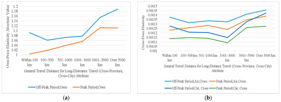
Figure 7.
The variation rules of the own- and cross-price elasticities of demand with the change in traveler’s general travel distance for long-distance travel (cross-province, cross-city) attributes: (a) own-price elasticities of demand; (b) cross-price elasticities of demand.
It can be seen from Figure 7a that during peak period, the own-price elasticities firstly increase and then decrease, and during off-peak period, the own-price elasticities firstly decrease and then increase. The own-price elasticities are biggest when the travel distance is over 5000 km, and the own-price elasticities during off-peak period are smallest when the travel distance is 100–500 km, and during peak period are smallest when the travel distance within 100 km. Figure 7b shows that cross-price elasticities during both peak period and off-peak period gradually decrease and then increase, except cross-price elasticities for train and air during peak period, which show a trend of firstly increasing and then decreasing and then increasing. The cross-price elasticities are almost smallest when the travel distance is 1001–3000 km, and the cross-price elasticities are largest when the travel distance is over 5000 km, which may be due to the fact that although train travel is common over long-distance travel, there may be a travel distance threshold for the commuter choosing long-distance train travel and, as the travel distance increases, people are more inclined to travel by other traffic modes such as by air, and more sensitive to the train fare.
Figure 8 shows the variation rules of the own- and cross-price elasticities of demand with the change in proportion of travelers’ long-distance travel (cross-province, cross-city) by train attribute.
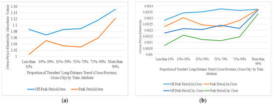
Figure 8.
The variation rules of the own- and cross-price elasticities of demand with the change in proportion of travelers’ long-distance travel (cross-province, cross-city) by train attribute: (a) own-price elasticities of demand; (b) cross-price elasticities of demand.
Figure 8a shows that the own-price elasticities during off-peak period show a trend of firstly reducing and then increasing, and during peak period they have a trend of increasing and then decreasing and then increasing; when the train travel accounted for more than 90%, the own-price elasticities were largest, when the train travel accounted for 10–30%, the minimum value of own-price elasticities during off-peak period was obtained, and when the train travel accounted for less than 10%, the one during peak period was obtained. Figure 8b shows that, on the whole, the cross-price elasticities for train and car during peak period are minimum. The cross-price elasticities are smallest when the train travel accounts for less than 10% and biggest when the train travel accounts for more than 90%, and their maximum values are almost the same. When the proportion of travelers’ long-distance travel (cross-province, cross-city) by train is biggest, travelers spend the most on train travel, and there are many relevant substitutable travel modes such as air and car, and therefore, at this time, travelers are more sensitive to the train price.
Figure 9 shows the variation rules of the own- and cross-price elasticities of demand with the change in traveler’s monthly income level attribute.
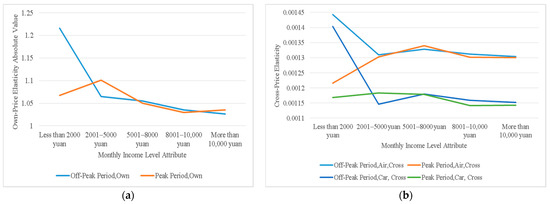
Figure 9.
The variation rules of the own- and cross-price elasticities of demand with the change in traveler’s monthly income level attribute: (a) own-price elasticities of demand; (b) cross-price elasticities of demand.
Figure 9a shows that the own-price elasticities during off-peak period tend to decrease, and the own-price elasticities during peak period firstly increase and then decrease. When the monthly income level is below 2000 yuan, the own-price elasticities during off-peak period are biggest; when the monthly income level is between 2001 and 5000 yuan, the own-price elasticities during peak period are biggest; when the monthly income level is above 10,000 yuan, the own-price elasticities are the smallest during peak period and off-peak period. Figure 9b shows that during off-peak period, the cross-price elasticities firstly decrease and then increase, and finally decrease; during peak period, the cross-price elasticities firstly increase and then decrease. When the monthly income level is below 2000 yuan, the cross-price elasticities during off-peak period are biggest. During off-peak period, as a cheaper way to travel, train is the choice of more people, especially when the travelers’ monthly income level is low, and therefore they are more sensitive to the train fare. When the monthly income level is more than 10,000 yuan, the cross-price elasticities are smallest, because these people may prefer to travel by other travel modes, such as by air, and therefore the traveler is less sensitive to the train fare.
5.3.2. Variation Rules with the Change in Influence Factors’ Influence Degree
Variation rules of the own- and cross-price elasticities of demand with the change in some typical influence factors’ influence degree during peak period and off-peak period are shown by Figure 10.
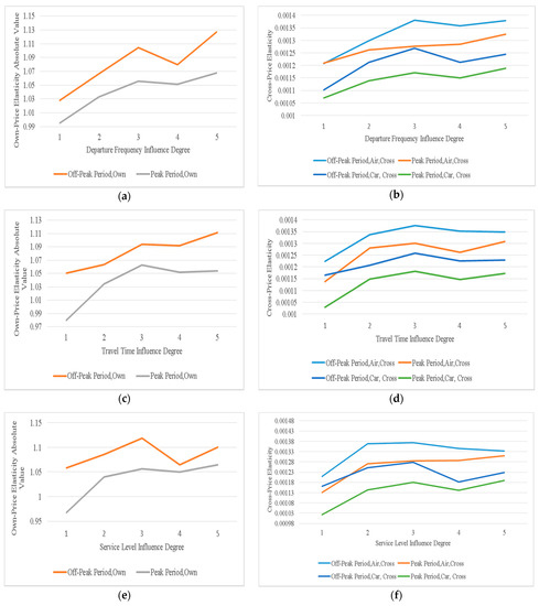
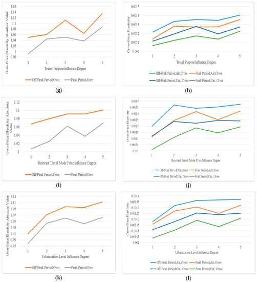
Figure 10.
Variation rules of the own- and cross-price elasticities of demand with the change in some typical influence factors influence degree during peak period and off-peak period. The (left panels) show variation rules of own-price elasticities of demand and the (right panels) show variation rules of cross-price elasticities of demand: (a,b) departure frequency influence degree; (c,d) travel time influence degree; (e,f) service level influence degree; (g,h) travel purpose influence degree; (i,j) relevant travel mode price influence degree; (k,l) urbanization level influence degree.
Figure 10 shows that the own and cross-price elasticities during off-peak period are larger than the own- and cross-price elasticities during peak period, respectively, which is consistent with the previous research, such as [2,31] and, as mentioned above, this may be because, during peak period, there are more travelers choosing to travel by train, and traffic flow is larger and travelers have fewer chances to choose other travel modes, and therefore the commuters are less sensitive to the train price. The left panels show the variation rules of the own-price elasticities of demand with the change in some typical influence factors influence degree during peak period and off-peak period, more specifically, they show that on the whole, during off-peak period and peak period, the own-price elasticities firstly increase, then decrease and then increase with the influence factors’ influence degree increasing, and have a smaller value when the influence degree is 4. When the influence degree is 3 or 5, the own-price elasticities are largest; when the influence degree is 1, the own-price elasticities are smallest. The right panels show the variation rules of the cross-price elasticities of demand with the change in some typical influence factors’ influence degree during peak period and off-peak period; more specifically, they show that on the whole, the cross-price elasticities during off-peak period and during peak period firstly increase and then decrease, and then increase slightly with the increase in influence factors’ influence degree. When the influence degree is 1, the cross-price elasticities are minimum, and when the influence degree is 3 or 5, the cross-price elasticities are maximum. Therefore, the conclusion is that when the influence degree is 3 or 5, the own- and cross-price elasticities of demand are the largest; when the influence degree is 1, the smallest own- and cross-price elasticities of demand can be obtained. Futhermore, the own-price elasticities of demand absolute values are obviously bigger than the cross-price elasticities of demand values, which is consistent with previous investigation, and Figure 10 also shows that the variation range of the own-price elasticities of demand is generally larger than the variation range of the cross-price elasticities of demand, and the cross-price elasticities of demand for train and car during peak period are almost the smallest, which indicates that the substitutability between train travel and car travel is almost minimum during peak period.
5.4. A Result Application Example: Elasticities, Energy Used and CO2 Emissions
In this section, we use a result application example to show how the elasticities of this paper can be used to reduce energy used and CO2 emissions effectively, and partly show the reliability and validity of the price elasticity of demand of this paper. For simplicity without loss of generality, we assume that the characteristics of the sample population are roughly the same as those of the travelling population, and take the cross-price elasticities for train and air as an example. Setting the train fare decreases by , we have the number of travelers switching from planes to trains as follows
where is the number of air travelers over a period of time. Set the average travel distance of travelers switching from planes to trains both by train and by plane as , and the energies used by one passenger traveling one kilometer by air and by train as and , respectively, and the CO2 emissions of one passenger traveling one kilometer by air and by train are and , respectively, and therefore, we can see that when the train fare decreases by , the reduced energy used and CO2 emissions, respectively, are
From the Ministry of Transport of China and National Bureau of Statistics of China, we have the annual data of the Chinese total aviation passenger volume and turnover, and we used the data from 2000 to 2019. Considering that train travel and air travel have a substitute relationship only in the domestic scope of China, and only Chinese domestic aviation passenger volume and turnover data for 2019 can be obtained, which are 5.86 hundred million passengers and 8520.22 hundred million passenger kilometer, respectively, and are 88.79% and 72.79% of Chinese total aviation passenger volume and turnover in 2019, respectively; therefore, in other years, we assume that the ratios of Chinese domestic aviation passenger volume and turnover to Chinese total aviation passenger volume and turnover are the same as the ones of 2019, respectively, and in a given year is the ratio of Chinese domestic aviation passenger turnover to Chinese domestic aviation passenger volume. It is difficult to distinguish the total and domestic aviation passenger volume and turnover during peak period from the ones during off-peak period, and therefore we set the cross-price elasticities for train and air as
According to Table 1, million joule per passenger kilometer and kg per passenger kilometer. Thus, we have Chinese total and domestic aviation passenger volume and turnover data from 2000 to 2019 and its calculation results about elasticities, energy used and CO2 emissions when the train fare decreases by 10% in Table 2.
Table 2.
Chinese total and domestic aviation passenger volume and turnover data from 2000 to 2019 and its calculation results about elasticities, energy used and CO2 emissions when the train fare decreases by 10%.
EJ is the energy unit and 1 EJ is equal to 1 × 10¹³ joule, and and are accurate to one passenger and one ton, respectively. are accurate to three decimal places and other variations are accurate to two decimal places when there are more than two decimal places. Table 2 shows that when the train fare reduces by 10% in China, the number of travelers switching from planes to trains is about 7823 passengers in 2000, and then increases to 77,059 passengers in 2019, and the average travel distance of travelers switching from planes to trains is from 1176 to 1454 km, which is about the distance between Beijing and Shanghai. The reduced energy used and CO2 emissions are shown by Figure 11.
Figure 11.
The reduced energy used and CO2 emissions when the train fare reduces by 10%.
Table 2 and Figure 11 show the reduced energy used and CO2 emissions when the train fare reduces by a 10% increase with time; in 2000, they were 0.176 EJ and 660 ton respectively; and in 2019, they increase to 2.118 EJ and 7955 ton, respectively; Figure 11 also shows the growth trends of the reduce energy used and CO2 emissions are roughly the same.
5.5. Discussion of Result
Based on an SP survey, this paper collected the related data and estimated the own-price elasticities of demand for train travel and the cross-price elasticities of demand for train and air, and train and car, during peak period and off-peak period, and analyzed the variation rules of own- and cross-price elasticities of demand with the change in traveler attributes and influence factors’ influence degree. However, the current study is not detailed and quantitative enough; for example, the research on the variation rules of the own- and cross-price elasticities of demand with the change in traveler attributes and influence factors’ influence degree and their variation mechanisms. Therefore, based on the data and model, more detailed and quantitative research is the direction of further research.
The study of the own-price elasticities of demand for the train travel and the cross-price elasticities of demand for train and air, and train and car, is a key determinant of investigating many related issues, such as the effects of train fare changes or train system development and expansion [1,2]. Therefore, based on the research of this paper, these problems can be studied. For example, combining the results of the paper and Chinese total and domestic aviation passenger volume and turnover data, we show how the elasticities of this paper can be used to reduce energy used and CO2 emissions effectively; considering that only Chinese domestic aviation passenger volume and turnover data for 2019 can be obtained, for simplicity without loss of generality, this example assumed that the ratios of Chinese domestic aviation passenger volume and turnover to Chinese total aviation passenger volume and turnover in other years are the same as the ones of 2019, which is also one of the further research directions. From the environmental protection perspective, this example showed when the train fare reduced by 10%, the cross-price elasticities of demand for train and air could make the air travelers switch from planes to trains to reduce energy used and CO2 emissions effectively; however, this does not mean that we should not use air travel, because air travel is fast, time-saving and safe, and so on, which we did not consider.
It is noted that, just like Gama [1], based on the data and methods, the cross-price elasticities of demand obtained in this paper are very small; for example, the cross-price elasticities of demand for train and air are 0.00128 during peak period and 0.00135 during off-peak period, and their average value is 0.001315. However, when passenger volume and turnover are very large and the train price reduces, the cross-price elasticities of demand still make many travelers switch from other travel modes to train, such as in the above example, which shows that the number of travelers switching from planes to trains is about 7823 in 2000 and then increases to 77,059 in 2019, and combined with the average travel distance of travelers switching from planes to trains in the range of 1176–1454 km, the very small cross-price elasticities of demand still can reduce energy used and CO2 emissions effectively, which also partly shows the reliability and validity of the price elasticity of demand of this paper.
Furthermore, a comparison between our results and the results of other studies in other countries can be obtained in Table 3.
Table 3.
The comparison between our results and the results of other studies in other countries.
Table 3 shows the comparison between our results and the results of other studies in other countries. For the own-price elasticities of demand, the ones of the USA are bigger than the ones of China and UK, and this may be because we estimated the price elasticity of train travel demand in the short run, and Gama [1] estimated the price elasticity of train travel demand by quarter using fixed effects by market. The ones of China are almost the same as the ones of the UK, which means that, with completely different travel preferences than in China, the own-price elasticities of this paper could be used in the UK; however, they are not suitable for America. For the cross-price elasticities of demand, the ones of the USA are bigger than the ones of China, which means that the cross-price elasticities of this paper are also not suitable for America.
6. Conclusions
This paper mainly estimates the price elasticity of train travel demand and analyzes its variation rules and application in energy used and CO2 emissions from the short-run perspective. Generally speaking, in the long run, the commuters have more time and chances to adjust their commuting behavior, such as their travel mode choice, and therefore their price elasticities of train travel demand in the long run are usually bigger than the ones in the short run. According to the above calculation and analysis, the own-price elasticities of demand are −1.049028 during peak period and −1.090438 during off-peak period, respectively. The cross-price elasticities of demand are 0.001280 for train and air and 0.001156 for train and car during peak period, and 0.001350 for train and air and 0.001230 for train and car during off-peak period.
In addition, the variation rules of own- and cross-price elasticities of demand with the change in traveler attributes and influence factors’ influence degree are different; however, the following general rules can be obtained:
- (1)
- The own and cross-price elasticities of demand during off-peak period are bigger than the ones during peak period, respectively;
- (2)
- The variation range of the own-price elasticities of demand is generally larger than the variation range of the cross-price elasticities of demand;
- (3)
- The cross-price elasticities of demand for train and car during peak period are almost the smallest;
- (4)
- As influence factors’ influence degree increases, on the whole, the own- and cross-price elasticities of demand firstly increase and then decrease, and finally increase. When the influence degree is 3 or 5, the own- and cross-price elasticities of demand are largest; when the influence degree is 1, the own- and cross-price elasticities of demand are smallest.
Finally, a result application example showed that the elasticities of this paper could be used to reduce energy used and CO2 emissions effectively; however, this does not mean that we should not use the air, because besides the environmental protection, there are many other factors to consider.
Author Contributions
Conceptualization, Y.Z.; data curation, Y.Z.; formal analysis, Y.Z.; funding acquisition, Y.Z. and X.Y.; investigation, Y.Z.; methodology, Y.Z.; supervision, B.R. and N.Z.; writing—original draft, Y.Z.; writing—review and editing, Y.Z. and X.Y. All authors have read and agreed to the published version of the manuscript.
Funding
This study was funded and supported by several projects: the National Natural Science Foundation of China (Grant No. 91746201 and 71621001); Youth Foundation for Humanities and Social Sciences Research, Ministry of Education of China (Grant No. 19YJC630007); the Natural Science Foundation of Jiangsu Province of China (Grant No. BK20180898); the Natural Science Foundation of the Jiangsu Higher Education Institutions of China (Grant No. 18KJB580017); Science and Technology Innovation Incubation Fund of Yangzhou University (Grant No. 2019CXJ057).
Informed Consent Statement
Informed consent was obtained from all subjects involved in the study.
Data Availability Statement
The data presented in this study are available on request from the corresponding author. The data are not publicly available due to privacy.
Conflicts of Interest
The authors declare no conflict of interest.
References
- Gama, A. Own and cross-price elasticities of demand for domestic flights and intercity trains in the U.S. Transp. Res. Part D 2017, 54, 360–371. [Google Scholar] [CrossRef]
- Grange, L.; de González, F.; Muñoz, J.C.; Troncoso, R. Aggregate estimation of the price elasticity of demand for public transport in integrated fare systems: The case of Transantiago. Transp. Policy 2013, 29, 178–185. [Google Scholar] [CrossRef]
- Chen, B.Y.; Jiang, M.Q.; Si, B.F.; Yang, X.B. Empirical analysis of demand-price elasticity for urban public transit in multimodal transport system. J. Transp. Syst. Eng. Inf. Technol. 2016, 4, 241–247. (In Chinese) [Google Scholar]
- Gao, Y.F.; Si, B.F. Optimal algorithm and empirical analysis for urban transit pricing based on demand elasticity. J. Transp. Syst. Eng. Inf. Technol. 2019, 3, 163–168. (In Chinese) [Google Scholar] [CrossRef]
- Goodwin, P. A review of new demand elasticities with special reference to short and long run effects of price changes. J. Transp. Econ. Policy 1992, 26, 155–171. [Google Scholar] [CrossRef]
- Crôtte, A.; Noland, R.B.; Graham, D.J. Is the Mexico City metro an inferior good? Transp. Policy 2009, 16, 40–45. [Google Scholar] [CrossRef]
- García-Ferrer, A.; Bujosa, M.; Juan, A.D.; Poncela, P. Demand forecast and elasticities estimation of public transport. J. Transp. Econ. Policy 2006, 40, 45–67. [Google Scholar]
- Paulley, N.; Balcombe, R.; Mackett, R.; Titheridge, H.; Preston, J.M.; Wardman, M.R.; Shires, J.D.; White, P. The demand for public transport: The effects of fares, quality of service, income and car ownership. Transp. Policy 2006, 13, 295–306. [Google Scholar] [CrossRef]
- Melo, P.C.; Sobreira, N.; Goulart, P. Estimating the long-run metro demand elasticities for Lisbon: A time-varying approach. Transp. Res. Part A 2019, 126, 360–376. [Google Scholar] [CrossRef]
- Mumbower, S.; Garrow, L.A.; Higgins, M.J. Estimating fight-level price elasticities using online airline data: A first step toward integrating pricing, demand, and revenue optimization. Transp. Res. Part A 2014, 66, 196–212. [Google Scholar] [CrossRef]
- Perera, S.; Tan, D. In search of the “Right Price” for air travel: First steps towards estimating granular price-demand elasticity. Transp. Res. Part A 2019, 130, 557–569. [Google Scholar] [CrossRef]
- Anciaes, P.; Metcalfe, P.; Heywood, C.; Sheldon, R. The impact of fare complexity on rail demand. Transp. Res. Part A 2019, 120, 224–238. [Google Scholar] [CrossRef]
- Wardman, M. Price elasticities of surface travel demand-a meta-analysis of UK evidence. J. Transp. Econ. Policy 2014, 48, 367–384. [Google Scholar]
- Berry, S. Estimating discrete choice models of product differentiation. RAND J. Econ. 1994, 25, 242–262. [Google Scholar] [CrossRef]
- Hensher, D.A.; Bullock, R.G. Price elasticity of commuter mode choice: Effect of a 20 percent rail fare reduction. Transp. Res. Part A 1979, 3, 193–202. [Google Scholar] [CrossRef]
- Nowak, W.P.; Savage, I. The cross-price elasticity between gasoline prices and transit use: Evidence from Chicago. Transp. Policy 2013, 29, 38–45. [Google Scholar] [CrossRef]
- Ignacio, E.R. The elasticities of passenger transport demand in the Northeast Corridor. Res. Transp. Econ. 2019, 78, 100759. [Google Scholar] [CrossRef]
- Li, Z.; Hensher, D.A.; Rose, J.M. Identifying sources systematic variation in direct price elasticities from revealed preference studies of inter-city freight demand. Transp. Policy 2011, 18, 727–734. [Google Scholar] [CrossRef]
- Sipes, K.N.; Mendelsohn, R. The effectiveness of gasoline taxation to manage air pollution. Ecol. Econ. 2001, 36, 299–309. [Google Scholar] [CrossRef]
- Hössinger, R.; Link, C.; Sonntag, A.; Stark, J. Estimating the price elasticity of fuel demand with stated preferences derived from a situational approach. Transp. Res. Part A 2017, 103, 154–171. [Google Scholar] [CrossRef]
- Hensher, D.A.; Rose, J.M. Bridging research and practice: A synthesis of best practices in travel demand modeling. Transp. Res. Part A 2007, 41, 428–443. [Google Scholar] [CrossRef]
- Mabit, S.L.; Fosgerau, M. Demand for alternative-fuel vehicles when registration taxes are high. Transp. Res. Part D 2011, 16, 225–231. [Google Scholar] [CrossRef]
- Cervero, R. Transit pricing research. Transportation 1990, 17, 117–139. [Google Scholar] [CrossRef]
- Taplin, J.H.E.; Hensher, D.A.; Smith, B. Preserving the symmetry of estimated commuter travel elasticities. Transp. Res. Part B 1999, 33, 215–232. [Google Scholar] [CrossRef]
- Raghoo, P.; Surroop, D. Price and income elasticities of oil demand in Mauritius: An empirical analysis using cointegration method. Energy Policy 2020, 140, 111400. [Google Scholar] [CrossRef]
- Caldara, D.; Cavallo, M.; Iacoviello, M. Oil price elasticities and oil price fluctuations. J. Monetary Econ. 2019, 103, 1–20. [Google Scholar] [CrossRef]
- Liddle, B.; Smyth, R.; Zhang, X. Time-varying income and price elasticities for energy demand: Evidencefrom a middle-income panel. Energ. Econ. 2020, 86, 104681. [Google Scholar] [CrossRef]
- Teng, M.; Burke, P.J.; Liao, H. The demand for coal among China’s rural households: Estimates of price and income elasticities. Energ. Econ. 2019, 80, 928–936. [Google Scholar] [CrossRef]
- Cardoso, L.C.B.; Bittencourt, M.V.L.; Litt, W.H.; Irwin, E.G. Biofuels policies and fuel demand elasticities in Brazil. Energy Policy 2019, 128, 296–305. [Google Scholar] [CrossRef]
- Zhao, H.L.; Zhang, N. Who is the main influencer on safety performance of dangerous goods air. Transportation in China? J. Air Transp. Manag. 2019, 75, 198–203. [Google Scholar] [CrossRef]
- Mayeres, I. Efficiency effects of transport policies in the presence of externalities and distortionary taxes. J. Transp. Econ. Policy 2000, 34, 233–260. [Google Scholar]


Publisher’s Note: MDPI stays neutral with regard to jurisdictional claims in published maps and institutional affiliations. |
© 2021 by the authors. Licensee MDPI, Basel, Switzerland. This article is an open access article distributed under the terms and conditions of the Creative Commons Attribution (CC BY) license (http://creativecommons.org/licenses/by/4.0/).