Analytical Models for Seawater and Boron Removal through Reverse Osmosis

Abstract

Regarding the purification of seawater, it is necessary to reduce both the total concentration of salt and also the concentration of boron to meet purity requirements for safe drinking water. For this purpose reverse osmosis membrane modules can be designed based on experimental data supported by computer models to determine energy efficient configurations and operating conditions. In previous studies numerical models have been suggested to predict the performance of the removal with respect to difference pressures, pH values, and temperatures. Here, an analytical model is suggested which allows for both the simplified fitting of the parameters required for predicting boron transport coefficients and also the simple equations that can be used for the design of combined seawater and boron removal systems. This modelling methodology is demonstrated through two case studies including FilmTec and Saehan membrane modules. For both cases the model is shown to be able to predict the performance with similar accuracy compared with existing finite-difference type numerical models from the literature.

1. Introduction

Due to global population growth and the spread of pollution it is becoming more challenging to provide clean drinking. A sustainable method for obtaining clean water is through seawater desalination by reverse osmosis. A reverse osmosis membrane system is composed of high-pressure pumps, one or more reverse osmosis membranes, and energy recovery devices which are designed to meet purity requirements while also minimizing energy consumption. The pressure of the seawater supplied by the high-pressure pump varies depending on the salt concentration of the seawater. The standard criteria in the seawater desalination process is the concentration of TDS (total dissolved solids) and boron in fresh water. The WHO (World Health Organization) states that the palatability of water with TDS lower than 600 mg/L is considered good and they specify guidelines for 2.4 mg/L of boron [1], although lower values are generally preferred. These WHO criteria have an impact on the design of the seawater reverse osmosis (SWRO) processes such that both salt rejection and boron rejection must be considered.

The removal of boron through reverse osmosis is complicated by the fact that boron exists in seawater mainly as boric acid and borate ions (with negligible concentrations of other boron compounds) [2]. This is a problem because reverse osmosis membranes are known to easily permeate only the negatively charged borate ions while having more difficulty removing the neutrally charged boric acid [3]. For this reason the pH should typically be increased to give higher fractions of borate ions [2]. This has been demonstrated using FilmTec membranes which are shown to give very high boron rejection at high pH values [4]. Additionally, Koseoglu et al. tested FilmTec and Toray membranes and found that around 85–90% rejection is possible at pH 8.2 while pH 11 allows for 98% or higher rejection using both membranes [5]. More recently Ali et al. have developed a membrane material which is able to achieve 99% boron rejection at pH 10 [6]. At a lower pH of 8 Li et al. have developed a membrane modification process which embeds 4-nitrobenzenesulfonyl chloride into an existing membrane and is able to increase the boron rejection from 82.12% up to 93.1% [7]. In addition to the development of new materials, the design of feed spacers inside the membrane modules is also important. A review of the impact of feed spacer design by Haidari et al. discusses their effects on pressure drop, flux through the membrane, and fouling [8]. Additionally, it is suggested by Ruiz-Garcia and Nuez based on experimental and modelling results that feed spacers should be chosen based on the designed operating conditions to reduce energy consumption and enhance the quality of the permeate [9].

In order to meet boron drinking water criteria, a multistage design of reverse osmosis modules is typically required [2]. For example, Tu et al. state that in practice a first stage with natural pH might be used to reduce TDS and a second stage with elevated pH might be used to remove boron [10]. In addition to reverse osmosis, Najid et al. consider and discuss alternative technologies for boron removal including electrocoagulation, adsorption, ion exchange, and various other membrane processes such as forward osmosis and membrane distillation [2]. Their comparison showed that reverse osmosis has the potential to remove boron but can be uneconomical due to high energy requirements and the requirement to alter pH, and hence they suggest that a hybrid process combining different technologies could be the best solution [2]. To reduce the costs of two-stage processes Ban et al. also consider a hybrid process with one stage of forward osmosis followed by a second stage with reverse osmosis [11]. They compare this against a two-stage reverse osmosis design and show that the costs associated with chemically altering the pH can be eliminated by using the hybrid forward osmosis plus reverse osmosis process, but this comes at the expense of higher capital costs [11]. Instead of chemical modification Jung et al. have suggested electrochemical modification using a layer of carbon nanotubes on the membrane surface as a cathode to increase the pH. While this does increase boron rejection over 90% it also causes some scaling [12]. In another recent study a hybrid system is suggested combining electro dialysis as a pretreatment with a nanofiltration reverse osmosis to enhance the overall boron removal [13].

Despite this progress in membrane materials and potential hybrid systems there is still the need for modelling and optimization of such systems. This would allow, for example, the prediction of salt and boron rejection for wide ranges of possible conditions to identify low energy and low cost designs. For example, Ruiz-Garcia et al. use modelling to compare the performance of two different Toray membranes (TM820L-440 and TM820S-400) for the purpose of boron removal over a range of conditions and show that the TM820L-440 generally gives lower boron concentrations of under 1ppm [14].

Modelling can also be used to simulate and compare different configurations of separators to further enhance energy efficiency. For example, Al-Obaidi et al. evaluated the performance of a multistage reverse osmosis system with varying operating parameters through a modelling approach [15]. In other work Al-Obaidi et al. also utilized modelling to compare a number of different recycling options in a multistage reverse osmosis membrane process [16]. More recently Alsarayreh et al. also used a modelling approach to investigate different retentate recycle ratios [17].

The review of Alsarayreh et al. shows that a larger number of models have been developed for the prediction of performance for spiral wound reverse osmosis membrane modules [18]. These models can be divided into two categories: numerical models which discretize the length of the module and formulate model equations using finite difference type methods, and analytical models which use integration of model equations to obtain expressions for directly calculating the outlet conditions. While the majority of models developed have been for steady state solutions, model equations can also be solved dynamically as shown by Joseph and Damodaran [19]. Regarding steady state modelling, Ben Boudinar et al. have developed a numerical model solved through finite differences and they show that their model fits well for desalination of brackish water but is less accurate for seawater desalination [20]. They suggest that this is due to an inaccuracy in the mass transfer coefficient [20]. This has been addressed by Senthilmurugan et al. who also fitted parameters for mass transfer correlations as well as solving the model equations using finite differences [21]. In other studies, such as the work of Geraldes et al., mass transfer correlations for “typical spiral wound modules” are assumed to be valid [22]. While Geraldes et al. do not provide validation for their model they have fitted water and salt transport coefficients which are then used to optimize the configuration and operating conditions of a two-stage desalination system [22].

Following these works numerical models have also been developed to predict the removal of boron. For example, the study of Mane et al. developed a finite elements model to predict the removal of boron [23]. In that study the parameters and correlations for boron transport coefficients developed by Hyung and Kim based on experimental results are used to account for the effects of pH and temperature [24]. Another study of Ruiz-Garcia et al. proposed a function for boron permeability in terms of feed pressure, temperature, and operating time based on plant data which might also be used in modelling studies [25]. Alternatively the model developed by Sassi et al. [26] used a finite-difference type numerical model which accounts for boron permeation using data and correlations from the experimental study of Taniguchi et al. [27]. More recently the study of Du et al. [28] also considered boron removal through numerical models based on a combination of the equations from the studies of Geraldes et al. [22] and Hyung and Kim [24] which they use to optimize a superstructure of different configurations.

A number of studies have also developed analytical models where the model equations are integrated to give analytical expressions. For example, Avlonitis et al. developed equations for calculating the variation of concentration, pressure, and flow rates along the length of the module, although they assume that the mass transfer coefficient is constant along the length [29]. More recently Sundaramoorthy et al. suggested an analytical model which includes the variation of the mass transfer coefficient across the length [30]. They have demonstrated the validity of their approach through the removal of chlorophenol [31] and dimethylphenol [32] from waste water where they show how model parameters and parameters for mass transfer coefficients can be estimated through linear fitting of experimentally measured values. Following these earlier studies an analytical model was developed by Fraidenraich et al. for the desalination of brackish water which they showed to be accurate for the conditions tested [33]. Additionally, Al-Obaidi et al. have published numerous models including the development of analytical expressions from integration [34] and using average pressure and salt concentrations to simplify calculations which can be used to evaluate and test different configurations of modules [35].

While great progress has been made simulating desalination membrane modules using finite-difference type numerical models, these models generally involve large numbers of equations (due to the discretization) which can be solved simultaneously or possibly sequentially using numerical algorithms. Meanwhile, analytical models will have a relatively small number of equations which can be solved using less computational time and simpler algorithms; for example, in a spreadsheet program. Hence, analytical models should be more suitable for the design and optimization of multistage configurations which require the simulation of individual module performance a large number of times, provided they are shown to give reasonable accuracy.

However, to the best of our knowledge, there has not been any analytical model (based on integration of model equations) which has been developed to predict the removal of both salt and boron simultaneously. Therefore, for this reason, a combined salt and boron removal analytical model is developed here. Additionally, in many cases the fitting of parameters for spiral wound reverse osmosis models are often proposed based on nonlinear optimization using least-squares methods. In this study the methods of Sundaramoorthy et al. [30] and Avlonitis et al. [29] are extended such that all the model parameters can be estimated though simpler linear optimization in a new sequential parameter estimation procedure.

2. Development of a New Analytical Model for Predicting Salt and Boron Removal

The modelling equations given here are based on the method suggested by Sundaramoorthy et al. [30,31], who developed a model for the removal of organic solutes using spiral wound reverse osmosis membranes. Here, this model is modified in the following ways:

• Modified to use for seawater purification;
• Estimation of pressure drop coefficients for cases where outlet pressure is not measured;
• Including temperature dependence of water and salt transport coefficients;
• Including equations for boron transport.

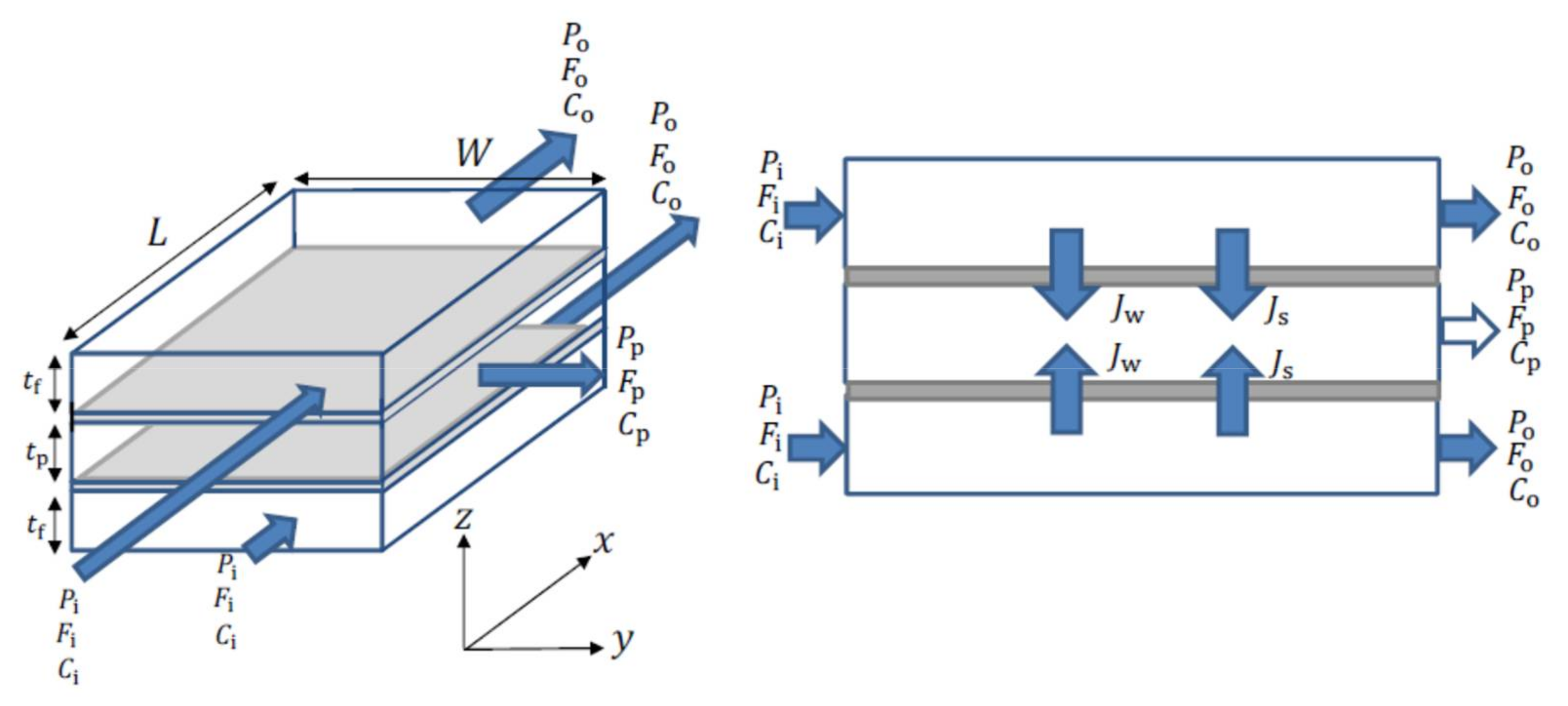
2.1. Modelling Equations

The transport of water and salts through a membrane are typically described according to the solution–diffusion model which can be used to calculate the flux of water $\left(J_{\mathrm{W}}\right)$ and salt $(J_{\mathrm{S}})$:

$$J_{\mathrm{W}}=A_{\mathrm{w}}\left(\Delta P-\Delta \pi \right)$$

(1)

$$J_{\mathrm{S}}=B_{\mathrm{S}}\left(C_{\mathrm{b}}-C_{\mathrm{p}}\right)$$

(2)

where $\Delta P$ and $\Delta \pi$ are the transmembrane pressure and osmotic pressure, and $C_{\mathrm{b}}$ and $C_{\mathrm{p}}$ are the brine-side and permeate-side concentrations of salt. $A_{\mathrm{w}}$ and $B_{\mathrm{S}}$ are the water and salt transport coefficients.

Accounting for the effect of concentration polarization which causes the concentration of salt to increase at the membrane surface, these equations should be modified to use the concentration of salt at the membrane wall $\left(C_{\mathrm{w}}\right)$. The concentration at the membrane wall can be calculated based on the following relation [30]:

$$\frac{C_{\mathrm{w}}-C_{\mathrm{p}}}{C_{\mathrm{b}}-C_{\mathrm{p}}}=exp\left(\frac{J_{\mathrm{W}}}{k}\right)$$

(3)

where k is the mass transfer coefficient and so that Equation (2) is modified:

$$J_{\mathrm{S}}=B_{\mathrm{S}}\left(C_{\mathrm{w}}-C_{\mathrm{p}}\right)$$

(4)

The pressure drop can be estimated based on Darcy’s law which might be written as [30]:

$$\frac{dP}{dx}=bF\left(x\right)$$

(5)

which gives the pressure drop as a function of volume flow rate multiplied by a fixed parameter $b$. Alternatively, if knowledge about feed spacer geometry is available, pressure drop can also be estimated using more complex equations suggested by Koutsou et al. [36].

The osmotic pressure is a function of salt concentration and temperature. For low concentrations, such as those used in seawater, it may be approximated by the van’t Hoff relation in Equation (6). Thus the transmembrane osmotic pressure can be calculated using Equation (7):

$$\pi =i\gamma TC$$

(6)

$$\Delta \pi =i\gamma T\left(C_{\mathrm{w}}-C_{\mathrm{p}}\right)$$

(7)

where $\gamma$ is the gas law constant, T is temperature, and i is the number of ionic species formed. For the organic solutes considered by Sundaramoorthy, i is equal to 1 [31,32] but for NaCl the value of i is 2.

Combining and rearranging the above equations, the flux of water and the permeate salt concentration can be calculated as follows:

$$J_{\mathrm{W}}=\frac{A_{\mathrm{w}}\Delta P}{1+\left(\frac{A_{\mathrm{w}}i\gamma }{B_{\mathrm{S}}}\right)T{C}_{\mathrm{p}}}$$

(8)

$$C_{\mathrm{p}}=\frac{C_{\mathrm{b}}}{\left[1+\frac{\left(\raisebox{1ex}{$J_{\mathrm{W}}$}\!\left/ \!\raisebox{-1ex}{$B_{\mathrm{s}}$}\right.\right)}{exp\left(\raisebox{1ex}{$J_{\mathrm{W}}$}\!\left/ \!\raisebox{-1ex}{$k$}\right.\right)}\right]}$$

(9)

The above equations can also be modified using a reflection coefficient, but for simplicity this will be assumed to be equal to 1.

To estimate the transport flux of boron an expression similar to Equation (4) can be used:

$$J_{\mathrm{B}}=B_{\mathrm{B}}\left(C_{\mathrm{Bw}}-C_{\mathrm{Bp}}\right)$$

(10)

where $B_{\mathrm{B}}$ is the boron transport coefficient and $C_{\mathrm{Bw}}-C_{\mathrm{Bp}}$ is the difference in boron concentrations. The wall concentration of boron can also be estimated with an equation similar to Equation (3) which also requires a mass transfer coefficient $k_{\mathrm{B}}$:

$$\frac{C_{\mathrm{Bw}}-C_{\mathrm{Bp}}}{C_{\mathrm{Bb}}-C_{\mathrm{Bp}}}=exp\left(\frac{J_{\mathrm{W}}}{k_{\mathrm{B}}}\right)$$

(11)

$$C_{\mathrm{Bp}}=\frac{C_{\mathrm{Bb}}}{\left[1+\frac{\left(\raisebox{1ex}{$J_{\mathrm{W}}$}\!\left/ \!\raisebox{-1ex}{$B_{\mathrm{B}}$}\right.\right)}{exp\left(\raisebox{1ex}{$J_{\mathrm{W}}$}\!\left/ \!\raisebox{-1ex}{$k_{\mathrm{B}}$}\right.\right)}\right]}$$

(12)

$$B_{\mathrm{B}}=\frac{\left\{H^{+}\right\}}{\left\{H^{+}\right\}+K_{\mathrm{a}1}}{B}_{\left({\mathrm{H}}_3{\mathrm{BO}}_3\right)0}{e}^{\left(0.067\left(T-T_0\right)\right)}+\frac{K_{a1}}{\left\{H^{+}\right\}+K_{\mathrm{a}1}}{B}_{\left({\mathrm{H}}_2{\mathrm{BO}}_3{}^{-}\right)0}{e}^{\left(0.049\left(T-T_0\right)\right)}$$

(13)

To estimate the boron transport coefficients Hyung and Kim [24] proposed Equation (13) where they found the temperature dependence follows the same trend for all the membranes they tested. The effect of pH is included through the calculation of the fraction of boric acid $\left({\mathrm{H}}_3{\mathrm{BO}}_3\right)$ and borate ion $\left({\mathrm{H}}_2{\mathrm{BO}}_3{}^{-}\right)$ which have different transport coefficients: $B_{\left({\mathrm{H}}_3{\mathrm{BO}}_3\right)0}$ and $B_{\left({\mathrm{H}}_2{\mathrm{BO}}_3{}^{-}\right)0}$ (the values at $T=T_0$).

Various correlations have been proposed in the literature for estimating the mass transfer coefficient, although in most cases these correlations predict the Sherwood number $\left(sh\right)$ as a function of the feed-side Reynolds number $\left(R{e}_{\mathrm{f}}\right)$ and Schmidt number $\left(Sc\right)$ and also sometimes consider the permeate-side Reynolds number $\left(R{e}_{\mathrm{p}}\right)$ [31]. In this study the following general expression is considered:

$$sh=e^A \left(R{e}_{\mathrm{f}}{}^B\right) \left(R{e}_{\mathrm{p}}{}^C\right) \left(S{c}^D\right)$$

(14)

To model the performance of a spiral wound reverse osmosis membrane for purification of seawater and boron, we made the following assumptions:

• Pressure drop is neglected in the permeate side;
• Darcy’s law applies for pressure drop in the feed side;
• Validity of the solution–diffusion equations;
• Feed-side: velocity in the y and z directions is neglected;
• Permeate-side: velocity in the x and z directions is neglected;
• The unwound spiral can be represented by the diagram in Figure 1;
• The boron mass transfer coefficient is the same as that used for salt.

Based on these assumptions, Sundarmoorthy et al. showed that analytical solutions can be obtained for the pressure $P$, volume flow rate $F$, and water flux $J_{\mathrm{W}}$ [30,31]. The permeate-side fluid velocities are much lower than those on the retentate side and thus the permeate-side pressure drop should be significantly lower, which is why it is often neglected, allowing for the development of Equations (15)–(19) [30]. Additionally, it has been shown by Taniguchi et al. that the mass transfer coefficient for salt is very close to that of boron and so for simplicity they are considered equal in this study [27]. The equations for pressure and volume flow can be used to calculate the outlet pressure and outlet volume flow rate as given below:

$$F_{\mathrm{o}}=F_{\mathrm{i}}\cosh \varphi -\frac{\varphi \sinh \varphi }{bL}\mathsf{\Delta }{P}_{\mathrm{i}}$$

(15)

$$P_{\mathrm{o}}=P_{\mathrm{i}}-\frac{bL}{\varphi \sinh \varphi }\left[\left(F_{\mathrm{i}}+F_{\mathrm{o}}\right)\left(\cosh \left(\varphi \right)-1\right)\right]$$

(16)

$$C_{\mathrm{o}}=C_{\mathrm{p}}+\frac{F_{\mathrm{i}}\left(C_{\mathrm{i}}-C_{\mathrm{p}}\right)}{F_{\mathrm{o}}}\cosh \varphi -\frac{\varphi \sinh \varphi }{bL}\mathsf{\Delta }{P}_{\mathrm{i}}$$

(17)

where $\mathsf{\Delta }{P}_{\mathrm{i}}=P_{\mathrm{i}}-P_{\mathrm{p}}$ is the transmembrane pressure at the inlet and the $\varphi$ is given by the following equation:

$$\varphi =L\sqrt{\frac{Wb{A}_{\mathrm{w}}}{\left(1+A_{\mathrm{w}}\left(\frac{i\gamma }{B_{\mathrm{S}}}\right)T{C}_{\mathrm{p}}\right)}}$$

(18)

This parameter $\varphi$ is a dimensionless number which is defined by Sundaramoorthy et al. in the following equation relating the second order derivative of the feed channel volume flow rate with respect to distance along the module [30]:

$$\frac{d^{2}F\left(x\right)}{dx}=\frac{{\varphi }^2}{L^2}F\left(x\right)$$

(19)

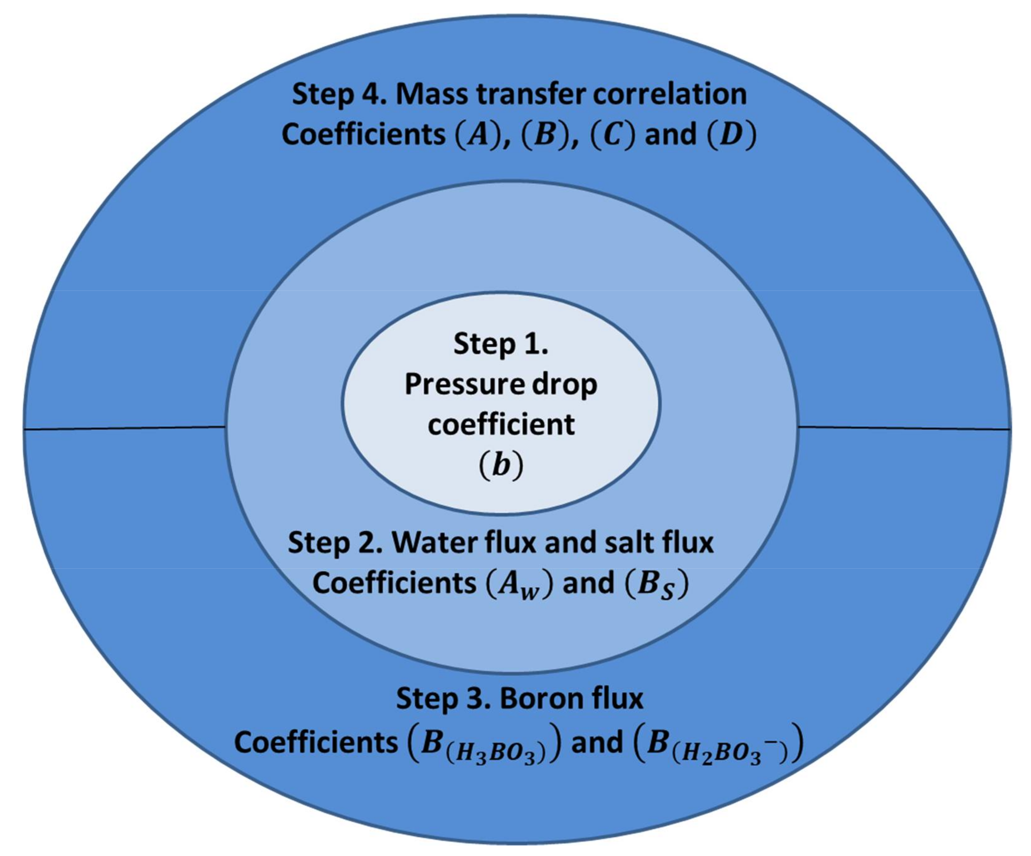
2.2. Parameter Estimation

Based on the above equations a number of parameters need to be fit in order to model the performance of the spiral wound reverse osmosis membrane for the prediction of salt and boron removal. Hence, in this study we suggest the sequential procedure of parameter fitting steps as given in Figure 2. Sundaramoorthy et al. [30,31] suggested procedures for steps 1, 2, and 4 where they suggest linear fitting for steps 1 and 2 and a least-squares (presumably nonlinear) fitting for step 4. Additionally, in step 2 they assumed that $A_{\mathrm{w}}$ and $B_{\mathrm{S}}$ are fixed and do not change with temperature.

In the procedure shown in Figure 2, the first step should be to estimate pressure drop. Subsequently the water and salt transport coefficients $A_{\mathrm{w}}$ and $B_{\mathrm{S}}$ should be estimated for each inlet temperature such that the temperature dependence can be predicted. Steps 3 and 4 are independent of each other but both rely on parameters fitted in steps 1 and 2. All of these steps can be realized through linear fitting using experimentally measured values.

2.2.1. Step 1. Pressure Drop Parameter Estimation

As mentioned above the pressure drop on the feed/brine side can be estimated through Darcy’s law as given by Equation (5) which is written in terms of the volume flow. However, this can also be written as [21]:

$$\frac{dP}{dx}=k_{\mathrm{fb}}\mu v_{\mathrm{f}}{}^{n_{\mathrm{f}}}$$

(20)

where $v_{\mathrm{f}}$ is the feed-side fluid velocity, $\mu$ is the fluid viscosity, $k_{\mathrm{fb}}$ is a friction parameter, and $n_{\mathrm{f}}$ is a constant which is commonly assumed to be 1, although some studies have considered other values. For example, Sentilmurugan at al. also considered $n_{\mathrm{f}}=1.5$ and found that changing this value only had a small effect on results [21]. In this study it is assumed $n_{\mathrm{f}}=1$ and hence Equation (20) is equivalent to Equation (5).

The estimation of $b$ is possible through plotting $P_{\mathrm{o}}-P_{\mathrm{i}}$ against $\frac{L}{\varphi \sinh \varphi }\left[\left(F_{\mathrm{i}}+F_{\mathrm{o}}\right)\left(\cosh \left(\varphi \right)-1\right)\right]$ (from Equation (16)) and fitting a linear expression should give $b$ as the gradient, as suggested by Sundaramoorthy et al. [30,31].

However, this requires knowledge of the feed/brine side outlet pressure which may not be provided or possibly not measured as part of experimental studies looking at reverse osmosis desalination. In these cases the pressure drop might be estimated based on the maximum pressure drop specified by the manufacturer. For example, we might estimate that the highest flow rate tested experimentally gives a pressure drop which is 100% of the maximum:

$$b=\frac{P_{\mathrm{dropmax}}}{L{F}_{\mathrm{i},\max }}$$

(21)

Alternatively, if a friction factor is available the value of $b$ can be readily found:

$$b=\frac{k_{\mathrm{fb}}\mu }{A_{\mathrm{f}}}$$

(22)

where $A_{\mathrm{f}}$ is the cross sectional area of the feed channel and the viscosity is calculated for a single typical experimental inlet value.

2.2.2. Step 2. Water and Salt Transport Parameter Estimation

The values of coefficients $A_{\mathrm{w}}$ and $B_{\mathrm{S}}$ can be estimated based on the equations given by Sundaramoorthy et al. which are as follows [30,31]:

$$\varphi ={\cosh }^{-1}\left[\frac{\left(F_{\mathrm{i}}+F_{\mathrm{o}}\right)-\beta F_{\mathrm{o}}}{\left(F_{\mathrm{i}}+F_{\mathrm{o}}\right)-\beta F_{\mathrm{i}}}\right]$$

(23)

$$\beta =\frac{P_{\mathrm{i}}-P_{\mathrm{o}}}{P_{\mathrm{i}}-P_{\mathrm{p}}}$$

(24)

The value of $\varphi$ can be calculated directly from inlet and outlet volumetric flow rates and pressures. Hence, a plot of $1/{\varphi }^2$ against $T{C}_{\mathrm{p}}$ should give a linear fitting which can be used to calculate the values of $A_{\mathrm{w}}$ and $B_{\mathrm{S}}$:

$$\frac{1}{{\varphi }^2}=\left(\frac{i\gamma }{L^{2}Wb{B}_{\mathrm{S}}}\right)T{C}_{\mathrm{p}}+\left(\frac{1}{L^{2}Wb{A}_{\mathrm{w}}}\right)$$

(25)

This is the same as the equation given by Sundaramoorthy et al. [30,31] except with the addition of i to account for the presence of NaCl.

If the outlet pressures $P_{\mathrm{o}}$ are not measured then this can be estimated using the fitted $b$ value and the following approximate expression:

$$P_{\mathrm{i}}-P_{\mathrm{o}}=Lb\frac{\left(F_{\mathrm{i}}+F_{\mathrm{o}}\right)}{2}$$

(26)

It is also worth noting that the above fitting should utilize the inlet and outlet conditions for a single feed channel, accounting for the number of leaves and the number of feed channels per leaf. Additionally, while Sundaramoorthy et al. [30,31] assume the fitted constants are independent of temperature, this fitting can also be performed separately for each set of data at each temperature which can then be used to fit a temperature dependent term. For example, Arrhenius-type equations can be used [23,37]:

$$A_{\mathrm{w}}=A_{\mathrm{w}0}exp\left[\frac{-E_{\mathrm{A}}}{R}\left(\frac{1}{T}-\frac{1}{T_0}\right)\right]$$

(27)

$$B_{\mathrm{S}}=B_{\mathrm{S}0}exp\left[\frac{-E_{\mathrm{B}}}{R}\left(\frac{1}{T}-\frac{1}{T_0}\right)\right]$$

(28)

where $E_{\mathrm{A}}$ and $E_{\mathrm{B}}$ are apparent activation energies, $R$ is the gas constant, and $A_{\mathrm{w}0}$ and $B_{\mathrm{S}0}$ are the values of water and salt transport coefficients at temperature $T_0$. The above equations can be used to evaluate the values at other temperatures. Although Arrhenius equations are more commonly associated with chemical reactions, Mehdizadeh et al. have shown that this type of relation also works well for predicting fluxes through membranes at different temperatures as they argue it is a similar phenomenological process [37].

2.2.3. Step 3. Boron Transport Parameter Estimation

The transport coefficients of boron can be estimated based on the following equation suggested by Hyung and Kim which accounts for the transport of boric acid $\left({\mathrm{H}}_3{\mathrm{BO}}_3\right)$ and borate ion $\left({\mathrm{H}}_2{\mathrm{BO}}_3{}^{-}\right)$ [24]:

$$B_{\mathrm{B}}={\alpha }_0{B}_{\left({\mathrm{H}}_3{\mathrm{BO}}_3\right)}+{\alpha }_1{B}_{\left({\mathrm{H}}_2{\mathrm{BO}}_3{}^{-}\right)}$$

(29)

In this equation, ${\alpha }_0$ and ${\alpha }_1$ represent the fractions of boric acid and borate ion which can be estimated using the apparent dissociation constant $K_{\mathrm{a}1}$ and the $H^{+}$ ion concentration [24]:

$${\alpha }_0=\frac{\left\{H^{+}\right\}}{\left\{H^{+}\right\}+K_{\mathrm{a}1}}$$

(30)

$${\alpha }_1=\frac{K_{\mathrm{a}1}}{\left\{H^{+}\right\}+K_{\mathrm{a}1}}$$

(31)

The value of $K_{\mathrm{a}1}$ can be determined by a correlation in terms of salt concentration and temperature as given by the correlation of Edmond and Gieskes as presented by Nir and Lahav [38]:

$${\log }_{10}{K}_{\mathrm{a}1}=\frac{2291.90}{T}+0.01756T-3.3850-0.32051{\left(\frac{S}{1.80655}\right)}^{\raisebox{1ex}{$1$}\!\left/ \!\raisebox{-1ex}{$3$}\right.}$$

(32)

where $T$ is the temperature in kelvin, and $S$ is the concentration of salt in g/L. It was also noted by Nir and Lahav [38] that a number of authors have missed the temperature dependence from the $0.01756 T$ term when writing this correlation.

Although in principle the temperature dependent factors can also be estimated here through fitting expressions similar to Equation (27), the temperature-dependent expressions determined by Hyung and Kim can also be used since they show that their fitted parameters fit well for a number of different membranes tested [24]. The work of Hyung and Kim also gives values for the boric acid and borate ion transport coefficients for those types of membranes, and these values are used by Mane et al. as part of their numerical simulation model [23]. However, the simulation results of Mane et al. underpredict the rejection of boron for higher pH values (8.5 and 9.5) compared with their experimental results [23]. This difference could be due to the fact that the transport coefficient values determined by Hyung and Kim were based on a flat sheet membrane [24] while Mane et al. utilized a spiral wound module with the same material [23]. To account for this, it is suggested here that the values of $B_{\left({\mathrm{H}}_3{\mathrm{BO}}_3\right)0}$ and $B_{\left({\mathrm{H}}_2{\mathrm{BO}}_3{}^{-}\right)0}$ should be fitted for each membrane material and for each design of membrane module.

The values of $B_{\mathrm{B}}$ can be determined from experimental measurements and calculation with Equation (12) rearranged as (assuming that $k_{\mathrm{B}}=k$):

$$B_{\mathrm{B}}=\frac{C_{\mathrm{Bp}} J_{\mathrm{W}}}{\left(C_{\mathrm{Bb}}-C_{\mathrm{Bp}}\right) e^{\left(\raisebox{1ex}{$J_{\mathrm{W}}$}\!\left/ \!\raisebox{-1ex}{$k$}\right.\right)}}$$

(33)

Since ${\alpha }_0+{\alpha }_1=1$ then for each temperature measured the values of $B_{\mathrm{B}}$ can be plotted against ${\alpha }_0$ which should give a linear fit with intercept $B_{\left({\mathrm{H}}_2{\mathrm{BO}}_3{}^{-}\right)}$ and gradient equal to $\left(B_{\left({\mathrm{H}}_3{\mathrm{BO}}_3\right)}-B_{\left({\mathrm{H}}_2{\mathrm{BO}}_3{}^{-}\right)}\right)$ so that the transport coefficients of boric acid and borate ion can be determined. If values are fitted at each temperature the temperature dependence can also be included.

2.2.4. Step 4. Mass Transfer Parameter Estimation

If the mass transfer correlation is given by Equation (14), the fitting of parameters A, B, C, and D can be realized through writing this as a linear equation in terms of these parameters:

$$\ln \left(sh\right)=A+B\ln \left(R{e}_{\mathrm{f}}\right)+C\ln \left(R{e}_{\mathrm{p}}\right)+D\ln \left(Sc\right)$$

(34)

This is similar to the approach taken by Avlonitis et al. who sequentially determined the parameters by plotting $\ln \left(sh\right)$ against the log of different dimensionless numbers [29]. However, depending on the membrane being used, some of these values could be statistically insignificant in which case some terms may be eliminated to give a simpler expression. In principle all the parameters can be fitted simultaneously using multivariable linear fitting.

2.3. Model Prediction Algorithm

The analytical equations from Section 2.1 and Section 2.2 can be solved to predict the performance of a desalination membrane given the input conditions and fitted parameters. This is the same procedure suggested by Sundaramoorthy et al. [31] but with some changes including the addition of boron transport equations, accounting for a different module design (two feed channels and a single permeate channel) and including the effect of temperature on water and salt transport coefficients.

2.3.1. Input Membrane Geometry

• Width $W$;
• Length $L$;
• Feed channel height $t_{\mathrm{f}}$;
• Number of membrane leaves $n$;
• Input conditions;
• Inlet salt concentration $C_{\mathrm{i}}$;
• Total feed flow rate $Q_{\mathrm{f}}$;
• Inlet flow rate (calculated for a single feed channel) $F_{\mathrm{i}}=\frac{Q_{\mathrm{f}}}{2n}$;
• Inlet pressure $P_{\mathrm{i}}$;
• Permeate pressure $P_{\mathrm{p}}$;
• Temperature $T$;
• Potential hydrogen $pH$;
• Fitted parameters;
• Pressure drop coefficient $b$;
• Water and salt transport coefficients $A_{\mathrm{w}0}$ and $B_{\mathrm{S}0}$ at temperature $T_0$;
• Apparent activation energies $E_{\mathrm{A}}$ and $E_{\mathrm{B}}$;
• Boric acid and borate ion transport coefficients $B_{\left({\mathrm{H}}_3{\mathrm{BO}}_3\right)0}$ and $B_{\left({\mathrm{H}}_2{\mathrm{BO}}_3{}^{-}\right)0}$ at temperature $T_0$;
• Boron apparent activation energies $E_{\mathrm{B}3}$ and $E_{\mathrm{B}2}$;
• Mass transfer coefficients $A$, $B$, $C,$ and $D$.

In cases where temperature dependent parameters (apparent activation energies) are unavailable, fixed values for $A_{\mathrm{w}}$, $B_{\mathrm{S}}$, $B_{\left({\mathrm{H}}_3{\mathrm{BO}}_3\right)},$ and $B_{\left({\mathrm{H}}_2{\mathrm{BO}}_3{}^{-}\right)}$ might be used.

2.3.2. Solution Procedure Using Model Equations

Step 1: Assume $C_{\mathrm{p}}=C_{\mathrm{pA}}$ ($initialguess{C}_{\mathrm{pA}}=0$)

Step 2: Calculate $\left\{H^{+}\right\}={10}^{-pH}$

Step 3: Calculate $\Delta P_{\mathrm{i}}=P_{\mathrm{i}}-P_{\mathrm{p}}$

Step 4: Calculate $A_{\mathrm{w}}$ and $B_{\mathrm{S}}$ (Equations (27) and (28))

Step 5: Calculate $\varphi$ (Equation (18))

Step 6: Calculate $F_{\mathrm{o}}$ (Equation (15))

Step 7: Calculate $P_{\mathrm{o}}$ (Equation (16))

Step 8: Calculate $\Delta P_{\mathrm{o}}=P_{\mathrm{o}}-P_{\mathrm{p}}$

Step 9: Calculate $J_{\mathrm{wi}}=\frac{2·A_{\mathrm{w}}\Delta P_{\mathrm{i}}}{1+\left(\frac{A_{\mathrm{w}}i\gamma }{B_{\mathrm{S}}}\right)T{C}_{\mathrm{p}}}$ and $J_{\mathrm{wo}}=\frac{2·A_{\mathrm{w}}\Delta P_{\mathrm{o}}}{1+\left(\frac{A_{\mathrm{w}}i\gamma }{B_{\mathrm{S}}}\right)T{C}_{\mathrm{p}}}$

Step 10: Calculate $v_{\mathrm{i}}=\frac{F_{\mathrm{i}}}{A_{\mathrm{f}}}$ and $v_{\mathrm{o}}=\frac{F_{\mathrm{o}}}{A_{\mathrm{f}}}$

Step 11: Calculate $C_{\mathrm{o}}=C_{\mathrm{p}}+\frac{F_{\mathrm{i}}\left(C_{\mathrm{i}}-C_{\mathrm{p}}\right)}{F_{\mathrm{o}}}$

Step 12: Calculate $R{e}_{\mathrm{f},\mathrm{i}}$, $R{e}_{\mathrm{p},\mathrm{i}}$, $S{c}_{\mathrm{i}}$ and $R{e}_{\mathrm{f},\mathrm{o}}$, $R{e}_{\mathrm{p},\mathrm{o}}$, $S{c}_{\mathrm{o}}$

Step 13: Calculate $S{h}_{\mathrm{i}}$ and $S{h}_{\mathrm{o}}$ (Equation (14))

Step 14: Calculate $k_{\mathrm{i}}=\frac{S{h}_{\mathrm{i}}·D_{\mathrm{i}}}{d_{\mathrm{e}}}$ and $k_{\mathrm{o}}=\frac{S{h}_{\mathrm{o}}·D_{\mathrm{o}}}{d_{\mathrm{e}}}$

Step 15: Calculate $C_{\mathrm{pi}}=\frac{C_{\mathrm{i}}}{\left[1+\frac{\left(\raisebox{1ex}{$J_{\mathrm{Wi}}$}\!\left/ \!\raisebox{-1ex}{$B_{\mathrm{s}}$}\right.\right)}{exp\left(\raisebox{1ex}{$J_{\mathrm{Wi}}$}\!\left/ \!\raisebox{-1ex}{$k_{\mathrm{i}}$}\right.\right)}\right]}$ and $C_{\mathrm{po}}=\frac{C_{\mathrm{o}}}{\left[1+\frac{\left(\raisebox{1ex}{$J_{\mathrm{Wo}}$}\!\left/ \!\raisebox{-1ex}{$B_{\mathrm{s}}$}\right.\right)}{exp\left(\raisebox{1ex}{$J_{\mathrm{Wo}}$}\!\left/ \!\raisebox{-1ex}{$k_{\mathrm{o}}$}\right.\right)}\right]}$

Step 16: Calculate $C_{\mathrm{pA}}=\frac{C_{\mathrm{pi}}+C_{\mathrm{po}}}{2}$

Step 17: Calculate $C_{\mathrm{iw}}=C_{\mathrm{pA}}+\frac{J_{\mathrm{wi}}·C_{\mathrm{pA}}}{B_{\mathrm{S}}}$

Step 18: Calculate $K_{\mathrm{a}1}$ (Equation (32), where $S=C_{\mathrm{iw}}·M{W}_{\mathrm{NaCl}}$)

Step 19: Calculate $B_{\mathrm{B}}$ (Equations (29)–(31))

Step 20: Calculate $C_{\mathrm{Bp}}=\frac{C_{\mathrm{Bi}}}{\left[1+\frac{\left(\raisebox{1ex}{$J_{\mathrm{Wi}}$}\!\left/ \!\raisebox{-1ex}{$B_{\mathrm{B}}$}\right.\right)}{exp\left(\raisebox{1ex}{$J_{\mathrm{Wi}}$}\!\left/ \!\raisebox{-1ex}{$k_{\mathrm{i}}$}\right.\right)}\right]}$

Step 21: If $\left|C_{\mathrm{p}}-C_{\mathrm{pA}}\right|>\mathrm{tolerance}$ → Go to step 5, otherwise stop

In step 21 a tolerance of $1\times {10}^{-6}$ was implemented to give a reasonable convergence of the calculated concentration. Additionally, the dimensionless numbers were calculated using the following correlations [22,31]:

$$R{e}_{\mathrm{f}}=\frac{\rho d_{\mathrm{e}} v}{\mu }$$

(35)

$$R{e}_{\mathrm{p}}=\frac{\rho d_{\mathrm{e}} J_{\mathrm{w}}}{\mu }$$

(36)

$$Sc=\frac{\mu }{\rho D}$$

(37)

where $d_{\mathrm{e}}=t_{\mathrm{f}}/2$ is the equivalent diameter [31]. In addition, the density and viscosity can be estimated through the following correlations of Koroneos et al. [39]:

$$\rho =498.4m+\sqrt{248400m^2+752.4 m S}$$

(38)

$$m=1.0069-2.757\times {10}^{-4}·\left(T-273.15\right)$$

(39)

$$\mu =1.234\times {10}^{-6}·exp\left[0.0212·S+\frac{1965}{T}\right]$$

(40)

$$D=6.725\times {10}^{-6}\times exp\left[0.1546\times {10}^{-3}S-\frac{2513}{T}\right]$$

(41)

3. Case Studies

To demonstrate the parameter fitting methods and to evaluate the accuracy of the model predictions the methodology from Section 2 is applied to two case studies including FilmTec 2.5 inch FT30 and Saehan Industries RE4040-SR spiral wound membrane modules.

For the purpose of fitting parameters, experimental data values from the literature have been used. This includes 32 data points using the FilmTec module with varying salt concentrations (25–40 g/L), feed pressures (50–80 bar), and temperatures (20–35 °C) and associated varying feed and permeate volume flow rates as given in

Table 1. Spiral wound membrane module details using literature values for FilmTec [29] and Saehan [23] modules.

Spiral Wound Module	FilmTec FT30	Saehan RE4040-SR
Length (m)	$0.8665$	$0.88$
Width (m)	$1.17$	$0.8$
Number of leaves	$1$	$5$
Feed channel height (m)	$7.7\times {10}^{-4}$	$9.4\times {10}^{-4}$
Permeate channel height (m)	$4.3\times {10}^{-4}$	$4.0\times {10}^{-4}$

of the study of Avlonitis et al. [29]. Unfortunately this data set does not include brine outlet pressure or boron concentrations so steps 1 and 3 from Figure 1 are not possible based on this data.

For the Saehan module a set of 15 data points can be found in the study of Mane et al. [23] with varying pressures (600–800 psi or approximately 4,137,000–5,516,000 Pa) and pH (7.5, 8.5 and 9.5) and with varying permeate flow rates (maintaining feed to permeate flow ratio at a constant). In this study, 10 of these data points were used for fitting parameters (pH at 7.5 and 9.5) and the remaining 5 data points were used for validation. These data are measured only at 25 °C and, as with the other case study, pressure drop data are also not given in the literature. Hence, in this case, steps 2, 3, and 4 are possible in the fitting procedure from Figure 1.

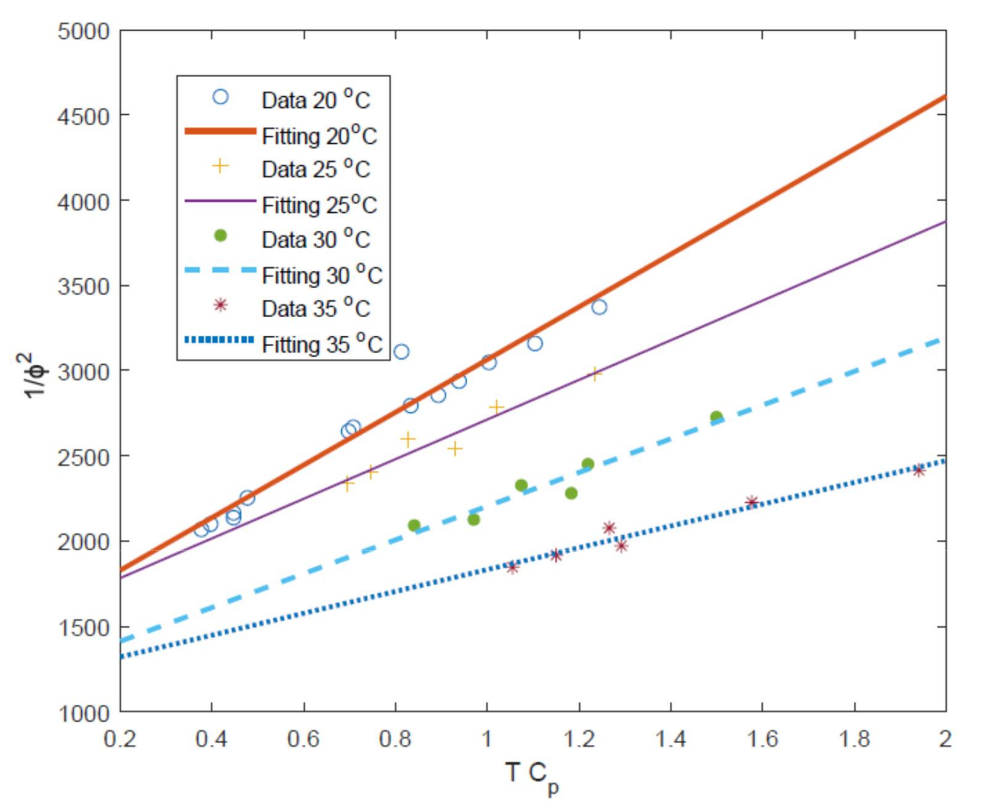
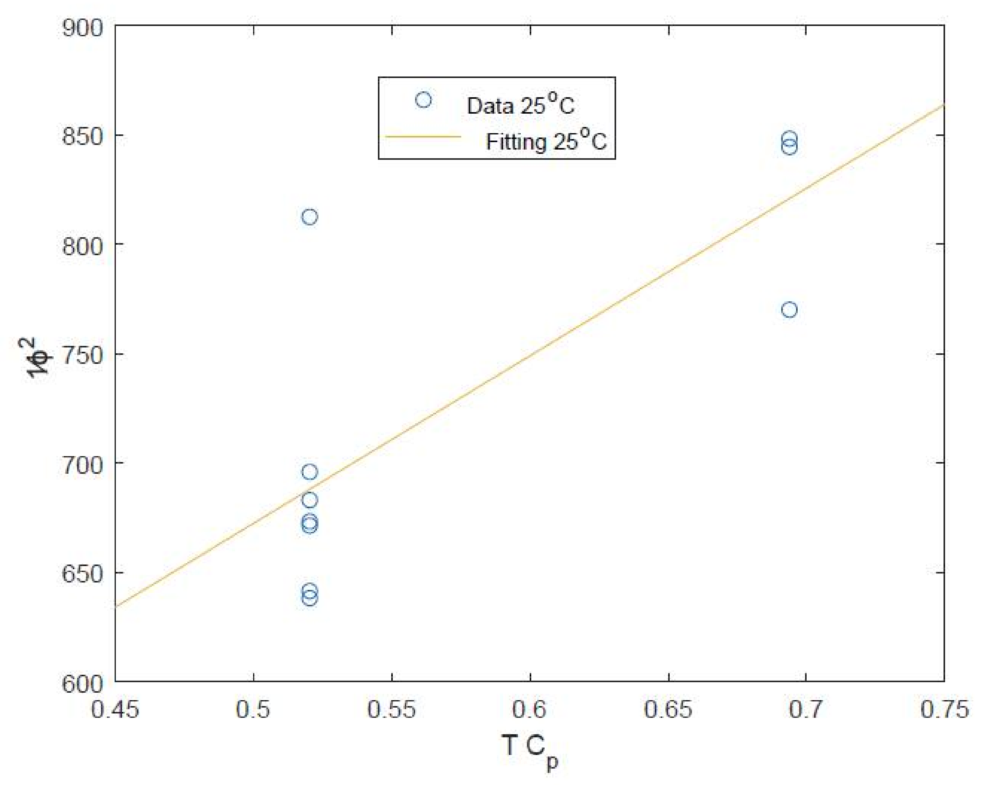
3.1. Determination of Pressure Coefficient b

Since the brine outlet pressures are not provided the above references, alternative methods must be used to estimate $b$.

Although the study of Avlonitis et al. [29] does not give a value of the friction coefficient $k_{fb}$, the value for this coefficient is given by the study of Senthilmurugan et al. as $2.5008\times {10}^8 m^{-2}$ [21]. This value is used together with the temperature and feed concentration from a selected feed condition from the 32 data points of Avlonitis et al., in this case 20 °C and 35 g/L are used together with Equations (35) and (19) to give the value of coefficient $b$.

For the Saehan module, the study of Mane et al. provides a value of the friction coefficient $k_{fb}=5.18\times {10}^{10}{m}^{-2}$ [23]. However, using this value leads to a calculated pressure drop which is much greater than the maximum pressure drop specified by the manufacturer for similar modules [40]. For this reason, the $b$ value is estimated for this case using the maximum pressure drop and the highest tested flow rate in Equation (20).

The estimated values of b are in this way given in

Table 2. Estimated and fitted parameters for case study of spiral wound membrane modules.

Spiral Wound Module	FilmTec FT30	Saehan RE4040-SR
$b\left({\mathrm{atm}\mathrm{m}}^{-4}{\mathrm{s}}^{-1}\right)$	$2.9760\times {10}^3$	$1.0126\times {10}^3$
$T_0\left(\mathrm{K}\right)$	$293.15$	$298.15$
$A_{\mathrm{w}0}\left({\mathrm{m}\mathrm{atm}}^{-1}{\mathrm{s}}^{-1}\right)$	$2.5258\times {10}^{-7}$	$2.7550\times {10}^{-7}$
$B_{\mathrm{S}0}\left({\mathrm{m}\mathrm{s}}^{-1}\right)$	$4.0699\times {10}^{-8}$	$1.7062\times {10}^{-8}$
$E_{\mathrm{A}}\left({\mathrm{J}\mathrm{mol}}^{-1}\right)$	$1.4192\times {10}^4$
$E_B$ $\left(\mathrm{J}{\mathrm{mol}}^{-1}\right)$	$4.2116\times {10}^4$
$B_{\left({\mathrm{H}}_3{\mathrm{BO}}_3\right)0}\left({\mathrm{m}\mathrm{s}}^{-1}\right)$		$5.4306\times {10}^{-7}$
$B_{\left({\mathrm{H}}_2{\mathrm{BO}}_3{}^{-}\right)0}\left({\mathrm{m}\mathrm{s}}^{-1}\right)$		$5.3760\times {10}^{-8}$
$A$	$-1.2604$	$5.619$
$B$	$0.35923$
$C$	$0.65885$	$0.5641$
$D$	$0.86483$

.

3.2. Determination of Water and Salt Transport Coefficients

As mentioned in Section 2.2 the values of water and salt transport coefficients can be determined by plotting $1/{\varphi }^2$ against $T{C}_{\mathrm{p}}$. In the study of Sundaramoorthy et al. a single value of these parameters ($A_{\mathrm{w}}$ and $B_{\mathrm{S}}$) is found to be sufficient for all the temperatures used when considering the removal of chlorophenol [30,31]. However, for the desalination of seawater, it is shown in Figure 3 that a separate linear fitting is required for each temperature, each giving different values of $A_{\mathrm{w}}$ and $B_{\mathrm{S}}$.

The data of Mane et al. is used for the fitting of $A_w$ and $B_S$ for the Saehan module (see Figure 4) although this is only a relatively small sample size using 10 out of the 15 data points available. Furthermore, this data set is also measured in a relatively narrow range of conditions including feed flow rates of 2.27 to 4 ${\mathrm{m}}^3{\mathrm{day}}^{-1}$ and salt rejection in the very narrow range of 99.6 to 99.7 % [23]. This is perhaps due to the study of Mane et al. focusing on boron recovery at different conditions [23]. Despite these limited data, it is still possible to estimate the values of water and salt coefficients with fitted values given in Table 2.

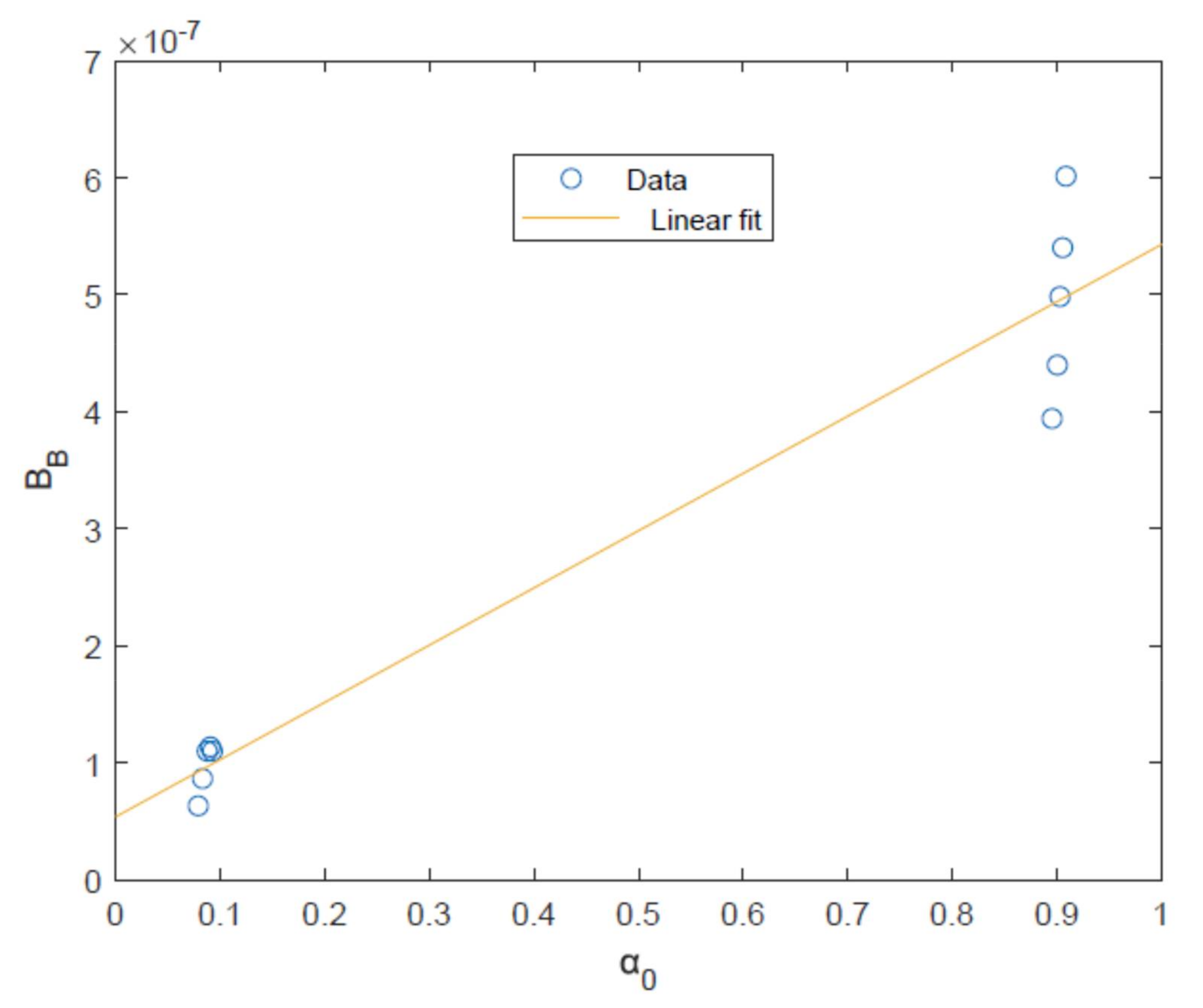
3.3. Determination of Boron Transport Coefficients

Since the data regarding boron are not available in the data of Avlonitis et al. [29] for the FilmTec module, parameters are fitted here only for the Saehan module based on the data of Mane et al. [23].

This is possible through plotting $B_B$ (calculated using Equation (33)) against ${\alpha }_0$ (calculated using Equation (30)) giving the plot and linear fit shown in Figure 5. The gradient and intercept of this linear fit are used to calculate $B_{\left(H_{3}B{O}_3\right)0}$ and $B_{\left(H_{2}B{O}_3{}^{-}\right)0}$ as given in Table 2.

3.4. Determination of Mass Transfer Correlation Coefficients

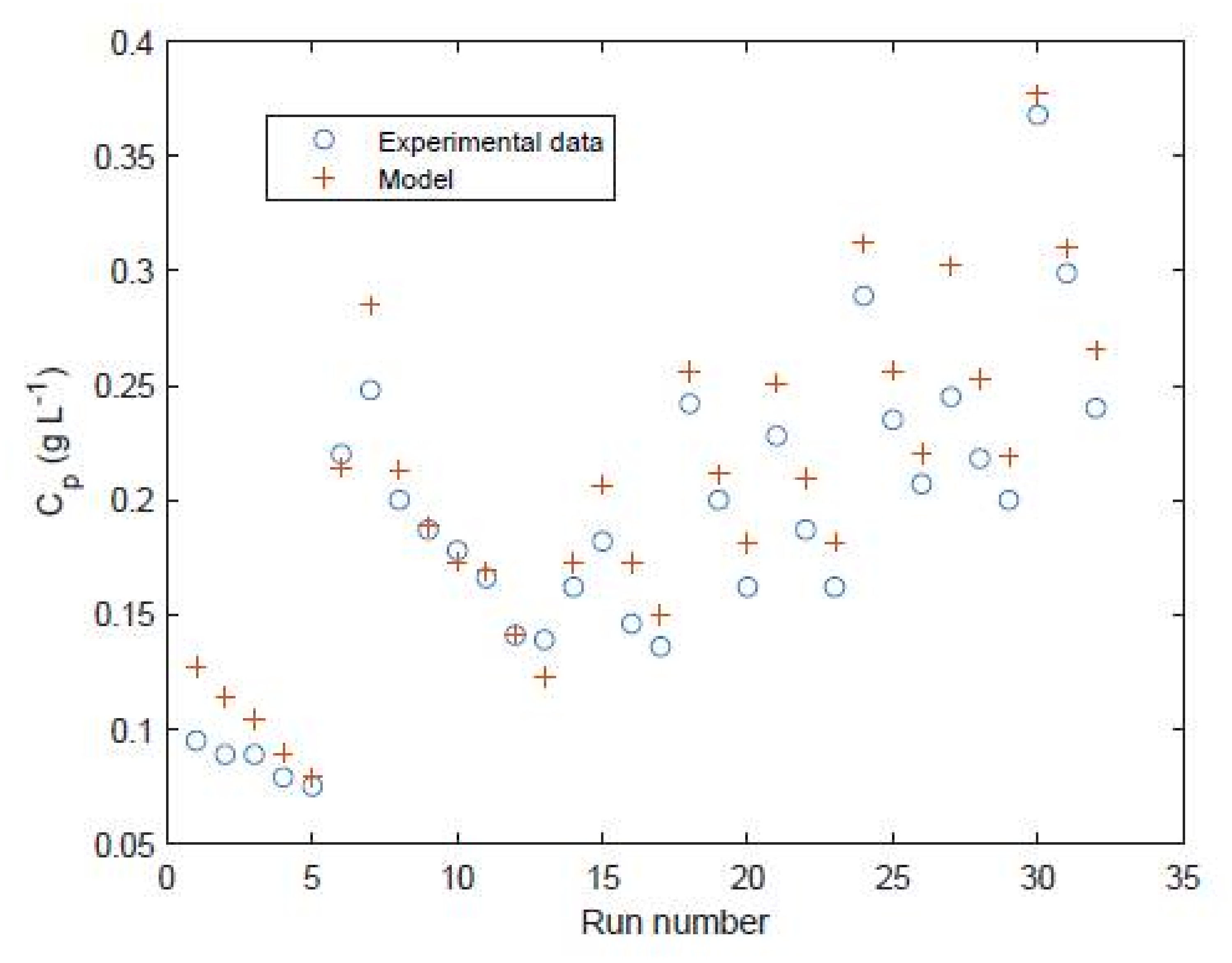
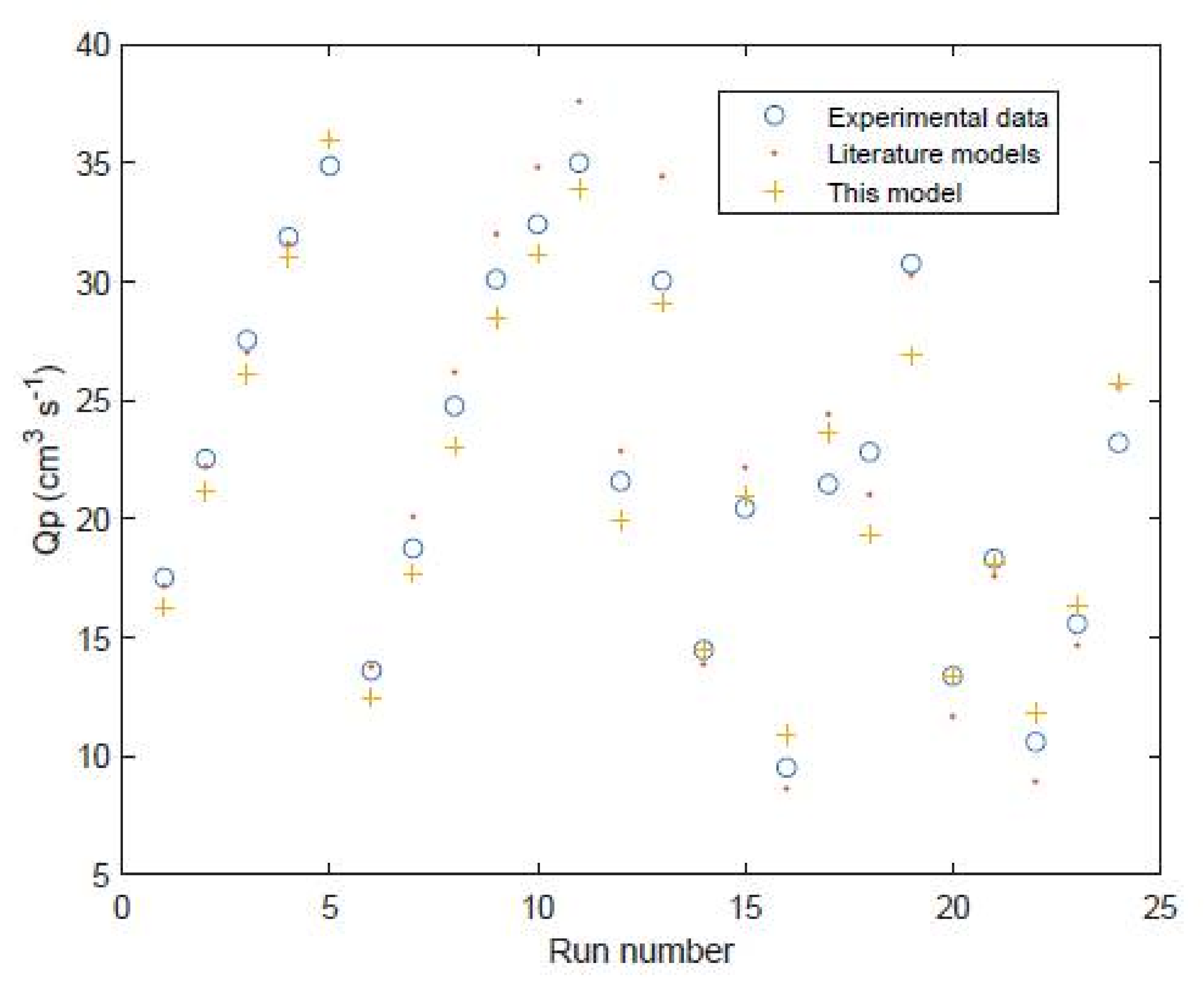
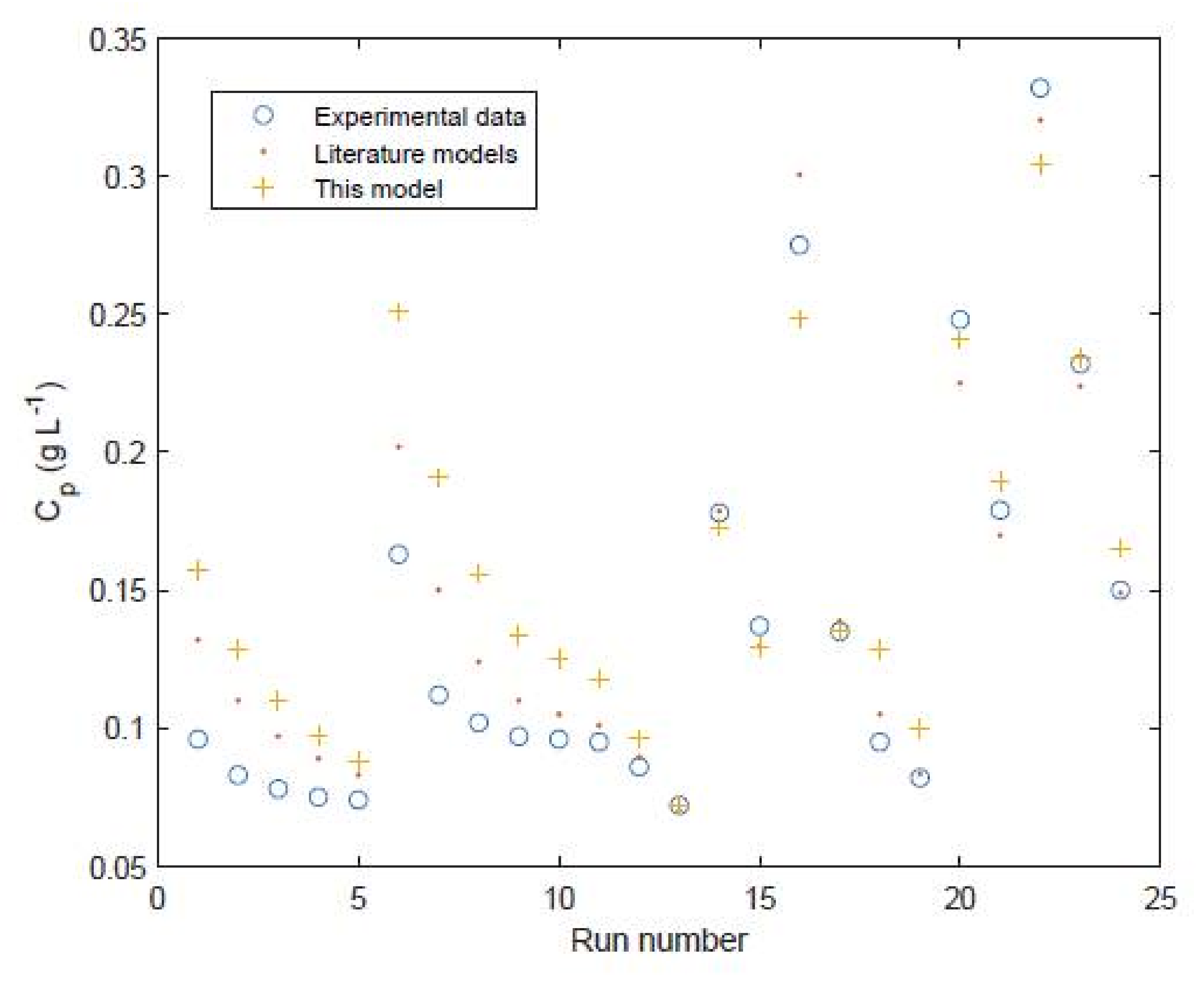
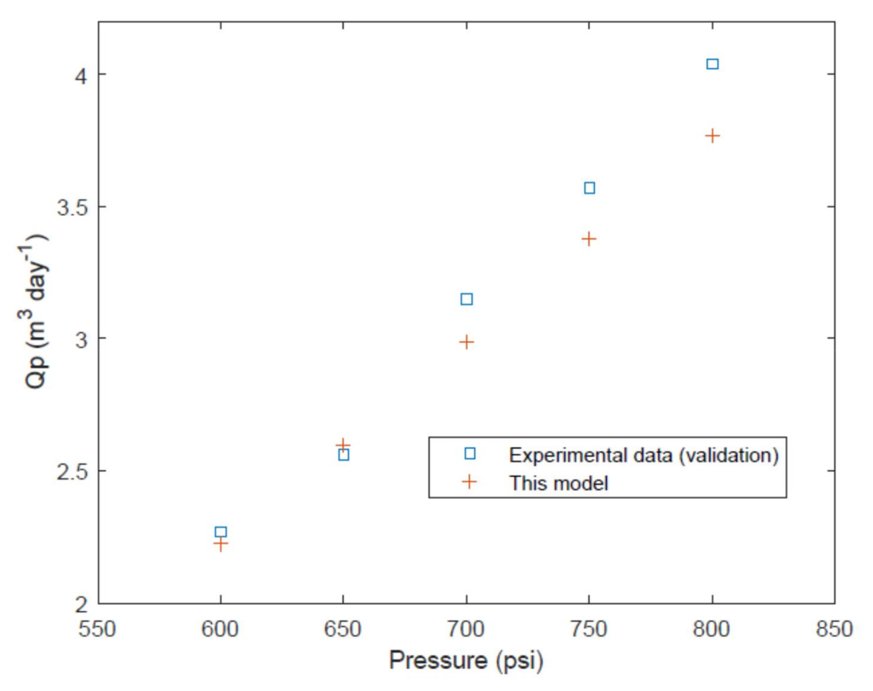
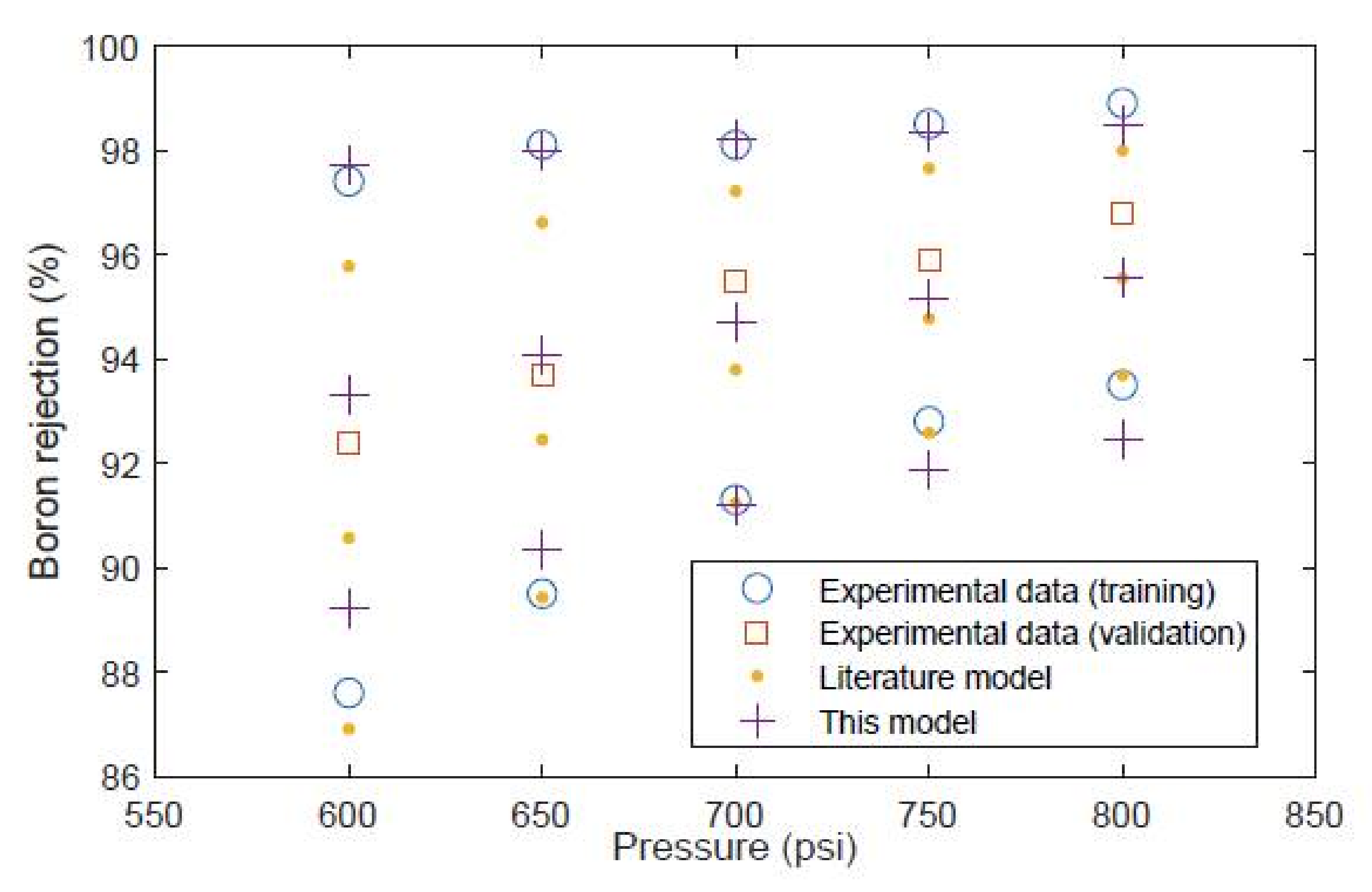
The value of the Sherwood number can be calculated for each experimental point. If both brine inlet and outlet data are available then the mass transfer coefficient and Sherwood number can be calculated for both points. However, in this case since the outlet pressures are not given in the case study references, only the inlet conditions are used to estimate mass transfer correlations:

$$k_{\mathrm{i}}=\frac{J_{\mathrm{Wi}}}{\ln \left[\left(\frac{J_{\mathrm{Wi}}}{B_{\mathrm{S}}}\right)\left(\frac{C_{\mathrm{p}}}{C_{\mathrm{i}}-C_{\mathrm{p}}}\right)\right]}$$

(42)

$$s{h}_{\mathrm{i}}=\frac{k_{\mathrm{i}}{D}_{\mathrm{i}}}{d_{\mathrm{e}}}$$

(43)

These values can be calculated for the two case studies considered here which can be used to fit values of $A$, $B$, $C,$ and $D$ in Equation (34). In principle, all four of these parameters can be fitted simultaneously using linear fitting, but some of these may be statistically insignificant, in particular for the Saehan membrane data which are based on 10 data points [23] all with very similar salt rejection and with the same value of $Sc$ at the inlet. For this reason initially $A$, $B,$ and $C$ were fitted simultaneously. However, when used in the prediction code, this sometimes led to erroneous calculations of $C_p=C_i$; perhaps because the correlation is overfitted to a narrow range of conditions. Hence, a simpler expression is tested using either $A$ and $B$ or $A$ and $C$. In other words, trying to fit a linear relation between either $\ln \left(sh\right)$ and $\ln \left(R{e}_{\mathrm{f}}\right)$ or $\ln \left(sh\right)$ and $\ln \left(R{e}_{\mathrm{p}}\right)$ and in this case $\ln \left(R{e}_{\mathrm{p}}\right)$ was found to more statistically significant; the values of $A$ and $C$ are given in Table 2.

For the FilmTec membrane module a larger set of data with 32 data points [29] was used to fit all four parameters as given in Table 2.

4. Model Validation

To show the prediction accuracy of the analytical model proposed here the model was tested both with the training set data and also data and conditions other than the training data.

For the FilmTec module the data from Table 2 is used in the model to predict the performance for the 32 data points used for training. The model is shown to predict reasonably well the permeate flow rate (Figure 6) and permeate salt concentration (Figure 7).

Furthermore this model is then validated against two sets of experimental data and associated models from the literature (11 data points and analytical model results from Table 2 in the study of Avlonitis et al. [29] and 13 data points and numerical model results from Table 9 in the study of Senthilmurugan et al. [21]) which are labelled as run numbers 1–11 and run numbers 12–24 in Figure 8 and Figure 9. This validation shows that the proposed model is reasonably accurate for all of the data points. The only exception is the permeate concentrations for run numbers 1–11 which are overpredicted by the model. The model of Avlonitis et al. is shown to predict these values slightly more accurately [29]. This is presumably because the model of Avlonitis et al. has been trained/fitted using a wider range of data which are not covered inside the training set of 32 data points [29]. The proposed model is shown to give similar accuracy compared to the numerical model of Senthilmurugan et al. [21] in most of the run numbers 12–24. The overall accuracy of the proposed model is 6.3% for water permeation and 24.7% for permeate concentration. However, the accuracy of the model for runs 12–24 is 7.2% for water permeation and 8.9% for permeate concentration. If the model was retrained using data from run numbers 1–11 these errors in the permeate concentration could potentially be reduced. The more complex numerical model of Senthilmurugan et al. gives an accuracy for runs 12–24 of 8.8% for water permeation and 4.5% for permeate concentration.

Run numbers 1–11 show the experimental and model results from Avlonitis et al. [29] and run numbers 12–24 show the experimental and model results from Senthilmurugan et al. [21].

For the Saehan module the data from Table 2 is used in the model to predict the performance for the 5 data points used for testing/validation. The model is shown to predict reasonably well the permeate flow rate (Figure 10).

Furthermore, the boron rejection predicted by this model is compared against the experimental and model predictions of Mane et al. [23], as shown in Figure 11. In this Figure, the 10 data points denoted by empty circles/rings are those which were used for training and the squares are the data points which were used for testing. In this Figure, the literature model results are those given in the study of Mane et al. which were generated using a complex finite elements numerical model [23]. That model uses the boric acid $\left({\mathrm{H}}_3{\mathrm{BO}}_3\right)$ and borate ion $\left({\mathrm{H}}_2{\mathrm{BO}}_3{}^{-}\right)$ transport coefficients given by Hyung and Kim [24], while the proposed model uses coefficients which are fitted to the experimental data of Mane et al. [23]. It can be seen that the model of Mane et al. fits well to the values at lower rejection data points (these values are for pH 7.5) but underpredicts the values at higher rejection (with pH at 8.5 and 9.5). Meanwhile, the proposed model gives a reasonably accurate prediction for all data points, except for some slight over- and underprediction at the lower pH values. For the testing data in Figure 11, the proposed model gives an absolute average error of 0.82% while the model of Mane et al. gives an absolute average error of 1.44%.

5. Conclusions

An analytical model is proposed in this study for simultaneously predicting the removal of both salt and boron from seawater through reverse osmosis using spiral wound desalination membrane modules. This model and the fitting procedure is an extension of the methods proposed by Sundaramoorthy et al. for the removal of organic solutes [30,31] which is modified and extended to predict the removal of both salt and boron from seawater.

The fitting procedure proposed here is sequential, starting with the prediction of a pressure drop coefficient, followed by the fitting of water and salt transport coefficients. Subsequently the boron transport coefficients and the mass transfer correlation coefficients can be fitted independently of each other. In all of these steps it is shown that the parameters can be obtained through linear fitting using experimental values and calculated parameters from previous steps. Hence, this approach offers a very simple method for obtaining all the parameters needed to build the predictive model.

The analytical model equations can be solved by following the steps given in Section 2.3 which offers a much simpler method for simulation of separation performance compared with the more complex numerical finite-difference type models which require solving much larger numbers of equations and more computational effort. A basic comparison of the CPU time required to simulate three modules 1000 times (optimization will typically require simulation of configurations at least 1000 times, in some cases much more) shows that the proposed analytical model required 7.3 s while a numerical model with 100 discrete points required 4 min 21.2 s using an i7 3.30 GHz intel computer.

Although the proposed model is simpler than numerical finite-difference type models it is shown to give similar accuracy when comparing the predicted outlet permeate flow rate, salt, and boron rejection. This type of model should be appropriate for the design and optimization of multistage desalination systems due to its simplicity and low computational requirements.

References

1. WHO. Guidelines for Drinking-Water Quality: Fourth Edition Incorporating the First Addendum; World Health Organization: Geneva, Switzerland, 2017; Licence: CC BY-NC-SA 3.0 IGO. [Google Scholar]
2. Najid, N.; Kouzbour, S.; Ruiz-Garcia, A.; Fellaou, S.; Gourich, B.; Stiriba, Y. Comparison analysis of different technologies for the removal of boron from seawater: A review. J. Environ. Chem. Eng. 2021, 9, 105133. [Google Scholar] [CrossRef]
3. Hilal, N.; Kim, G.J.; Somerfield, C. Boron removal from saline water: A comprehensive review. Desalination 2011, 273, 23–35. [Google Scholar] [CrossRef]
4. Redondo, J.; Busch, M.; De Witte, J.-P. Boron removal from seawater using filmtech high rejection SWRO membranes. Desalination 2003, 156, 229–238. [Google Scholar] [CrossRef]
5. Koseoglu, H.; Kabay, N.; Yuksel, M.; Sarp, S.; Arar, O.; Kitis, M. Boron removal from seawater using high rejection SWRO membranes—Impact of pH, feed concentration, pressure, and cross-flow velocity. Desalination 2008, 227, 253–263. [Google Scholar] [CrossRef]
6. Ali, Z.; Sunbul, Y.A.; Pacheco, F.; Ogieglo, W.; Wang, Y.; Genduso, G.; Pinnau, I. Defect-free highly selective polyamide thin-film composite membranes for desalination and boron removal. J. Membr. Sci. 2019, 578, 85–94. [Google Scholar] [CrossRef]
7. Li, Y.; Wang, S.; Song, X.; Zhou, Y.; Shen, H.; Cao, X.; Zhang, P.; Gao, C. High boron removal polyamide reverse osmosis membranes by swelling induced embedding of a sulfonyl molecular plug. J. Membr. Sci. 2020, 597, 117716. [Google Scholar] [CrossRef]
8. Haidari, A.H.; Heijman, S.G.J.; van der Meer, W.G.J. Optimal design of spacers in reverse osmosis. Sep. Purif. Technol. 2018, 192, 441–456. [Google Scholar] [CrossRef]
9. Ruiz-Garcia, A.; Nuez, I. Performance assessment of SWRO spiral-wound membrane modules with different feed spacer dimensions. Processes 2020, 8, 692. [Google Scholar] [CrossRef]
10. Tu, K.L.; Nghiem, L.D.; Chivas, A.R. Boron removal by reverse osmosis membranes in seawater desalination applications. Sep. Purif. Technol. 2010, 75, 87–101. [Google Scholar] [CrossRef]
11. Ban, S.-H.; Im, S.-J.; Cho, J.; Jang, A. Comparative performance of FO-RO hybrid and two-pass SWRO desalination processes: Boron removal. Desalination 2019, 471, 114114. [Google Scholar] [CrossRef]
12. Jung, B.; Kim, C.Y.; Jiao, S.; Rao, U.; Dudchenko, V.; Tester, J.; Jassby, D. Enhancing boron rejection on electrically conducting reverse osmosis membranes through local electrochemical pH modification. Desalination 2020, 476, 114212. [Google Scholar] [CrossRef]
13. Landsman, M.R.; Lawler, D.F.; Katz, L.E. Application of electrodialysis pretreatment to enhance boron removal and reduce fouling during desalination by nanofiltration/reverse osmosis. Desalination 2020, 491, 114563. [Google Scholar] [CrossRef]
14. Ruiz-Garcia, A.; Nuez, I. Performance evaluation and boron rejection in a SWRO system under variable operating conditions. Comput. Chem. Eng. 2021, 153, 107441. [Google Scholar] [CrossRef]
15. Al-Obaidi, M.A. Evaluation of chlorophenol removal from wastewater using multi-stage spiral-wound reverse osmosis process via simulation. Comput. Chem. Eng. 2019, 130, 106522. [Google Scholar] [CrossRef]
16. Al-Obaidi, M.A.; Kara-Zaitri, C.; Mujtaba, I.M. Performance evaluation of multi-stage reverse osmosis process with permeate and retentate recycling strategy for the removal of chlorophenol from wastewater. Comput. Chem. Eng. 2019, 121, 12–26. [Google Scholar] [CrossRef] [Green Version]
17. Alsarayreh, A.A.; Al-Obaidi, M.A.; Al-Hroub, A.M.; Patel, R.; Mujtaba, I.M. Performance evaluation of reverse osmosis brackish water desalination plant with different recycled ratios of retentate. Comput. Chem. Eng. 2020, 135, 106729. [Google Scholar] [CrossRef]
18. Alsarayreh, A.A.; Al-Obaidi, M.A.; Patel, R.; Mujtaba, I.M. Scope and limitations of modelling, simulation, and optimisation of a spiral wound reverse osmosis process-based water desalination. Processes 2020, 8, 573. [Google Scholar] [CrossRef]
19. Joseph, A.; Damodaran, V. Dynamic simulation of the reverse osmosis process for seawater using labview and an analysis of the process performance. Comput. Chem. Eng. 2019, 121, 294–305. [Google Scholar] [CrossRef]
20. Ben Boudinar, M.; Hanbury, W.T.; Avlonitis, S. Numerical simulation and optimisation of spiral-wound modules. Desalination 1992, 86, 273–290. [Google Scholar] [CrossRef]
21. Senthilmurugan, S.; Ahluwalia, A.; Gupta, S.K. Modeling of a spiral-wound module and estimation of model parameters using numerical techniques. Desalination 2005, 173, 269–286. [Google Scholar] [CrossRef]
22. Geraldes, V.; Periera, N.E.; de Pinho, M.N. Simulation and optimization of medium-sized seawater reverse osmosis processes with spiral-wound modules. Ind. Eng. Chem. Res. 2005, 44, 1897–1905. [Google Scholar] [CrossRef]
23. Mane, P.P.; Park, P.K.; Hyung, H.; Brown, J.C.; Kim, J.H. Modeling boron rejection in pilot- and full-scale reverse osmosis desalination processes. J. Membr. Sci. 2009, 338, 119–127. [Google Scholar] [CrossRef]
24. Hyung, H.; Kim, J.H. A mechanistic study on boron rejection by sea water reverse osmosis membranes. J. Membr. Sci. 2006, 286, 269–278. [Google Scholar] [CrossRef]
25. Ruiz-Garcia, A.; Leon, F.A.; Ramos-Martin, A. Different boron rejection behavior in two RO membranes installed in the same full-scale SWRO desalination plant. Desalination 2019, 449, 131–138. [Google Scholar] [CrossRef]
26. Sassi, S.M.; Mujtaba, I.M. MINLP based superstructure optimization for boron removal during desalination by reverse osmosis. J. Membr. Sci. 2013, 440, 269–278. [Google Scholar] [CrossRef]
27. Taniguchi, M.; Kurihara, M.; Kimura, S. Boron reduction performance of reverse osmosis seawater desalination process. J. Membr. Sci. 2001, 183, 259–267. [Google Scholar] [CrossRef]
28. Du, Y.; Liu, Y.; Zhang, S.; Xu, Y. Optimization of seawater reverse osmosis desalination networks with permeate split design considering boron removal. Ind. Eng. Chem. Res. 2016, 55, 12860–12879. [Google Scholar] [CrossRef]
29. Avlonitis, S.; Hanbury, W.T.; Ben Boudinar, M. Spiral wound modules performance an analytical solution: Part II. Desalination 1993, 89, 227–246. [Google Scholar] [CrossRef]
30. Sundaramoorthy, S.; Srinivasan, G.; Murthy, D.V.R. An analytical model for spiral wound reverse osmosis membrane modules: Part I—Model development and parameter estimation. Desalination 2011, 280, 403–411. [Google Scholar] [CrossRef]
31. Sundaramoorthy, S.; Srinivasan, G.; Murthy, D.V.R. An analytical model for spiral wound reverse osmosis membrane modules: Part II—Experimental validation. Desalination 2011, 277, 257–264. [Google Scholar] [CrossRef]
32. Srinivasan, G.; Sundaramoorthy, S.; Murthy, D.V.R. Validation of an analytical model for spiral wound reverse osmosis membrane module using experimental data on the removal of dimethlyphenol. Desalination 2011, 281, 199–208. [Google Scholar] [CrossRef]
33. Fraidenraich, N.; de Castro Vilela, O.; dos Santos Viana, M.; Gordon, J.M. Improved analytic modeling and experimental validation for brackish-water reverse-osmosis desalination. Desalination 2016, 380, 60–65. [Google Scholar] [CrossRef]
34. Al-Obaidi, M.A.; Kara-Zaitri, C.; Mujtaba, I.M. Removal of phenol from wastewater using spiral-wound reverse osmosis process: Model development based on experiment and simulation. J. Water Process Eng. 2017, 18, 20–28. [Google Scholar] [CrossRef] [Green Version]
35. Al-Obaidi, M.A.; Li, J.-P.; Alsadaie, S.; Kara-Zaitri, C.; Mujtaba, I.M. Modelling and optimisation of a multistage reverse osmosis processes with permeate reprocessing and recycling for the removal of N-nitrosodimethylamine from wastewater using species conserving genetic algorithms. Chem. Eng. J. 2018, 35, 824–834. [Google Scholar] [CrossRef] [Green Version]
36. Koutsou, C.P.; Yiantsios, S.G.; Karabelas, A.J. Direct numerical simulation of flow in spacer-filled channels: Effect of spacer geometrical characteristics. J. Membr. Sci. 2007, 291, 53–69. [Google Scholar] [CrossRef]
37. Mehdizadeh, H.; Dickson, J.M.; Eriksson, P.K. Temperature effects on the performance of thin-film composite, aromatic polyamide membranes. Ind. Eng. Chem. Res. 1989, 28, 814–824. [Google Scholar] [CrossRef]
38. Nir, O.; Lahav, O. Coupling mass transport and chemical equilibrium models for improving the prediction of SWRO permeate boron concentrations. Desalination 2013, 310, 87–92. [Google Scholar] [CrossRef]
39. Koroneos, C.; Dompros, A.; Roumbas, G. Renewable energy driven desalination systems modelling. J. Clean. Prod. 2007, 15, 449–464. [Google Scholar] [CrossRef]
40. Saehan Technical Manual. Available online: http://www.csmfilter.co.kr/searchfile/file/Tech_manual.pdf (accessed on 11 May 2021).
Figure 1. Spiral wound membrane geometry (unwound diagram).
Sustainability 13 08999 g001
Figure 2. Parameter estimation steps for a spiral wound reverse osmosis desalination membrane.
Sustainability 13 08999 g002
Figure 3. Plot of the 1 / ϕ 2 against T C p with linear fitting against the data of Avlonitis et al. [29] using the calculated value of b from Table 2.
Sustainability 13 08999 g003
Figure 4. Plot of the 1 / ϕ 2 against T C p with linear fitting against the data of Mane et al. [23] using the calculated value of b from Table 2.
Sustainability 13 08999 g004
Figure 5. Plot of B B (calculated using experimental data [23] and fitted parameters b , A w , and B s ) against α 0 together with linear fit.
Sustainability 13 08999 g005
Figure 6. Permeate flow rate of FilmTec module comparison of experimental values [29] against model predictions for the 32 data points used to train the model.
Sustainability 13 08999 g006
Figure 7. Permeate salt concentration of FilmTec module comparison of experimental values [29] against model predictions for the 32 data points used to train the model.
Sustainability 13 08999 g007
Figure 8. Permeate flow rate of FilmTec module comparison of experimental values [4,11] against model predictions for 24 different data points for testing/validation.
Sustainability 13 08999 g008
Figure 9. Permeate salt concentration of FilmTec module comparison of experimental values [4,11] against model predictions for 24 different data points for testing/validation. Run numbers 1–11 show the experimental and model results from Avlonitis et al. [29] and run numbers 12–24 show the experimental and model results from Senthilmurugan et al. [21].
Sustainability 13 08999 g009
Figure 10. Permeate volume flow rate. A comparison of experimental data [23] and model predictions.
Sustainability 13 08999 g010
Figure 11. Boron rejection for the Saehan module. A comparison of experimental data [23] and model predictions.
Sustainability 13 08999 g011