Abstract
Since thermal power generation is still one of the main sources of carbon emissions in China, the economic benefits and productivity of the thermal power generation industry have been seriously affected in recent years with the increasingly strict environmental regulations and restrictions on carbon emissions, as well as by the sharp fluctuations of coal prices. Therefore, it has been an important issue to improve the productivity performance of the thermal power industry. Due to the regional heterogeneity among different regions of China, we introduced a meta-frontier framework into the energy cost productivity model to develop a meta-energy cost productivity model. The energy cost gap between the group-specific and meta-frontiers was also utilized to assess the convergence rate of the group-specific frontier to the meta-frontier. The estimated results present that the energy cost efficiency of the eastern region outperformed that of the other two regions, and the cost Malmquist (CM) productivity of these three regions all showed positive growth, in which the progress of allocative efficiency and price effect were the main driving factors. Additionally, the central and western regions displayed the convergence of group-specific CM productivity towards the meta-frontier.
1. Introduction
Global warming caused by CO2 emissions has caused a certain negative impact on the human living environment. The Paris Agreement requires that the global average temperature rise in this century should not exceed 2 °C and that the global temperature rise should be limited to 1.5 °C [1]. For this reason, it is necessary to phase out carbon emissions from fossil fuels and other anthropogenic sources [2]. The global demand for electricity will continue to increase, and its share of final energy consumption is also expected to rise [3]. The production and supply of electric power and heat power account for more than 40 percent of world’s CO2 emissions related to energy, because fossil fuels are still the major factor in thermal power generation. Coal, in particular, has long been the most important fuel for the thermal power industry. In terms of a report released by the IPCC, thermal power generation must be gradually stopped by 2050 to realize the global temperature rise target [4]. Especially in the past few decades in China, thermal power has been the main form of electronic generation, which has generated over 80% of the total power during this process. Nevertheless, since the “separate power plants from the grid” and “yardstick power price” came out and have been applied by certain sectors, the electricity price has not kept pace with the rise in market-oriented coal prices [5]. Moreover, the cost of coal and labor occupies a large proportion of the total cost of the thermal power industry—the fluctuations of coal prices and the increases in labor costs had great impacts on the profit level and cost control of coal-fired power enterprises over the sample period, as shown in Figure 1 and Figure 2. In recent years, the performance of the thermal power plants has declined. Therefore, it is extremely essential to alleviate and turn around the decline in performance [6].
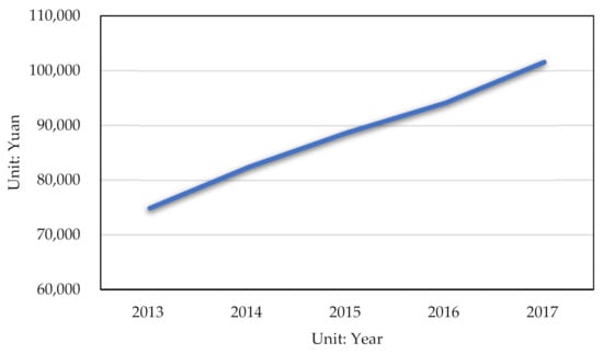
Figure 1.
The average wage of the thermal power industry from 2013 to 2017.
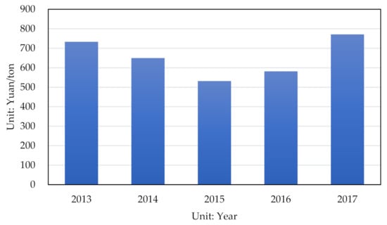
Figure 2.
The changes of standard coal price (standard coal, also known as coal equivalent, is a unified unit of energy that converts different kinds of energy with different caloric content into a standard content according to their different caloric content) from 2013 to 2017.
Two major methods are widely utilized in related studies to improve the performance of the Chinese thermal power industry. Under certain power demands, the first one is to directly increase the revenue of sales by raising the electricity price [7,8,9], and the second one is to take several actions to reduce production and management costs through indirectly improving the cost efficiency (CE) of each company [10,11,12,13,14]. Since 2005, the central governmental sector has enforced the policy of “coal–electricity price linkage” many times. The effect of economic benefits was not obvious, and the power shortage occurred frequently [15]. However, by improving technical progress and optimizing allocation of resources, power plants can offset the undesirable impact of variations in fuel price and promote production efficiency to some extent, which highlights the importance of improving CE. Moreover, in terms of the reports published by the International Energy Agency (IEA) in 2018, approximately 58.6% of carbon dioxide emissions came from the thermal power industry. Hence, both price factors and CO2 emissions must be considered when measuring the CE of the thermal power industry, which is related to the data development analysis (DEA) method.
Charnes et al. [16] first came up with the concept of a non-parametric DEA approach, which has been utilized many times in this field. The main advantage of this method is that it allows researchers to ignore the functional form and dimension between the inputs and outputs. A great many achievements have been made with this tool, especially its application in the thermal power industry. Further, under the assumption of VRS and CRS, Färe et al. [17] measured the technical efficiency (TE), scale efficiency (SE), and input congestion of several power companies in Illinois by using the DEA approach. Applying the same method, Olatubi and Dismukes [18] attempted to measure the opportunities of CE for American coal-fired power plants. However, these papers only considered the static case of efficiency evaluation.
On the basis of the input-oriented distance functions proposed by Shephard [19], Färe et al. [20] came up with a new Malmquist productivity index to estimate the variations of efficiency through a dynamic method. This indicator can be divided into the changes of TE and frontier technology, which was used to analyze growth rate of productivity in Illinois coal-fired steam electric companies from 1975 to 1981. Yunos and Hawdon [21] estimated the economic performance and development of Malaysian electricity generation and made the comparison with other countries at the similar development level. Also, over the period 1969–1999, Abbott [22] measured the change of productivity of the electricity supply industry in Australia, and he analyzed the impacts of reformation on efficiency through the DEA method. Thereafter, Chung et al. [23] first came up with the Malmquist–Luenberger (ML) productivity index. In terms of the new indicator, Kumar [24] then took the environmental factors into account and assessed the productivity growth of the thermal power industry for developed and developing countries.
With the continuous progress and improvement of DEA method, an increasing number of Chinese researchers have used various models within the DEA field to assess the environmental and energy efficiency of Chinese thermal power plants. Lam and Shiu [25] applied the traditional non-parametric DEA model to assess the efficiency of plants related to the thermal power generation in a study that mainly concentrated on the TE. They figured out that power industries in the eastern coastal China had the best performance in terms of technology progress. However, the undesirable outputs were not introduced into the DEA framework in this study. Yu et al. [26] utilized the factor analysis and constructed a two stage DEA model to estimate the cost and quality performance of electricity distribution enterprises related to thermal power in the UK. Over the period 2003–2006, Kaneko et al. [27] measured the changes of marginal abatement costs, which decreased by 50% in the coal-fired power industry. Assaf et al. [28] applied the Bayesian frontier model to analyze the CE of power generation companies over the period 1976–2003 in Japan. On the basis of a meta-frontier non-radial DEA method, Zhang et al. [29] estimated the energy and CO2 emissions performance in thermal power generation in South Korea. With a total factor productivity framework, Chang and Hu [30] came up with total factor energy productivity change indicator according to the traditional total factor Luenberger productivity index to estimate the changes of energy productivity in Chinese regions. Wang et al. [8] considered the price factor and used the cost ML indicator to calculate the provincial CE of the thermal power industry in China. Bi et al. [31] divided China into four regions, and then calculated total-factor energy efficiency of Chinese power generation sectors by introducing an input-oriented SBM method. Constructing a new model with the bootstrap method and a directional distance function, Duan et al. [32] evaluated the environmental and energy efficiency of thermal power plants, and this study discovered that improvement of technology is the major strength in promoting overall efficiency. Wang et al. [9] utilized the DEA method to calculate the efficiency of abatement and environment in the Chinese thermal power industry on the basis of a material balance approach. Yan et al. [33] applied the SBM approach to assess the scores of operational efficiency in the Chinese thermal power sector of provinces.
Though the research mentioned above estimated the energy efficiency and productivity growth of the thermal power industry, most of them did not take cost factors into consideration in the evaluation model. Therefore, in our study, we constructed a cost Malmquist productivity index (CMPI) to take into consideration the inputs’ price factors and capture the effect of allocative distortions in inputs. Although a few studies [8,9,10] have assessed the CE and productivity of the thermal power industry through various perspectives of related productivity indices, none of them have taken the heterogeneity into account due to the differences in production technology and the different environments among provinces in different regions. The view was expressed by Huang et al. [34] that due to the heterogeneity in production technology among these three regions, it is appropriate to make comparisons of group-specific and meta-CMPI. We therefore extended the CMPI model in the framework of a meta-frontier and introduced carbon emissions as one of outputs of the model. Meanwhile, we also combined this with the DEA approach to estimate the CE of the thermal power industry in 30 Chinese provinces. Compared to other methods, meta-CMPI and meta-CE can make the comparison of productivity and efficiency related to the subject of cost minimization. Furthermore, the CM gap is applied to assess the convergence or divergence of the group-specific CMPI toward the meta-CMPI.
The 30 tested provinces were divided into eastern, central, and western regions. The labor, auxiliary power consumption, installed capacity, and energy consumption were viewed as the inputs of production. Corresponding to the inputs, the input prices were average wage, electricity price, cost of generator, and standard coal price. The outputs were divided into two types: desirable and undesirable. The GDP support created by the power and power generation were viewed as the good outputs, and the CO2 emissions were used as the bad output. The meta-CMPI and DEA methods mentioned above were utilized to assess the CM productivity and CE of the thermal power industry from 2013 to 2017. The empirical results show that both the meta-CE and the group-specific CE of the eastern region outperformed that of the other two regions due to the contribution of allocative efficiency (AE). The CMPI of the three regions all presented a positive growth during the sample period, among which the optimization of price effect (PE) was the main driving factor. Except for the eastern region, the other two regions displayed the convergence of group-specific CMPI towards the meta-frontier CMPI. Only three provinces can be viewed as benchmarks in the BCG analysis. The specific interpretation of each abbreviation is presented in (Appendix A) Table A1.
The rest of the paper mainly consists of the following parts: Section 2 presents the construction process of CMPI. Section 3 displays the sources of data related to all variables in this study, and shows the analysis of estimated results from the CMPI. The conclusions and some policy implications are stated in the final section.
2. Materials and Methods
2.1. Group-Specific and Meta-Frontier Technology
Based on the panel data, there are j (j = 1, 2, …, J) production regions (group) of the thermal power industry and they set each province as a DMU. We assume that the jth region’s DMU utilize xt inputs ( to generate yt desirable outputs () and bt undesirable outputs () at the t period (t = 1, 2, …, T). The group-specific production technology can be defined as . The feature of is supposed to be bounded, closed, non-void, and convex. The input requirement sets can be used to represent the production technology, with the following isoquant:
We can apply the input distance function (DF) developed by Shephard [20] to express the as:
On the basis of a given output vector, the input DF can offer the maximum number of input vectors, and then a DMU can shrink this vector according to the upper limit. In this paper, the radial contractions were the main assumption for all adjustments of input variables. In the jth production group, we defined the group-specific TE, which is a subset constrained by meta-frontier technology as follows:
As for the meta-frontier technology, it can be defined as the envelope that contains all production techniques from J, i.e., which is different from the meta-framework of Pastor and Lovell [35] because it only contains the contemporaneous frontiers covering all periods. We defined the meta input requirement sets as: and its corresponding isoquant as follows:
Similar to the above group-specific DF, the meta-DF, and the TE can be constructed as:
Due to the different defining feature of two technologies, we found that , and then . We now introduced cost prices of inputs into the model and assumed that DMUs in the jth region seek to minimize production costs, and then define the group-specific cost function (CF) subject to as:
2.2. Cost Efficiency, Decompositions, and Efficiency Gap
Here, we show the formula to calculate the group-specific CE, namely the ratio of the CF to the actual cost:
where . If the , it indicates that this DMU is using an excess number of inputs to generate certain outputs, or that it is using an inappropriate combination of inputs at the current levels of input price, or both problems exist. The former leads to the reduction of TE, and the latter leads to a decrease in AE. The values of TE and AE are all less than or equal to 1. In terms of Equations (3) and (10), the AE of inputs can be stated as:
Therefore, the CE and its decompositions, TE and AE, are related to each other and are bound by the above restrictions:
The meta-CF and the meta-CE and its components are similarly defined as:
The cost gap, which can also be called the CE gap, is used to estimate the distance between the meta-CF and group-specific CF. Given the observed DMU produce output yt with input price wt at the period t, namely the ratio of group-specific CF to the meta-CF. The cost gap can be defined as:
Hence, according to the Equation (12), the cost gap can also be decomposed into the gap TE and AE as follows:
where is bounded by 1. If the > 1, it is implied that identical yt produced through the group-specific technology is more cost-effective than through the meta-technology. If the > 1, it signifies that the DMU can save certain usage of inputs when producing the identical outputs in case of the meta-technology. As for , it can assess the difference in the allocation of inputs over the current level of input prices between the group-specific and meta-technology. If the value of > 1, it implies that the group-specific AE outperforms the meta-AE, otherwise the group-specific AE is inferior to the meta-AE.
2.3. Cost Malmquist Productivity Index and Its Decompositions
Caves et al. [36] first came up with the original Malmquist productivity indicator, and then Färe et al. [37] developed this index to measure the productivity performance of the producer. Nevertheless, due to better or worse adjustment of the input mix with the current input prices, the indictor mentioned above cannot reflect the feature of the changes in AE. Thus, Maniadakis and Thanassoulis [38] first took the input cost and quantity DF into consideration, which came up with the CMPI. Its four components can capture changes in TE, AE, T, and PE.
Referring to the conventional CMPI proposed by Maniadakis and Thanassoulis [38], we constructed the CMPI at the period t as , and the index at the period t+1 is . Then, the group-specific CMPI can be defined as:
where the value of > 1 indicates that productivity growth otherwise indicates the decline of productivity. According to the formula listed above, the can also be stated as follows:
Assuming the constant returns to scale (CRS), all the group-specific decompositions are evaluated under this assumption. If the and > 1, this implies that cost efficiency (CE) and cost technology (CT) improve during the sample period, while the value < 1 implies regress. In terms of the Equation (10), the can be divided into the growth of TE and AE as below:
where the value of > 1, signifying progress, otherwise signifies regress.
Further, the can be divided into the growth of T and PE as:
where the is the variation of technology and reflects the variations of benchmark technology during the given period. The represents the residual variation in the CF, which mainly results from the change from wt to wt+1. If the > 1, this indicates a positive PE, while the < 1 denotes a negative PE.
In sum, we divided the group-specific CMPI from Maniadakis and Thanassoulis [38] into four components:
Including all group-specific frontiers for a given period of time, meta-frontier stands for the potentially best frontier technology over all groups. The construction of meta-CMPI and its decompositions is similar to that of group-specific CMPI (. Hence, the meta-CMPI and its decompositions are constructed as:
where the construction of each meta component is similarly defined as the Equation (17) by changing the subscript to the meta asterisk (*).
For the sake of reflecting the convergence or divergence between the group-specific production and meta-production, we also applied the CM gap, namely the ratio of to , to identify the rates and sources of convergence according to the CM productivity and four decomposed gaps. Referring to the ratio of Equations (19) and (20), the CM gap:
where the value of > 1 implies that the group-specific CMPI converge to the meta-CMPI. It can also reflect that the group-specific CMPI grows faster than the meta-frontier CMPI. If the value of < 1, this indicates a divergence. If the value of a gap is equal to 1, this means it is a constant gap. The same definition is true for the four decomposed terms. Figure 3 presents the sequence and connection of the different steps in this section. The detailed information of mathematical programming to each group-specific DF and meta-DF is presented in Appendix B.
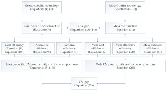
Figure 3.
The flowchart of the methodology section.
3. Results
3.1. Data and Descriptive Statistics
Considering the comparison between regions and regional heterogeneities, the empirical study in this paper can be assessed based on the data of provinces. We viewed 30 provinces as DMUs, and the data sample included the thermal power industry of each province. Due to the fact that we lacked related data, we excluded Tibet, Hongkong, Taiwan, and Macao from the sample. Taking the availability and statistical consistency of the data into account, we selected 2013–2017 as the research period. Furthermore, the choice of variables, to some extent, was determined by the real production process and the data availability [39]. According to the practical production process of thermal power, the inputs of the process are raw material, generating equipment, and labor. Additionally, the power plants need electricity to run, so the auxiliary power should be incorporated into the production process. To sum up, the inputs in this study were labor, energy consumption, installed capacity, and auxiliary power consumption. In view of the fact that there is power dispatching between provinces, electricity can support the local economy. In terms of the approach from Wang et al. [8], “GDP supported by power” is viewed as one of the desirable outputs. The power generation is also included in the desirable outputs. Corresponding to the four input variables, we utilized average wage, standard coal price, generator cost, and electricity price, corresponding to the labor, energy consumption, installed capacity, and auxiliary power consumption, as the input price variables. The detailed information of variables and data sources are displayed in the Table 1.

Table 1.
Variables and data sources.
In order to study the regional heterogeneities among region, we divided 30 tested provinces into the eastern, central, and western regions based on the previous studies [40,41,42,43,44,45].
As shown in Table 2, the average labor in the western region was higher than other two regions, in line with the fact that the total population continues to migrate towards the eastern region. East China had the highest energy consumption among these regions, because the eastern region has developed industry, high population density, and rapid economic development. The eastern region also has the highest average values of installed capacity, power generation, auxiliary power consumption, GDP, average wage, CO2 emissions, generating cost, and electricity price. As the economy of the western region lags behind the other two regions, its value of GDP supported by power was much lower than that of the other two regions. For the standard coal price, the same price is adopted nationwide, so there was no difference in the values of this variable.
Table 2.
Descriptive statistic of variables among three regions.
The energy consumption of the eastern region was 2019.30 mt in 2013, and then gradually grew to 2174.24 mt in 2017, which was similar to the change trend of energy consumption in the western region. The energy consumption of the central region was stable between 1120 mt and 1190 mt during the sample period, indirectly indicating that the central region had effectively slowed down the rising trend of energy consumption. The installed capacity of the three regions all showed an upward trend. In addition to the central region, the other two regions saw significant growth in power generation. In all three regions, there was a rapid increase in GDP supported by power due to the rising in inputs. Only the western region saw a slight increase in total carbon dioxide emissions, while the other two regions held their emissions fairly steady during the sample period. This indirectly reflected the government’s effective control of carbon emissions in recent years.
3.2. Estimated Results of CMPI and Cost Efficiency
Table 3 presents the empirical results of meta-cost-efficiency and its decompositions among these three regions from 2013 to 2017. With respect to the meta-cost-efficiency (CE*), the eastern region outperformed the other two regions, although none of them did particularly well in CE* because their values were lower than 0.7. The average values of CE* in three regions were, respectively, 0.504, 0.313, and 0.290. The major reason for the low CE* was that the meta-allocative-efficiencies (AE*) of these three regions were relatively low compared with the meta-technical-efficiencies (TE*). Additionally, the changing trend of CE* was basically similar with that of AE*. In the eastern region, the TE* performed well during the period 2013–2017, but its value fluctuated up and down between 0.833 and 0.855. However, in central China, the TE* presented a trend of gradual increase, while that of the western region was opposite. The changing trend of AE* in the central region was similar with that of TE*. During the period 2013–2016, in the western region, the value of AE* gradually decreased from 0.380 to 0.343, then rose to 0.366 in 2017. The results of the AE* showed that the most recent allocation of inputs in the eastern region was obviously more suitable than other two regions under the environment of the meta-production-technology. On the basis of meta-technology, compared with the other two regions, the input mix of east China had a better performance regarding CE*, which obviously extended to group-specific production technology.
Table 3.
Meta-cost-efficiency and its break down.
Table 4 presents that the eastern region was more cost-efficient than the other two regions in terms of the meta-production-technology, which was the case in the results of the group-specific production technology. Similarly to the estimated results of CE* and its decompositions among these three regions, the average values of CE showed that group-specific CE of the eastern region was much higher than the that of other two regions. The TE in the eastern region was relatively stable, and the TE in the central region showed a gradual upward trend. In the western region, the value of group-specific TE was greater than that of the meta-TE, indicating that the thermal power production technology has been improved effectively. For the technical efficiency, all three regions performed well. Nevertheless, the western region was closer to its own cost frontier with a greater mean of TE (0.908) than the average of 0.877 and 0.889 in the other two regions, respectively. The same performance as AE* existed in the values of group-specific AE. Based on the group-specific technology, the eastern region still performed best in the allocation management. Similarly to the results of TE*, the eastern, central, and western regions all did well in the group-specific TE during the period 2013–2017.
Table 4.
Group-specific cost efficiency and its decomposition.
Table 5 presents the empirical results of CEG and its divisions under the group-specific technology. We note here that the value of CEG was greater than 1, indicating that the group-specific CE was superior to the CE*. This was the same for the TE and AE. The averages of CE gap for these three regions were, respectively, 1.190, 1.537, and 1.703, which indicate implicit savings of 19.0%, 53.7%, and 70.3%, approximately, if the same outputs were generated under the meta-techniques. Thus, in the western region, the group-specific CE was far superior to the CE*. However, the thermal power production frontier of eastern region was much closer to the meta-frontier with a mean of 1.044 versus 1.055 and 1.149 of the other two regions, respectively. The estimated results of AEG signify that AE based on the group-specific technology was superior to the AE based on the meta-technology among these three regions. As a result of the misallocation of inputs, the cost increase based on the region-specific technology of about 14.2%, 45.7%, and 48.2% were less than those based on the meta-technology in these three regions, respectively. Compared to the other two regions, during the same period, the eastern region was characterized with higher cost efficiency and higher allocative efficiency. To sum up, central and western China can use the experience of the eastern region in the allocative management of inputs for reference.
Table 5.
Group-specific cost efficiency gap and its decomposition.
Table 6 presents the estimated results of group-specific CM productivity and its decompositions. We note here that the change of CM productivity was due to the cost variation in efficiency and the cost variation in the technology. Furthermore, according to Equation (20), group-specific CMt,t+1 can be divided into the growth of CE (CEt,t+1) and CT (CTt,t+1). Then, the CEt,t+1 can be divided into the TE growth (Et,t+1) and AE growth (AEt,t+1). The CTt,t+1 can be broken down into the growth of technology (Tt,t+1) and PE (Et,t+1). The empirical results of CM t,t+1 showed that the three regions all presented a positive cost Malmquist productivity growth from 2013 to 2017, with an annual growth rate of 1.9%, 9.5%, and 4.1% under the group-specific technology, respectively. In the eastern region, the average of ∆CEt,t+1 was 0.972, indicating that there was no big change in cost efficiency. The growth of productivity mainly came from the contribution of the ∆CTt,t+1: 12.3% for the ∆PEt,t+1. For the central region, the increase of CM productivity came from allocative efficiency growth at 4.1% annually and the change of PE at 17.0%. From the perspective of average values, the ∆CEt,t+1 of the three regions all showed a slight decline, mainly due to the annually significant decline in ∆TEt,t+1. On the contrary, the average values of ∆AEt,t+1 and ∆PEt,t+1 displayed increasing trends in all three regions during the sample period.
Table 6.
Group-specific cost Malmquist and its decomposition.
Table 7 presents, firstly, the fact that the group-specific CMPI was higher than the meta-CMPI by 5.9% in central China and by 4.6% in western China annually. The convergence of group-specific CMPI to the meta-CMPI was relatively small. Nevertheless, in the eastern region, the group-specific CMPI regressed over the meta-CMPI by 0.4% annually. When we turn to the components (∆TEG, ∆AEG, ∆TG, ∆PEG) of the CM productivity gap in the eastern region, the group-specific TE, AE, and T of the eastern region catch up with those under the meta-frontier at the annual rate of 2.3%, 1.5%, and 1.7%, respectively. Nevertheless, we can see that the group-specific technology and PE values were less than the meta-frontier ones by 5.7% annually. Additionally, the estimated results of the ∆AEG and ∆PEG in central China were reversed in eastern China from 2013 to 2017. The ∆CEG remained constant and the group-specific AE of the central region was behind in case of the meta-frontier by 2.2% annually. The TE, T, and PE of the central group converged to that of the meta-frontier by 2.2%, 3.3%, and 2.6%, respectively. The changes of the decompositions in the western region were similar to those in the eastern region. The western region’s TE and AE under the group-specific technology also played catch-up with those under the meta-frontier by 2.9% and 3.2% annually.
Table 7.
Cost Malmquist gap and its break down.
The changing trends of Table 7 display that the significant driving factor of the path towards the convergence from group-specific CMPI to meta-CMPI was possibly the TE, input PE, and the changes in T for the central region and also the T on CT for the western region. Moreover, the improvement of TE and AE of input mix drove the convergence in the case of the western region. The estimated results reflect that there is a long convergence path between the group-specific technology and the meta one in the eastern region. To sum up, compared with the other two regions, the eastern regions can be described as having better performance on cost efficiency and allocative efficiency. Moreover, the improvement of TE and AE of the input mix drove the convergence in the case of the western region. The estimated results reflect that there is a long convergence path between the group-specific technology and the meta-technology in the eastern region. To sum up, compared with the other two regions, the eastern regions can be described as having better performance on cost efficiency and allocative efficiency, indicating that the provinces in the central and western regions can learn from the experiences in production cost management and resource allocation management in the eastern region. In order to better understand the cost efficiency and productivity changes of China’s thermal power industry, the estimated results obtained in this paper were compared with the results from the research of Wang et al. [8], mainly because their research methods related to CE were somewhat similar to those of this paper. In their study, they also found that provinces located in the eastern region had higher CE and AE compared to the central and western regions, and 30 provinces all performed well in TE over the period of 2000–2010. Consistent with their findings, we found that CM productivity is increasing in all three regions. The major differences lie in the fact that we found the main driving factor for the increase of CM productivity to be the promotion of allocative efficiency and price effect, while their study found that the main driving factor was the significant improvement of technical efficiency and production technology. In our study, both TE and T had not made significant progress over the study period, which indirectly means that there is still a large space for improvement and optimization in the production technology and production process management of the thermal power industry in China.
3.3. BCG Matrix Analysis
In addition to the analysis about the estimated results of group-specific CMPI and the breakdown of these, we utilized the matrix proposed by the Boston Consulting Group (BCG) to analyze and make the comparison of provincial meta-CMPI data and the breakdown of these results. Based on the empirical results of meta -TE, -AE, -T, and -PE, the pure meta-productivity was calculated by the sum of meta-TE and meta-T, which was viewed as the Y-coordinate. The meta-PE was used as the X-coordinate to compare the growth of price effect among provinces. We took the 1.00 and 1.00 as the midpoints of the meta-productivity and meta-PE, respectively. Four quadrants corresponded to four different types of performance on productivity and price effect. If the meta-productivity and meta-PE were both greater than 1, this indicated that it was a high-performing province in the thermal power industry, which is called the professional province. If the meta-productivity was greater than 1.00 and meta-PE was less than 1.00, this signified that it was a province that benefitted from the price effect, but met productivity has not risen significantly. We describe it as a divisional province. If the meta-productivity was less than 1.00 and meta-PE was less than 1.00, this indicated that there was no positive price effect and significant productivity growth in this province, which is described as a stalemate. In the fourth quadrant, meta-PE was greater than 1.00 and meta-productivity was less than 1.00, this type of province is described as price benefit.
Hence, this paper applied the BCG matrix to assess the performance of meta-productivity and meta-PE in the Chinese thermal power industry of each province as shown in Figure 4. In this figure, A represents professional (higher productivity and higher price effect), B represents divisional (higher productivity and lower price effect), C represents stalemate (lower productivity and lower price effect), and D represents price effect (lower productivity and higher price effect). Only three provinces belonged to the professional type, which implies that these provinces had positive price effect and effectively improved their own production technology and technical efficiency. They can be set as the benchmark for other provinces and just need to maintain the present development status. For instance, as the “experimental field” of electric power reform, Guangdong began to carry out the reform of the electricity sale side in accordance with the requirements of supply-side structural reform in 2013. Guangdong’s electricity market and trading platform were built to allow enterprise and users that meet the standards to enter the market, and then the cost of electricity generation and consumption was reduced through effective market transactions, which may have improved the price effect to a certain extent. Additionally, since 2014, the Energy Bureau of Jiangxi has adopted the optimization evaluation system for the thermal power industry to promote the production technology of thermal power generation, improve production efficiency, and effectively deal with issues about post-production environmental pollution. There were11 provinces described as price beneficial, signifying that they failed to take advantage of the price effect to optimize their technology and technical efficiency. These provinces can improve production technology and adjust production management mechanisms to promote productivity. Nearly half of the provinces were divisional type, implying that they have not adjusted their cost structure and price management effectively, despite improvements in technology and technical efficiency. They can recalculate and plan the input cost and make full use of the price advantage given by the related policy. With the same number as the first quadrant, there were three provinces belonging to the stalemate type. They have to learn from the experience of the benchmark and make the adjustment on input price and production.
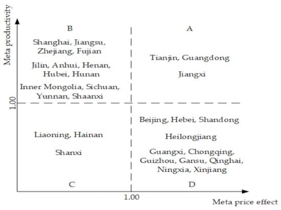
Figure 4.
BCG matrix analysis of meta productivity and meta price effect.
4. Conclusions
Viewing the 30 tested Chinese provinces as DMUs and dividing them into eastern, central, and western regions, we took the changes of input prices and the hidden cost of carbon emissions into consideration. DMUs in different regions had heterogeneity in economic development, production technology, natural resources, and production environment. It is essential to consider the heterogeneity across regions (groups). Therefore, we extended the CMPI in the framework of a meta-frontier to take the heterogeneity across regions (groups) into account and evaluate the CM productivity. The DEA approach was also applied to the meta-CE and group-specific CE of the thermal power industry. We used the cost CM gap to measure the convergence of the group-specific production cost to the production cost under the meta-frontier technology. The BCG matrix analysis was utilized in this paper to make the comparison of meta-productivity and meta-price-effect among provinces. We found the following conclusions and relevant policy implications:
- (1)
- During the sample period, the CE of the eastern region outperformed that of the other two regions every year on the basis of group-specific technology and meta-technology. The main reason why the CE of the eastern region was much higher than the other two regions was that the AE of the eastern region was higher. Compared to the other two regions, the eastern region can be described as more cost efficient, with good technical efficiency and higher allocative efficiency.
- (2)
- The CM productivity in all three regions showed a gradual increasing trend, among which the central region presented the largest progress, followed by the western region. The cost efficiency declined slightly in all three regions. The growth of price effect and allocative efficiency was the main driven factor for the growth of CM productivity in these three regions.
- (3)
- The CM productivity of central and western regions in the case of group-specific technology gradually converged to that in case of meta-technology. The progress of technical efficiency, price effect, and technology were the major factors to promote the growth rate of group-specific CMPI faster than the meta-CMPI. Only in the eastern region did the CM productivity show divergence between the group-specific and meta-frontier, which was mainly derived from the divergence of price effect.
We suggest that thermal power plants in the central and western regions should adjust their mixed fuel structure in order to promote the allocation and management of production resources in the thermal power industry. The local governments should continue to increase investment in research and development of high technologies related to environmental protection and energy saving. As for the thermal power plants in the eastern provinces, there were some effective methods for them to promote technical efficiency, such as improving the operational efficiency of electric generators or replacing inefficient generator sets. All thermal power plants must strictly comply with environmental protection regulations issued by the government to reduce carbon emissions gradually.
Further studies can collect more detailed and useful information to represent the unit prices of inputs in each province. Additionally, machine learning can be used to forecast the changes of inputs and outputs in the next five or ten years and evaluate the CM productivity and cost efficiency, which may come up with more suitable policy implications.
Author Contributions
Conceptualization, X.C. and X.Z; methodology, X.C. and X.Z.; validation, Y.W., X.Z., and Z.Z.; formal analysis, X.Z.; investigation, X.Z.; data curation, X.Z.; writing—original draft preparation, X.Z.; writing—review and editing, X.Z. and X.C.; supervision, X.C. and Z.Z; project administration, X.Z.; funding acquisition, X.C. All authors have read and agreed to the published version of the manuscript.
Funding
This research was funded by Zhejiang Provincial Natural Science Foundation of China under Grant No. LQ21G010006.
Institutional Review Board Statement
Not applicable.
Informed Consent Statement
Not applicable.
Data Availability Statement
Data are not publicly available.
Conflicts of Interest
The authors declare no conflict of interest.
Appendix A
Table A1.
List of abbreviations.
Table A1.
List of abbreviations.
| Abbreviations | Interpretation |
|---|---|
| CM | Cost Malmquist |
| CMPI | Cost Malmquist productivity index |
| DEA | Data envelopment analysis |
| CE | Cost efficiency |
| CT | Cost technology |
| TE | Technical efficiency |
| AE | Allocative efficiency |
| T | Technology |
| PE | Price effect |
Appendix B
Making the assumption that there are K (K = K1 + …+ KJ) DMUs for each t (t = 1, 2, …, T) time period. At t period, in j (j = 1, 2, …, J) group, the kth (k = 1, 2, …, Kj) DMU utilized a vector with N inputs (, , …, ) to generate a vector with M desirable outputs (, , …, ) and H undesirable outputs (, , …, ). Therefore, the corresponding group-specific DF can be calculated by the mathematical programming based on the group’s observations, which is presented as follows:
Similarly to the Equation (A1) above, of the cross period can be measured through the following programming:
where the other group-specific DFs, such as and , can be assessed by changing the time periods in Equations (A1) and (A2).
Now turn to minimum cost function, on the basis of the above assumption, we also assumed that the current input prices (, , …, ) and then the production cost at t time period can be defined as (). Similarly, other production cost functions can also be defined as , . Further, the group-specific minimum cost function at period t can be estimated by the following programming:
The cross period can be calculated by the following:
where the other group-specific cost functions can also be computed by changing the time period in Equations (A3) and (A4).
With respect to the meta-DF based on the meta-technology, such as Equations (2) and (3), , and , and the meta-minimum-cost-functions, such as Equations (4)–(6) and , we applied the same procedure as Equations (A1)–(A4) to collect observations from all groups.
References
- Hoegh-Guldberg, O.; Jacob, D.; Taylor, M.; Bolaños, T.G.; Bindi, M.; Brown, S.; Camilloni, I.A.; Diedhiou, A.; Djalante, R.; Ebi, K.; et al. The human imperative of stabilizing global climate change at 1.5°C. Science 2019, 365, 6459. [Google Scholar] [CrossRef] [PubMed]
- Lelieveld, J.; Klingmüller, K.; Pozzer, A.; Burnett, R.; Haines, A.; Ramanathan, V. Effectsof fossil fuel and total anthropogenic emission removal on public health and climate. Proc. Natl. Acad. Sci. USA 2019, 116, 15. [Google Scholar] [CrossRef]
- Yu, B.; Fang, D.; Dong, F. Study on the evolution of thermal power generation and its nexus with economic growth: Evidence from EU regions. Energy 2020, 205, 118053. [Google Scholar] [CrossRef]
- IPCC. IPCC Special Report on the Impacts of Global Warming 1.5 °C. 2018. Available online: https://www.ipcc.ch/sr15/ (accessed on 10 February 2020).
- Ou, X.M.L.; Yan, X.Y.; Zhang, X.L. Life-cycle energy consumption and greenhouse gas emissions for electricity generation and supply in China. Appl. Energy 2011, 88, 289–297. [Google Scholar] [CrossRef]
- Zhao, X.L.; Lyon, T.P.; Song, C. Lurching towards markets for power: China’s electricity policy 1985–2007. Appl. Energy 2019, 94, 148–155. [Google Scholar] [CrossRef]
- Lam, P.L. Pricing of electricity in China. Energy 2004, 29, 287–300. [Google Scholar] [CrossRef]
- Wang, Y.S.; Xie, B.C.; Shang, L.F.; Li, W.H. Measures to improve the performance of China’s thermal power industry in view of cost efficiency. Appl. Energy 2013, 112, 1078–1086. [Google Scholar] [CrossRef]
- Wang, K.; Zhang, J.M.; Wei, Y.M. Operational and environmental performance in China’s thermal power industry: Taking an effectiveness measure as complement to an efficiency measure. J. Environ. Manag. 2017, 192, 254–270. [Google Scholar] [CrossRef]
- Li, H.Z.; Tian, X.L.; Zou, T. Impact analysis of coal-electricity pricing linkage scheme in China based on stochastic frontier cost function. Appl. Energy 2015, 151, 296–305. [Google Scholar] [CrossRef]
- Chitkara, P. A data envelopment analysis approach to evaluation of operational inefficiencies in power generating units: A case study of Indian powerplants. IEEE Trans. Power Syst. 1999, 14, 419–425. [Google Scholar] [CrossRef]
- Pahwa, A.; Feng, X.; Lubkeman, D. Performance evaluation of electric distribution utilities based on data envelopment analysis. IEEE Trans. Power Syst. 2003, 18, 400–405. [Google Scholar] [CrossRef]
- Wang, K.; Wei, Y.M.; Zhang, X. A comparative analysis of China’s regional energy and emission performance: Which is the better way to deal with undesirable outputs? Energy Policy 2012, 46, 574–584. [Google Scholar] [CrossRef]
- Mou, D. Understanding China’s electricity market reform from the perspective of the coal-fired power disparity. Energy Policy 2014, 74, 224–234. [Google Scholar] [CrossRef]
- Zhou, W.; Zhu, B.; Fuss, S.; Szolgayová, J.; Obersteiner, M.; Fei, W. Uncertainty modeling of CCS investment strategy in China’s power sector. Appl. Energy 2010, 87, 2392–2400. [Google Scholar] [CrossRef]
- Charnes, A.; Cooper, W.W.; Rhodes, E. Measuring the efficiency of decision making units. Eur. J. Oper. Res. 1978, 2, 429–444. [Google Scholar] [CrossRef]
- Färe, R.; Grosskopf, S.; Logan, J. The relative efficiency of Illinois electric utilities. Resour. Energy. 1983, 5, 349–367. [Google Scholar] [CrossRef]
- Olatubi, W.O.; Dismukes, D.E. A data envelopment analysis of the levels and determinants of coal-fired electric power generation performance. Util. Policy 2000, 9, 47–59. [Google Scholar] [CrossRef]
- Shephard, R.W. Theory of Cost and Production Functions; Princeton University Press: Princeton, NJ, USA, 1970. [Google Scholar]
- Färe, R.; Grosskopf, S.; Yaisawarng, S.; Li, S.K.; Wang, Z. Productivity growth in Illinois electric utilities. Resour. Energy 1990, 12, 383–398. [Google Scholar] [CrossRef]
- Yunos, J.M.; Hawdon, D. The efficiency of the national electricity board in Malaysia: An intercountry comparison using DEA. Energy. Econ. 1997, 19, 255–269. [Google Scholar] [CrossRef]
- Abbott, M. The productivity and efficiency of the Australian electricity supply industry. Energy. Econ. 2006, 28, 444–454. [Google Scholar] [CrossRef]
- Chung, Y.H.; Färe, R.; Grosskopf, S. Productivity and undesirable outputs: A directional distance function approach. J. Environ. Manag. 1997, 51, 229–240. [Google Scholar] [CrossRef]
- Kumar, S. Environmentally sensitive productivity growth: A global analysis using Malmquist–Luenberger index. Ecol. Econ. 2006, 56, 280–293. [Google Scholar] [CrossRef]
- Lam, P.L.; Shiu, A.A. data envelopment analysis of the efficiency of China’s thermal power generation. Util. Pol. 2001, 10, 75–83. [Google Scholar] [CrossRef]
- Yu, W.; Jamasb, T.; Pollitt, M. Does weather explain cost and quality performance? An analysis of UK electricity distribution companies. Energy Policy 2009, 37, 4177–4188. [Google Scholar] [CrossRef]
- Kaneko, S.; Fujii, H.; Sawazu, N.; Fujikura, R. Financial allocation strategy for the regional pollution abatement cost of reducing sulfur dioxide emissions in the thermal power sector in China. Energy. Policy 2010, 38, 2131–2141. [Google Scholar] [CrossRef]
- Assaf, A.G.; Barros, C.P.; Managi, S. Cost efficiency of Japanese steam power generation companies: A Bayesian comparison of random and fixed frontier models. Appl. Energy 2011, 88, 1441–1446. [Google Scholar] [CrossRef]
- Zhang, N.; Zhou, P.; Choi, Y. Energy efficiency, CO2 emission performance and technology gaps in fossil fuel electricity generation in Korea: A meta-frontier non-radial directional distance function analysis. Energy Policy 2013, 56, 653–662. [Google Scholar] [CrossRef]
- Chang, T.P.; Hu, J.L. Total-factor energy productivity growth, technical progress, and efficiency change: An empirical study of China. Appl. Energy 2010, 87, 3262–3270. [Google Scholar] [CrossRef]
- Bi, G.B.; Song, W.; Zhou, P.; Liang, L. Does environmental regulation affect energy efficiency in China’s thermal power generation? Empirical evidence from slacks-based DEA model. Energy. Polocy 2014, 66, 537–546. [Google Scholar] [CrossRef]
- Duan, N.; Guo, J.P.; Xie, B.C. Is there a difference between the energy and CO2 emission performance for China’s thermal power industry? a bootstrapped directional distance function approach. Appl. Energy 2015, 162, 1552–1563. [Google Scholar] [CrossRef]
- Yan, D.; Lei, Y.; Li, L.; Song, W. Carbon emission efficiency and spatial clustering analyses in China’s thermal power industry: Evidence from the provincial level. J. Clean. Prod. 2017, 156, 518–527. [Google Scholar] [CrossRef]
- Huang, M.Y.; Juo, J.C.; Fu, T. Metafrontier cost Malmquist productivity index: An application to Taiwanese and Chinese commercial banks. J. Prod. Anal. 2014, 44, 321–335. [Google Scholar] [CrossRef]
- Pastor, J.T.; Lovell, C.A.K. A global Malmquist productivity index. Econ Lett. 2005, 88, 266–271. [Google Scholar] [CrossRef]
- Caves, D.W.; Christensen, L.R.; Diewert, W.E. The economic theory of index numbers and the measurement of input, output and productivity. Econometrica 1982, 50, 1393–1414. [Google Scholar] [CrossRef]
- Färe, R.; Grosskopf, S.; Norris, M.; Zhang, Z. Productivity growth, technical progress, and efficiency change in industrialized countries. Am. Econ. Rev. 1994, 84, 66–83. [Google Scholar]
- Maniadakis, N.; Thanassoulis, E. A cost Malmquist productivity index. Eur. J. Oper. Res. 2004, 154, 396–409. [Google Scholar] [CrossRef]
- Feng, C.; Huang, J.B.; Wang, M. Analysis of green total-factor productivity in China’s regional metal industry: A meta-frontier approach. Resour. Policy 2018, 58, 219–229. [Google Scholar] [CrossRef]
- Lin, B.; Zhang, G. Energy efficiency of Chinese service sector and its regional differences. J. Clean. Prod. 2017, 168, 614–625. [Google Scholar] [CrossRef]
- Eguchi, S.; Takayabu, H.; Lin, C. Sources of inefficient power generation by coal-fired thermal power plants in China: A metafrontier DEA decomposition approach. Renew. Sustain. Energy. Rev. 2021, 138, 110562. [Google Scholar] [CrossRef]
- Feng, C.; Wang, M.; Zhang, Y.; Liu, G.C. Decomposition of energy efficiency and energy-saving potential in China: A three-hierarchy meta-frontier approach. J. Clean. Prod. 2018, 176, 1054–1064. [Google Scholar] [CrossRef]
- Zhou, Y.; Xing, X.; Fang, K.; Liang, D.; Xu, C. Environmental efficiency analysis of power industry in China based on an entropy SBM model. Energy. Polocy 2013, 57, 68–75. [Google Scholar] [CrossRef]
- Chen, X.; Zhang, X.; Wu, X.; Lu, C.C. The environmental health and energy efficiency in China: A network slacks-based measure. Energy Environ. 2021. [Google Scholar] [CrossRef]
- Chen, X. Exploring the sources of financial performance in Chinese banks: A comparative analysis of different types of banks. N. Am. Econ. Financ. 2020, 51, 101076. [Google Scholar] [CrossRef]
Publisher’s Note: MDPI stays neutral with regard to jurisdictional claims in published maps and institutional affiliations. |
© 2021 by the authors. Licensee MDPI, Basel, Switzerland. This article is an open access article distributed under the terms and conditions of the Creative Commons Attribution (CC BY) license (https://creativecommons.org/licenses/by/4.0/).