Social Uncertainty Evaluation of Social Impact Bonds: A Model and Practical Application

Francesco Rania; Annarita Trotta; Rosella Carè; Maria Cristina Migliazza; Abdellah Kabli

doi:10.3390/su12093854

,

and

¹

Department of Law, Economics and Sociology, University Magna Graecia of Catanzaro, Campus Germaneto, Viale Europa, 88100 Catanzaro, Italy

²

Department of Economics and Business, University of Cagliari, Viale S. Ignazio 17, 09125 Cagliari, Italy

^*

Author to whom correspondence should be addressed.

Sustainability2020, 12(9), 3854;https://doi.org/10.3390/su12093854

This article belongs to the Special Issue Finance and Agenda 2030: Building Momentum for Systemic Change—A Special Issue Coordinated by the Sustainable Finance Group of SDSN France

Version Notes

Order Reprints

Abstract

In the last years, Social Impact Bonds (SIBs) have gained popularity in the impact investing space. A number of scholars and practitioners are debating—in theory and practice—the opportunities, challenges and obstacles of these financial models. Amongst others, social uncertainty evaluation metrics appear as a critical factor for the future development of the SIB market. The present work aims to shed some light on this issue, by realizing a practical application of a model—which is an extension of a framework previously proposed—for social uncertainty evaluation in SIBs. In our exploratory analysis, 34 SIBs were selected for the empirical tests. We combined the Analytic Hierarchical Process (AHP) with the creation of aggregate measure, deriving by suitable indicators at the end of the tree. Our findings open new avenues for future research in the field of uncertainty factors in the SIB landscape. Finally, our results represent a basis for implementing a prediction model for social uncertainty evaluation.

Keywords:

social impact bonds; impact investing; social uncertainty; decision-making under uncertainty; analytic hierarchy process

1. Social Impact Bonds and Social Uncertainty: Setting the Context

The purpose of this exploratory study is to realize a practical application of a model for social uncertainty evaluation in Social Impact Bonds (SIBs).

Since their introduction in the United Kingdom in 2010, SIBs have become popular in the academic, practitioner, and policy-maker world [1,2]. 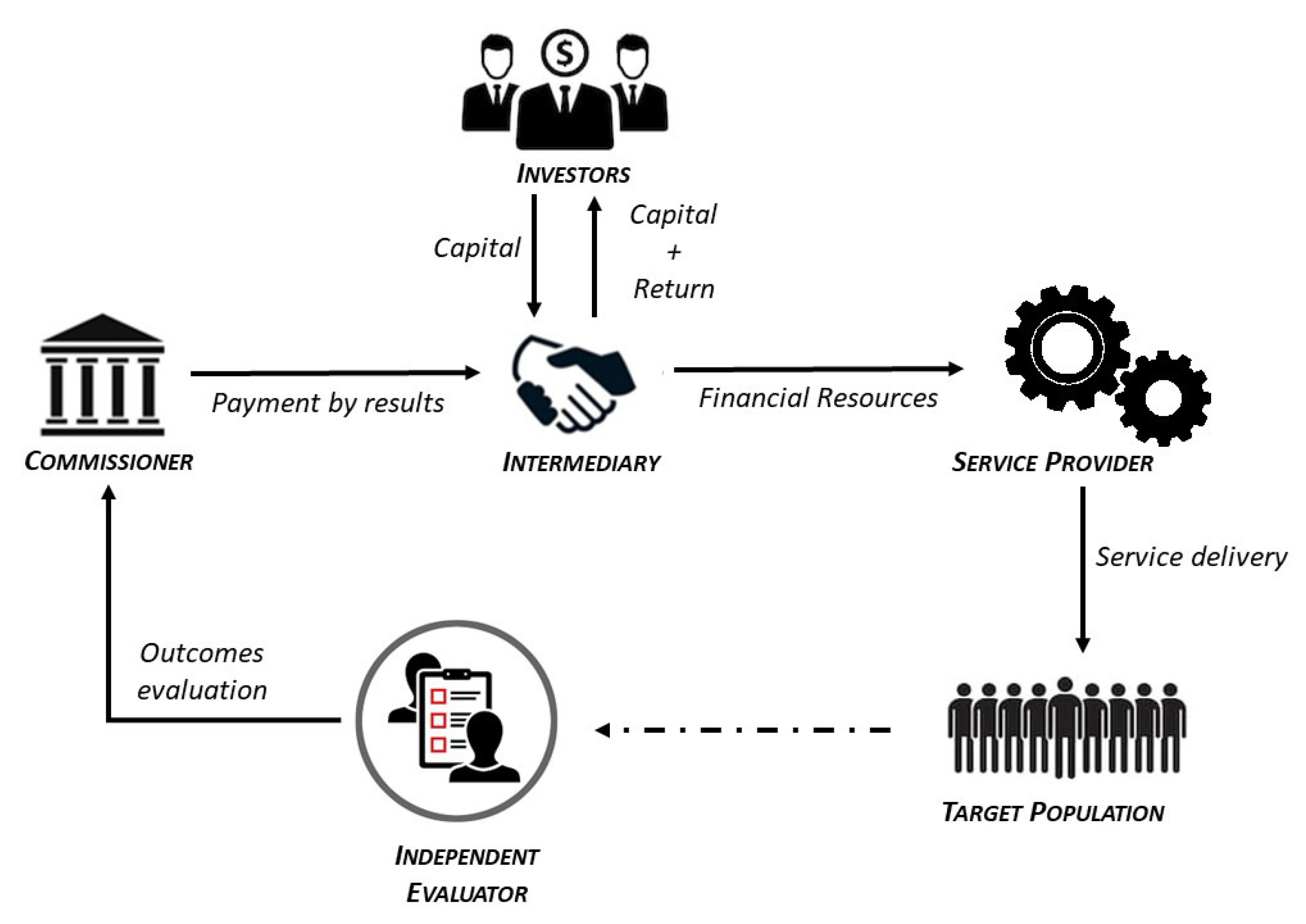In the impact investing arena, SIBs are an interesting innovative financial mechanism [3], that seem to promise a solution for financing complex social interventions [4] and reallocate performance and financial risk from the public towards the private sector ([5], p. 41). More in detail, SIBs have been defined as “payment by results contracts that leverage private social investment to cover the up-front expenditure associated with welfare services” ([6], p. 57). According to ([7], p. 1), payment-by-results (PbR) is a scheme for “delivering public services where the government (or the commissioner) pays providers for the outcome they achieve rather than the activities they deliver”.

A literature overview provided by ([8], p. 72) discusses the main characteristics of PbR: (1) contingent payments depend on independent verification of results; (2) the PbR contracts should include both reward and penalties useful for achieving the outcomes; (3) risk transfer exists and depends on both the impact and the success of the project. SIBs are a form of PbR, but SIBs extend PbR by harnessing social investment from capital markets to cover (partly or fully) the costs of service intervention [6].

Therefore, investor return depends on the impact of the project and on the achieving outcomes [9]. The key point in the SIBs (and PbR) schemes is the outcome measurement, and, accordingly, the quality of the performance measure (see Section 2.1).

On the theoretical level, several scholars note that the opportunities related to the SIB market development are vast and perhaps endless [5], but, at the same time, challenges and obstacles are often highlighted [10]. The complexity of the SIBs schemes is evident (see Section 2.1): they are characterized by public–private partnerships [1] between several counterparties, and each actor has different interests, goals, and expectations, and different risk attitudes and perceptions [11].

On the empirical level, examining the evidence from the SIB market, it is worth noticing that the diffusion of SIBs is still modest. From the launch, in 2010, of the first pilot SIB in the UK (HMP Peterborough) to the end of October 2019, only just over 130 SIBs have been implemented worldwide [12]. Among these, only 34 are closed. It is clear that the limited size of the SIB market clashes with the theoretically great potential of SIBs.

The risk (or uncertainty) issue represents one of the main controversial points related to the use of SIBs on a larger scale [5,13,14] and, at the same time, it is still underexplored [15,16,17]. It is clear that the complexity of the SIBs model increases the probability of SIBs failing. On the other hand, some scholars are underlying downsides and risk facets of SIB models (see Section 2.1).

More generally, with regards to the impact investing field—of which SIBs are key components—some scholars are exploring, amongst other things, social risk [18,19,20,21,22], impact risk [23,24,25,26], social uncertainty [27,28], and their linkages and differences [27], by also using methods and approaches very different from those of traditional mainstream finance. Impact investing is considered a “revolutionary” way to improve sustainability. Impact investing is characterized by the explicit intention (intentionality), social purpose, and the ability to generate positive environmental and/or social impact in accordance with an appropriate risk-return investment [11]. It is important to note that “intentionality” represents the linkage between ethics and facts, thus determining a consequentiality between (positive) values and value creation. These innovative approaches open new views for research on how finance should be “reconsidered” [29,30,31], and also question the foundations of the mainstream finance [32].

In order to shed light on these open problems, some works are focusing on SIBs’ practices to better understand risks (or uncertainty) related to SIBs’ contractual schemes and social and financial features [1,5,16]. In the light of the social impact investing approaches, a constant focus on social risk (rather than on other risks) certainly favors a more effective social finance capital allocation and reminds us that the first purpose of social finance is to bring about maximum social change rather than to make money ([33], p. 308).

To the best of our knowledge, only very few works, such as Scognamiglio et al. [5,22], have proposed a framework able to support the evaluation of an SIB, starting from a measurement of the social uncertainty (for a discussion of these previous works see Section 3.1, in which we also explain several main alternative approaches to the impact evaluation). These works open new promising avenues for researches, useful to promote the development of SIB models, on large scale.

However, currently, regarding the SIBs, there are still no definite and effective models (already widely tested and used) capable of evaluating the social uncertainty. Starting from these works, we attempt to test an implemented model—which is an extension of a framework proposed by [5]—capable of providing final scores related to social uncertainty evaluation of the overall population of SIBs closed worldwide at the end of October 2019. As far as we are aware, this is the first analysis using all of the closed extant SIBs. Our work offers some preliminary but significant results on social uncertainty, which is one of the most relevant and underexplored issues of SIBs. In addition, it proposes a quantitative measure of several qualitative key elements related to the SIB Programs, providing useful suggestions for investors and other stakeholders. Then, it realizes an in-depth comparison of several SIB programs and an insight of market practices. Finally, this pilot study is a retrospective analysis and represents a first step towards implementing a prediction model for social uncertainty evaluation.

In our work, we use the following definition of social uncertainty provided by ([5], p. 42): “most definitions interpret social uncertainty as the risk of not reaching the intended impact [18] or as the likelihood that a given allocation of capital will generate the expected social outcomes irrespective of any financial returns or losses [27]. Despite this heterogeneity of definitions, social uncertainty could be considered more generally as a concept providing an indication of the certainty that an output will lead to the stated impact [26].”

The choice to focus on uncertainty (rather than risk) deserves some clarification.

Knight [34] established a clear difference between the concepts of “risk”and “uncertainty”. The famous phrase “uncertainty is an unknown risk, whilst risk is a measurable uncertainty” underlines the fact that risk refers to situations that can be quantitatively measured through a distinct probability distribution; on the other hand, uncertainty refers to those events for which there is not enough knowledge to identify objective probabilities. Therefore, the revolutionary works of Knight shed light on different facets of concepts of uncertainty and show the limitedness of the mechanical analogy in understanding enterprise and profit ([35], p. 458). In this vein, Knight’s view is a challenge to neoclassical theory [35]: uncertainty arises out of partial knowledge ([35], p. 459) and this concept represents the turning point for advancing in psychological decision theory, such as a host of psychological insights beyond the risk–uncertainty distinction ([36], p. 458). In more detail, Knight described features of risky choices that were to become the key components of prospect theory (Kahneman and Tversky [37]): the reference-dependent valuation of outcomes and the non-linear weighting of probabilities.

Based on these considerations, Knight’s view is a useful starting point for our exploratory analysis: risk is objective since it represents a variable independently of the individual; uncertainty is, on the contrary, subjective, because it depends on the individual, their information, and their temperament. Hence, a decision under the conditions of uncertainty has a higher impact than one made under the conditions of risk, both for the decision maker and for the context in which they operate. The tools used to analyze risk and uncertainty are different, too. For risk statistical techniques are used, whilst for uncertainty heuristic ones are used [38].

From this point of view, our application appears particularly interesting, because its focus is on social uncertainty (rather than on social risk), following Knight’s view: it overcomes the limitations of the traditional finance paradigm (and of its mechanistic models) by leading towards more complete foundations for building momentum for systemic change. In addition, our analysis uses a modified Analytic Hierarchic Process (AHP) that consists of combining any leaf with the hierarchy tree; typical of such a multi-criteria method, indicators with appropriate measuring scales are capable of describing the characteristics of the problem. Compared to the previous methods [5,39,40], our implemented technique offers the advantage of obtaining more flexible adjustments and implementations in terms of levels of investigation, indicators, and scales. These characteristics seem to be particularly useful for better understanding SIB model dynamics and peculiarities (see Section 2.1 and Section 3.1).

2. Background

2.1. The SIB Model: Key Elements

Built around a collaborative public–private contract, SIBs represent a new funding model that aims to improve service quality and to enhance the social outcomes achieved by using private resources rather than public funding. Proponents of SIBs often suggest that these new schemes have the capacity to leverage additional resources for innovative services that will help, in the near future, to improve social outcomes and cost savings for the public commissioner [6]. The introduction of private principles and actors through outcome-based commissioning has received a great deal of attention in recent years [6]. The SIB model was first proposed in Peterborough (United Kingdom) in 2010 and has quickly spread internationally and across different sectors [13].

SIBs involve payment-by-results (PbR) through a contract between public service providers and private investors [41], in which investors provide the upfront financing to service providers for the interventions that target a social outcome. At the same time, the commissioner (also named the outcome payer) makes PbR payments based on the level of social outcomes achieved. The interplay between all the involved actors is represented in Figure 1.

Figure 1. The SIB model.

The implementation of SIB projects begins when the commissioner (usually a public entity, at the national or local level) identifies a certain social need and target population and enters a contract with the intermediary [42]. After receiving the working capital needed from the intermediary, the service provider delivers a pre-agreed-upon set of outcomes [17]. The outcome measurement represents a key element for SIBs: the independent evaluator assesses their final level and only in the case of achievement of the pre-defined social outcomes does the commissioner provide payments.

In summary, the SIB structure transfers the risk of poor performance from the commissioner to the investors; investors receive a financial return for taking this risk, as well as a social return through the outcomes achieved (a ‘blended return’).

The combination of the different actors involved in an SIB project is part of the innovation [43], and it enables the public sector to commission innovative services by sharing the risk of exploring a new welfare approach and investors to provide working capital for social projects by receiving both a financial and a social return [42].

SIBs are not suited to every project, but rather depend on specific criteria [42,44], such as the presence of a clear and measurable outcome.

Despite the growing interest shown by both academics and practitioners, the numbers of SIBs activated worldwide is exhibiting a slowdown (see [12] ).

From a theoretical point of view, recent works seems to focus on SIBs’ downsides by criticizing the marketization of the delivery of traditionally public services, the effective ability to lead to better outcomes, and the value they provide compared with their cost structure and the additional transaction and administrative costs they generate [10,16,45,46,47,48].

The debate appears polarized around a series of recurrent aspects [49], including those that describe SIBs as a model framed to transfer risks usually retained by the public sector to the private sector. Under this perspective, only a limited number of works tried to understand the risks related to similar initiatives [5,42,50,51,52].

2.2. The SIB Market: Characteristics and Trends

According to the Social Finance Database [12], 137 Impact Bonds (IBs) have been launched around the world (with a total amount of raised capital of about $440 M). More in detail, 130 of these are SIBs, whereas 7 can be defined as Development Impact Bonds. Table 1 shows the number of SIBs implemented by country.

Table 1. Numbers of SIBs implemented by country worldwide.

The SIBs launched covered several social issue areas (e.g., workforce development, housing/ homelessness housing, health, child and family welfare, criminal justice, education and early years, and poverty and environment).

According to the Governemnt Outcomes Lab [53] (GO Lab), 34 SIBs have been completed in nine different countries. Among these, the “HMP Peterborough (The One Service)” and the “NYC Adolescent Behavioral Learning Experience Project for Incarcerated Youth (NYC ABLE)” were closed before completion. Table A1 (see Appendix A.1) provides an overview in terms of the “socio-demographic” data of the closed SIBs, with a focus on the investors involved in each SIB project. Table 2 shows the capital raised and the number of SIBs launched/completed for social issue worldwide.

Table 2. Capital raised and SIBs launched, implemented, and completed for each social issue area worldwide.

3. Method, Model Description and Data Collection

3.1. Methodological Approach

In this work we attempt to measure the uncertainty of SIBs by combining a multi-criteria decision method with a process for constructing composite indicators. We test a model that is an extension and an improvement of [5]. In [5], social uncertainty evaluation in SIBs was hierarchically explained involving 3 main categories, 5 factors and 16 sub-factors. Scognamiglio et al. [5], in turn, referred to Serrano-Cinca and Gutierrez-Nieto [40], where the goodness of investment in Social Venture Capital (SVC) was evaluated through a model hierarchically structured in 3 principal factors, 26 criteria, and 160 indicators, as suggested by a small group of SVC’s analysts and academics. Furthermore, the same structure of model in [5] was used in Scognamiglio et al. [22] to explore the relationship between social risk and financial return within the context of SIBs.

Starting from these previous works, our model uses the multi-criteria decision method, the aggregation techniques, and the measuring scales in a different manner.

Among the different multi-criteria decision methods, AHP is suitable for its versatility in different fields (see Saaty [39]) and for solving complex problems after disassembling the phenomenon into criteria (e.g., categories, factors, and sub-factors) and assigning a priority to each of them.

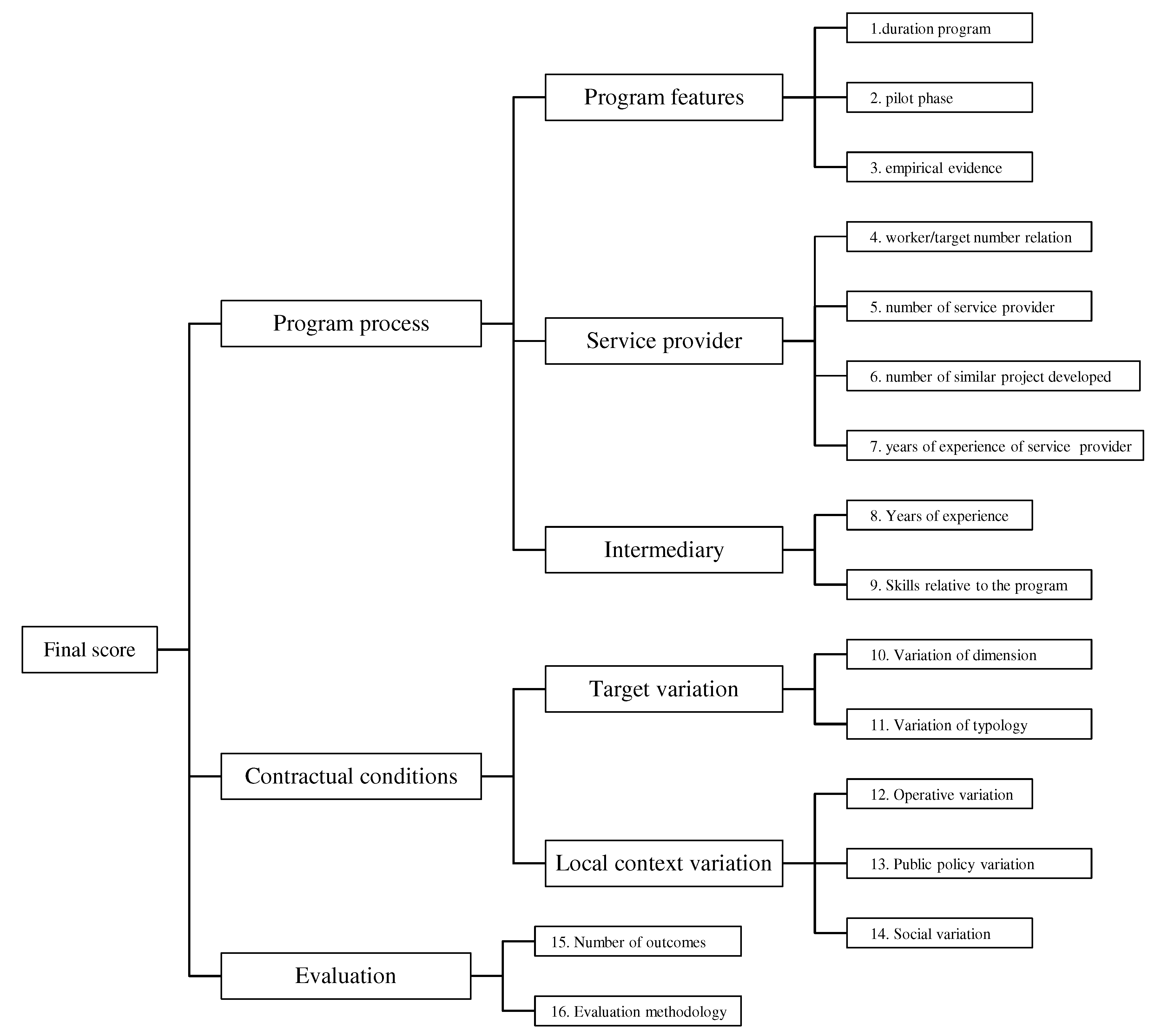
In order to the design the model, an SIBs uncertainty score is given using an aggregation process where the elements, similarly to [5] in type, number, and position, are placed over a three-level tree diagram. At the first level there are three main categories; at the second level, five factors are divided into two groups, and two indicators are linked to an upper category; and at the third level, 14 indicators are grouped around the upper factors. Figure 2 shows the diagram tree used in detail.

Figure 2. The hierarchal structure of the SIBs problem.

In our study, despite [40], AHP is applied only for the first two levels of the diagram tree (categories and factors) and, differently from [5], the same is separately repeated for groups of the same level. The computation of weights for the different levels allows us to obtain a final scoring of immediate interpretation without using the comparisons typical of AHP. Furthermore, the computation of weight for different groups reduces the error in terms of consistent judgments (see Appendix B.1).

The explorative nature of our analysis and the absence of a large dataset required the use of alternative statistical techniques (with respect to the classical ones such as factorial analysis, cluster analysis, etc.). In addition, it is worth emphasizing that these techniques need strong assumptions not available in our context (see, e.g., normality conditions).

Our analysis also realized pilot interviews for scholars with extensive experience in the SIBs field (via questionnaire) in order to compare all pairwise elements belonging to the same hierarchical level and concerning the common upper aspect.

Table 3 presents the experts’ pairwise comparisons among the criteria and the weights of each criteria, in accordance with Figure 2.

Table 3. Experts’ priorities.

In particular, the comparisons were made by the experts for groups of the same level, using the 9-point Saaty scale (in which 1 = “two criteria are equally important”and 9 = “the first criterion is absolutely more important than the second”, 3, 5, 7 denote respectively slight, medium, and strong importance, while

\frac{1}{3}

,

\frac{1}{5}

,

\frac{1}{7}

, and

\frac{1}{9}

assume the reciprocal sense). The results are the entries of the so-called Pair Comparison Matrices (PCMs) (see the matrices in columns 3, 5, and 7 of Table 3). Each PCM then produces the priorities of the criteria involved (see the percentages in columns 4, 6, and 8 of Table 3). Thus, for example, if we consider how the expert #R1 evaluates the categories, then her PCM can be read: “Program Process”and “Contractual Condition” contribute equally to uncertainty (value = 1); while both “Program Process”and “Contractual Condition” are strongly more uncertain than “Evaluation” (value = 5); and by contrast, “Evaluation” is strongly more certain (value =

1 / 5

) both than “Program Process”and “Contractual Condition”. By this PCM, the priorities of “Program Process”, “Contractual Condition” and “Evaluation” are 45.5%, 45.5%, and 9.1%, respectively.

The composite indicators have been constructed by using the min-max normalization procedure with an objective weighting method and a weighted mean as the aggregation function.

In particular, the min-max normalization method (see [54], Table 3, p. 30) is a linear transformation that scales the data between 0 and 1 after subtracting the minimum value and successively scaling the data to the range of the collected data. This type of normalization allows us to free all indicators from their unit of measurement and to mark those unnecessary, which will hence be deleted from the next computation.

The weighting procedure restitutes an objective value proportional to the length of the measuring scale used and near to the ideal one. In fact, despite [5], a wider 5-point Likert scale (1 = randomized control Trial, 2 = quasi-experimental, 3 = validate administrative data, 4 = historical comparison, and 5 = unavailable) is used to measure the indicator “Evaluation methodology”. In this case, the additional and better specified attributes (one more than [5] and with a well-balanced scale as suggested by Go LAB) allow us partially to offset the structural gap among categories. In particular, with regard to the distribution of indicators (12.5% in “Evaluation”, 31.3% in “Contractual conditions” and 56.3% in “Program process”), “Evaluation methodology” has 66.7% priority in its category and 6.67% more than its corresponding priority in [5]. This positive variation multiplied by the difference of the scores in “Evaluation“ contributes to improving our model. Moreover, involving the indicators with the longest scales (“Evaluation methodology” and “Number of Outcomes”), this variation is fundamental for the “Evaluation” category and, more in general, provides a better basis for carrying out the uncertainty.

In conclusion, the SIBs uncertainty is a number ranging from 0 to 1 (with 0 = absolute certainty and 1 = absolute uncertainty).

3.2. The Model

We start from the diagram tree shown in Figure 2 to explain the model. We use the following graphic symbols to specify the position of each element involved and its relationships with others:

-: ℓ := level;
-: $m^{(ℓ)}$ := elements (categories, factors, indicators) in the level ℓ;
-: $Λ^{ℓ}$ := compositions of the elements in the level ℓ;
-: k:= label of the group of elements shared by a characteristic;
-: $G_{k}^{(ℓ)}$ := group of elements shared by a characteristic in the level ℓ.

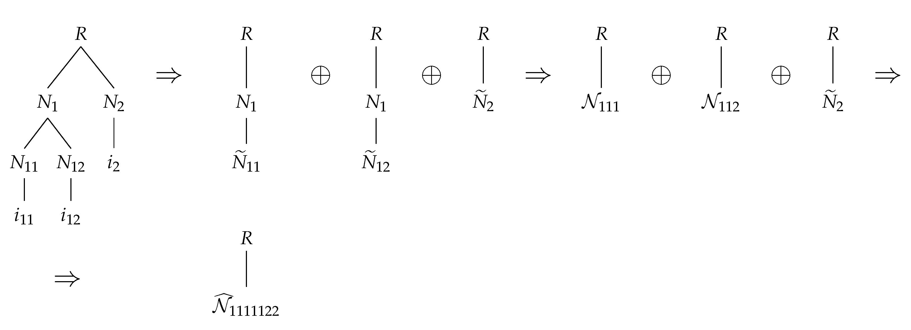
The final score is intended as the result of the following phases:

Phase 1 or Preparation of data.: For every SIBs i, transform the information relative to any indicator n placed at the level ℓ inside the group $G_{k}^{(ℓ)}$ , in a number $x_{i n k}^{(ℓ)}$ taking into account the measuring scale adopted in terms of uncertainty (e.g., on a 3-point Likert scale 1 is the best value and 3 the worst value). Normalize all indicators’ scores in pure numbers $x_{i n k}^{(ℓ)}$ over a ratio scale to homogenize the different ranges.
Phase 2 or Priorities of categories and factors.: Compare all the elements that refer to the same aspect pairwise (categories with categories, factors with factors). Build thus the Pairwise Comparison Matrices $A_{k}^{(ℓ)}$ and, after proving the sufficient consistency for each of them, estimate the weights $w_{i n k}^{(ℓ)}$ using the principal eigenvector method. The ranking thus obtained will be used only when the procedure arrives at the level where these elements are.
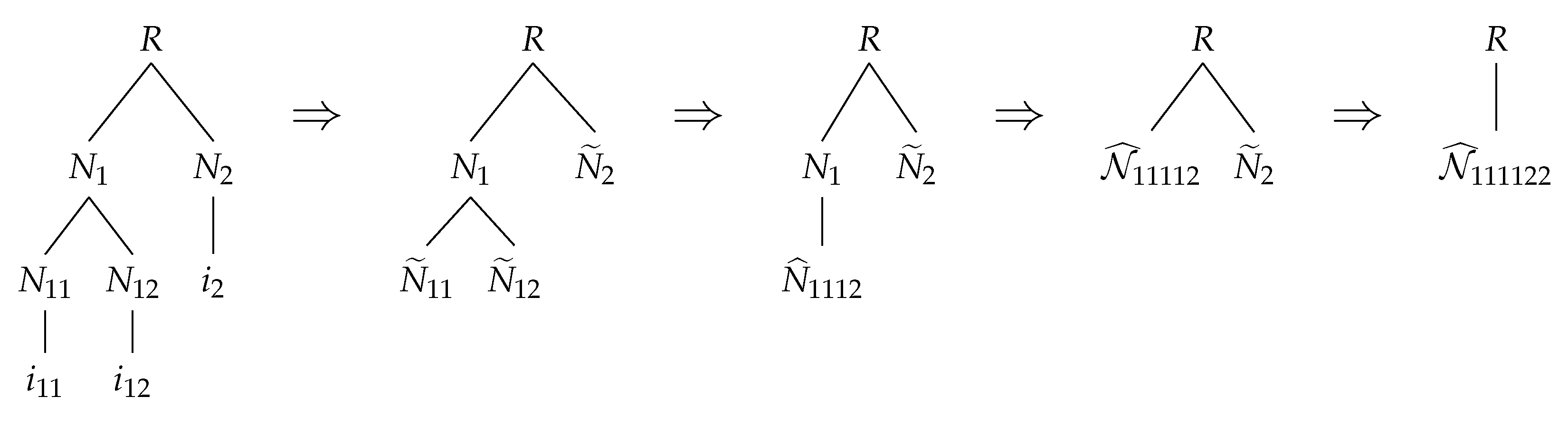
Phase 3 or Total aggregation.: Aggregate the scores of the indicators which refer to the same aspect to obtain the composite indicators:

$M^{W} (X_{i n}^{(ℓ)}) : = \sum_{k} x_{i n k}^{(ℓ)} w_{i n k}^{(ℓ)}$

Continue the aggregative process, going up to the next level, while taking into account the weights previously computed by the related PCM. When the first level (goal) is achieved, the process is ended and the final score thus obtained for aggregation gives us the measure of uncertainty:

$F S : = \sum_{ℓ} \sum_{k} M^{W} (X_{k}^{(ℓ)}) W_{k}^{(ℓ)}$

For more clarification on the mathematical tools and model, see Appendix B and Appendix C.

3.3. Sample and Data Collection

For this pilot analysis, a practical application was tested by using a “population” of SIBs (see Appendix A). The sample was not randomly selected. In more detail, SIBs must be closed (as of the end of October 2019), and they have to comply with the requirements of the transparency and verifiability of information.

To evaluate the model (specified in the previous sections) and its usefulness, we tested it by using data collected from 34 SIBs. More in detail, we tested the model using two types of data: the objective publicly available data (through the Government Outcomes Lab—GO Lab—database and other sources) relatively to scales and units of indicators, and the subjective data through a preliminary survey (via questionnaire) to obtain the priorities among factors and categories of our factor tree.

Two junior researchers separately selected publicly available material on online databases and publicly available material from other sources. Subsequently, senior researchers checked the information drawn up and created a protocol to use relevant information for analysis, ensuring research quality and rigor.

With regard to the survey, we selected the experts using the following criteria:

Criterion 1:: the experts on SIBs are selected within those who authored or co-authored peer-reviewed chapters of books and books on the topic area;
Criterion 2:: the experts have published at least one research article evaluating and/or measuring aspects of SIBs in prestigious international journals.

In August and September 2019, we found through Google Scholar (using search terms in line with Criteria 1 and 2) a total of 26 potential works in line with Criterion 1 and only 10 in line with Criterion 2. The experts were selected if they met at minimum one of the criteria. Finally, 3 experts were selected (of which 11.5 % are in line with the first criterion and 33.3% with all criteria). From a statistical point of view, the size of this sample guarantees a standard error of

\pm 7.2 %

with a 99.5% confidence level on the reliability of the prioritizing method.

Furthermore, the experts were also consulted to refine the structure of the diagram tree.

3.4. The Sample: A Focus on Key Characteristics

We have analyzed for each of the 34 completed SIBs the following key characteristics:

Duration: length of providing services (expressed in years);
Financial resources:
-
Max outcome payments: total outcome payments (expressed in home country currency);
-
Capital raised: capital invested by the investors (expressed in home country currency);
Service provider: a private for-profit or not-for-profit organization to deliver social services;
Number of outcomes: number of outcomes defined by the project;
Target population: people to which an outcome is targeted;
Intermediaries: subjects involved to coordinate investor(s), service provider(s) and evaluator(s).

We assigned a number (from 1 to 34) for each of the 34 SIBs analyzed in our work in order to simplify the elaboration and presentation of our study (see Appendix A).

These 34 completed SIBs at the end of October 2019, according to the GO Lab Database, represent about 25% of the total number of SIBs launched worldwide.

With regard to our “population”, we have analyzed in depth:

All types of SIBs structures (direct, managed, and intermediated, in accordance with the Goodall approach [55]);
All categories of outcomes evaluation methodology (randomized control trial, quasi-experimental, validate administrative data, and historical comparison in accordance with Gustafsson-Wright et al. [56]);
The main service providers involved in two or more SIBs, in accordance with Social Finance UK (Buzinezzclub, Thames Reach, Core Assets, Career Connect, Teens and Toddlers, Action for Children);
The most important intermediaries specialized and involved in SIBs, such as Social Finance UK and Triodos Bank UK, in accordance with Calderini et al. [57];
All financial aspects;
All outcomes achieved.

For detailed information about these key characteristics of the SIBs analyzed in our model see Table A2 in Appendix A.

Despite this, our “population” shows some limitations regarding “capital raised” and “issue area”.

Analyzing the “capital raised”, our “sample” has reached about $50 million compared to $440 million. These 34 completed SIBs show, on average, a low amount of “capital raised”.

In accordance with Social Finance UK, the major investments have been made in United States since 2013, seeing that 26 projects were launched that correspond to $219 million of “capital raised”. The projects that were launched covered vast territories and/or a high number of people. These big projects are still being implemented and should be finished within the next few years. Only one of these big projects (NYC Adolescent Behavioral Learning Experience Project for Incarcerated Youth) has been concluded and was included in our “population”.

Comparing the characteristics of the “issue area” between our sample and all of the SIBs launched around the world, we noted that our “population” lacked two new important issue areas, in accordance with the categories defined by Social Finance: “health” and “poverty and environment”.

SIBs for the health sector are called Health Impact Bonds (HIBs) and they represent a new method of financing the health sector, as observed by Rizzello et al. [8], which has always been characterized by financial deficit. These HIBs have developed in many parts of the world since 2015, not only in developing countries but also in industrialized countries. Currently, there are 22 HIBs launched in many countries all over the world. These projects are still being implemented according to the GO Lab database, and will be concluded within a few years.

There were three SIBs addressed to a “Poverty and environment” issue launched between 2016–2019. These projects were launched in the USA, The Netherlands, and in Uganda and will be concluded in the next few years. Currently, these types of SIBs are in the implementation phase, according to the GO Lab database.

In our sample, most of the SIBs analyzed were concerned with “Workforce Development” and “Homelessness” social issues (see Table 2).

For an overview in terms of the “socio-demographic” data of the sample with a focus on the investors involved in each SIB project, see Table A1 in Appendix A.1.

4. Application, Model Validation and Analysis

4.1. Practical Application

The model in Section 3.2 was tested on completed 34 SIBs.

Throughout this work, we use the following notation:

- A = Program duration;	- P = Social variation;
- B = Pilot phase;	- Q = How many outcomes are measured;
- C = Empirical evidence;	- R = Which methodology is used;
- D = Worker/target number relation;	- $A + B + C$ = Program features;
- E = Number of service providers;	- $D + E + F + G$ = Service provider;
- F = Number of similar projects developed;	- $H + I$ = Intermediary;
- G = Years of experience of service provider;	- $L + M$ = Target variation;
- H = Years of experience;	- $N + O + P$ = Local context variation;
- I = Skills relative to the program;	- $A + B + C + D + E + F + G + H + I$ = Program process;
- L = Variation of dimension;	- $L + M + N + O + P$ = Contractual conditions;
- M = Variation of typology;	- $Q + R$ = Evaluation;
- N = Operative variation;	- $A + B + C + D + E + F + G + H + I + L + M + N + O + P + Q + R$ = Final score.
- O = Public policy variation;

In Table 4 the numerical values of

m^{(ℓ)}

,

Λ^{(ℓ)}

, k, and

G^{(ℓ)}

are presented according to Figure 2.

Table 4. Panel of SIBs uncertainty’s diagram tree.

The uncertainty score of each SIB has been calculated from the data collected (see Table 5, variables A, B, …, R) following the phases described in Section 3.2.

Table 5. SIBs data collection from GO Lab.

The data were normalized with the formula (A6) for obtaining basic homogenous indicators labeled by the italic letters running from A to R (see Appendix D, Table A5). In our study, the variable “P” is constant and assumes a minimum value (=1), so its normalization P loses sense (see Appendix D, Table A5, label N/A) and allows us to mark it as a variable not useful to the computation. As said in Section 3.1, this fact is explained thus: “Social Variation” is a consolidated practice for all SIBs and is also less significant than others to measuring the SIB uncertainty.

We then horizontally aggregate the normalized data (see Appendix C, Figure A2 and formula (A12)) for groups and thus obtain the composite indicators. Thus, for example, if the variables A, B, and C are selected and afferent to the same group (see column 4 and row 4 of Table 4), their aggregation determines the indicator, or more precisely, the factor

A + B + C

= “Program Features”. For example, in the case of SIB number 29, the values will be:

A + B + C = 0.50 \times 0.50 + 0.00 \times 0.25 + 1.00 \times 0.25 = 0.500

.

In our diagram tree, the majority of indicators is placed at the third level (see row 4 of Table 4 in correspondence to n). Therefore, the resulting composite indicators are the factors placed at the second level (see Appendix D, Table A6).

After deleting P, the resulting composite indicator “Local Context Variation”, given by the aggregation of only N and O, is lighter. In the case of the variables Q and R, they are on the second level (see also

n = 2

in Table 4), and hence the resulting composite indicator is the category “Evaluation”.

The “subjective” aggregation has been made by using the weights given by the experts (see Section 3.1, Table 3 and Appendix D, Table A7). Finally, Table 6 shows the result for each considered SIB and for each expert by obtaining the final score.

Table 6. Uncertainty score per expert.

Hence, for example, if we consider SIB 29 and the weights of expert #R2, the uncertainty score is:

F S = (0.750 \times 0.333 + 0.571 \times 0.333 + 0.00 \times 0.333) \times 0.455 + (1.000 \times 0.50 + 0.000 \times 0.50) \times 0.455 + 0.167 \times 0.091 = 0.40108

.

4.2. Model Validation

We validated the model starting from the three final scores provided by our experts (see Table 6). The question is whether these differences are such as to affect the model and the construction of the final score (see formula A19). In this respect, we conducted a descriptive analysis and a robustness analysis.

4.2.1. Descriptive Statistics

The final score data of #R1 and #R2 have a moderate range (0.3343 and 0.2616, respectively) excluding the outliers (SIB 1, 29, 32 for #R1 and SIB 7, 14, 23 for #R2); they are close to a mean (0.4269 and 0.3900, respectively) since they have a low standard deviation (0.0765 and 0.0685, respectively). By contrast, the data of #R3 are very variegated (0.1045 of std. dev.), but tend on average to a lower value of uncertainty (mean of 0.3268); they are also equally distributed into the interquartile range (IQR) and along the whiskers, and none of them are outliers.

Finally, we observe that the IQRs of #R1 and #R2 contain SIBs with moderate uncertainty, while the IQR of #R3, ending at a lower value than others (percentile 75 = 0.3631), contains SIBs that are quite certain.

The main statistics are presented in Table 7.

Table 7. Statistics of final scores by experts.

We use the Spearman correlation (

ρ

) and the absolute mean difference (

| Δ r |

) to measure the pairwise diversity among three dataset.

While #R1 and #R2 do not differ greatly in judgments (

ρ = 0.766

and

| \bar{Δ r} | = 4.824

), just like #R2 and #R3 (

ρ = 0.637

and

| \bar{Δ r} | = 5.353

), #R1 and #R2 are, instead, rather far away in community (

ρ = 0.306

and

| \bar{Δ r} | = 7.765

).

4.2.2. Robustness Check

We examined the robustness of the model through the extent to which results are affected by the indicators used. In the present case, we compared the final score with the one obtained, every time omitting one indicator in turn.

In Table 8, we present the results of such a sensitivity analysis conducted for any expert by using the Spearman coefficient. The final scoring is substantially stable with the exception of one indicator for #R2 (L) and #R3 (F), and of two indicators for #R1 (L and M).

Table 8. Sensitivity results omitting one indicator in turn.

For every expert, the largest contribution to the final scoring is principally given by the indicators into “Local Context variation” and “Evaluation” (correlation close to 1.000). In minor measure, the uncertainty depends on the indicators into “Program Features” and in “Intermediary” (correlations around 0.990 and 0.930, respectively). Finally, the rest of the indicators participate moderately in the score, according to the experts considered.

4.3. Main Findings

4.3.1. Results from Model Application: Some Non-Relevant Indicators

Our analysis highlights the presence of indicators without relevance. As previously mentioned in Section 4.1, indicator “P” has the same value for all of the 34 SIBs and refers to the question “is the program developed in the same social and local context?”. This indicator is probably not relevant to our analysis because usually SIBs are developed for a specific project, to be implemented in a specific area in which the social need has been previously detected and with a limited possibility of social variation. Thus, to avoid differences among the different cohorts in which the program will be implemented, these should have the same “social or local”characteristics.

An indicator that is strictly connected to our indicator “P”, even though it is enclosed in the factor “Local Context Variation”, is indicator “M”(Variation of typology). As summarized in Table 5, indicator “M”shows the same value (=2) for all of the SIBs enclosed in our sample except for SIBs 12, 13, 14, and 27 (=1). Indicator “M”refers to the question “does the contract permit the ongoing variation of target typology?”. Like indicator “P”, indicator “M”is constant (except in four cases). Overall, this means that 88% of our cases do not show any kind of ongoing variation of target typology during the implementation stage and, like in the case of indicator “P”, the motivation relies to the fact that these two aspects are often tightly defined in the contract.

In order to better understand this aspect, we linked our result to the case of Peterborough SIB. We know that this SIB has been implemented by the UK Ministry of Justice to provide ’through-the-gate’ and post-release support to prisoners serving short sentences to reduce reoffending in a group of 3000 adult males (aged 18 or over) who received custodial sentences of less than 12 months [44,49]. As clarified by FitzGerald et al. [49], the cohort was very tightly defined and composed only of individuals with prison sentences of less than 12 months and in which everyone eligible has been contacted by the delivery organization[s] even though participation was voluntary. Eligibility criteria for prisoners to enter the cohort were defined in the contract.

Overall, this implies that the possibility of target variation should have been included in the contract. This aspect is the same for 88% of our sample. The case of Peterbough is also useful to explain results for indicator “O”(Public policy variation). Looking inside Table 5, indicator “O”shows a different value only for Peterbough SIB (value = 1) that could be considered as a unique case, considering that it was the first to be implemented and the only one in which a policy reform caused the cancellation of the third cohort [42,58].

Other indicators that show a limited information power are the pilot phase (B), empirical evidence (C), and years of experience of the service provider (G). Regarding indicator “B”, only in the “London Homelessness Social Impact Bond (Thames Reach)”SIB the value is different (value = 2) in respect to the others (value = 1), while regarding indicator “C”only in the SIBs “DWP Innovation Fund Round II—Thames Valley (Energise)”, “DWP Innovation Fund Round II—West London (Prevista)”, and “the Benevolent Society Social Benefit Bond”the value is different (value = 1) in respect to the others (value = 2).

Indicator “B”corresponds to the question “is a pilot phase present?”and it is differentiated from the others only by the fact that this information is not disclosed or not available for this SIB. Finally, both indicators “B”and “C”are enclosed in the factor “Program features”. This implies that the factor “Program feautures” is almost entirely explained by the indicator “A” (program duration).

Regarding indicator “G”that corresponds to the question “how many years of experience do the older service providers involved in the program have?”, it assumes a different value (value = 2) in respect to the others (value = 1) only in the SIBs “London Homelessness Social Impact Bond (St Mungo’s/Street Impact)”and “Fair Chance Fund—West Yorkshire (Fusion Housing)”.

4.3.2. Differences between Experts’ Preferences and Weights and Uncertainty Scores

Responses provided by our three respondents (#R1, #R2, #R3) highlight differences both in the categories and factors suggested (see Table 3).

As synthesized in Table 3, regarding our categories, #R1 and #R2 showed the same level of agreement around the three categories, while #R3 showed a high preference for the first category (“Program process”) and a lower preference (11.1%) for the second and third. This means that for #R3 the first category was more important than the other two. Regarding our factors, the preferences of #R2 were equally distributed between “Program Feautures”, “Service Provider”, and “Intermediary”(0.50), and between “Target variation”and “Local context variation”. By contrast, #R3 provided a different perspective by reducing the importance of the factor “Program features”and of “Local context variation”.

Differences in respondents’ weights and preferences correspond to a high variance among the overall scores for each of the SIBs. Table 9 summarizes SIBs with the highest level of uncertainty by the respondents.

Table 9. SIBs with the highest level of uncertainty by respondent.

As emphasized in Table 9, #R1 and #R2 show a high level of uncertainty for the following SIBs: “Buzinezzclub Programme (Rotterdam)”, “Academia de Còdigo Jùnior Lisbon”and “Perspective: Work”. #R2 and #R3 show a high level of uncertainty for the following SIBs: “Youth Engagement Fund—Unlocking Potential/Career Connect (Greater Merseyside)”and “DWP Innovation Fund Round I—East London (Links for Life)”. No SIBs are in common between #R1 and #R3.

It is interesting to note that #R1 provided the second highest level of uncertainty associated with the HMP Peterborough SIB that, as highlighted previously, represents the first SIB implemented and the only one discontinued due to a policy reform. This appears to be in line with the preferences, in terms of weights, provided by #R1.

Comparing the lowest scores provided by our respondents and summarized in Table 10, we found that #R1, #R2, and #R3 converge towards the “DWP Innovation Fund Round II—West London (Prevista)”SIB that is also the SIB with the lowest score of uncertainty (and also the absolute lower score). At the same time, #R1 and #R2 show a similar score for the following SIBs: “NYC Adolescent Behavioral Learning Experience Project for Incarcerated Youth” and “DWP Innovation Fund Round II—West London (Prevista)” while #R2 and #R3 show a similar score for the following SIBs: “Fair Chance Fund—Birmingham (Rewriting Futures/St Basil’s)”, “Fair Chance Fund—Liverpool (Local Solutions)”, and “Youth Engagement Fund—Prevista (London)”.

Table 10. SIBs with the lowest level of uncertainty.

By comparing Table 9 and Table 10, it emerges that if #R1 and #R2 consider the SIB “Buzinezzclub Program (Rotterdam)”as the most uncertain, #R3 considers this SIB as less uncertain (27%), and on the contrary while #R1 consider the SIB “London Homelessness Social Impact Bond (Thames Reach)”as one of the less uncertain, the same SIB is considered by #R3 as the most uncertain. The different weights and importances justify these differences (Table 3).

Table 10 highlights a further aspect. In the lists of SIBs with the lower level of uncertainty, #R1 and #R2 signaled the project “NYC Adolescent Behavioral Learning Experience Project for Incarcerated Youth”. However, the“NYC Adolescent Behavioral Learning Experience Project for Incarcerated Youth” SIB was terminated after three years of service delivery when the recidivism rates of the first cohort showed no significant results compared with historical rates [59]. This led us to immediately understand that probably both weights and preferences suggested by #R1 and #R2 focussed on aspects (in the factors tree) that do not capture the possibility that SIBs may fail.

This aspect is particularly impressive. By going back to the respondents’ preferences (see Section 4.3.2 and Table 3) we found that while #R1 and #R2 gave the same attention to the three categories (“Program Process”, “Contractual Conditions”, and “Evaluation”), #R3 showed a high preference for the first category. This probably means that #R3 did not consider this SIB as less uncertain due to the attention given to the “Program Process” category and thus did not consider the possibility that design deficiencies could affect the success of the entire project.

5. Discussion of Results

The results obtained in the analysis highlight the weakness of the factors tree initially developed by Scognamiglio et al. [5]. The analysis revealed the presence of a high number of variables that are not able to capture uncertainty in an SIB project.

Nevertheless, the comparison between our uncertainty scores and the main characteristics of failed SIBs let us detect the need for further variables. Among closed SIBs, the “NYC Adolescent Behavioral Learning Experience Project for Incarcerated Youth” has been considered by two respondents as an SIB with a lower level of uncertainty. The project was launched by Goldman Sachs Bank’s Urban Investment Group (UIG) that announced a $9.6 million loan to support the delivery of the program to a predefined target population. The program was terminated after three years due to the lack of results. Similarly, the SIB “HMP Peterborough (The One Service)” was discontinued due to the “Transforming Rehabilitation” reforms to probation in the United Kingdom.

The “NYC Adolescent Behavioral Learning Experience Project for Incarcerated Youth” was the first SIB launched in the US and was guaranteed by Bloomberg Philanthropies, substantially reducing the downside risk. Conversely, the SIB “HMP Peterborough (The One Service)” was the first SIB launched worldwide and the first attempt to improve a funding mechanism for reducing recidivism among prisoners.

The ex-post analysis of these two SIBs led us to understand that further variables are required in order to capture uncertainty. In particular, further variables should consider the presence of guarantee schemes, the type of social issue addressed, and the voluntary or involuntary engagement of the target population by focusing not only on the contractual conditions of the SIB project but also on the “financial” and “social issue” characteristics.

Moreover, our analysis starts from the definition provided by Nicholls and Tomkinson [27], in which social uncertainty captures endogenous (e.g., organizational/responsiveness) and exogenous (e.g., political, economic, social, technological, and environmental) factors and in which both are negatively correlated to social return. In the case of SIBs, the higher the risk of change in the context in which the social program is delivered, the lower the social return that can be achieved. If the context of a social program changes—as in the case of Peterborough—it is more suitable to disconnect the entire program without further efforts by renouncing the possibility to achieve a lower level of social return (with the related reputational effects). Similarly, future projects in which there is a likelihood of contextual change will fail due to the fewer incentives related to their implementation. In the same way, in the context of endogenous factors, the likelihood that contracts or staff achieve less than optimal results will lead to changes or the termination of the contract before detrimental outcomes (including reputational ones).

In conclusion, the fact that no complete information about the remaining 32 closed SIBs is available does not help us to understand if our score is effectively able to capture their level of uncertainty or if their risk management processes have been able to capture the manifestation of their potential uncertainty factors early. Nevertheless, our analysis reveals that in order to capture the overall uncertainty related to an SIB, further risk factors should be considered by distinguishing among those strictly related to the contractual characteristics of the project (e.g., financial and social issues) and those related to endogenous/exogenous factors that have been not explored before.

These preliminary findings open new avenues for future research in the field of uncertainty and risk factors in the social impact bond landscape.

6. Concluding Remarks, Implications, and Future Research Directions

Our analysis focussed on social uncertainty, meant as the possibility that an SIB could not reach the intended impact or generate the expected social outcomes. The study was conducted in order to apply the model previously developed by Scognamiglio et al. [5] in a practical context by trying to improve it and to understand if and how it was able to reveal uncertainty in SIB projects. By using an “ex-post”approach and the population of closed SIBs, we performed a retrospective test of social uncertainty by considering a given set of variables, factors, and indicators. The results reveal a high number of non-relevant indicators. Further analyses are required in order to transform this retrospective approach into a predictive—and thus standardized—approach useful to evaluate ex-ante the uncertainty level of each new SIB project proposed.

Moreover, while several scholars had pointed out the main characteristics of SIBs, their enabling factors and the main opportunities that come from their implementations, it had remained unclear how to evaluate their level of uncertainty. We have attempted to address this knowledge gap through this work. At the same time, this work contributes to the field of alternative methodological approaches for sustainable finance. Under this perspective, we used an alternative methodological approach that cannot be brought back to the methods of mainstream finance in order to estimate the ability of SIBs to achieve outcomes. This implies not only a methodological shift related to the use of the AHP method—typically used in the social sciences—but also in the conceptual foundation of finance research typically oriented towards a more quantitative aspect and less interested in social purposes.

From a more practical point of view, this work could potentially contribute to the development of the entire SIB market by allowing both practitioners and policy makers to understand the areas from which uncertainty arises and thus helping the development of more focused risk management practices and more standardized SIBs schemes.

Although the findings are encouraging, there are a few limitations that need to be considered when interpreting the results of this study. The first limitation is related to the number of experts interviewed. More respondents would have allowed us to get more information and to achieve more comparisons by allowing us to refine the initial factor tree further. However, considering the exploratory nature of this study and especially our initial aims—testing the uncertainty model in a retrospective manner—this could not be considered as a point of weakness: some non-relevant indicators have been detected as needing further refinements. Future development of the model should consider this aspect as a starting point by considering the opportunity to improve the sample of respondents, and mixing qualitative and quantitative comparisons would help to clarify the validity of the model, also supporting the development of a more fine-tuned weighting scale to reduce subjective biases. The second limitation refers to the fact that we did not consider any interactions between indicators. The simultaneous presence of several elements could potentially reduce or increase the overall level of uncertainty. Finally, our analysis does not consider the presence of a “residual risk” that the model could not be able to capture and the possibility that uncertainty could not be explained without considering aspects such as opportunistic behavior and information asymmetries among the involved parties.

Author Contributions

A.T.: conceived, designed, and supervised the research; F.R.: implemented the model, conducted the formal analysis, and gave valuable advice; R.C.: discussed the results, implications, future research direction and gave valuable advice; M.C.M. and A.K.: searched for data regarding the investigated SIBs. In addition to this, more in detail, A.T. contributed to the Sections: Section 1 and Section 3.3; F.R. contributed to the Sections: Section 3.1, Section 3.2, Section 4.1, Section 4.2, Section 4.2.1, Section 4.2.2, Appendix B, Appendix C and Appendix D; R.C. contributed to the Sections: Section 2.1, Section 4.3, Section 4.3.1, Section 4.3.2, Section 5 and Section 6; M.C.M. contributed to the Section: Section 3.4 and Appendix A.2; A.K. contributed to the Sections: Section 2.2 and Appendix A.1. All authors have read and agreed to the published version of the manuscript.

Funding

This work was realized in the framework of the Project Social Impact Finance (SIF16_00055) “An Italian platform for impact finance: financial models for social inclusion and sustainable welfare”(in collaboration with: Sapienza, University of Rome, Project Leader), funded by the Italian Ministry of the Education, University and Research (MIUR), PNR (2015-2020), DD. 2153, 12.10.2016; DD. 1303, 30.05.2017.

Acknowledgments

The authors would like to express sincere gratitude for the valuable comments and suggestions received by the interviewed colleagues. The Authors would also like to thank the participants of the 3rd Social Impact Investments International Conference (5–6 December 2019, Rome) for their inspiring contributions. Finally, the authors are incredibly grateful to the three anonymous reviewers that have made the effort to review this work and have each contributed to its improvement during the peer-review phase.

Conflicts of Interest

The authors declare no conflict of interest.

Appendix A. The Sample

In this section the sample is described both in terms of socio-demographic and financial characteristics.

Appendix A.1. The Sample: An Overview

Table A1 provides an overview in terms of “socio-demographic”data of the sample, with a focus on the investors involved in each SIB project. In addition, the first column shows the number we assigned to each SIB (and through which we identify each unit of our sample). The last column describes the structure of the SIBs, according to the Goodall [55] approach, which identifies three distinct types: (1) direct, (2) intermediated, and (3) managed.

Table A1. SIB’s Overview.

N.	Country	Name (GO Lab)	Issue Area (Social Finance)	Year of Launch	Investors	Structure
1	UK	HMP Peterborough (The One Service)	Criminal justice	2010	Barrow Cadbury Trust; Esmée Fairbairn Foundation; Friends Provident Foundation; The Henry Smith Charity; Johansson Family Foundation; Lankelly Chase Foundation; The Monument Trust, Panaphur Charitable Trust; Paul Hamlyn Foundation; Tudor Trust; Rockefeller Foundation; Sainsbury’s Charitable Trust and J Paul Getty Charitable Trust	Managed
2	UK	DWP Innovation Fund Round I—West Midlands (The Advance Programme)	Workforce Development	2012	Advance Personnel Management (APM) UK Ltd	Intermediated
3	UK	DWP Innovation Fund Round I—Nottingham (Nottingham Futures)	Workforce Development	2012	Nottingham City Council	Direct
4	UK	DWP Innovation Fund Round I—Greater Merseyside (New Horizons/Career Connect)	Workforce Development	2012	Bridges Ventures; Big Society Capital; Esmee Fairbairn Foundation; Charities Aid Foundation; Knowsely Housing Trust; Helena Partnerships; Liverpool Mutual Homes and Wirral Partnership Homes	Intermediated
5	UK	DWP Innovation Fund Round I—East London (Think Forward/Tomorrow’s People)	Workforce Development	2012	Big Society Capital and Impetus-PEF	Intermediated
6	UK	DWP Innovation Fund Round I—Scotland—Perthshire & Kinross (Living Balance)	Workforce Development	2012	10 local businesses and individuals; a local church and a local funding body	Managed
7	UK	DWP Innovation Fund Round I—East London (Links for Life)	Workforce Development	2012	Bridges Ventures, Stratford Development Partnerships	Intermediated
8	UK	DWP Innovation Fund Round II—Thames Valley (Energise)	Workforce Development	2012	Big Society Capital; Barrow Cadbury Trust; Esmee Fairbairn Foundation; Bracknell Forest Housing Association; Buckinghamshire County Council and Berkshire Community Foundation	Intermediated
9	UK	DWP Innovation Fund Round II—Greater Manchester (Teens and Toddlers)	Workforce Development	2012	Bridges Ventures; Impetus-PEF; Esmee Fairbairn Foundation; CAF Venturesome and The Barrow-Cadbury Trust	Intermediated
10	UK	DWP Innovation Fund Round II—West London (Prevista)	Workforce Development	2012	Prevista	Not publicly available
11	UK	DWP Innovation Fund Round II—Wales—Cardiff & Newport (3SC Capitalise)	Workforce Development	2012	3SC and Big Society Capital	Intermediated
12	UK	Essex County Council Multi-Systemic Therapy (MST)	Child and Family Welfare	2012	Big Society Capital; Bridges Ventures; The Social Venture Fund; Charities Aid Foundation; The King Badouin Foundation; Tudor Trust; Barrow Cadbury Trust and EsmŽe Fairbairn Foundation	Intermediated
13	UK	London Homelessness Social Impact Bond (St Mungo’s/Street Impact)	Housing/ Homelessness	2012	St. Mungo’s Broadway; CAF Venturesome; Department of Health Social Enterprise; Investment Fund; Orp Foundation; Big Issue Invest and Other individual investors	Direct
14	UK	London Homelessness Social Impact Bond (Thames Reach)	Housing/ Homelessness	2012	Thames Reach; CAF Venturesome; Department of Health Social Enterprise Investment Bond; Orp Foundation; Big Issue Invest and Other individual investors	Direct
15	UK	Commissioning Better Outcomes Fund- The Step Down Programme (Birmingham)	Child and Family Welfare	2014	Bridges Ventures	Direct
16	UK	Fair Chance Fund—Manchester, Rochdale, Oldham & Royal Borough of Greenwich (Depaul UK)	Housing/ Homelessness	2015	Big Issue Invest; Bridges Ventures and Montpelier Foundation	Managed
17	UK	Fair Chance Fund—Birmingham (Rewriting Futures/St Basil’s)	Housing/ Homelessness	2015	Big Issue Invest; Bridges Ventures; CAF Venturesome; Barrow Cadbury Trust and The Key Fund	Intermediated
18	UK	Fair Chance Fund—West Yorkshire (Fusion Housing)	Housing/ Homelessness	2015	Bridges Ventures and Key Fund	Intermediated
19	UK	Fair Chance Fund—Liverpool (Local Solutions)	Housing/ Homelessness	2015	Big Issue Invest; Big Society Capital and The Key Fund	Direct
20	UK	Fair Chance Fund—Leicestershire (Ambition East Midlands)	Housing/ Homelessness	2015	Big Issue Invest; The Key Fund and Retail Investors	Direct
21	UK	Fair Chance Fund—Gloucestershire (Aspire Gloucester)	Housing/ Homelessness	2015	CAF Venturesome and Retail Investors	Direct
22	UK	Fair Chance Fund—Newcastle (Home Group)	Housing/ Homelessness	2015	Northstar Ventures	Direct
23	UK	Youth Engagement Fund—Unlocking Potential/Career Connect (Greater Merseyside)	Workforce Development	2015	Bridges Ventures	Not publicly available
24	UK	Youth Engagement Fund- Prevista (London)	Workforce Development	2015	Undisclosed private investors	Not publicly available
25	UK	Youth Engagement Fund—Futureshapers Sheffield (Sheffield)	Workforce Development	2015	The Key Fund	Managed
26	UK	Youth Engagement Fund- Teens and Toddlers (Greater Manchester)	Workforce Development	2015	Bridges Ventures; Esmee Fairbairn and Impetus-PEF	Not publicly available
27	USA	NYC Adolescent Behavioral Learning Experience Project for Incarcerated Youth	Criminal justice	2012	Goldman Sachs Bloomberg Philanthropies	Managed
28	Australia	Benevolent Society Social Benefit Bond	Child and Family Welfare	2013	Australian Ethical Investment and Westpac Foundation	Direct
29	Netherlands	Buzinezzclub Programme (Rotterdam)	Workforce Development	2013	ABN AMRO Social Impact Fund and Start Foundation	Intermediated
30	Germany	Youth with Perspective	Workforce Development	2013	BHF-BANK Foundation; BonVenture; BMW Foundation; Herbert Quandt and Eberhard von Kuenheim Foundation (BMW AG)	Managed
31	Belgium	Duo for a Job (Brussels)	Workforce Development	2014	Unspecified private investors	Direct
32	Austria	Perspective: Work	Child and Family Welfare	2015	ERSTE Foundation; HIL Foundation; Scheuch Family Private Foundation; Schweighofer Private Foundation and Juvatgemeinn ützige GmbH	Not publicly available
33	Portugal	Academia de CòdigoJùniorLisbon	Education and EarlyYears	2015	Calouste Gulbenkian Foundation	Intermediated
34	Colombia	EmpleandoFuturo [Employing the Future]—Colombia Workforce Development SIB	Workforce Development	2017	Fundacion Bolivar Davivienda, Fundacion Mario Santodomingo, Fundacion Corona	Not publicly available

Source: our elaboration from Social Finance Database [12], GO Lab database.

Appendix A.2. The Sample: A Focus on Key Characteristics

Table A2 gives detailed publicly available information on the 34 completed SIBs analyzed in our work.

Table A2. A focus on key characteristics of SIBs.

N.	SIB Name (GOLab)	Duration (Years)	Financial Resources		Service Provider	N. Outcome	Target Population	Intermediary
N.	SIB Name (GOLab)	Duration (Years)	Max Outcome Payments (M)	Capital Raised (M)	Service Provider	N. Outcome	Target Population	Intermediary
1	HMP Peterborough (The One Service)	7	£8	£5	The One Service	2	Adult male prisoners (aged 18 or over)	Social Finance UK
2	DWP Innovation Fund Round I—West Midlands (The Advance Programme)	3.5	£3.4	£3	BEST Network	9	NEET (14–24 years)	APM UK Ltd.
3	DWP Innovation Fund Round I—Nottingham (Nottingham Futures)	3.5	£2.9	£1.7	Nottinghamshire Futures	9	Disadvantaged NEETs (14–24 years)	Nottingham City Council
4	DWP Innovation Fund Round I—Greater Merseyside (New Horizons/Career Connect)	3.5	N/A	£1.5	Career Connect	9	Disadvantaged NEETs (14–24 years)	Triodos Bank UK
5	DWP Innovation Fund Round I—East London (Think Forward/Tomorrow’s People)	3.5	£3.2	£0.9	Tomorrow’s People	9	NEETs	Impetus-PEF
6	DWP Innovation Fund Round I—Scotland—Perthshire & Kinross (Living Balance)	3.5	£1.2	N/A	Perth YMCA	9	NEETs (14–24 years)	Indigo Project Solutions
7	DWP Innovation Fund Round I—East London (Links for Life)	3.5	£1.3	£0.37	Community Links	9	Disadvantaged NEETs (14–19 years)	no intermediary
8	DWP Innovation Fund Round II—Thames Valley (Energise)	3.5	£3.7	£0.9	Adviza	9	Disadvantaged NEETs (14–16 years)	Social Finance UK
9	DWP Innovation Fund Round II—Greater Manchester (Teens and Toddlers)	3	£3.3	£0.8	Teens and Toddlers	9	Disadvantaged NEETs (14–15 years)	Social Finance UK
10	DWP Innovation Fund Round II—West London (Prevista)	3.5	£3	N/A	Prevista	13	Disadvantaged NEETs (14–15 years)	Prevista
11	DWP Innovation Fund Round II—Wales—Cardiff & Newport (3SC Capitalise)	3.5	£1.9	£0.40	Dyslexia Action and Include	10	Disadvantaged NEETs (14–15 years)	3SC
12	Essex County Council Multi-Systemic Therapy (MST)	8	£7	£3.13	Action for Children	1	High-risk adolescents (11–17 years)	Social Finance UK
13	London Homelessness Social Impact Bond (St Mungo’s/Street Impact)	3	£2.4	£1.2	St. Mungo’s Broadway	12	Homelessness	no intermediary
14	London Homelessness Social Impact Bond (Thames Reach)	3	£2.4	£1.2	Thames Reach	12	Homelessness	no intermediary
15	Commissioning Better Outcomes Fund- The Step Down Programme	4	N/A	£1	Core Assets	1	Young people (11–15 years)	no intermediary
16	Fair Chance Fund—Manchester. Rochdale. Oldham & Royal Borough of Greenwich (Depaul UK)	3.5	£1.6	£0.62	Depaul UK	21	Homelessness NEETs (18–24 years)	Social Finance UK
17	Fair Chance Fund—Birmingham (Rewriting Futures/St Basil’s)	3.5	£2.5	£1.03	St. Basil’s	21	Homelessness NEETs (18–24 years)	Social Finance UK
18	Fair Chance Fund—West Yorkshire (Fusion Housing)	3	N/A	£0.84	Fusion Housing	21	NEETs (18–24 years)	Numbers4Good
19	Fair Chance Fund—Liverpool (Local Solutions)	3	£1.2	£0.55	Local Solutions	21	Homelessness NEETs (18–24 years)	Social Finance UK
20	Fair Chance Fund—Leicestershire (Ambition East Midlands)	3	£3	£0.6	YMCA Derbyshire and P3	21	Homelessness NEETs (18–24 years)	Triodos Bank UK
21	Fair Chance Fund—Gloucestershire (Aspire Gloucester)	3	£1.5	£0.31	P3 and CCP	21	NEETs (18–24 years)	Triodos Bank UK
22	Fair Chance Fund—Newcastle (Home Group)	3	N/A	£0.49	Home Group	21	NEETs (18–24 years)	Numbers4Good
23	Youth Engagement Fund—Unlocking Potential/Career Connect (Greater Merseyside)	3	N/A	£1.12	Career Connect	11	Disadvantaged Young people (14–17 years)	no intermediary
24	Youth Engagement Fund- Prevista (London)	3	N/A	N/A	Prevista Ltd	11	Disadvantaged Young people (14–17 years)	Triodos Bank UK
25	Youth Engagement Fund—Futureshapers Sheffield (Sheffield)	3	N/A	£1125	Futureshapers Sheffield	11	Disadvantaged Young people (14–17 years)	Triodos Bank UK
26	Youth Engagement Fund- Teens and Toddlers (Greater Manchester)	3	£3	£0.5	Teens and Toddlers	11	Disadvantaged Young people (14–17 years)	Social Finance UK
27	NYC Adolescent Behavioral Learning Experience Project for Incarcerated Youth	3	$11.7	$7.2	The Osborne Association and Friends of Island Academy	6	High-risk adolescent prisoners (16–18 years)	MDRC
28	Benevolent Society Social Benefit Bond	7	AUD 19.5	AUD 10	The Benevolent Society	3	Families with adopted child (less than 6 years old)	Social Ventures Australia and UnitingCare Burnside
29	Buzinezzclub Programme (Rotterdam)	5	€0.85	€0.72	Buzinezzclub	1	Young people (17–27 years)	Deloitte and Social Impact Finance
30	Youth with Perspective	2	€0.3	N/A	Ausbildungsman—agementAugsburg—Joblingeg GmbH, Jugend und Familienhilfe Hochzoll, Apeirose.V	1	Young people (less than 25 years old)	Juvatgemeinnützige GmbH
31	Duo for a Job (Brussels)	3	€0.29	€0.23	Duo for a Job	1	Young migrants (18–30 years)	Kois Invest
32	Perspective: Work	3	€0.8	N/A	Gewaltschutzzentrum Upper Austria—Frauenhaus Linz	2	Women affected by violence	Juvatgemeinnützige GmbH
33	Academia de CòdigoJùniorLisbon	1	N/A	€0.125	Lisbon primary schools—Junior Code Academy	3	Students	Kois Invest
34	EmpleandoFuturo [Employing the Future]—Colombia Workforce Development SIB	5	N/A	COP 834	Kuepa, Fundacion Colombia Incluyente, FundacionCarvajal, Volver a la gente	6	Unemployed people (18–40 years)	Fundaciòn Corona

Source: our elaboration from publicly available information.

Appendix B. Mathematical Miscellanies

This section presents some mathematical definitions, theorems and procedures useful for the present study.

Appendix B.1. AHP Method

An

n \times n

real matrix

A = (a_{i j})

is said to be positive if

a_{i j} > 0

for all

i, j = 1, 2, \dots, n

; moreover, if

a_{i j} = 1 / a_{i j}

for all

i, j = 1, 2, \dots, n

, then A is said to be reciprocal. A positive reciprocal matrix A is said to be perfectly consistent (or consistent in Saaty’s sense) if

a_{i k} a_{k j} = a_{i j}

for all

i, j, k = 1, 2, \dots, n

.

Example A1.

The positive real

3 \times 3

matrices

A = (\begin{matrix} 1 & 2 & 5 \\ \frac{1}{2} & 1 & 3 \\ \frac{1}{5} & \frac{1}{3} & 1 \end{matrix})

and

B = (\begin{matrix} 1 & 2 & \frac{1}{3} \\ \frac{1}{2} & 1 & \frac{1}{6} \\ 3 & 6 & 1 \end{matrix})

are both reciprocal but only B is perfectly consistent.

Theorem A1

(Saaty [39]). For any A positive reciprocal matrix of size n there exists and is unique the largest (or principal) eigenvalue

λ_{max}

of A, that is a number λ of maximum value able to solve the eigenvalue problem

A w = λ_{max} w

(A1)

where

w = (w_{1}, w_{2}, \dots, w_{n})

is the right eigenvector associated with

λ_{max}

. Furthermore, for

λ_{max}

and

w

hold the following

\begin{matrix} λ_{max} \geq n \end{matrix}

(A2)

\begin{matrix} w > 0 \end{matrix}

(A3)

Corollary A1.

Let A be a positive reciprocal matrix. If A is perfectly consistent then

\begin{matrix} λ_{max} = n \end{matrix}

(A4)

\begin{matrix} a_{i j} = \frac{w_{i}}{w_{j}} \forall, i, j = 1, 2, \dots, n \end{matrix}

(A5)

where

w_{i}

and

w_{j}

are respectively the i-th and j-th component of

w

.

Corollary A2.

Any A positive reciprocal matrix of order 2 is perfectly consistent.

Any positive reciprocal matrix A with

a_{i j} \in N

and

a_{i j} \leq 9

is said to be a Pair Comparison Matrix (PCM) in an Analityc Herarchical Process. The entry

a_{i j}

of A is intended as the judgment which the decision maker (DM) has taken when she compares the alternative i-th respect to the one j-th in a 1 to 9 scale (see Table A3). The right eigenvector

w

, characterized by (A1) and (A3), is said to be a priority vector or weight vector and represents the importance that DM assigns to various alternatives.

The Consistency Ratio is the number

C R : = \frac{C I}{R I}

where

C I : = \frac{(λ_{max} - n)}{(n - 1)}

is the consistent index and

R I

is the random consistency index whose values (see Table A4) depend on n.

A PCM A is said to be sufficiently consistent if

C R < 0.05

for

n = 3

,

C R < 0.08

for

n = 4

and

C R < 0.1

for

n \geq 5

.

Table A3. Meaning of

a_{i j}

in AHP.

Table A3. Meaning of

a_{i j}

in AHP.

Value of $a_{ij}$	Interpretation
1	i and j are equally important
3	i is slightly more important than j
5	i is more important than j
7	i is strongly more important than j
9	i is absolutely more important than j
$\frac{1}{3}$	i is scarcely less important than j
$\frac{1}{5}$	i is less important than j
$\frac{1}{7}$	i is far less important than j
$\frac{1}{9}$	i is absolutely less important than j

Table A4. Values of the random index for different PCM orders.

n	1–2	3	4	5	6	7	8	9	10	11	12	13	14	15
$RI$	0	0.52	0.89	1.12	1.26	1.36	1.41	1.46	1.49	1.52	1.54	1.56	1.58	1.59

Example A2.

The matrix

A = (\begin{matrix} 1 & 2 & 5 \\ \frac{1}{2} & 1 & 3 \\ \frac{1}{5} & \frac{1}{3} & 1 \end{matrix})

is sufficently consistently. In fact,

λ_{max} = 3.0037 > 3

and

C R = \frac{\frac{3.0037 - 3}{3 - 1}}{0.52} = 0.0036 < 0.05

. Furthermore, the priority vector is

w = {(\begin{matrix} 0.582 & 0.309 & 0.109 \end{matrix})}^{T}

, that is, the first alternative has a weight of

58.2 %

, the second of

30.9 %

and the third of

10.9 %

.

Appendix B.2. Weak Composition

Let

n \in N

,

p \in N^{*}

with

p \leq n

. An ordered sequence of p nonegative integers

λ_{i}

equal or inferior to n such that

\sum_{i = 1}^{p} λ_{i} = n

is said to be weak composition of n in p integers [60] and denoted by the symbol

Λ (n, p)

. If all

λ_{i}

are positive then

Λ (n, p)

is said to be composition of n in p integers.

Corollary A3.

The following statements hold

1.: $Λ (n, 1) = {n}$ .
2.: The correspondence $(n, p) \mapsto Λ (n, p)$ is a multifunction.

Example A3.

Given

n = 3

and

p = 2

then there exist 4 weak composition of 3 in 2 integers

Λ_{1} = {2, 1}, Λ_{2} = {1, 2}, Λ_{3} = {0, 3}, Λ_{4} = {3, 0}

Appendix B.3. Transformation and Aggregation Functions

Let

X = {x_{1}, x_{2}, \dots, x_{n}}

be a real numerical batch. A function

T : X \to X

that replaces each real numerical batch

X = {x_{1}, x_{2}, \dots, x_{n}} \in X

with the real numerical batch

T (X) = (T (x_{1}), T (x_{2}), \dots, T (x_{n})) \in X

is said to be transformation. A transformation

T : X \to X

is said to be linear if

T (X) = a + b X

for all

a, b \in R

, for all

X \in X

.

Example A4.

The transformation

\tilde{T} (X) = \frac{X - min (X)}{max (X) - min (X)}

(A6)

where

min (X)

and

max (X)

are respectively the minimum and maximum value of X, is called min-max normalization. It is easy to check that it is a linear transformation and

0 \leq \tilde{T} (x_{i}) \leq 1

for all

i = 1, 2, \dots, n

.

A bijective transformation

T : X \to X

such that to distinct

x_{i}

and

x_{k}

of the same batch X correspond distinct values

T (x_{i})

and

T (x_{k})

is said to be scale of measurement for X and for all its transformed. In addition, if ordering

T (x_{i})

from the smallest to the largest one

T (x_{i}) - T (x_{i - 1}) = k

for all

i = 2, 3, \dots, n

, then the scale of measurement T is said to be at constant intervals.

A function

F : X \to R

that replaces a batch

X \in X

with a real number is said to be aggregative function.

Let

W (X) = (W (x_{1}), W (x_{2}), \dots, W (x_{n}))

be a transformed of the batch X such that

0 \leq W (x_{i}) \leq 1

for all

i = 1, 2, \dots, n

and

\sum_{i = 1}^{n} W (x_{i}) = 1

. The aggregative functions

\begin{matrix} M (X) : = & \frac{1}{n} \sum_{i = 1}^{n} x_{i} \end{matrix}

(A7)

\begin{matrix} M^{W} (X) : = & \sum_{i = 1}^{n} x_{i} W (x_{i}) \end{matrix}

(A8)

are said to be respectively mean of X and mean of X with weight

W (X)

.

Appendix C. Details of the Used Approach

In this section the aggregation method used and the model are described in mathematical terms.

Appendix C.1. A Flexible Aggregation

The linear combination of categories, factors and composite indicators through the weights of the expert gives the final score. Such a process allows us to know also partial scorings, both in horizontal and vertical directions.

Consider, for example, a phenomenon R depending on the aspects

N_{1}

and

N_{2}

(e.g., categories);

N_{1}

is explained by the sub-aspects

N_{11}

and

N_{12}

(e.g., factors), respectively measured through the indicators

i_{11}

and

i_{12}

;

N_{2}

is, in turn, measured by the indicator

i_{2}

. Then, R is computed thus:

\begin{matrix} R ⊸ \dots & \Rightarrow R ⊸ N_{1} \times (N_{11} \times i_{11} + N_{12} \times i_{12}) \oplus R ⊸ N_{2} \times i_{2} \Rightarrow \end{matrix}

\begin{matrix} \Rightarrow R ⊸ N_{1} \times {\tilde{N}}_{11} \oplus R ⊸ N_{1} \times {\tilde{N}}_{12} \oplus R ⊸ {\tilde{N}}_{2} \Rightarrow \end{matrix}

(A9)

\begin{matrix} \Rightarrow R ⊸ N_{111} \oplus R ⊸ N_{112} \oplus R ⊸ {\tilde{N}}_{2} \Rightarrow \end{matrix}

(A10)

\begin{matrix} \Rightarrow R ⊸ {\hat{N}}_{1111122} \end{matrix}

(A11)

or equivalently

\begin{matrix} R ⊸ \dots & \Rightarrow R ⊸ N_{1} \times (N_{11} \times i_{11} \oplus R ⊸ N_{12} \times i_{12}) + N_{2} \times i_{2} \Rightarrow \end{matrix}

\begin{matrix} \Rightarrow R ⊸ N_{1} \times ({\tilde{N}}_{11} + {\tilde{N}}_{12}) + {\tilde{N}}_{2} \Rightarrow \end{matrix}

(A12)

\begin{matrix} \Rightarrow R ⊸ N_{1} \times {\hat{N}}_{1112} + {\tilde{N}}_{2} \Rightarrow \end{matrix}

(A13)

\begin{matrix} \Rightarrow R ⊸ N_{11112} + {\tilde{N}}_{2} \Rightarrow \end{matrix}

(A14)

\begin{matrix} \Rightarrow R ⊸ {\hat{N}}_{111122} \end{matrix}

(A15)

where

\tilde{N} = N \times i

,

{\hat{N}}_{α β} = N_{α} + N_{β}

,

N_{α β} = N_{α} \times N_{β}

, and ⊕ is the composition among diagram trees.

Figure A1 and Figure A2 show the computation of R choosing respectively the vertical or the horizontal direction. In the vertical procedure, R is given by the sum of the partial scores calculated independently from the others (see the steps 2, 3 of Figure A1 or equivalently the steps (A9), (A10)). In the horizontal case, R is, instead, given by the sum of the sums of the level-scorings (see the steps 3, 5 of Figure A2 or equivalently the steps (A13), (A15)).

As suggested by figures and formulas, the horizontal procedure saves computation time.

Figure A1. Vertical direction of computation.

Figure A2. Horizontal direction of computation.

Appendix C.2. Formal Computation of Final Score

Consider a complex phenomenon to investigate and suppose that it is explained at L dimensions (indexed by

ℓ \in L = {1, 2, \dots, L}

), called levels, throught M complex objects, called categories at the first level, factors at the second level, sub-factors at the third level, sub-sub-factors at the fourth, so on … and through N basic objects (indexed by

n \in N = {1, 2, \dots, N}

), called indicators.

For each level ℓ, denote by

m^{(ℓ)} \in N^{*}

the number of elements used to express the phenomenon and by

G^{(ℓ)} = {G_{k}^{(ℓ)} : k = 1, 2, \dots, m^{(ℓ)}}

be the partition of these elements in groups

G_{k}^{(ℓ)}

. Let

Λ^{(ℓ)} = Λ (m^{(ℓ)}, m^{(ℓ - 1)}) = (λ_{1}^{(ℓ)}, λ_{2}^{(ℓ)}, \dots λ_{m^{(ℓ - 1)}}^{(ℓ)})

be the weak composition (see Appendix B.2) such that

λ_{j}^{(ℓ)}

is the cardinality of

G_{j}^{(ℓ + 1)}

. Therefore, one has

\sum_{ℓ \in L} m^{(ℓ)} = M + N and N = m^{(L)} + | \bar{Λ} |

where

\bar{Λ}

is the set of all

λ_{j}^{(ℓ)} = 0

to varying of j and ℓ. Moreover, it is easy to check that the so realized structure is a hierarchical diagram tree.

Consider a number finite I of individuals (indexed by

i \in I = {1, 2, \dots, I}

), later these will be considered as completed SIBs. Let

X

a

I \times N

-matrix where the i-th row represents the information of individual i about all indicators and the n-th column represents the batch

X_{n}

referred to n-th indicator. For convenience, each entry of

X

will be also labeled both in according to the level in which the indicator stays and to the group of aspects involved; for which,

x_{i n k}^{(ℓ)}

is the the data of individual i referred to the indicator n located in the level ℓ and belonging to the group

G_{k}^{(ℓ)}

and

X_{n k}^{(ℓ)} = {x_{i n k}^{(ℓ)} : i = 1, 2, \dots, I}

is the numerical batch. Let

x_{i n k}^{(ℓ)}

and

w_{i n k}^{(ℓ)}

be respectively the normalization of

x_{i n k}^{(ℓ)}

through the min-max method (A6) and its corresponding weight. Moreover,

X_{i n}^{(ℓ)}

denotes the normalized batch of data of individual i about all the indicators in

G_{k}^{(ℓ)}

. Adopt the convention for which if

x_{i n k}^{(ℓ)} = x_{n k}^{(ℓ)}

for all

i \in I

, that is, all individuals give the same data about the indicator k in

G_{k}^{(ℓ)}

, then, since the above normalization loses of sense,

x_{i n k}^{(ℓ)}

and so the corresponding

w_{i n k}^{(ℓ)}

are excluded by the computation. The aggregate indicator through weighted mean of scores of

G_{k}^{(ℓ)}

is given by

M^{W} (X_{i n}^{(ℓ)}) : = \sum_{k} x_{i n k}^{(ℓ)} w_{i n k}^{(ℓ)}

(A16)

Denote by

A_{k}^{(ℓ)}

the PCM of the expert

# R

(or Decision Maker) relatively to the

λ_{j}^{(ℓ)}

elements to compare and

w_{k}^{(ℓ)} = (w_{k 1}^{(ℓ)}, w_{k 2}^{(ℓ)}, \dots, w_{k λ_{k}}^{(ℓ)})

with

∥ w_{k}^{(ℓ)} ∥ = 1

the resulting priority vector (see ([61], p. 169). In observance of the hierarchical composition principle, the impact of

G_{k}^{(ℓ)}

over the decision problem is then given by

W_{k}^{(ℓ)} = \prod_{ℓ \in L^{(ℓ)}} w_{k^{'} k}^{(ℓ)}

(A17)

where

L^{(ℓ)} = {1, 2, \dots, ℓ - 1}

. Agrregating (A16) by using (A17), the relative scoring is then

S_{k}^{(ℓ)} = M^{W} (X_{k}^{(ℓ)}) W_{k}^{(ℓ)}

(A18)

where

k^{'}

is the overlooking level’s investigated element which has among the elements of the ℓ-th level the k-th one, too. By summing of (A18), one obtains the final scoring, that is then given by

F S : = \sum_{ℓ \in L} \sum_{k \in M^{(ℓ)}} S_{k}^{(ℓ)}

(A19)

where

M^{(ℓ)} = {1, 2, \dots, m^{(ℓ - 1)}}

.

Remark A1.

The formula (A19) is even valid for a linear aggregation repeatably applied over each branch of the diagram tree. In this case, the score of each composite indicator will be multiplied by the weights (A17) that are found along the nodes of the branch (see Appendix C.1).

Remark A2.

Given an indicator group

G_{k}^{(ℓ)}

, if all of the indicators

x_{i n k}

are treated on an equal range, then they have an equal weight given by

w_{i n k}^{(ℓ)} = \frac{1}{λ_{k}^{(ℓ)}}

. Then, the formula (A16) is the arithmetic mean of the normalized scores (see also formula (A7)).

Appendix D. Computation of Uncertainty Score for all SIBs Completed

In this section, we present the computation of final uncertainty scoring through some tables. In particular, Table A5 presents the normalized data and weights of the variables; Table A6 shows the objective aggregation to obtain the composite indicators; Table A7 presents the AHP-aggregation firstly made for the factors and secondly for the categories.

Table A5. SIBs normalized data and weights of the variables

N	Normalized Score
N	$A$	$B$	$C$	$D$	$E$	$F$	$G$	$H$	$I$	$L$	$M$	$N$	$O$	$P$	$Q$	$R$
1	1.00	0.00	1.00	1.00	0.00	1.00	0.00	0.00	0.00	1.00	1.00	0.00	0.00	N.A.	0.00	0.25
2	0.50	0.00	1.00	0.00	1.00	1.00	0.00	0.00	0.00	0.00	1.00	0.00	1.00	N.A.	1.00	0.50
3	0.50	0.00	1.00	0.00	0.50	1.00	0.00	0.00	0.00	0.00	1.00	0.00	1.00	N.A.	1.00	0.50
4	0.50	0.00	1.00	0.00	0.50	1.00	0.00	0.00	0.00	0.00	1.00	0.00	1.00	N.A.	1.00	0.50
5	0.50	0.00	1.00	0.00	0.50	0.00	0.00	0.50	0.00	0.00	1.00	0.00	1.00	N.A.	1.00	0.50
6	0.50	0.00	1.00	0.00	0.50	1.00	0.00	0.00	0.00	0.00	1.00	0.00	1.00	N.A.	1.00	0.50
7	0.50	0.00	1.00	0.00	0.50	1.00	0.00	1.00	1.00	0.00	1.00	0.00	1.00	N.A.	1.00	0.50
8	0.50	0.00	0.00	0.00	0.50	1.00	0.00	0.00	0.00	0.00	1.00	0.00	1.00	N.A.	1.00	0.50
9	0.50	0.00	1.00	0.00	0.50	1.00	0.00	0.00	0.00	0.00	1.00	0.00	1.00	N.A.	1.00	0.50
10	0.50	0.00	0.00	0.00	0.50	0.00	0.00	0.00	0.00	0.00	1.00	0.00	1.00	N.A.	1.00	0.50
11	0.50	0.00	1.00	0.50	0.50	0.00	0.00	0.00	0.00	0.00	1.00	0.00	1.00	N.A.	1.00	0.50
12	1.00	0.00	1.00	0.50	0.50	0.00	0.00	0.00	0.00	1.00	0.00	0.00	1.00	N.A.	0.00	0.75
13	0.50	0.00	1.00	0.00	0.50	0.00	1.00	1.00	1.00	0.00	0.00	0.00	1.00	N.A.	1.00	0.25
14	0.50	1.00	1.00	0.50	0.50	1.00	0.00	1.00	1.00	0.00	0.00	0.00	1.00	N.A.	1.00	0.25
15	0.50	0.00	1.00	0.00	0.50	0.50	0.00	1.00	1.00	0.00	1.00	0.00	1.00	N.A.	0.00	0.50
16	0.50	0.00	1.00	0.00	0.50	0.50	0.00	0.00	0.00	0.00	1.00	0.00	1.00	N.A.	1.00	0.50
17	0.50	0.00	1.00	0.00	0.50	0.00	0.00	0.00	0.00	0.00	1.00	0.00	1.00	N.A.	1.00	0.50
18	0.50	0.00	1.00	0.00	0.50	1.00	1.00	0.50	0.00	0.00	1.00	0.00	1.00	N.A.	1.00	0.50
19	0.50	0.00	1.00	0.00	0.50	0.00	0.00	0.00	0.00	0.00	1.00	0.00	1.00	N.A.	1.00	0.50
20	0.50	0.00	1.00	0.00	0.50	1.00	0.00	0.00	0.00	0.00	1.00	0.00	1.00	N.A.	1.00	0.50
21	0.50	0.00	1.00	0.00	0.50	0.50	0.00	0.00	0.00	0.00	1.00	0.00	1.00	N.A.	1.00	0.50
22	0.50	0.00	1.00	0.00	0.50	1.00	0.00	0.50	0.00	0.00	1.00	0.00	1.00	N.A.	1.00	0.50
23	0.50	0.00	1.00	0.00	0.50	1.00	0.00	1.00	1.00	0.00	1.00	0.00	1.00	N.A.	1.00	0.50
24	0.50	0.00	1.00	0.00	0.50	0.00	0.00	0.00	0.00	0.00	1.00	0.00	1.00	N.A.	1.00	0.50
25	0.50	0.00	1.00	0.00	0.50	1.00	0.00	0.00	0.00	0.00	1.00	0.00	1.00	N.A.	1.00	0.50
26	0.50	0.00	1.00	0.00	0.50	1.00	0.00	0.00	0.00	0.00	1.00	0.00	1.00	N.A.	1.00	0.50
27	0.50	0.00	1.00	0.50	0.50	1.00	0.00	0.00	0.00	0.00	0.00	0.00	1.00	N.A.	1.00	0.25
28	1.00	0.00	0.00	0.00	0.50	1.00	0.00	0.00	0.00	0.00	1.00	0.00	1.00	N.A.	0.50	0.25
29	0.50	0.00	1.00	0.00	0.50	0.00	0.00	0.00	0.00	1.00	1.00	1.00	1.00	N.A.	0.00	1.00
30	0.00	0.00	1.00	0.00	0.00	0.00	0.00	0.50	0.00	1.00	1.00	0.00	1.00	N.A.	0.00	1.00
31	0.50	0.00	1.00	0.00	0.50	0.50	1.00	0.50	0.00	0.00	1.00	0.00	1.00	N.A.	0.00	0.25
32	0.50	0.00	1.00	0.00	0.50	0.00	0.00	0.50	0.00	1.00	1.00	0.00	1.00	N.A.	0.50	1.00
33	0.00	0.00	1.00	0.50	0.50	0.00	0.00	0.50	0.00	1.00	1.00	1.00	1.00	N.A.	0.50	0.00
34	0.50	0.00	1.00	0.00	0.00	1.00	0.00	0.00	0.00	0.00	1.00	0.00	1.00	N.A.	1.00	0.50
	0.50	0.25	0.25	0.29	0.29	0.29	0.14	0.67	0.33	0.50	0.50	0.50	0.50	N.A.	0.33	0.67
	weight

Table A6. Objective aggregation for building composite indicators.

N	Composite Index
N	$A + B + C$	$D + E + F + G$	$H + I$	$L + M$	$N + O + P$	$Q + R$
1	0.750	0.571	0.000	1.000	0.000	0.167
2	0.500	0.571	0.000	0.500	0.500	0.667
3	0.500	0.429	0.000	0.500	0.500	0.667
4	0.500	0.429	0.000	0.500	0.500	0.667
5	0.500	0.143	0.333	0.500	0.500	0.667
6	0.500	0.429	0.000	0.500	0.500	0.667
7	0.500	0.429	1.000	0.500	0.500	0.667
8	0.250	0.429	0.000	0.500	0.500	0.667
9	0.500	0.429	0.000	0.500	0.500	0.667
10	0.250	0.143	0.000	0.500	0.500	0.667
11	0.500	0.286	0.000	0.500	0.500	0.667
12	0.750	0.286	0.000	0.500	0.500	0.500
13	0.500	0.286	1.000	0.000	0.500	0.500
14	0.750	0.571	1.000	0.000	0.500	0.500
15	0.500	0.286	1.000	0.500	0.500	0.333
16	0.500	0.286	0.000	0.500	0.500	0.667
17	0.500	0.143	0.000	0.500	0.500	0.667
18	0.500	0.571	0.333	0.500	0.500	0.667
19	0.500	0.143	0.000	0.500	0.500	0.667
20	0.500	0.429	0.000	0.500	0.500	0.667
21	0.500	0.286	0.000	0.500	0.500	0.667
22	0.500	0.429	0.333	0.500	0.500	0.667
23	0.500	0.429	1.000	0.500	0.500	0.667
24	0.500	0.143	0.000	0.500	0.500	0.667
25	0.500	0.429	0.000	0.500	0.500	0.667
26	0.500	0.429	0.000	0.500	0.500	0.667
27	0.500	0.571	0.000	0.000	0.500	0.500
28	0.500	0.429	0.000	0.500	0.500	0.333
29	0.500	0.143	0.000	1.000	1.000	0.667
30	0.250	0.000	0.333	1.000	0.500	0.667
31	0.500	0.429	0.333	0.500	0.500	0.167
32	0.500	0.143	0.333	1.000	0.500	0.833
33	0.250	0.286	0.333	1.000	1.000	0.167
34	0.500	0.286	0.000	0.500	0.500	0.667

Table A7. AHP–aggregation for building final score per expert.

N	#R1				#R2				#R3
N	$A + B + C + D +$ $E + F + G + H + I$	$L + M + N + O + P$	$Q + R$	Final Score	$A + B + C + D +$ $E + F + G + H + I$	$L + M + N + O + P$	$Q + R$	Final Score	$A + B + C + D +$ $E + F + G + H + I$	$L + M + N + O + P$	$Q + R$	Final Score
1	0.6204	0.7500	0.1667	0.63870	0.4361	0.5000	0.1667	0.44108	0.3768	0.8330	0.1667	0.40407
2	0.4806	0.5000	0.6667	0.50686	0.3536	0.5000	0.6667	0.44904	0.3605	0.5000	0.6667	0.40997
3	0.4304	0.5000	0.6667	0.48398	0.3064	0.5000	0.6667	0.42759	0.2785	0.5000	0.6667	0.34617
4	0.4304	0.5000	0.6667	0.48398	0.3064	0.5000	0.6667	0.42759	0.2785	0.5000	0.6667	0.34617
5	0.3595	0.5000	0.6667	0.45172	0.3221	0.5000	0.6667	0.43474	0.2348	0.5000	0.6667	0.31220
6	0.4304	0.5000	0.6667	0.48398	0.3064	0.5000	0.6667	0.42759	0.2785	0.5000	0.6667	0.34617
7	0.5194	0.5000	0.6667	0.52447	0.6364	0.5000	0.6667	0.57774	0.6395	0.5000	0.6667	0.62703
8	0.2906	0.5000	0.6667	0.42039	0.2239	0.5000	0.6667	0.39005	0.2623	0.5000	0.6667	0.33353
9	0.4304	0.5000	0.6667	0.48398	0.3064	0.5000	0.6667	0.42759	0.2785	0.5000	0.6667	0.34617
10	0.1900	0.5000	0.6667	0.37463	0.1296	0.5000	0.6667	0.34715	0.0983	0.5000	0.6667	0.20594
11	0.3801	0.5000	0.6667	0.46110	0.2593	0.5000	0.6667	0.40614	0.1965	0.5000	0.6667	0.28238
12	0.5198	0.5000	0.5000	0.50952	0.3418	0.5000	0.5000	0.42851	0.2128	0.5000	0.5000	0.27652
13	0.4691	0.1250	0.5000	0.31580	0.5893	0.2500	0.5000	0.42738	0.5575	0.0835	0.5000	0.49850
14	0.7094	0.1250	0.5000	0.42515	0.7661	0.2500	0.5000	0.50781	0.7378	0.0835	0.5000	0.63874
15	0.4691	0.5000	0.3333	0.47126	0.5893	0.5000	0.3333	0.52596	0.5575	0.5000	0.3333	0.52624
16	0.3801	0.5000	0.6667	0.46110	0.2593	0.5000	0.6667	0.40614	0.1965	0.5000	0.6667	0.28238
17	0.3298	0.5000	0.6667	0.43822	0.2121	0.5000	0.6667	0.38469	0.1145	0.5000	0.6667	0.21858
18	0.5103	0.5000	0.6667	0.52036	0.4636	0.5000	0.6667	0.49909	0.4808	0.5000	0.6667	0.50359
19	0.3298	0.5000	0.6667	0.43822	0.2121	0.5000	0.6667	0.38469	0.1145	0.5000	0.6667	0.21858
20	0.4304	0.5000	0.6667	0.48398	0.3064	0.5000	0.6667	0.42759	0.2785	0.5000	0.6667	0.34617
21	0.3801	0.5000	0.6667	0.46110	0.2593	0.5000	0.6667	0.40614	0.1965	0.5000	0.6667	0.28238
22	0.4600	0.5000	0.6667	0.49748	0.4164	0.5000	0.6667	0.47764	0.3988	0.5000	0.6667	0.43979
23	0.5194	0.5000	0.6667	0.52447	0.6364	0.5000	0.6667	0.57774	0.6395	0.5000	0.6667	0.62703
24	0.3298	0.5000	0.6667	0.43822	0.2121	0.5000	0.6667	0.38469	0.1145	0.5000	0.6667	0.21858
25	0.4304	0.5000	0.6667	0.48398	0.3064	0.5000	0.6667	0.42759	0.2785	0.5000	0.6667	0.34617
26	0.4304	0.5000	0.6667	0.48398	0.3064	0.5000	0.6667	0.42759	0.2785	0.5000	0.6667	0.34617
27	0.4806	0.1250	0.5000	0.32107	0.3536	0.2500	0.5000	0.32013	0.3605	0.0835	0.5000	0.34524
28	0.4304	0.5000	0.3333	0.45365	0.3064	0.5000	0.3333	0.39726	0.2785	0.5000	0.3333	0.30917
29	0.3298	1.0000	0.6667	0.66572	0.2121	1.0000	0.6667	0.61219	0.1145	1.0000	0.6667	0.27408
30	0.1694	0.8750	0.6667	0.53588	0.1925	0.7500	0.6667	0.48950	0.1366	0.9165	0.6667	0.28199
31	0.4600	0.5000	0.1667	0.45198	0.4164	0.5000	0.1667	0.43214	0.3988	0.5000	0.1667	0.38429
32	0.3595	0.8750	0.8333	0.63751	0.3221	0.7500	0.8333	0.56366	0.2348	0.9165	0.8333	0.37693
33	0.2700	1.0000	0.1667	0.59301	0.2868	1.0000	0.1667	0.60065	0.3006	1.0000	0.1667	0.36335
34	0.3801	0.5000	0.6667	0.46110	0.2593	0.5000	0.6667	0.40614	0.1965	0.5000	0.6667	0.28238

References

Del Giudice, A.; Migliavacca, M. Social Impact Bonds and Institutional Investors: An Empirical Analysis of a Complicated Relationship. Nonprofit Volunt. Sect. Q. 2019, 48, 50–70. [Google Scholar] [CrossRef]
OECD. Social Impact Investment: The Impact Imperative for Sustainable Development; OECD Publishing: Paris France, 2019. [Google Scholar]
Rizzello, A.; Migliazza, M.; Carè, R.; Trotta, A. A model and research agenda. In Routledge Handbook of Social and Sustainable Finance; Lehner, O., Ed.; Routledge: London, UK, 2016; pp. 102–124. [Google Scholar]
Berndt, C.; Wirth, M. Market, metrics, morals: The Social Impact Bond as an emerging social policy instrument. Geoforum 2018, 90, 27–35. [Google Scholar] [CrossRef]
Scognamiglio, E.; Di Lorenzo, E.; Sibillo, M.; Trotta, A. Social uncertainty evaluation in Social Impact Bonds: Review and framework. Res. Int. Bus. Financ. 2019, 47, 40–56. [Google Scholar] [CrossRef]
Edmiston, D.; Nicholls, A. Social Impact Bonds: The role of private capital in outcome-based commissioning. J. Soc. Policy 2018, 47, 57–76. [Google Scholar] [CrossRef]
Mason, P.; Fullwood, Y.; Singh, K.; Battye, F. Payment by Results: Learning from the Literature; ICF International: Birmingham, UK, 2015. [Google Scholar]
Rizzello, A.; Caridà, R.; Trotta, A.; Ferraro, G.; Carè, R. The use of payment by results in healthcare: A review and proposal. In Social Impact Investing beyond the SIB; Palgrave Macmillan: Cham, Switzerland, 2018; pp. 69–113. [Google Scholar]
Broccardo, E.; Mazzuca, M.; Frigotto, M.L. Social impact bonds: The evolution of research and a review of the academic literature. Corp. Soc. Responsib. Environ. Manag. 2019, 27, 1316–1332. [Google Scholar] [CrossRef]
Sinclair, S.; McHugh, N.; Roy, M. Social innovation, financialisation and commodification: A critique of social impact bonds. J. Econ. Policy Reform 2013, 1–17. [Google Scholar] [CrossRef]
Alijani, S.; Karyotis, C. Coping with impact investing antagonistic objectives: A multistakeholder approach. Res. Int. Bus. Financ. 2019, 47, 10–17. [Google Scholar] [CrossRef]
Social Finance Database. SIB Database. Available online: https://sibdatabase.socialfinance.org.uk (accessed on 31 October 2019).
Clifford, J.; Jung, T. Exploring and understanding an emerging funding approach. In Handbook of Social and Sustainable Finance; Lehner, O., Ed.; Routledge: London, UK, 2016; pp. 161–176. [Google Scholar]
Schinckus, C. The valuation of social impact bonds: An introductory perspective with the Peterborough SIB. Res. Int. Bus. Financ. 2018, 45, 1–6. [Google Scholar] [CrossRef]
Rizzello, A.; Carè, R. Insight into the social impact bond market: An analysis of investor. ACRN Oxf. J. Financ. Risk Perspect. 2016, 5, 145–171. [Google Scholar]
Fraser, A.; Tan, S.; Lagarde, M.; Mays, N. Narratives of promise, narratives of caution: A review of the literature on Social Impact Bonds. Soc. Policy Adm. 2018, 52, 4–28. [Google Scholar] [CrossRef]
Carè, R.; De Lisa, R. Social Impact Bonds for a Sustainable Welfare State: The Role of Enabling Factors. Sustainability 2019, 11, 2884. [Google Scholar] [CrossRef]
Brandsetter, L.; Lehner, O. Impact Investment Portfolios: Including Social Risks and Returns; ACRN Oxford Publishing House: Oxford, UK, 2014. [Google Scholar]
Chiappini, H. Social Impact Funds: Definition, Assessment and Performance; Palgrave Macmillan: London, UK, 2017. [Google Scholar]
Laing, N.; Long, C.; Marcandalli, A.; Matthews, J.; Grahovac, A.; Featherby, J. The UK Social Investment Market: The Current Landscape and a Framework for Investor Decision Making; Cambridge Associates: Boston, MA, USA, 2012. [Google Scholar]
Lehner, O.M. Handbook of Social and Sustainable Finance; Routledge: London, UK, 2016. [Google Scholar]
Scognamiglio, E.; Rizzello, A.; Chiappini, H. Social Risk and Financial Returns: Evidences from Social Impact Bonds. In Social Impact Investing Beyond the SIB; La Torre, M., Calderini, M., Eds.; Palgrave Studies in Impact Finance: Cham, Switzerland, 2018; pp. 47–68. [Google Scholar]
Barby, C.; Gan, J. Shifting the Lens: A De-Risking Toolkit for Impact Investment; Bridges Ventures LLP: London, UK, 2014. [Google Scholar]
Brandstetter, L.; Lehner, O.M. Opening the market for impact investments: The need for adapted portfolio tools. Entrep. Res. J. 2015, 5, 87–107. [Google Scholar] [CrossRef]
Hornsby, A.; Blumberg, G. The Good Investor: A Book of Best Impact Practice; Investing for Good: London, UK, 2013. [Google Scholar]
Puttick, R.; Ludlow, J. Standards of Evidence for impact Investing; Nesta: London, UK, 2013. [Google Scholar]
Nicholls, A.; Tomkinson, E. Risk and return in social finance: “I am the market”. In Social Finance; Nicholls, A., Paton, R., Emerson, J., Eds.; Oxford University Press: Oxford, UK, 2015; pp. 282–310. [Google Scholar]
Nicholls, A. Synthetic Grid: A Critical Framework to Inform the Development of Social Innovation Metrics; CRESSI Working Paper No. 14/2015; Oxford University Press: Oxford, UK, 2015. [Google Scholar]
Lagoarde-Segot, T. Prolegomena to an Alternative Study of Finance. In Finance Reconsidered: New Perspectives for a Responsible and Sustainable Finance. Critical Studies on Corporate Responsibility, Governance and Sustainability; Paranque, B., Pèrez, R., Eds.; Emerald Group Publishing: Bingley, UK, 2016; pp. 89–110. [Google Scholar]
Lagoarde-Segot, T. Impact investment-Towards a diversification of financial research? Entrep. Société 2017, 2, 155–174. [Google Scholar]
Lagoarde-Segot, T. Sustainable finance. A critical realist perspective. Int. Bus. Financ. 2019, 47, 1–9. [Google Scholar] [CrossRef]
Walker, T.; Kibsey, S.; Crichton, R. Designing a Sustainable Financial System: Development Goals and Socio-Ecological Responsibility, 1st ed.; Palgrave Studies in Sustainable Business in Association with Future Earth; Palgrave Macmillan: Basingstoke, UK, 2018. [Google Scholar]
Nicholls, A.; Paton, R.; Emerson, J. Social Finance; Oxford University Press: Oxford, UK, 2015. [Google Scholar]
Knight, F.H. Risk, Uncertainty and Profit; Houghton Mifflin Company: Boston, MA, USA; New York, NY, USA, 1921. [Google Scholar]
Langlois, R.; Cosgel, M. Frank Knight on risk, uncertainty, and the firm: A new interpretation. Econ. Inq. 1993, 31, 456–465. [Google Scholar] [CrossRef]
Rakow, T. Risk, uncertainty and prophet: The psychological insights of Frank H. Knight. Judgm. Decis. Mak. 2010, 5, 458–466. [Google Scholar]
Kahneman, D.; Tversky, A. Prospect theory: An analysis of decision under risk. Econometrica 1979, 47, 263–291. [Google Scholar] [CrossRef]
Kahneman, D.; Slovic, P.; Tversky, A. Judgment under Uncertainty: Heuristics and Biases, 1st ed.; Cambridge University Press: Cambridge, UK, 1982. [Google Scholar]
Saaty, T.L. The Analytic Hierarchy Process; McGraw-Hill: New York, NY, USA, 1980. [Google Scholar]
Serrano-Cinca, C.; Gutierrez-Nieto, B. A decision support system for financial and social investment. Appl. Econ. 2013, 45, 4060–4070. [Google Scholar] [CrossRef][Green Version]
Warner, M.E. Private interest in public finance: Social impact bonds. J. Econ. Policy Reform 2013, 16, 303–319. [Google Scholar] [CrossRef]
Carè, R. Social Impact Bond: Beyond Financial Innovation. In Sustainable Financial Innovation; Wendt, K., Ed.; Taylor & Francis: London, UK, 2019; pp. 149–171. [Google Scholar]
OECD. Social Impact Bonds: State of Play & Lessons Learnt; OECD Publishing: Paris, France, 2016. [Google Scholar]
Nazari Chamaki, F.; Jenkins, G.; Hashemi, M. Social Impact Bonds: Implementation, Evaluation, and Monitoring. Int. J. Public Adm. 2019, 42, 289–297. [Google Scholar] [CrossRef]
Joy, M.; Shields, J. Social impact bonds: The next phase of third sector marketization? Can. J. Nonprofit Soc. Econ. Res. 2013, 4, 39–55. [Google Scholar] [CrossRef]
Ryan, S.; Young, M. Social impact bonds: The next horizon of privatization. Stud. Political Econ. 2018, 99, 42–58. [Google Scholar] [CrossRef]
Hajer, J. The national governance and policy context of social impact bond emergence: A comparative analysis of leaders and skeptics. J. Comp. Policy Anal. Res. Pract. 2019, 22, 116–133. [Google Scholar] [CrossRef]
Loxley, J.; Hajer, J. Public—private partnerships, social impact bonds, and the erosion of the state in Canada. Stud. Political Econ. 2019, 100, 18–40. [Google Scholar] [CrossRef]
FitzGerald, C.; Carter, E.; Dixon, R.; Airoldi, M. Walking the contractual tightrope: A transaction cost economics perspective on social impact bonds. Public Money Manag. 2019, 39, 458–467. [Google Scholar] [CrossRef]
Sinclair, S.; McHugh, N.; Huckfield, L.; Roy, M.; Donaldson, C. Social impact bonds: Shifting the boundaries of citizenship. Soc. Policy Rev. 2014, 26, 119–136. [Google Scholar]
Schinckus, C. Financial innovation as a potential force for a positive social change: The challenging future of social impact bonds. Res. Int. Bus. Financ. 2017, 39, 727–736. [Google Scholar] [CrossRef]
Pandey, S.; Cordes, J.J.; Pandey, S.K.; Winfrey, W.F. Use of social impact bonds to address social problems: Understanding contractual risks and transaction costs. Nonprofit Manag. Leadersh. 2018, 28, 511–528. [Google Scholar] [CrossRef]
Governemnt Outcomes Lab. Projects Database. Available online: https://golab.bsg.ox.ac.uk/knowledge-bank/project-database (accessed on 31 January 2020).
OECD. Handbook on Constructing Composite Indicators: Methodology and User Guide; OECD Publishing: Paris, France, 2008. [Google Scholar]
Goodall, E. Choosing Social Impact Bonds: A Practitioner’s Guide; Bridges Ventures: London, UK, 2014. [Google Scholar]
Gustafsson-Wright, E.; Gardiner, S.; Putcha, V. The Potential and Limitations of Impact Bonds: Lessons from the First Five Years of Experience Worldwide; Technical Report; Brookings Institute: Washington, DC, USA, 2015. [Google Scholar]
Calderini, M.; Chiodo, V.; Michelucci, F.V. The social impact investment race: Toward an interpretative framework. Eur. Bus. Rev. 2018, 30, 66–81. [Google Scholar] [CrossRef]
Trotta, A.; Carè, R.; Severino, R.; Migliazza, M.; Rizzello, A. Mobilizing private finance for public Good: Challenges and opportunities of Social impact bonds. Eur. Sci. J. 2015, 11, 259–279. [Google Scholar]
Burand, D. New development: The application of incomplete contract theory to documenting Social Impact Bonds. Public Money Manag. 2020, 40, 247–249. [Google Scholar] [CrossRef]
Heubach, S.; Mansour, T. Compositions of n with parts in a set. Congr. Numer. 2004, 168, 127–143. [Google Scholar]
Saaty, T. The analytic hieranchy process—What it is and how it is used. Math. Model. 1987, 9, 161–176. [Google Scholar] [CrossRef]

Figure 1. The SIB model.

Figure 2. The hierarchal structure of the SIBs problem.

Table 1. Numbers of SIBs implemented by country worldwide.

Country	SIBs Implemented	Country	SIBs Implemented
United Kingdom	47	Belgium	2
United States	26	Finland	2
Netherlands	11	South Korea	2
Australia	10	New Zealand	2
France	5	Colombia	1
Canada	4	Sweden	1
Portugal	4	Switzerland	1
Israel	3	Argentina	1
Japan	3	Austria	1
Germany	3	South Africa	1

Source: authors’ elaboration based on the Social Finance database, October 2019.

Table 2. Capital raised and SIBs launched, implemented, and completed for each social issue area worldwide.

Social Issue of Intervention Area	Capital Raised *	Number of SIBs
Social Issue of Intervention Area	Capital Raised *	Implemented	Completed
Workforce development	€68,193,058	43	18
Homelessness	€45,969,827	23	9
Child and family welfare	€61,741,152	20	4
Health	€81,186,479	19	0
Criminal justice	€65,952,813	12	2
Education and early years	€47,045,145	11	1
Poverty and environment	€24,553,085	2	0

(*) The amount of capital raised for each social issue area is reported in Euros, using the exchange. rates of 30 October 2019. Source: authors’ elaboration based on the Social Finance database, October 2019.

Table 3. Experts’ priorities.

	Tree	Respondent 1 (#R1)		Respondent 2 (#R2)		Respondent 3 (#R3)
Level	Label	PCM	weight	PCM	weight	PCM	weight
Category	Program Process	$(\begin{matrix} 1 & 1 & 5 \\ 1 & 1 & 5 \\ \frac{1}{5} & \frac{1}{5} & 1 \end{matrix})$	45.5%	$(\begin{matrix} 1 & 1 & 5 \\ 1 & 1 & 5 \\ \frac{1}{5} & \frac{1}{5} & 1 \end{matrix})$	45.5%	$(\begin{matrix} 1 & 7 & 7 \\ \frac{1}{7} & 1 & 1 \\ \frac{1}{7} & 1 & 1 \end{matrix})$	77.8%
	Contractual Condition		45.5%		45.5%		11.1%
	Evaluation		9.1%		9.1%		11.1%
Factor	Program Features	$(\begin{matrix} 1 & 2 & 5 \\ \frac{1}{2} & 1 & 5 \\ \frac{1}{5} & \frac{1}{5} & 1 \end{matrix})$	45.5%	$(\begin{matrix} 1 & 1 & 1 \\ 1 & 1 & 1 \\ 1 & 1 & 1 \end{matrix})$	33.3%	$(\begin{matrix} 1 & \frac{1}{7} & \frac{1}{7} \\ 7 & 1 & \frac{1}{2} \\ 7 & 2 & 1 \end{matrix})$	6.5%
	Service Provider		45.5%		33.3%		57.4%
	Intermediary		9.1%		33.3%		36.1%
	Target Variation	$(\begin{matrix} 1 & 3 \\ \frac{1}{3} & 1 \end{matrix})$	75.0%	$(\begin{matrix} 1 & 1 \\ 1 & 1 \end{matrix})$	50.0%	$(\begin{matrix} 1 & 5 \\ \frac{1}{2} & 1 \end{matrix})$	83.3%
	Local Context Variation	$(\begin{matrix} 1 & 3 \\ \frac{1}{3} & 1 \end{matrix})$	25.0%	$(\begin{matrix} 1 & 1 \\ 1 & 1 \end{matrix})$	50.0%	$(\begin{matrix} 1 & 5 \\ \frac{1}{2} & 1 \end{matrix})$	16.7%

Table 4. Panel of SIBs uncertainty’s diagram tree.

ℓ	$m^{(ℓ)}$	$Λ^{(ℓ)}$	k	$G_{k}^{(ℓ)}$	n
0	0	∅	1	${A + B + C + \dots + R}$	0
1	3	${3}$	1,2,3	${A + B + C + D + E + F + G + H + I}$ , ${L + M + N + O + P}$ , ${Q + R}$	0
2	7	${3, 2, 2}$	1,2,3,4	${A + B + C, D + E + F + G, H + I}$ , ${L + M, N + O + P}$ , ${Q}$ , ${R}$	2
3	14	${3, 4, 2, 2, 3, 0, 0}$	1,2,3,4,5	${A + B + C}$ , ${D + E + F + G}$ , ${H + I}$ , ${L + M}$ , ${N + O + P}$	14

Table 5. SIBs data collection from GO Lab.

N	Indicator Score
N	A	B	C	D	E	F	G	H	I	L	M	N	O	P	Q	R
1	3	1	2	3	1	3	1	1	1	2	2	1	1	1	1	2
2	2	1	2	1	3	3	1	1	1	1	2	1	2	1	3	3
3	2	1	2	1	2	3	1	1	1	1	2	1	2	1	3	3
4	2	1	2	1	2	3	1	1	1	1	2	1	2	1	3	3
5	2	1	2	1	2	1	1	2	1	1	2	1	2	1	3	3
6	2	1	2	1	2	3	1	1	1	1	2	1	2	1	3	3
7	2	1	2	1	2	3	1	3	2	1	2	1	2	1	3	3
8	2	1	1	1	2	3	1	1	1	1	2	1	2	1	3	3
9	2	1	2	1	2	3	1	1	1	1	2	1	2	1	3	3
10	2	1	1	1	2	1	1	1	1	1	2	1	2	1	3	3
11	2	1	2	2	2	1	1	1	1	1	2	1	2	1	3	3
12	3	1	2	2	2	1	1	1	1	2	1	1	2	1	1	4
13	2	1	2	1	2	1	2	3	2	1	1	1	2	1	3	2
14	2	2	2	2	2	3	1	3	2	1	1	1	2	1	3	2
15	2	1	2	1	2	2	1	3	2	1	2	1	2	1	1	3
16	2	1	2	1	2	2	1	1	1	1	2	1	2	1	3	3
17	2	1	2	1	2	1	1	1	1	1	2	1	2	1	3	3
18	2	1	2	1	2	3	2	2	1	1	2	1	2	1	3	3
19	2	1	2	1	2	1	1	1	1	1	2	1	2	1	3	3
20	2	1	2	1	2	3	1	1	1	1	2	1	2	1	3	3
21	2	1	2	1	2	2	1	1	1	1	2	1	2	1	3	3
22	2	1	2	1	2	3	1	2	1	1	2	1	2	1	3	3
23	2	1	2	1	2	3	1	3	2	1	2	1	2	1	3	3
24	2	1	2	1	2	1	1	1	1	1	2	1	2	1	3	3
25	2	1	2	1	2	3	1	1	1	1	2	1	2	1	3	3
26	2	1	2	1	2	3	1	1	1	1	2	1	2	1	3	3
27	2	1	2	2	2	3	1	1	1	1	1	1	2	1	3	2
28	3	1	1	1	2	3	1	1	1	1	2	1	2	1	2	2
29	2	1	2	1	2	1	1	1	1	2	2	2	2	1	1	5
30	1	1	2	1	1	1	1	2	1	2	2	1	2	1	1	5
31	2	1	2	1	2	2	2	2	1	1	2	1	2	1	1	2
32	2	1	2	1	2	1	1	2	1	2	2	1	2	1	2	5
33	1	1	2	2	2	1	1	2	1	2	2	2	2	1	2	1
34	2	1	2	1	1	3	1	1	1	1	2	1	2	1	3	3

Table 6. Uncertainty score per expert.

N	Final Score
N	#R1	#R2	#R3
1	0.63870	0.44108	0.40407
2	0.50686	0.44904	0.40997
3	0.48398	0.42759	0.34617
4	0.48398	0.42759	0.34617
5	0.45172	0.43474	0.31220
6	0.48398	0.42759	0.34617
7	0.52447	0.57774	0.62703
8	0.42039	0.39005	0.33353
9	0.48398	0.42759	0.34617
10	0.37463	0.34715	0.20594
11	0.46110	0.40614	0.28238
12	0.50952	0.42851	0.27652
13	0.31580	0.42738	0.49850
14	0.42515	0.50781	0.63874
15	0.47126	0.52596	0.52624
16	0.46110	0.40614	0.28238
17	0.43822	0.38469	0.21858
18	0.52036	0.49909	0.50359
19	0.43822	0.38469	0.21858
20	0.48398	0.42759	0.34617
21	0.46110	0.40614	0.28238
22	0.49748	0.47764	0.43979
23	0.52447	0.57774	0.62703
24	0.43822	0.38469	0.21858
25	0.48398	0.42759	0.34617
26	0.48398	0.42759	0.34617
27	0.32107	0.32013	0.34524
28	0.45365	0.39726	0.30917
29	0.66572	0.61219	0.27408
30	0.53588	0.48950	0.28199
31	0.45198	0.43214	0.38429
32	0.63751	0.56366	0.37693
33	0.59301	0.60065	0.36335
34	0.46110	0.40614	0.28238

Table 7. Statistics of final scores by experts.

Statistic		#R1	#R2	#R3
Mean		0.4269	0.3900	0.3268
Median		0.4310	0.3678	0.3141
Mode		0.4310	0.3678	0.3141
Std. Deviation		0.0765	0.0685	0.1045
Skewness		0.3590	0.7230	1.1970
Kurtosis		0.9920	−0.1730	1.2090
Range		0.3343	0.2616	0.4026
Minimum		0.2652	0.2578	0.1923
Maximum		0.5995	0.5195	0.5950
Percentiles	25	0.3910	0.3460	0.2583
	75	0.4544	0.4250	0.3631
Observations		34	34	34

Table 8. Sensitivity results omitting one indicator in turn.

Criterion		Indicator Omitted	Spearman Coefficient ( $ρ$ )
Category	Factor	Indicator Omitted	#R1	#R2	#R3
Program process	Program features	A	0.888	0.933	0.995
		B	0.995	0.995	0.999
		C	0.896	0.946	0.995
	Service provider	D	0.963	0.905	0.895
		E	0.976	0.951	0.921
		F	0.993	0.891	0.695
		G	0.993	0.972	0.962
	Intermediary	H	0.851	0.884	0.882
	Intermediary	I	0.998	0.995	0.977
Contractual conditions	Target variation	L	0.614	0.705	0.967
	Target variation	M	0.756	0.879	0.929
	Local context variation	N	0.999	0.912	1.000
	Local context variation	O	0.999	0.994	0.993
Evaluation		Q	1.000	1.000	1.000
Evaluation		R	1.000	1.000	1.000

Table 9. SIBs with the highest level of uncertainty by respondent.

#R1		#R2		#R3
SIB	Score	SIB	Score	SIB	Score
Buzinezzclub Programme (Rotterdam)	0.66572	Buzinezzclub Programme (Rotterdam)	0.61219	London Homelessness Social Impact Bond (Thames Reach)	0.63874
HMP Peterborough (The One Service)	0.63870	Academia de Còdigo Jùnior Lisbon	0.60065	DWP Innovation Fund Round I—East London (Links for Life)	0.62703
Perspective: Work	0.63751	DWP Innovation Fund Round I—East London (Links for Life)	0.57774	Youth Engagement Fund—Unlocking Potential/Career Connect (Greater Merseyside)	0.62703
Academia de Còdigo Jùnior Lisbon	0.59301	Youth Engagement Fund—Unlocking Potential/Career Connect (Greater Merseyside)	0.57774	Commissioning Better Outcomes Fund- The Step Down Programme (Birmingham)	0.52624
Youth with Perspective	0.53588	Perspective: Work	0.56366	Fair Chance Fund—West Yorkshire (Fusion Housing)	0.50359

Source: our elaboration.

Table 10. SIBs with the lowest level of uncertainty.

#R1		#R2		#R3
SIB	Score	SIB	Score	SIB	Score
London Homelessness Social Impact Bond (St Mungo’s/Street Impact)	0.31580	NYC Adolescent Behavioral Learning Experience Project for Incarcerated Youth	0.32013	DWP Innovation Fund Round II—West London (Prevista)	0.20594
NYC Adolescent Behavioral Learning Experience Project for Incarcerated Youth	0.32107	DWP Innovation Fund Round II—West London (Prevista)	0.34715	Fair Chance Fund—Birmingham (Rewriting Futures/St Basil’s)	0.21858
DWP Innovation Fund Round II—West London (Prevista)	0.37463	Fair Chance Fund—Birmingham (Rewriting Futures/St Basil’s)	0.38469	Fair Chance Fund—Liverpool (Local Solutions)	0.21858
DWP Innovation Fund Round II—Thames Valley (Energise)	0.42039	Fair Chance Fund—Liverpool (Local Solutions)	0.38469	Youth Engagement Fund- Prevista (London)	0.21858
London Homelessness Social Impact Bond (Thames Reach)	0.42515	Youth Engagement Fund- Prevista (London)	0.38469	Buzinezzclub Programme (Rotterdam)	0.27408

Source: our elaboration.

© 2020 by the authors. Licensee MDPI, Basel, Switzerland. This article is an open access article distributed under the terms and conditions of the Creative Commons Attribution (CC BY) license (http://creativecommons.org/licenses/by/4.0/).

Social Uncertainty Evaluation of Social Impact Bonds: A Model and Practical Application

Abstract

1. Social Impact Bonds and Social Uncertainty: Setting the Context

2. Background

2.1. The SIB Model: Key Elements

2.2. The SIB Market: Characteristics and Trends

3. Method, Model Description and Data Collection

3.1. Methodological Approach

3.2. The Model

3.3. Sample and Data Collection

3.4. The Sample: A Focus on Key Characteristics

4. Application, Model Validation and Analysis

4.1. Practical Application

4.2. Model Validation

4.2.1. Descriptive Statistics

4.2.2. Robustness Check

4.3. Main Findings

4.3.1. Results from Model Application: Some Non-Relevant Indicators

4.3.2. Differences between Experts’ Preferences and Weights and Uncertainty Scores

5. Discussion of Results

6. Concluding Remarks, Implications, and Future Research Directions

Author Contributions

Funding

Acknowledgments

Conflicts of Interest

Appendix A. The Sample

Appendix A.1. The Sample: An Overview

Appendix A.2. The Sample: A Focus on Key Characteristics

Appendix B. Mathematical Miscellanies

Appendix B.1. AHP Method

Appendix B.2. Weak Composition

Appendix B.3. Transformation and Aggregation Functions

Appendix C. Details of the Used Approach

Appendix C.1. A Flexible Aggregation

Appendix C.2. Formal Computation of Final Score

Appendix D. Computation of Uncertainty Score for all SIBs Completed

References

Article Metrics

Citations

Article Access Statistics

N	Indicator Score
N	A	B	C	D	E	F	G	H	I	L	M	N	O	P	Q	R
1	3	1	2	3	1	3	1	1	1	2	2	1	1	1	1	2
2	2	1	2	1	3	3	1	1	1	1	2	1	2	1	3	3
3	2	1	2	1	2	3	1	1	1	1	2	1	2	1	3	3
4	2	1	2	1	2	3	1	1	1	1	2	1	2	1	3	3
5	2	1	2	1	2	1	1	2	1	1	2	1	2	1	3	3
6	2	1	2	1	2	3	1	1	1	1	2	1	2	1	3	3
7	2	1	2	1	2	3	1	3	2	1	2	1	2	1	3	3
8	2	1	1	1	2	3	1	1	1	1	2	1	2	1	3	3
9	2	1	2	1	2	3	1	1	1	1	2	1	2	1	3	3
10	2	1	1	1	2	1	1	1	1	1	2	1	2	1	3	3
11	2	1	2	2	2	1	1	1	1	1	2	1	2	1	3	3
12	3	1	2	2	2	1	1	1	1	2	1	1	2	1	1	4
13	2	1	2	1	2	1	2	3	2	1	1	1	2	1	3	2
14	2	2	2	2	2	3	1	3	2	1	1	1	2	1	3	2
15	2	1	2	1	2	2	1	3	2	1	2	1	2	1	1	3
16	2	1	2	1	2	2	1	1	1	1	2	1	2	1	3	3
17	2	1	2	1	2	1	1	1	1	1	2	1	2	1	3	3
18	2	1	2	1	2	3	2	2	1	1	2	1	2	1	3	3
19	2	1	2	1	2	1	1	1	1	1	2	1	2	1	3	3
20	2	1	2	1	2	3	1	1	1	1	2	1	2	1	3	3
21	2	1	2	1	2	2	1	1	1	1	2	1	2	1	3	3
22	2	1	2	1	2	3	1	2	1	1	2	1	2	1	3	3
23	2	1	2	1	2	3	1	3	2	1	2	1	2	1	3	3
24	2	1	2	1	2	1	1	1	1	1	2	1	2	1	3	3
25	2	1	2	1	2	3	1	1	1	1	2	1	2	1	3	3
26	2	1	2	1	2	3	1	1	1	1	2	1	2	1	3	3
27	2	1	2	2	2	3	1	1	1	1	1	1	2	1	3	2
28	3	1	1	1	2	3	1	1	1	1	2	1	2	1	2	2
29	2	1	2	1	2	1	1	1	1	2	2	2	2	1	1	5
30	1	1	2	1	1	1	1	2	1	2	2	1	2	1	1	5
31	2	1	2	1	2	2	2	2	1	1	2	1	2	1	1	2
32	2	1	2	1	2	1	1	2	1	2	2	1	2	1	2	5
33	1	1	2	2	2	1	1	2	1	2	2	2	2	1	2	1
34	2	1	2	1	1	3	1	1	1	1	2	1	2	1	3	3

N	Indicator Score
N	A	B	C	D	E	F	G	H	I	L	M	N	O	P	Q	R
1	3	1	2	3	1	3	1	1	1	2	2	1	1	1	1	2
2	2	1	2	1	3	3	1	1	1	1	2	1	2	1	3	3
3	2	1	2	1	2	3	1	1	1	1	2	1	2	1	3	3
4	2	1	2	1	2	3	1	1	1	1	2	1	2	1	3	3
5	2	1	2	1	2	1	1	2	1	1	2	1	2	1	3	3
6	2	1	2	1	2	3	1	1	1	1	2	1	2	1	3	3
7	2	1	2	1	2	3	1	3	2	1	2	1	2	1	3	3
8	2	1	1	1	2	3	1	1	1	1	2	1	2	1	3	3
9	2	1	2	1	2	3	1	1	1	1	2	1	2	1	3	3
10	2	1	1	1	2	1	1	1	1	1	2	1	2	1	3	3
11	2	1	2	2	2	1	1	1	1	1	2	1	2	1	3	3
12	3	1	2	2	2	1	1	1	1	2	1	1	2	1	1	4
13	2	1	2	1	2	1	2	3	2	1	1	1	2	1	3	2
14	2	2	2	2	2	3	1	3	2	1	1	1	2	1	3	2
15	2	1	2	1	2	2	1	3	2	1	2	1	2	1	1	3
16	2	1	2	1	2	2	1	1	1	1	2	1	2	1	3	3
17	2	1	2	1	2	1	1	1	1	1	2	1	2	1	3	3
18	2	1	2	1	2	3	2	2	1	1	2	1	2	1	3	3
19	2	1	2	1	2	1	1	1	1	1	2	1	2	1	3	3
20	2	1	2	1	2	3	1	1	1	1	2	1	2	1	3	3
21	2	1	2	1	2	2	1	1	1	1	2	1	2	1	3	3
22	2	1	2	1	2	3	1	2	1	1	2	1	2	1	3	3
23	2	1	2	1	2	3	1	3	2	1	2	1	2	1	3	3
24	2	1	2	1	2	1	1	1	1	1	2	1	2	1	3	3
25	2	1	2	1	2	3	1	1	1	1	2	1	2	1	3	3
26	2	1	2	1	2	3	1	1	1	1	2	1	2	1	3	3
27	2	1	2	2	2	3	1	1	1	1	1	1	2	1	3	2
28	3	1	1	1	2	3	1	1	1	1	2	1	2	1	2	2
29	2	1	2	1	2	1	1	1	1	2	2	2	2	1	1	5
30	1	1	2	1	1	1	1	2	1	2	2	1	2	1	1	5
31	2	1	2	1	2	2	2	2	1	1	2	1	2	1	1	2
32	2	1	2	1	2	1	1	2	1	2	2	1	2	1	2	5
33	1	1	2	2	2	1	1	2	1	2	2	2	2	1	2	1
34	2	1	2	1	1	3	1	1	1	1	2	1	2	1	3	3

N	Indicator Score
N	A	B	C	D	E	F	G	H	I	L	M	N	O	P	Q	R
1	3	1	2	3	1	3	1	1	1	2	2	1	1	1	1	2
2	2	1	2	1	3	3	1	1	1	1	2	1	2	1	3	3
3	2	1	2	1	2	3	1	1	1	1	2	1	2	1	3	3
4	2	1	2	1	2	3	1	1	1	1	2	1	2	1	3	3
5	2	1	2	1	2	1	1	2	1	1	2	1	2	1	3	3
6	2	1	2	1	2	3	1	1	1	1	2	1	2	1	3	3
7	2	1	2	1	2	3	1	3	2	1	2	1	2	1	3	3
8	2	1	1	1	2	3	1	1	1	1	2	1	2	1	3	3
9	2	1	2	1	2	3	1	1	1	1	2	1	2	1	3	3
10	2	1	1	1	2	1	1	1	1	1	2	1	2	1	3	3
11	2	1	2	2	2	1	1	1	1	1	2	1	2	1	3	3
12	3	1	2	2	2	1	1	1	1	2	1	1	2	1	1	4
13	2	1	2	1	2	1	2	3	2	1	1	1	2	1	3	2
14	2	2	2	2	2	3	1	3	2	1	1	1	2	1	3	2
15	2	1	2	1	2	2	1	3	2	1	2	1	2	1	1	3
16	2	1	2	1	2	2	1	1	1	1	2	1	2	1	3	3
17	2	1	2	1	2	1	1	1	1	1	2	1	2	1	3	3
18	2	1	2	1	2	3	2	2	1	1	2	1	2	1	3	3
19	2	1	2	1	2	1	1	1	1	1	2	1	2	1	3	3
20	2	1	2	1	2	3	1	1	1	1	2	1	2	1	3	3
21	2	1	2	1	2	2	1	1	1	1	2	1	2	1	3	3
22	2	1	2	1	2	3	1	2	1	1	2	1	2	1	3	3
23	2	1	2	1	2	3	1	3	2	1	2	1	2	1	3	3
24	2	1	2	1	2	1	1	1	1	1	2	1	2	1	3	3
25	2	1	2	1	2	3	1	1	1	1	2	1	2	1	3	3
26	2	1	2	1	2	3	1	1	1	1	2	1	2	1	3	3
27	2	1	2	2	2	3	1	1	1	1	1	1	2	1	3	2
28	3	1	1	1	2	3	1	1	1	1	2	1	2	1	2	2
29	2	1	2	1	2	1	1	1	1	2	2	2	2	1	1	5
30	1	1	2	1	1	1	1	2	1	2	2	1	2	1	1	5
31	2	1	2	1	2	2	2	2	1	1	2	1	2	1	1	2
32	2	1	2	1	2	1	1	2	1	2	2	1	2	1	2	5
33	1	1	2	2	2	1	1	2	1	2	2	2	2	1	2	1
34	2	1	2	1	1	3	1	1	1	1	2	1	2	1	3	3