Abstract
The problem of designing a multi-product, multi-period green supply chain network under uncertainties in carbon price and customer demand is studied in this paper. The purpose of this study is to develop a robust green supply chain network design model to minimize the total cost and to effectively cope with uncertainties. A scenario tree method is applied to model the uncertainty, and a green supply chain network design model is developed under the p-robustness criterion. Furthermore, the solution method for determining the lower and upper bounds of the relative regret limit is introduced, which is convenient for decision-makers to choose the corresponding supply chain network structure through the tradeoff between risk and cost performance. In particular, to overcome the large scale of the model caused by a high number of uncertain scenarios and reduce the computational difficulty, a scenario reduction technique is applied to filter the scenarios. Numerical calculations are executed to analyze the influence of relevant parameters on the performance of the designed green supply chain network. The results show that the proposed p-robust green supply chain network design model can effectively deal with carbon and demand uncertainties while ensuring cost performance, and can offer more choices for decision-makers with different risk preferences.
1. Introduction
Supply chain network design (SCND) has a significant impact on the environmental impact of supply chains [1]. Green concepts and environmental protection practices have aroused wide public concern [2]. Traditional SCND focuses on minimizing cost and improving responsiveness, which may not be consistent with the idea of environmental sustainability [3,4]. With the increasing importance of environmental issues to supply chains, SCND models are no longer only focusing on pure economic models, but rather are integrating different environmental factors too, such as for example green SCND, which is a paradigm designed to incorporate economic and environmental objectives/factors into the design of supply chain networks [5]. However, complex green supply chains always generate enormous uncertainties for different formats (i.e., carbon prices and demand), which may create new challenges for the green supply chain networks and redesign. Carbon pricing uncertainty significantly affects transportation and production operations. If carbon pricing is too high, the supply chain will bear too much carbon costs. On the contrary, if carbon pricing is lower, carbon emissions will barely be reduced. Therefore, it is very important to develop an effective scheme to deal with the carbon price uncertainty. Demand uncertainty is transferred step by step from customer demand to suppliers at all levels along the direction of the supply chain, which may result in inferior strategic decisions. In addition, demand uncertainty may also influence warehouse capacities. If the manager does not consider the demand uncertainty when setting its storage capacity, it may lead to unsatisfied customer demand, a loss of part of the market share, or incur an excessive inventory holding cost. Designing a green supply chain network that can effectively cope with uncertainties will ensure the competitive advantages of a supply chain.
Increases in environmental concerns, customer awareness, customer expectations, and stringent carbon policies have made carbon emission reduction one of the main goals of supply chain design and operation [1]. Currently, more and more countries have developed carbon policies and plan to implement them. Carbon pricing and carbon trading mechanisms are two globally popular carbon regulatory policy schemes. Carbon pricing is a charge applied to each unit of greenhouse gas emitted. It aims to encourage companies to reduce emissions through green practices and green technologies whose managerial and implementation cost is less than the charge. Carbon pricing can be incorporated into existing taxation systems, making it relatively easy to implement. However, how to set the correct carbon tax to minimize carbon emissions and economic impact is the main challenge [1,6].
Cap and trade (i.e., the carbon trading mechanism) is a policy in which a limited number of carbon credits are created for distribution among players in the economy [1]. This mechanism puts pressure on companies whose emissions exceed the allocated allowances to receive significant fines for excessive pollution, and creates incentives to encourage those with emissions below the quota to sell surplus allowances by offering financial reward. The cap-and-trade scheme encourages appropriate environmental initiatives [7]. During the auctioning phase, cap and trade is often faced with the uncertainty of carbon price and a lack of control over it. This brings an uncertainty to supply chain design and planning, and increases the complexity of a supply chain when it faces frequent supply and demand interruptions [1].
The existing research on green SCND problems often assumes that complete knowledge of the random parameter is known. However, this assumption is rarely realistic in practice, prompting researchers to develop some more specific and relatively novel methodologies to deal with uncertainties, specifically, robust optimization (RO). Since the 1990s, RO has been widely applied in many fields, such as natural science and social science. However, researches on green SCND by RO method are, surprisingly, very rare. Gao and Ryan [8] and Mohammed et al. [9] are the only two studies that used the RO method to research green SCND problems with stochastic parameters. In particular, so far, no research has adopted RO to address the uncertainty of carbon price in a multi-product, multi-period green supply chain network. This study fills this research gap by addressing a multi-product, multi-period green SCND problem while considering the uncertain carbon price and demand. We aim to develop a robust two-stage green supply chain network design model to minimize the total cost and make the optimal decisions on facility location, transportation quantities, and inventory balances. The proposed model can effectively deal with the uncertainties while ensuring network operations performance.
In this paper, we aim to answer the following questions:
- How to describe the carbon price and demand uncertainties?
- How to develop the robust green supply chain network design model including both strategic and tactical decisions?
- How to filter the scenarios to reduce the solving difficulty when the number of uncertain scenarios increases substantially with the increase of the number of periods?
- How to make a tradeoff between the relative regret limit and the total cost of the supply chain network system, so as to help decision-makers design or redesign their supply chain network to benefit enterprises and reduce carbon emission?
To address the above questions, we develop a robust multi-product, multi-period green SCND model, and propose some modern mathematical technologies such as scenario tree, p-robust optimization, and scenario reduction technique.
The main contributions of this paper are summarized from several aspects. First, it is the first work to design a green supply chain network under the carbon price and demand uncertainties by a scenario-based p-robust optimization approach. Accordingly, a two-stage scenario-based p-robust green supply chain network design model in a carbon trading environment is developed. Second, the scenario tree method is used to describe the uncertainties, and a scenario reduction technique is proposed to solve the large-scale problem induced by the increase of the number of uncertain scenarios. Furthermore, a method for obtaining the lower and upper bounds of the relative regret limit is introduced. The proposed model in this paper determines the location, capacity, and production technology investments for all supply chain facilities as well as production allocation and distribution quantities. In practical applications, the effectiveness and practicality of the proposed p-robust optimization approach for dealing with carbon price and demand uncertainties are verified. The results indicate that the developed model is appropriate and robust, and can offer more choices for the decision-maker with different risk preferences. Finally, some managerial insights for designing a green supply chain network are proposed. For example, risk-averse decision-makers may choose the scheme with a lower relative regret limit, whereas risk-taking decision-makers may choose the scheme with a larger relative regret limit to save costs. Besides, when the relative regret limit is relatively large, selling a carbon quota can benefit enterprises through saving energy and reducing carbon emission.
2. Literature Review
The design of a green supply chain network has received enormous attention and has become mainstream. Extensive research has been done to address this problem. Elhedhli et al. [10] developed a green supply chain design model to simultaneously minimize logistics costs and the environmental cost of CO2 emissions. Jin et al. [11], Zakeri et al. [7], and Fareeduddin et al. [12] presented optimization models for supply chain design problems that included various carbon policies. Fahimnia et al. [13] proposed a tactical supply chain planning model that incorporated economic and carbon emission factors into objective function under a carbon tax policy scheme. More recently, Xu et al. [14] developed an integrated mixed integer linear programming (MILP) model by comparing the cost and emissions performance of a hybrid closed-loop supply chain (HCLSC) and a dedicated closed-loop supply chain (DCLSC). Kuo et al. [15] used a multi-criteria method to design a supply chain network based on the results of a product environmental footprint. Alkhayyal [16] proposed a reverse supply chain optimization model that has been assembled to factor in the impact of supply chain operational and strategic actions on the environment. As observed, all previous modeling efforts assumed deterministic parameters, such as demand and cost, and most were concentrated in the case of a single period or single product. Only four studies [7,12,13] have focused on the multi-product, multi-period situations.
In the context of changing internal and external environment, considering the uncertainties in the model parameters becomes more important. Xu et al. [17] pointed out that the time of logistics tasks occurring in the collaborative logistics network is random; the duration of each task is usually uncertain. Thus, they developed a fuzzy resources allocation model considering multi-stage random tasks. The design of a supply chain network under uncertain conditions seems to be a more recent research. Part of the research has proposed stochastic programming models for SCND considering various uncertain factors, such as demand, return, and supply uncertainties [18,19,20]. Another part has focused on designing the supply chain network using a RO approach. However, lot of the research only focused on a single-product, single-period supply chain network design. For example, Pishvaee et al. [21] used RO approach to deal with inherent uncertainties in the design of a closed-loop supply chain network. They compared the robustness between the deterministic mixed-integer linear programming model and the novel RO model under different test problems. Research has also been expanded to consider multiple products. Ramezani et al. [22] proposed a robust multi-product and multi-level closed-loop logistics network model considering both forward and reverse processes in uncertain environments. Baghalian et al. [23] used a RO approach to address the demand-side and supply-side uncertainties. Tian and Yue [24] developed a p-robust supply chain network model under uncertain demands and costs, and integrated the supplier selection together with the facility location and capacity problem. As far as we know, few studies have been devoted to addressing the design of a supply chain network in a multi-product and multi-period setting by RO approach. In the literature [25,26,27], there are only three studies on this aspect. Niknamfar et al. [25] used a limited set of discrete scenarios to describe uncertainties and developed a robust optimization method to reduce the total cost of three-level supply chains in a production and distribution problem. Akbari et al. [26] proposed a new robust optimization method for designing a multi-echelon, multi-product, multi-period supply chain network with process uncertainty. Hasani et al. [27] used a robust optimization approach to handle the uncertainties of demand and procurement costs, and proposed a closed-loop global supply chain model. The uncertainty was modeled using the budget of an uncertainty concept in interval robust optimization. However, none of these reviewed studies is concerned with environmental issues through the emerging concept of a “green supply chain network”. Research focusing on the green SCND in an uncertain environment is, surprisingly, very rare. Only a few studies have devoted their effort to this research, while assuming that the decision-maker has complete knowledge of the underlying distribution of parameters. For example, Marufuzzaman et al. [28] discussed a two-stage stochastic programming model to design and manage a biodiesel supply chain experiencing uncertainty. The influence of carbon emissions on supply chain-related activities was studied by using various carbon regulation mechanisms. Rezaee et al. [6] presented a single-period green SCND model in a carbon trading environment and applied it to a case study in Australia. Besides, Gao and Ryan [8] and Mohammed et al. [9] also addressed the green SCND problem by using stochastic programming. In particular, they focused on multi-product, multi-period situations, and extended the stochastic programming to RO to address this problem. In detail, Gao and Ryan [8] used carbon policies to analyze a closed-loop supply chain (CLSC) network design problem under the demand and return uncertainties. They are the first researchers who have solved this problem by combining robust optimization with stochastic programming. Mohammed et al. [9] considered two different types of uncertainties and proposed an RO model for planning a multi-period, multi-product CLSC with a carbon footprint.
Although some researches have solved stochastic multi-product and multi-stage supply chain design problems, they usually assume that the exact parameter distribution information is known. For example, Nickel et al. [29] used a set of scenarios to describe the uncertainty of demand and interest rates, and proposed a multi-period stochastic supply chain network design model. Pimentel et al. [30] considered the facility location, network design, and capacity-planning decisions under demand uncertainty, and presented the stochastic capacity planning and dynamic network design problem. Fattahi et al. [31] developed a multi-stage stochastic program under uncertainty in which customers’ demands were sensitive to the delivery lead time of products. However, none of these researches incorporated environmental factors into the design of supply chain networks.
As observed, of the research on green SCND, only Rezaee et al. [6] considered the uncertainty in carbon credit price. As far as we know, no research has addressed the carbon credit price uncertainty by RO approach in the context of green SCND, especially in the context of multi-period multi-stage SCND. Considering carbon credit uncertainties in a multi-period setting would represent a more realistic situation, this paper studies the problem of designing a multi-product, multi-period green supply chain network while considering the supply chain network structure, logistics operation, carbon emission, inventory, cost, stochastic carbon price, and demand. The corresponding two-stage stochastic programming model and the scenario-based p-robust green SCND model are developed. In modeling, a scenario tree is applied to describe the uncertainties, and a scenario reduction technique is proposed to filter the scenarios and maintain the validity of the results.
3. Problem Description
Here, we consider the problem of designing a multi-product, multi-period green supply chain network including the supplier S, the plant P, the warehouse W, and the end-user J, as shown in Figure 1. We aim to develop a robust two-stage green supply chain network design model that includes both strategic and tactical decisions. The first-stage decisions, also referred to as here-and-now decisions, include selecting suppliers, determining the location and capacity of manufacturing and storage facilities, and determining the production technology requirements of each plant. The second-stage decisions, also referred to as wait-and-see decisions, include determining the quantity of production and material flow across the supply chain in each period, determining the inventory levels in both the plants and the warehouses, and ensuring that the supply chain operates under carbon trading schemes.
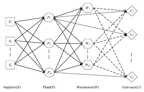
Figure 1.
Four-stage supply chain network.
Under such a four-stage supply chain network structure, the manufacturer can be viewed as a leader responsible for selecting suppliers, building manufacturing plants, and deciding the locations, capacities, and production technology of warehouses to satisfy customer demands in many customer zones. All these decisions are based on the assumption that the demand and carbon price are uncertain. A set of alternative scenarios is used to describe the uncertainties of the data. Moreover, the supply chain design must ensure stable performance over time.
In terms of sources of uncertainty, we mainly consider the uncertainty of carbon price and customer demand. The carbon price has two scenarios: low and high; the customer demand has three scenarios: low, medium, and high. In order to describe the parameters under uncertain conditions, a scenario tree is applied to describe the uncertainties. The first-stage decisions are made based on all scenarios, and the second-stage decisions are made upon the realizations of demand and carbon price. In particular, considering the lead time of production and transportation, plans and warehouses are allowed to hold appropriate inventories.
4. Model Development
Before developing the model, the following assumptions are established:
- The probability of each scenario can be set by experience and prediction;
- The specific values of uncertain parameters in different scenarios can be obtained by historical data or prediction;
- Considering the actual situation, cross-transport and multiple modes of transport are allowed. The notations used in this paper are defined and described below.
• Indices
| Supplier index, | |
| Plant index, | |
| Warehouse index, | |
| End-user index, | |
| Raw material index, | |
| Product index, | |
| Scenario index, | |
| Period index, | |
| Capacity index in a manufacturing plant, | |
| Production technology, | |
| v | Warehouse capacity level, |
| Transport mode index, | |
| End-user demand | |
| Carbon price |
• Parameters
| Market price of carbon credit in period t under scenario s | |
| Market demand of product i in period t under scenario s | |
| Maximum amount of carbon emissions allowed in period t (ton) | |
| Fixed cost of establishing plant m with technology h and capacity u | |
| Fixed cost of establishing warehouse w with capacity v | |
| Fixed cost of selecting supplier n | |
| Cost of producing a unit of product i with technology h in plant m in period t | |
| Cost of purchasing a unit of raw material r from supplier n for processing at plant m in period t | |
| Unit transportation cost for product i shipped from plant m to warehouse w through mode k in period t | |
| Unit transportation cost for product i shipped from warehouse w to end-user j through mode k in period t | |
| Unit transportation cost for product i shipped from plant m to end-user j through mode k | |
| Processing time of a unit of product i with technology h in period t (h) | |
| Volume of a unit of product i (m3) | |
| Required amount of raw material r for producing a unit of product i (kg) | |
| Production capacity (time) of plant m with technology h and capacity u (h) | |
| Holding capacity of warehouse w with capacity level v (m3) | |
| Raw material capacity of supplier n to provide raw material r in period t (kg) | |
| Per-unit storage cost of raw material r from plant m in period t | |
| Per-unit storage cost of product i from plant m in period t | |
| Per-unit storage cost of product i from warehouse w in period t | |
| Minimum inventory of raw material r from plant m in period t | |
| Minimum inventory of product i from plant m in period t | |
| Minimum inventory of product i from warehouse w in period t | |
| Safety inventory coefficient of raw material r in plant m | |
| Safety inventory coefficient of product i in plant m | |
| Safety inventory coefficient of product i in plant w | |
| Lower bound on the transfer quantity allowed from plant m to warehouse w through mode k in period t (m3) | |
| Lower bound on the transfer quantity allowed from warehouse w to end-user j through mode k in period t (m3) | |
| Lower bound on the transfer quantity allowed from plant m to end-user j through mode k in period t (m3) | |
| Upper bound on the transfer quantity allowed from plant m to warehouse w through mode k in period t (m3) | |
| Upper bound on the transfer quantity allowed from warehouse w to end-user j through mode k in period t (m3) | |
| Upper bound on the transfer quantity allowed from plant m to end-user j through mode k in period t (m3) | |
| Carbon emissions of producing a unit of product i with technology h in plant m in period t (ton) | |
| Carbon emissions of shipping a unit of product i from plant m to warehouse w through mode k in period t (ton) | |
| Carbon emissions of shipping a unit of product i from warehouse w to end-user j through mode k in period t (ton) | |
| Carbon emissions of shipping a unit of product i from plant m to end-user j through mode k in period t (ton) | |
| Unit penalty cost for the shortage of product i from end-user j in period t | |
| Probability of scenario s | |
| Total budget for establishing facilities |
• Decision variables
| If plant m with technology h and capacity u is established, , otherwise | |
| If warehouse w with capacity v, , otherwise | |
| If supplier n is selected, , otherwise | |
| If there is a flow between plant m and warehouse w though mode k in period t under scenario s, , otherwise | |
| If there is a flow between warehouse w and end-user j though mode k in period t under scenario s, , otherwise | |
| If there is a flow between plant m and end-user j though mode k in period t under scenario s, , otherwise | |
| Quantity of product i produced in plant m with technology h in time period t under scenario s | |
| The inventory of raw material r from plant m in period t under scenario s | |
| The inventory of product i from plant m in period t under scenario s | |
| The inventory of product i from warehouse w in period t under scenario s | |
| Quantity of raw material r shipped from supplier n to plant m in period t under scenario s | |
| Quantity of product i shipped from plant m to warehouse w through k in period t under scenario s | |
| Quantity of product i shipped from warehouse w to end-user j through mode k in period t under scenario s | |
| Quantity of product i shipped from plant m to end-user j through mode k in period t under scenario s | |
| Quantity of shortage for product i in end-user j in period t under scenario s | |
| Net number of carbon credits traded in period t under scenario s |
4.1. Constraints
For the supply chain network design problem, the constraints mainly include the budget constraint, the carbon credit limitation, the capacity constraint of the plants and warehouses, the material flow constraints between different supply chain participants, and the flow balances in plants and warehouses.
Constraint (1) guarantees that the total cost of establishing the manufacturing plants and warehouses should be within the budget limitation.
Constraints (2) and (3) ensure that up to one facility can be established in each candidate location.
Constraint (4) presents the carbon credit limitation for each scenario in time period t by subtracting the production and transport emissions from the regulated cap.
Constraints (5) and (6) enforce restrictions on the capacity of manufacturing plants and warehouses, respectively, in period t.
Constraint (7) ensures that no purchases are made from the unselected supplier, and limits each supplier’s capacity for supplying raw material r.
Constraint (8) ensures that the quantity of raw materials should meet the requirement of manufacturing plants.
Constraints (9), (10), and (11) enforce the flow balances in manufacturing plant, warehouse, and end-user locations, respectively.
The ending stock level of the products in the warehouse is equal to the opening stock level plus the plant-to-warehouse shipments minus the warehouse-to-customer shipments, as shown in constraint (12).
The stock level of raw materials and finished products should be no less than the required minimum stock, that is:
Constraints (16–18) prevent production interruptions due to shortage of raw materials, product. Plants and warehouses usually set the corresponding minimum inventory as a guarantee.
As stated in constraints (19–21), the transfer quantities between different supply chain participants should satisfy the product flow limitations.
Constraints (22) and (23) enforce the binary and non-negativity restrictions on decision variables.
4.2. Objective Function
In the proposed green supply chain network design model, the related costs are as follows.
The construction costs of the plant and warehouse at the beginning of the whole planning horizon are:
The costs of selecting suppliers from candidates are:
Transportation costs among plants, warehouses, and end-users in period t under scenario s are calculated as:
Production and raw materials purchasing costs in period t under scenario s are:
Penalty/shortage cost and the net cost of carbon credits in period t under scenario s are:
Inventory holding costs for raw materials, products in plants, and warehouses in period t under scenario s are calculated as:
Denote
as the total cost for the supply chain network design for scenario s during the whole period, which is given by:
4.3. Deterministic Cost Minimization Model
For any scenario s, the supply chain network design problem can be modeled as a general deterministic optimization model when the parameters are certain, that is:
For the convenience of description, let be the vector of decision variables that should be made before any scenario happens, and be the vector of control variables that can be determined after observing scenario s. Then, the above model (31) can be described as follows:
where is the feasible region defined by constraints (1)–(23) under scenario s. By solving the problem DCMs, the optimal network structure and operation strategies under any scenario s can be obtained. Since it is usually difficult to know exactly which scenarios may occur in the future, a p-robust approach is used to develop the green supply chain network design model.
4.4. p-Robust Green Supply Chain Network Design Model
For the deterministic optimization problem DCMs, let be the optimal objective function value under scenario s. Let be a feasible solution to DCMs, which corresponds to the objective function value of . For any scenario s, a relative regret value, defined as , is introduced to evaluate the robustness of a solution. Let represent the relative regret limit, for a given value, if is valid for all scenarios, the feasible solution is considered as a p-robust solution, because the relative regret value is not higher than the desired level [24]. Then, we develop the following p-robust green supply chain network design model (RSCND):
where the objective function measures the expected total cost for the supply chain network design. Let be the optimal solution of RSCND model; constraint (32) measures the robustness of a solution in any scenario. In many studies, the value of the relative regret limit p is assumed to be arbitrary. However, it can be seen that there may exist many feasible, robust solutions satisfying constraint (32) if p is large enough; conversely, there may be no feasible, robust solutions if p is too small. Therefore, in order to obtain the optimal robust solution, we will introduce an approach to determine the lower bound and upper bound of the p values in the next section. The decision-maker can adjust the robustness level of the designed supply chain network by dynamically adjusting the relative regret limit p.
4.5. Determine Upper and Lower Bounds for Relative Regret Limit
In order to ensure the existence of a feasible solution to the RSCND model, the relative regret limit p cannot be infinitesimally. Therefore, it is needed to determine a lower bound for the relative regret limit, which is noted as . When , the relative regret for the worst-case scenario reaches the lowest level, thus obtaining the optimal network design scheme in the worst case. Even in the worst case, constraint (32) needs to be satisfied. However, the expected total cost will be higher due to the small feasible solution region. On the other hand, the expected total cost in RSCND decreases with the increases of the relative regret limit because of the increasing of the feasible solution region. In particular, when the relative regret limit p is very large, constraint (32) in RSCND becomes a redundant constraint, resulting in RSCND becoming a general stochastic programming model without constraint (32). Therefore, it is necessary to set an upper bound
for the relative regret limit, which can be defined as the smallest relative regret limit that enables the expected total cost in RSCND to reach its same minimum value as without constraint (32) in RSCND.
A larger relative regret limit corresponds to a smaller expected total cost, but the supply chain network has inferior robustness in dealing with uncertain disturbances. Therefore, there is a tradeoff between the overall performance and the worst-case performance. When selecting a small relative regret limit, the solution benefits the worst-case scenario, but damages the performance of the supply chain network, and vice versa. The value of the relative regret limit p can be selected according to the supply chain network designer’s preference. If the risk-averse designer prefers to pursue good performance for the worst-case scenario, it is better to select a smaller relative regret limit. On the contrary, if the designer is willing to pursue the optimal performance for all scenarios and is able to bear the worst-case performance, then it is better to select a larger relative regret limit. In the following, the method to obtain lower bound and upper bound are presented.
The lower bound is the smallest value that guarantees the existence of a feasible solution to the problem RSCND. Thereby, it can be obtained by solving the following model (p-LOW):
According to problem RSCND, when the relative regret limit p is large enough, constraint (32) becomes redundant, and the objective function reduces to its minimum value , which can be obtained by solving the following stochastic programming model (SPM):
On that basis, the upper bound can be obtained by solving the following model (p-UP) with an extra constraint, :
By solving the above p-LOW, SPM, and p-UP models, the lower bound and upper bound can be obtained. Any value of can be used to solve model RSCND, and then obtain a robust green supply chain network design scheme. Note that all modes including p-LOW, SPM, p-UP, and RSCND are mixed integer linear programming, which can be solved efficiently.
5. Scenario Generation and Reduction
This study considers two sources of uncertainty: carbon price and market demand. A scenario tree approach is applied to describe the uncertainties in both sources. Let denote the carbon price, which has two possible values, and , representing low and high prices, respectively, . In each period t, the corresponding probabilities that the carbon price scenarios occur are and , . Let D denote the future market demand, which has three possible values, D1, D2, and D3, representing low, medium, and high demand, respectively, . The corresponding probabilities that the demand scenarios occur in period t are , , and , . Then, the total number of scenarios for the whole period is calculated as , and the probability that each scenario s happens is . As can be seen from Figure 2, the number of uncertain scenarios will increase exponentially with the increase of the number of periods, which results in too large a model to be solved effectively. Then, we introduce a scenario reduction technique to filter the scenarios, which reduces the solving difficulty.
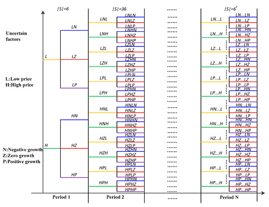
Figure 2.
Scenario tree.
In a multi-scenario problem, let be the vector of uncertain parameters. Let the uncertain parameter take on a finite set of values given by . The probability associated with the uncertain parameter taking on a value is , . To model the selection of scenarios, let the new probability assigned to a scenario s be , a continuous variable. The scenario reduction optimization model can be described as in reference [32]:
By solving model (33), the minimum set of scenarios and their associated probabilities are obtained. Denote as the value of the probability corresponding to scenario s with the uncertain parameters in the reduced set of scenarios.
6. Numerical Studies
6.1. Description and Parameter Assignment
In order to verify the validity of the proposed p-robust green supply chain network design model, numerical calculations are carried out for the automotive components’ supply chain network design. Due to confidentiality, the true data in a real case cannot be accessed unconditionally. Therefore, a virtual case study is created to perform the experiment, in which a set of representative data is presented. During the planning period , plants use raw materials to produce products with a ratio of and volume of to meet the demand of end-user areas. We assume that there are potential suppliers and the supply capacities are 6000, 6500, and 7000 for each one. Further, potential plants use two optional technologies to make products, and the products are shipped out from the plant through a series of optional paths to the warehouse or directly to the end user. The capacity for each manufacturing plant can be small, medium, or large, denoted as , , and , respectively, in which . After arriving at the warehouse, the products are allocated and sorted in order to deliver the products to the customer area accurately and in a timely manner. The minimum transport volumes from plant to warehouse, warehouse to end user, and plant to end user are all set as 0, and the maximum transport volumes are set as 4000, 4000, and 1000, respectively. The carbon emissions per unit product of transport from plant to warehouse, warehouse to end user, and plant to end user are set as 0.5, 0.8, and 4, respectively. The safety inventory coefficients of raw materials and products in factories are and , respectively. There are potential warehouses, and the safety inventory coefficient of products in each warehouse is set as . We assume that the total budget for the establishment of facilities does not exceed 170,000. Other parameters, such as requirements and costs required for the model, are shown in Table 1, Table 2, Table 3, Table 4, Table 5, Table 6, Table 7, Table 8, Table 9, Table 10, Table 11 and Table 12.

Table 1.
End-user demand for products and unit penalty cost.
Table 2.
Maximum overall allowed carbon emissions and price of carbon credit.
Table 3.
Fixed cost of establishing plant m with technology h and capacity u.
Table 4.
Processing time per unit product with technology h.
Table 5.
Production capacity (time) in plant m with technology h and capacity u.
Table 6.
Fixed cost of establishing warehouse with a certain capacity.
Table 7.
Cost of manufacturing a unit product and estimated carbon emissions to produce a unit product.
Table 8.
Fixed cost of selecting supplier and unit purchasing cost of raw material.
Table 9.
Unit transportation cost for product shipped from plant to warehouse and end user.
Table 10.
Unit transportation cost for product shipped from warehouse to end user.
Table 11.
Per-unit storage cost of product and raw material.
Table 12.
Carbon price and demand scenario probability in different periods after scenario reduction.
In each period t, the probabilities of two price scenarios (low and high) are set to and , respectively. Furthermore, the probabilities of three demand scenarios (low, zero, and high), , , and , are used. Thus, we have six combinatorial scenarios altogether, and the corresponding probabilities are , , , , , and . By solving model (33), 11 scenarios and their corresponding probabilities are obtained, as shown in Table 12. All the models, including DCMs, p-LOW, SPM, p-UP, and RSCND, are coded in GAMS 24.7.1 modeling language using CPLEX as the core optimization solver.
6.2. Results Analysis
1. Total costs of supply chain network in different scenarios.
In this section, we evaluate the performance of the proposed p-robust green supply chain network design model under different scenarios. By solving p-LOW, SPM, and p-UP, the lower and upper bounds as well as the minimum expected total cost are obtained as , , and , respectively. Besides, the problem DCMs is solved for determining the optimal cost under different scenarios (see second column in Table 13). Likewise, the robust optimal costs under the 11 scenarios are also calculated by solving the p-robust model RSCND for the resulting lower and upper bounds. In order to verify the robustness of the proposed approach, the relative regret value is further calculated under different scenarios.
Table 13.
Objective function and relative regret for each scenario.
The results in Table 13 show that under the same scenario s, the robust optimal costs are higher than the deterministic supply chain network design costs both for the lower and upper bounds. This increasing trend is due to the uncertainty of carbon price and demand, but the increasing proportion is small. For example, the largest relative regret values are 0.0323 for the lower bound and 0.0418 for the upper bound, both in scenario 4. Since the relative regret values are somewhat small, decision-makers can effectively use the proposed p-robust optimization approach to deal with carbon and demand uncertainties, which shows that the proposed model is robust.
As can be seen from Table 13, compared with the total cost of a deterministic supply chain network design under a single scenario, the total cost of the network under any scenario obtained by solving the p-robust model RSCND in this paper shows an increasing trend due to the uncertainty of carbon price and demand, but the increasing proportion is small, which shows that the proposed model is robust.
2. Expected value of perfect information (EVPI).
The EVPI is defined as the difference between and [33]. Thus, the value of EVPI in this study is , which can be interpreted as a fee that a decision-maker is willing to pay to gain access to perfect carbon price and customer demand information.
3. Performance comparisons and carbon emission comparisons under robust optimization and stochastic programming.
To highlight the advantages of the proposed approach in dealing with carbon price and customer demand uncertainties, a comparative performance evaluation is conducted first for the robust optimization model with and the stochastic programming model (SPM). Denote and as their corresponding optimal costs under different scenarios, and the relative regret limit p is set as . In addition, let , and be the relative ratios expressed as , , and , respectively, to reflect the magnitude of cost fluctuations because of carbon price and customer demand uncertainties. As shown in Table 14, the largest relative ratios are 3.23% for and 4.18% for . The smallest relative ratios are 2.90% for and 0.07% for , respectively. These experimental results demonstrate that the cost fluctuation induced by the robust optimization model is smaller than that induced by the stochastic programming model, indicating that the proposed p-robust green supply chain network design model can better hedge against the carbon price and demand uncertainties, and achieve a more stable cost performance.
Table 14.
Performance comparisons under robust optimization and stochastic programming.
From Table 14, it can be seen that the maximum value of robust optimization is 3.23%, and the minimum value is 2.90%. The maximum value of stochastic programming is 4.18%, and the minimum value is 0.07%. In conclusion, the fluctuation of the objective function value of robust optimization is relatively small, whereas that of stochastic programming is relatively large. This shows that the p-robust green supply chain network design method can achieve more stable cost performance under uncertain carbon price and demand.
Further analysis is performed to study the impact of carbon price and demand uncertainties on carbon emissions. Let represent the optimal carbon emission under scenario s. Denote and as the carbon emissions derived by robust optimization with and stochastic programming, respectively. Similarly, let , and be the relative ratios expressed as , , and , respectively. Table 15 shows that the absolute value of is less than or equal to that of in any scenario s, which further provides evidence that the proposed p-robust green supply chain network design model can better hedge against the carbon price and demand uncertainties and achieve more stable solutions.
Table 15.
Carbon emissions derived by robust optimization and stochastic programming.
4. Cost performance and carbon emission evaluations under different p values.
More experiments are conducted to investigate the impact of the relative regret limit p on the supply chain network cost performance, carbon emission cost, and carbon emission. In order to observe the changing tendencies of the cost–profit performances and the carbon emissions, the relative regret limit p is set to start from the lower bound to the upper bound in increments of . By solving RSCND, we obtain the results shown in Figure 3 and Figure 4. Figure 3 shows that when p is small enough, the robustness of the supply chain network is better, whereas the expected total cost is higher, and vice versa. Therefore, it is necessary to make a tradeoff between p and the total cost of the supply chain network system. As shown in Figure 3, there are three effective design schemes: when p is set as , , and , the supply chain network costs are , , and , respectively. These results imply that, from the perspective of supply chain cost performance stability, risk-averse decision-makers should choose the scheme with a lower p, whereas risk-preference decision-makers should choose the scheme with a larger p to save costs.
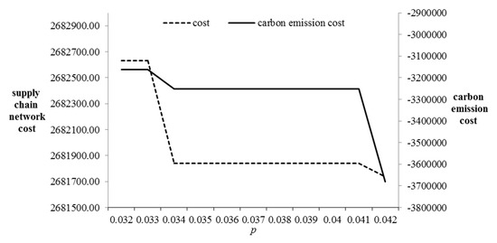
Figure 3.
Total network cost and carbon emission cost under different relative regret limits.
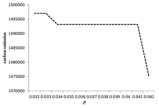
Figure 4.
Carbon emissions under different relative regret limits.
From Figure 3 and Figure 4, it can be seen that both the carbon emission cost and the carbon emission decrease as p increases, which means that decision-makers can achieve substantial emission reductions by increasing p slightly. That is, environmentalists tend to choose the scheme with a larger relative regret limit p.
5. Supply chain network structure.
According to the three effective design schemes derived above and the two-stage stochastic programming design scheme, the corresponding supply chain network structures are given in Figure 5, Figure 6, Figure 7 and Figure 8, where the figures above facilities represent the outputs of products, the figures below facilities represent the inventory level of products, and the figures between facilities represent the volume of raw materials transported and the distribution of products. The results in Figure 5, Figure 6, Figure 7 and Figure 8 show that when , the optimal supply chain network node selection scheme includes the suppliers , , and , the plants and , and the warehouses and (see Figure 5). From Figure 6, Figure 7 and Figure 8, we can see that the supply chain network structures for three situations (, , and stochastic programming) are the same, and the optimal choice is , , , , , , and .
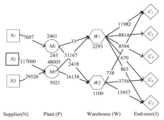
Figure 5.
Supply chain network structure when .
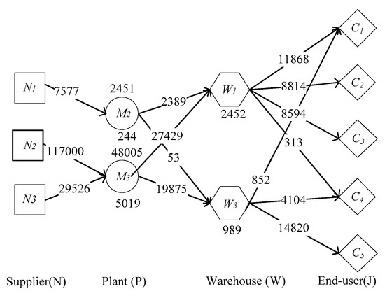
Figure 6.
Supply chain network structure when .
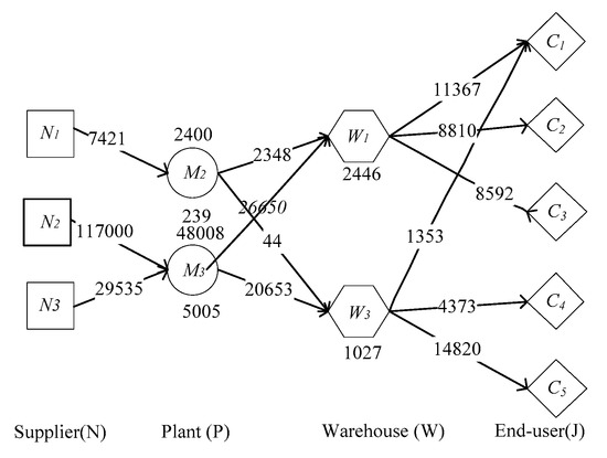
Figure 7.
Supply chain network structure when .
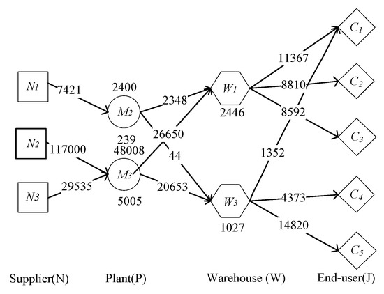
Figure 8.
Supply chain network structure by stochastic programming model (SPM).
Figure 5, Figure 6, Figure 7 and Figure 8 show that only when the regret value limit p is set as the lower bound (), the design of the supply chain network is different in node selection, which is mainly reflected in the warehouse selection (the warehouse selection is and for the case , whereas the warehouse selection is and for other cases). In the case where , the robustness level of the supply chain network as well as the corresponding total network cost are the highest. With the increase of p, the network structure remains unchanged, but the level of robustness and the total cost of the network decrease. However, it can be seen from the transportation path and quantity distribution that there are obvious differences in the second-stage decision making corresponding to the four network structures. The results show that the supply chain network designed according to the proposed p-robust approach has good stability in its structure.
7. Conclusions
In this research, we provided an approach for designing a robust green supply chain network with uncertain carbon price and market demand. Under the constraints of supply chain network structure, logistics operation, carbon emission, inventory, and cost, a two-stage SPM and a scenario-based multi-product, multi-period green supply chain network model based on p-robustness in a carbon trading environment were developed. For the p-robust green supply chain network problem, the solution method for determining the lower and upper bounds of the relative regret limit was proposed, which is convenient for decision-makers in choosing the corresponding supply chain network structure through the tradeoff between risk and cost performance. A scenario tree was applied to describe uncertainties in both carbon price and market demand, and the number of uncertain scenarios tended to increase exponentially with the increase of the number of periods, which resulted in too large a model to be solved effectively. Thus, a scenario reduction technique was proposed to filter the scenarios and maintain the validity of the results.
Numerical experiments were conducted to validate the effectiveness and practicality of the proposed p-robust optimization approach in coping with carbon price and demand uncertainties. The results show that the proposed p-robust green supply chain network design model can effectively hedge against the demand and carbon price uncertainties, and provide more options for decision-makers with different risk preferences. Especially, the total network cost fluctuation induced by the robust optimization model is smaller than that induced by the stochastic programming model, indicating that the proposed p-robust green supply chain network design model can achieve a more stable cost performance. A risk-averse decision-maker should choose the scheme with a lower relative regret limit, whereas a risk-taking decision-maker should choose the scheme with a larger relative regret limit to save costs. If companies use the proposed p-robust optimization approach to design their green supply chain network in the initial stages, they might reduce the potential marketing risks, substantially reduce the redesign costs, and effectively hedge against uncertainty disturbances. Moreover, the carbon emission cost and carbon emission decreased with the increase of p, indicating that selling carbon quota can benefit enterprises and reduce carbon emissions, so as to achieve the goal of energy conservation and emission reduction.
Our models can be extended to multi-period cases involving a consideration of the uncertainty of the emissions rate of production systems. Furthermore, risk measures, such as mean–variance and conditional risk, can also be used to measure the cost–performance risk of the supply chain network. Another interesting direction for future research is to construct the uncertainty sets of carbon price and demand to study the green supply chain network design problem under the criterion of minimum–maximum or minimum–maximum regret values. Finally, designing a green supply chain network under different carbon price policies or demand uncertainty may also be future research directions.
Author Contributions
R.Q. and S.S. developed the model and wrote the paper. All authors read and improved the final manuscript.
Funding
This research received no external funding.
Acknowledgments
The authors acknowledge support from the National Nature Science Foundation of China (No. 71772035), the Innovation Talent Funds of Liaoning Province (WR2017003), and the Fundamental Research Funds for the Central Universities (N180614003).
Conflicts of Interest
The authors declare no conflict of interest.
References
- Waltho, C.; Elhedhli, S.; Gzara, F. Green supply chain network design: A review focused on policy adoption and emission quantification. Int. J. Prod. Econ. 2019, 208, 305–318. [Google Scholar] [CrossRef]
- Xu, X.; Wei, Z.; Ji, Q.; Wang, C.; Gao, G. Global renewable energy development: Influencing factors, trend predictions and countermeasures. Resour. Policy 2019, 63, 101470. [Google Scholar] [CrossRef]
- Dehghanian, F.; Mansour, S. Designing sustainable recovery network of end-of-life products using genetic algorithm. Resour. Conserv. Recycl. 2009, 53, 559–570. [Google Scholar] [CrossRef]
- Wang, G.; Gunasekaran, A.; Ngai, E.W.T. Distribution network design with big data: Model and analysis. Ann. Oper. Res. 2018, 270, 539–551. [Google Scholar] [CrossRef]
- Govindan, K.; Fattahi, M.; Keyvanshokooh, E. Supply chain network design under uncertainty: A comprehensive review and future research. Eur. J. Oper. Res. 2017, 263, 108–141. [Google Scholar] [CrossRef]
- Rezaee, A.; Dehghanian, F.; Fahimnia, B.; Beamon, B. Green supply chain network design with stochastic demand and carbon price. Ann. Oper. Res. 2017, 250, 463–485. [Google Scholar] [CrossRef]
- Zakeri, A.; Dehghanian, F.; Fahimnia, B.; Sarkis, J. Carbon pricing versus emissions trading: A supply chain planning perspective. Int. J. Prod. Econ. 2015, 164, 197–205. [Google Scholar] [CrossRef]
- Gao, N.; Ryan, S.M. Robust design of a closed-loop supply chain network for uncertain carbon regulations and random product flows. EURO J. Transp. Logist. 2014, 3, 5–34. [Google Scholar] [CrossRef]
- Mohammed, F.; Selim, S.Z.; Hassan, A.; Syed, M.N. Multi-period planning of closed-loop supply chain with carbon policies under uncertainty. Transp. Res. Part D Transp. Environ. 2017, 51, 146–172. [Google Scholar] [CrossRef]
- Elhedhli, S.; Merrick, R. Green supply chain network design to reduce carbon emissions. Transp. Res. Part D Transp. Environ. 2012, 17, 370–379. [Google Scholar] [CrossRef]
- Jin, M.; Granda-Marulanda, N.A.; Down, I. The impact of carbon policies on supply chain design and logistics of a major retailer. J. Clean. Prod. 2014, 85, 453–461. [Google Scholar] [CrossRef]
- Fareeduddin, M.; Hassan, A.; Syed, M.; Selim, S. The impact of carbon policies on closed-loop supply chain network design. Procedia CIRP 2015, 26, 335–340. [Google Scholar] [CrossRef]
- Fahimnia, B.; Sarkis, J.; Choudhary, A.; Eshragh, A. Tactical supply chain planning under a carbon tax policy scheme: A case study. Int. J. Prod. Econ. 2015, 164, 206–215. [Google Scholar] [CrossRef]
- Xu, Z.; Pokharel, S.; Elomri, A.; Mutlu, F. Emission policies and their analysis for the design of hybrid and dedicated closed-loop supply chains. J. Clean. Prod. 2017, 142, 4152–4168. [Google Scholar] [CrossRef]
- Kuo, T.C.; Lee, Y. Using pareto optimization to support supply chain network design within environmental footprint impact assessment. Sustainability 2019, 11, 452. [Google Scholar] [CrossRef]
- Alkhayyal, B. Corporate social responsibility practices in the U.S.: Using reverse supply chain network design and optimization considering carbon cost. Sustainability 2019, 11, 2097. [Google Scholar] [CrossRef]
- Xu, X.; Hao, J.; Yu, L.; Deng, Y. Fuzzy optimal allocation model for task-resource assignment problem in collaborative logistics network. IEEE Trans. Fuzzy Syst. 2019, 27, 1112–1125. [Google Scholar] [CrossRef]
- Zeballos, L.J.; Méndez, C.A.; Barbosa-Povoa, A.P.; Novais, A.Q. Multi-period design and planning of closed-loop supply chains with uncertain supply and demand. Comput. Chem. Eng. 2014, 66, 151–164. [Google Scholar] [CrossRef]
- Ayvaz, B.; Bolat, B.; Aydın, N. Stochastic reverse logistics network design for waste of electrical and electronic equipment. Resour. Conserv. Recycl. 2015, 104, 391–404. [Google Scholar] [CrossRef]
- Zhou, X.; Zhang, H.; Qiu, R.; Lv, M.; Xiang, C.; Long, Y.; Liang, Y. A two-stage stochastic programming model for the optimal planning of a coal-to-liquids supply chain under demand uncertainty. J. Clean. Prod. 2019, 228, 10–28. [Google Scholar] [CrossRef]
- Pishvaee, M.S.; Rabbani, M.; Torabi, S.A. A robust optimization approach to closed-loop supply chain network design under uncertainty. Appl. Math. Model. 2011, 35, 637–649. [Google Scholar] [CrossRef]
- Ramezani, M.; Bashiri, M.; Tavakkoli-Moghaddam, R. A robust design for a closed-loop supply chain network under an uncertain environment. Int. J. Adv. Manuf. Tech. 2013, 66, 825–843. [Google Scholar] [CrossRef]
- Baghalian, A.; Rezapour, S.; Farahani, R.Z. Robust supply chain network design with service level against disruptions and demand uncertainties: A real-life case. Eur. J. Oper. Res. 2013, 227, 199–215. [Google Scholar] [CrossRef]
- Tian, J.; Yue, J. Bounds of relative regret limit in p-robust supply chain network design. Prod. Oper. Manag. 2014, 23, 1811–1831. [Google Scholar] [CrossRef]
- Niknamfar, A.H.; Niaki, S.T.A.; Pasandideh, S.H.R. Robust optimization approach for an aggregate production–distribution planning in a three-level supply chain. Int. J. Adv. Manuf. Tech. 2015, 76, 623–634. [Google Scholar] [CrossRef]
- Akbari, A.A.; Karimi, B. A new robust optimization approach for integrated multi-echelon, multi-product, multi-period supply chain network design under process uncertainty. Int. J. Adv. Manuf. Tech. 2015, 79, 229–244. [Google Scholar] [CrossRef]
- Hasani, A.; Zegordi, S.H.; Nikbakhsh, E. Robust closed-loop global supply chain network design under uncertainty: The case of the medical device industry. Int. J. Prod. Res. 2015, 53, 1596–1624. [Google Scholar] [CrossRef]
- Marufuzzaman, M.; Eksioglu, S.D.; Huang, Y. Two-stage stochastic programming supply chain model for biodiesel production via wastewater treatment. Comput. Oper. Res. 2014, 49, 1–17. [Google Scholar] [CrossRef]
- Nickel, S.; Saldanha-da-Gama, F.; Ziegler, H.P. A multi-stage stochastic supply network design problem with financial decisions and risk management. Omega 2012, 40, 511–524. [Google Scholar] [CrossRef]
- Pimentel, B.S.; Mateus, G.R.; Almeida, F.A. Stochastic capacity planning and dynamic network design. Int. J. Prod. Econ. 2013, 145, 139–149. [Google Scholar] [CrossRef]
- Fattahi, M.; Govindan, K.; Keyvanshokooh, E. Responsive and resilient supply chain network design under operational and disruption risks with delivery lead-time sensitive customers. Transp. Res. Part E Logist. Transp. Rev. 2017, 101, 176–200. [Google Scholar] [CrossRef]
- Karuppiah, R.; Martín, M.; Grossmann, I.E. A simple heuristic for reducing the number of scenarios in two-stage stochastic programming. Comput. Chem. Eng. 2010, 34, 1246–1255. [Google Scholar] [CrossRef]
- Birge, J.R.; Louveaux, F. Introduction to Stochastic Programming; Springer: Berlin/Heidelberg, Germany, 1997. [Google Scholar]
© 2019 by the authors. Licensee MDPI, Basel, Switzerland. This article is an open access article distributed under the terms and conditions of the Creative Commons Attribution (CC BY) license (http://creativecommons.org/licenses/by/4.0/).