Real-Time Prediction of the Rheological Properties of Water-Based Drill-In Fluid Using Artificial Neural Networks

Abstract

The rheological properties of drilling fluids are the key parameter for optimizing drilling operation and reducing total drilling cost by avoiding common problems such as hole cleaning, pipe sticking, loss of circulation, and well control. The conventional method of measuring the rheological properties are time-consuming and require a high effort for equipment cleaning, so they are only measured twice a day. There is a need to develop an automated system to measure the rheological properties in real-time based on the frequent measurements of mud density, Marsh funnel time, and solid percent. The main objective of this paper is to apply a modified self-adaptive differential evolution technique to determine the optimum combination of an artificial neural network’s variables to precisely predict the rheological properties of water-based drill-in fluid using the frequent measuring of mud density, Marsh funnel time, and solid percent. The second objective is whitening the black box of an artificial neural network by developing five new empirical correlations to determine the rheological properties without the need for the artificial neural network models. Actual field measurements (900 data points) were used to train, test, and validate the artificial neural network models and the developed empirical correlations. The optimization process illustrated that the best training function was Bayesian regularization backpropagation (trainbr), and the best transferring function was Elliot symmetric sigmoid (elliotsig). The optimum number of neurons was 30 for the plastic viscosity and the flow consistency index, while it was 29 for apparent viscosity, yield point, and the flow behavior index. The developed artificial neural network models and empirical correlations predicted the rheological properties with high accuracy. The correlation coefficient (R) was more than 90%, and the average absolute percentage error was less than 8.6%. The new technique for rheological properties estimation is an example of the new development which will help the new generation to discover and extract oil and gas with less cost and with safer operations.

1. Introduction

Water-based drill-in fluid (WBDIF) is used to drill the reservoir section, which carries the hydrocarbon. WBDIF should be designed to be non-damaging by building an impermeable layer on the face of the formation during the drilling process while this layer should be removed easily before casing and cementing the hole. WBDIF should provide stable rheological properties (RHPs) in order to provide a stable and clean hole and to prevent cutting accumulation, both of which lead to the possibility of pipe sticking, [1,2,3]. The main function of WBDIF is to support formation pressure and prevent reservoir fluid from entering the wellbore while drilling [4]. In addition, the drill-in fluid should cool and lubricate the bit and the drill string [5,6].

Sodium chloride-water-based drill-in fluid (NaCl-WBDIF) is mainly used while drilling the reservoir section. NaCl salt is used as a weighting material to increase mud density, while the Na+ ions work as shale stabilizers [7]. NaCl polymer mud is characterized as an inhibited, non-dispersed drilling fluid in which the viscosity control and the filtration properties are enhanced by using some types of polymers such as xanthan gum and starch. This helps reduce the possibility of formation damage [8].

RHPs play a key role in the success of the drilling operation. RHPs such as plastic viscosity (PV), yield point (YP), apparent viscosity (AV), flow consistency index (K), and flow behavior index (n) should be determined in real-time to calculate rig hydraulics and determine the required pressure to optimize hole cleaning. Increasing the PV value gives an indication about the increase in solid content, and it can highly affect the rate of penetration [9,10,11]. Paiaman et al. [12] stated that a lower YP value is preferred in turbulent flow, while a high YP value is required for laminar flow. The ratio of YP/PV is very important for hole cleaning. The YP/PV ratio should be greater than 1.5 [13]. The consistency index of the drilling fluid (k) is the main controlling parameter of the carrying capacity index (CCI) [14].

The common procedure in rig-sites is that the drilling crew usually measures the mud density and Marsh funnel time [15] every 15–20 min, and these measurements are used as indicators for the changes in the fluid properties [16]. Other RHPs (PV, YP, n, and K) are usually measured twice a day, as it requires a long time to heat the fluid, record, analyze the data, and clean the equipment. This process is tedious and time-consuming.

The effect of solid content on drilling fluid RHPs is very obvious, as can be seen throughout the literature. The objective of this study was to develop novel empirical models that are capable of acquiring the RHPs of NaCl polymer mud using one of the powerful artificial intelligence techniques—the artificial neural network (ANN)—using 900 field measurements of mud density (MD), Marsh funnel time (FT), and solid percent (SP). The novelty of this research is getting a real-time prediction (every 10–15 min) of the mud RHPs. Additionally, in this paper, a self-adaptive evolution algorithm was used to optimize the input parameters at the same time, and this was linked with the ANN model. The developed method depends on taking the reading from the automated Marsh funnel system (which contains different sensors) and applying artificial neural network models to predict the rheological properties every 10–20 min, which enable the driller to understand the changes of the drilling fluid properties as well as changes in the rig hydraulics. This make decisions regarding the required action based on given information much faster.

Artificial Neural Network

The concept of artificial networks was introduced into engineering research in the 1940s [17,18]. At early stages, artificial intelligence (AI) was used to solve the complex equations and mimic the nervous system [19,20].

The ANN has been considered as an effective AI tool; therefore, it has been widely applied in several fields such as classification and optimization tasks [21,22]. The ANN model is a system of neurons and hidden layers [23]. Usually, the whole data are grouped into two sets—training and testing data sets. The training group is used to train the network and capture the relationship between the input and output parameters, while the testing data are used to measure the reliability of the developed ANN system. During the training stage, the testing data remain unseen by the model, which provides more confidence regarding model reliability [24,25,26].

Alajmi et al. [27] predicted choke performance using an ANN. Alarifi et al. [28] estimated the productivity index for oil horizontal wells using an ANN, a functional network and fuzzy logic. Chen et al. [29] applied a NN and fuzzy logic to evaluate the performance of an inflow control device (ICD) in a horizontal well. Their model investigated the influences of reservoir parameters (such as reservoir size, thickness, reservoir heterogeneity, and permeability ratio) on ICD completion performance. Van and Chon [30,31] evaluated the performance of carbon dioxide (CO₂) flooding using ANN techniques. They developed ANN models for determining oil production rate, CO₂ production, and gas-oil ratio (GOR).

The self-adaptive differential evolution (SaDE) was introduced by Qin et al. [32] to overcome the common issues of the differential evaluation (DE) [33]. The advantage of the SaDE is the ability to self-adapt the controlling parameters and mutation strategies based on the learning experience in the previous algorithm generations to obtain better results. Moussa and Awotunde [34] developed a modified SaDE that can be used for the optimization in different engineering problems.

Al-Khdheeawi and Mahdi [35] applied an ANN to predict the apparent viscosity of water-based drilling fluid using the mud density and Marsh funnel time. They concluded that the developed ANN correlation could predict AV with an average absolute percentage error (AAPE) of 8.6% and a correlation coefficient of 98.8%. Gowida et al. [36] stated that the ANN can be used efficiently to predict the rheological properties of the calcium chloride (CaCl₂) water-based drilling fluid based on mud density and Marsh funnel time.

Zhang et al. [37] developed a new technique for breast cancer detection using a combination of rectified linear unit and rank-based stochastic pooling. They concluded that the detection efficiency of the new technique overcomes the known six standard techniques known for breast cancer detection. For abnormal breasts in mammogram images, Wang et al. [38] developed a combined system of a feed-forward neural network with principal computer analysis, a Jaya algorithm, and a weighted-type fractional Fourier transform. They concluded that Jaya was a better algorithm for training the feed-forward neural network than the common know algorithms, and the developed technique was able to detect the abnormal breast with high accuracy (>92.27%).

The main goal of this study was to develop new sets of empirical correlations, optimized using modified self-adaptive differential evolution (MSaDE), to determine the RHPs of NaCl-WBDIF using a hybrid ANN model.

2. Methodology

ANN variables such as percent of training to testing, number of neurons, training and testing functions, and the number of layers should be optimized to develop a robust ANN model, and from this model, empirical correlation can be extracted. In this study, MSaDE was applied to optimize the variable parameters of the ANN for different RHPs. Nine-hundred field measurements were used to train, test, and validate the ANN models. The data were selected randomly to train the model, with 65% of the data being used for training (570 data points), 23% of the data being used for testing (180 data points), and 12% of the data being used (150 data points) for further validation. The ANN models were built using 88% of the available data, including training and testing and based on the optimized models, and the new empirical correlation was developed. The 12% remaining of data were used to validate the developed empirical correlations. The correlation coefficient ^®, AAPE, and visualization check were used as criteria to evaluate the developed models and correlations.

The AAPE is a measure of the relative deviation of the predicted data from the real data and can be calculated using Equation (1):

$$\mathrm{AAPE}=\frac{1}{\mathrm{n}}{\displaystyle \sum }_{\mathrm{i}=1}^{\mathrm{n}}\left|{\mathrm{E}}_{\mathrm{i}}\right|$$

(1)

where n is the number of data points and E_i is the relative deviation of a predicted value from a real value, Equation (2);

$${\mathrm{E}}_{\mathrm{i}}=\left(\frac{{\mathrm{y}}_{\mathrm{real}}-{\mathrm{y}}_{\mathrm{predict}}}{{\mathrm{y}}_{\mathrm{real}}}\right)\ast 100$$

(2)

For the network training and transferring functions, two pools of 12 different training functions and 7 transferring functions were established, respectively. Each individual training/transferring function was indexed and used as one of the input parameters to the MSaDE optimization algorithm along with the other parameters such as the number of neurons, the percent of training to testing, and the number of hidden layers. Twenty independent optimization runs were performed to optimize the above-mentioned parameters. The optimization run that resulted best fit (in terms of the highest R and the lowest AAPE was considered as the best run, and its results are shown and discussed in this paper.

Data Description

Data were collected from different wells which were drilled using NaCl-WBDIF. Nine-hundred data records of MD, FT, SP, PV, and YP were used to train, test and validate the developed correlations for different RHPs. The data were collected while drilling a different reservoir section in which non-damaging drill-in fluid was used. The rheological properties were measure twice a day, and the mud density, solid percent and Marsh funnel time were measured at the same time.

Table 1 lists the statistical parameters of the nine-hundred data points. The drill-in fluid covered a wide range of fluid density where the MD ranged from 64 to 121 ppg. The FT ranged from 35 to 91 s/quart, and SP ranged from 0 to 32.5%. PV ranged from 7 to 51 cP, and the YP ranged from 19 to 45 lb/100 ft². Figure 1 shows that the PV was a strong function of MD and SP, where the R was 0.76 and 0.70 for MD and SP, respectively. PV was a moderate function of FT, with its R being 0.57. YP was a strong function of MD and moderate function of SP and FT. The R was 0.67, 0.58, and 0.42 for MD, SP, and FT, respectively, as seen in Figure 1.

Table 1. Statistical analysis of the collected field data from the drill-in fluid.

Statistical Parameter	Mud Weight (MD)	Marsh Funnel Time (MT)	Solid Percent (SP)	Plastic Viscosity (PV)	Yield Point (YP)
Minimum	64	35	0	7	19
Maximum	121	91	32.5	51	45
Mean	82.12	59.22	13.79	21.65	27.15
Median	78	58	13	20	27
Standard Deviation	14.33	10.10	7.18	8.15	3.95
Kurtosis	0.50	0.20	−0.39	0.74	1.23
Skewness	1.08	0.59	0.44	0.91	0.87

Figure 1. The relative importance of the input parameters to plastic viscosity and yield point.

3. Results and Discussion

3.1. Building Artificial Intelligence Models

The MSaDE technique was applied to optimize the ANN model for the PV. Equations (3)–(6) were used to normalize the input and the output parameters for the model. To train the ANN model, 570 data points were used.

$${\mathrm{MD}}_{\mathrm{n}}=0.034\ast \left(\mathrm{MD}-64\right)-1$$

(3)

$${\mathrm{FT}}_{\mathrm{n}}=0.036\ast \left(\mathrm{FT}-35\right)-1$$

(4)

$${\mathrm{SP}}_{\mathrm{n}}=0.062\ast \mathrm{SP}-1$$

(5)

$${\mathrm{PV}}_{\mathrm{n}}=0.044\ast \left(\mathrm{PV}-6\right)-1$$

(6)

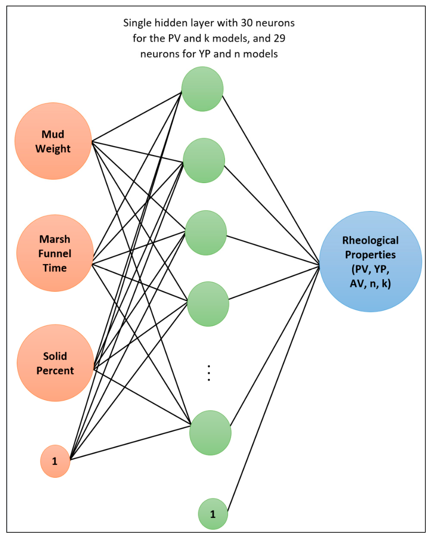
The optimization process showed that the best training function was Bayesian regularization backpropagation (trainbr) when using three input parameters (MD, FT, SP), and the optimized number of neurons was 30 when only one hidden layer was applied. The optimization process showed that the best transferring function was Elliot symmetric sigmoid (elliotsig).

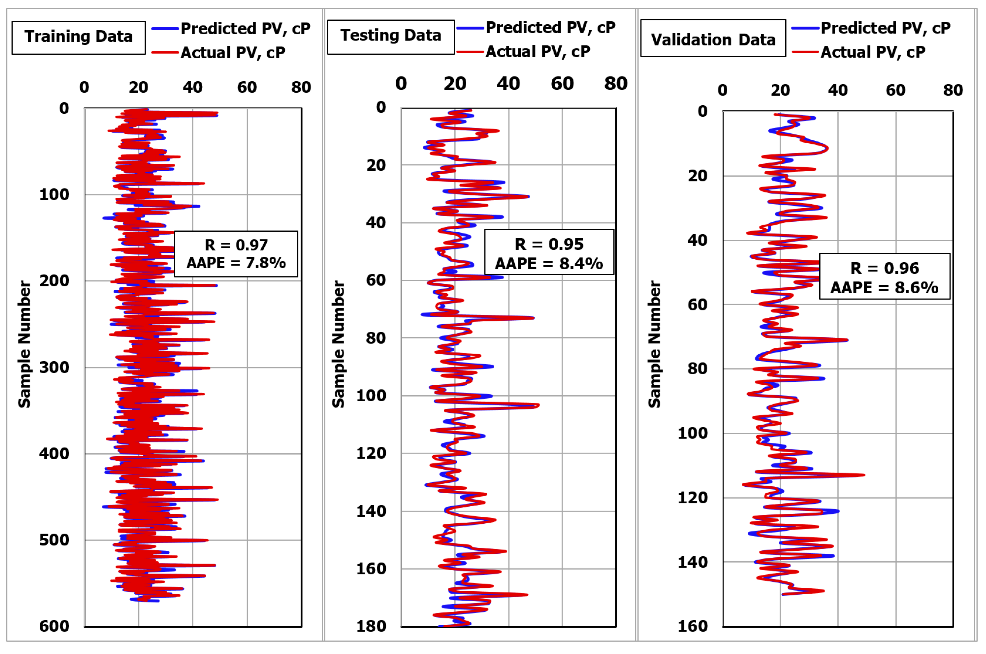
Figure 2 shows that the R was 0.97 and the AAPE was 7.8% between the actual and predicted PV for the training data. For testing the model, 180 data points were used. Figure 2 shows that the R was 0.95 and the AAPE was 8.4% between the actual and predicted PV for the testing data.

Figure 2. Prediction of plastic viscosity using the modified self-adaptive differential evolution-artificial neural network (MSaDE-ANN) technique.

The above results confirmed the high accuracy of using the MSaDE-ANN technique to predict the PV. For further validation, 150 unseen data points were used to evaluate the developed ANN-PV model. Figure 2 shows that the R was 0.96 and the AAPE was 8.6%, with an excellent match between the actual and predicted PV values for the validation points.

The same procedure was used to estimate the YP values using MD, FT, and SP. Training data (570 data points) were used to build the ANN-YP model. The optimization process after applying the MSaDE technique showed that the optimized number of neurons was 29, the optimum training function was Bayesian regularization backpropagation (trainbr), and the best transferring function was Elliot symmetric sigmoid (elliotsig).

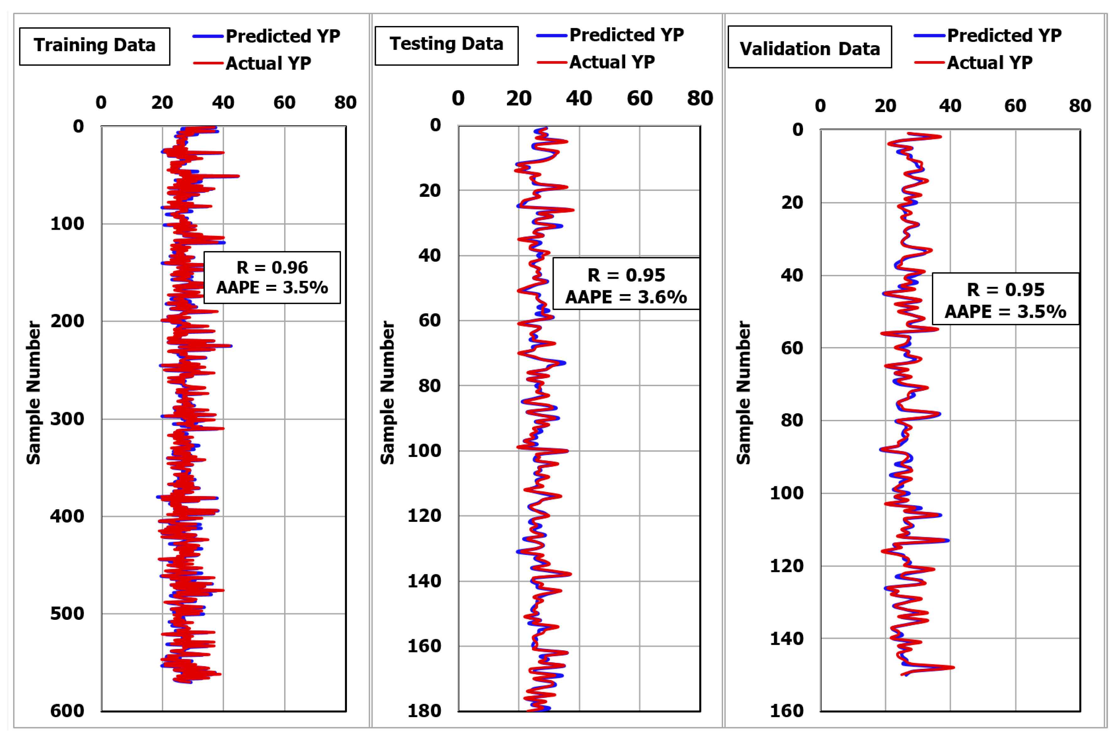
Figure 3 shows that the R was 0.96 and the AAPE was 3.5% when using the MSaDE-ANN model to predict the YP values for the training data set. To test the developed model for YP, another set of data (180 unseen data points) was used. Figure 3 shows that for the unseen data, the R was 0.95 and the AAPE was 3.6. These results confirmed the high accuracy of the MSaDE-ANN model for predicting the YP from the MD, FT, and SP.

Figure 3. Prediction of yield point using the MSaDE-ANN technique.

The flow behavior index (n) was used to describe the degree of fluid deviation from the standard Newtonian behavior. In other words, n was used to represent the degree of non-Newtonian behavior. For drilling fluids that act according to the pseudoplastic fluids behavior, the standard value of n is between zero and 1 [39], where the value is 1 for Newtonian fluids behavior and less than 1 for dilatant fluids. n also can be used as a representation of the shear-thinning properties of the drilling fluids. A fluid with a low value of n is good for hole cleaning purposes.

The flow behavior index (n) can be calculated through Equation (7) based on the values of PV and YP [40].

$$\mathrm{n}=3.32\ast \log \left(\frac{2\mathrm{PV}+\mathrm{YP}}{\mathrm{PV}+\mathrm{YP}}\right)$$

(7)

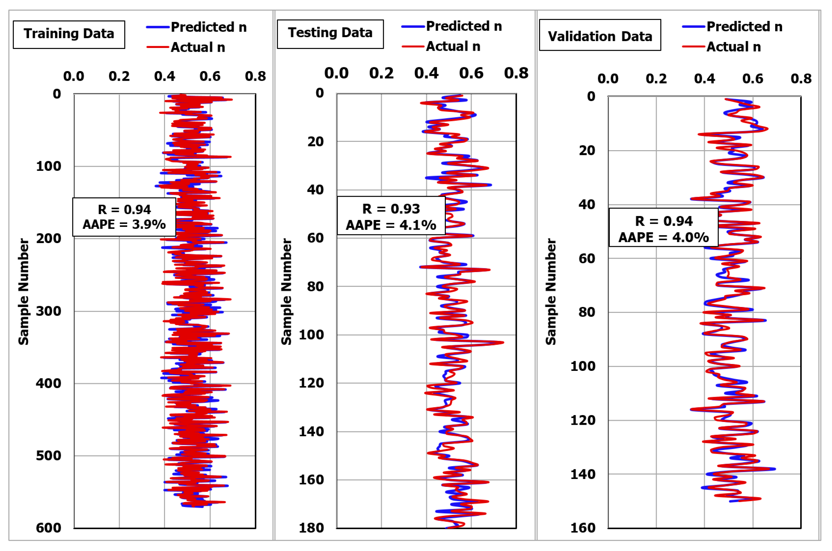
The MSaDE technique was applied to optimize the variable parameters of the ANN model for n. The optimization process yielded that the optimized number of neurons was 29, the optimum training function was Bayesian regularization backpropagation (trainbr), and the best transferring function was Elliot symmetric sigmoid (elliotsig).

Figure 4 shows that the MSaDE-ANN predicted n with high accuracy, where the R was 0.94 and the AAPE was 3.96% for the training dataset (570 data points). The same results were obtained when applying the ANN-n model for the unseen data set (180 data points). The R was 0.93 and the AAPE was 4.1% between the actual and predicted values of n, as seen in Figure 4.

Figure 4. Prediction of the flow behavior index using the MSaDE-ANN technique.

A new set of data was used to validate the developed ANN-n model (150 data points). Figure 4 shows the high accuracy of the developed model to calculate n values based on MD, FT, and SP. The R was 0.94 and the AAPE was 4.0% between the calculated and actual values of n.

The flow consistency index (K) can be calculated from the PV and YP values using Equation (8) [39].

$$\mathrm{K}=\frac{2\mathrm{PV}+\mathrm{YP}}{{1022}^{3.22\log \left(\frac{2\mathrm{PV}+\mathrm{YP}}{\mathrm{PV}+\mathrm{YP}}\right)}}$$

(8)

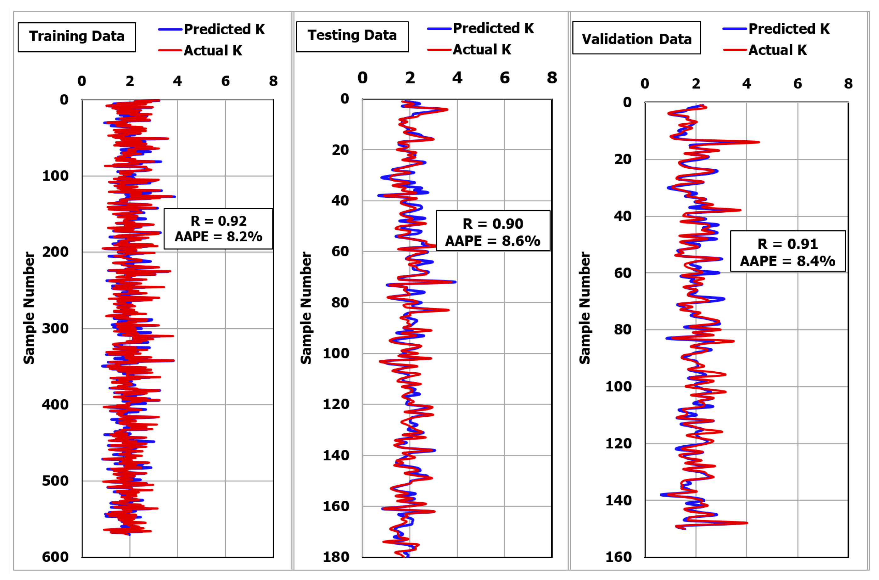
The optimization technique (MSaDE) was applied for the training dataset (570 data points) to determine the best combination of ANN variables to predict the K values based on MD, FT, and SP. The optimization process showed that the optimum number of neurons was 30, the optimum training function was Bayesian regularization backpropagation (trainbr), and the best transferring function was Elliot symmetric sigmoid (elliotsig).

Figure 5 shows that the R was 0.92 and the AAPE was 8.0% when plotting the actual and predicted values of K for the training dataset. For testing the developed ANN-K model, 150 unseen data points were used. Figure 5 shows that the R was 0.90 and the AAPE was 8.6% for the testing data.

Figure 5. Prediction of the consistency index using the MSaDE-ANN technique.

For further validation for the developed model for K, a new set of data was used (150 data points). Figure 5 shows that the R was 0.91 and the AAPE was 8.4% when plotting the calculated and actual values of K.

3.2. Development of Empirical Correlations

Plastic viscosity can be estimated using Equation (9) in normalized form using the weights and biases of the optimized PV-ANN model.

$${\mathrm{PV}}_{\mathrm{n}}={\displaystyle \sum }_{\mathrm{i}=1}^{ \mathrm{N}}{\mathrm{w}}_{2_{\mathrm{i}}}\frac{{\mathrm{w}}_{1_1}{\mathrm{MD}}_{\mathrm{n}}+{\mathrm{w}}_{1_2}{\mathrm{FT}}_{\mathrm{n}}+{\mathrm{w}}_{1_3}{\mathrm{SP}}_{\mathrm{n}}+{\mathrm{b}}_{1_{\mathrm{i}}}}{1+\left|{\mathrm{w}}_{1_1}{\mathrm{MD}}_{\mathrm{n}}+{\mathrm{w}}_{1_2}{\mathrm{FT}}_{\mathrm{n}}+{\mathrm{w}}_{1_3}{\mathrm{SP}}_{\mathrm{n}}+{\mathrm{b}}_{1_{\mathrm{i}}}\right|}+{\mathrm{b}}_2$$

(9)

where PV_n is the PV in the normalized form; N is the optimized number of neurons (30 neurons); w₁ and w₂ are the weights between the input layer and hidden layer and the weights between the hidden layer and the output layer, respectively (see Table 2); b₁ is the biases between the input layer and the hidden layer; b₂ = 0.073, which is the bias associated with hidden layer and output layer; and MD_n, FT_n, and SP_n are the normalized value of the MD, FT, and SP, respectively.

Table 2. Weight and biases for the MSaDE- ANN-PV (plastic viscosity) model.

i	w1,1	w1,2	w1,3	b1,i	w2,i
1	−0.583	1.507	−0.860	0.903	0.908
2	−3.501	−0.904	2.668	0.687	−3.538
3	1.808	−0.951	−1.900	−0.919	−1.791
4	−1.425	−0.233	0.978	0.831	1.730
5	0.694	−0.185	−2.284	−1.747	2.862
6	−0.437	−0.051	−2.132	0.938	2.268
7	−1.859	−0.960	−0.078	1.793	2.691
8	−1.938	0.218	−0.768	1.179	−1.546
9	−0.292	−0.861	1.351	0.265	2.066
10	−1.499	−1.501	−0.483	0.853	−2.594
11	2.684	−1.286	0.365	−0.872	2.682
12	−2.306	−1.507	0.739	0.798	2.175
13	−3.429	0.825	−0.812	0.612	2.935
14	−3.670	−0.562	2.914	0.212	3.500
15	−0.212	2.242	0.215	0.898	0.636
16	−3.783	0.359	−0.924	0.322	−2.874
17	1.841	0.508	−2.393	0.406	2.054
18	0.070	0.416	1.032	0.120	−1.277
19	−1.983	−1.337	−0.348	−1.039	−1.360
20	2.361	0.706	−1.352	0.682	−1.953
21	−0.433	1.532	−1.024	−0.416	0.591
22	3.936	−0.190	−0.664	1.675	2.266
23	−2.621	−0.446	1.632	−1.496	2.190
24	−3.587	−0.179	0.248	−1.957	3.859
25	0.391	2.102	−0.766	−0.486	0.718
26	−1.657	0.513	−1.322	2.493	−2.294
27	3.939	0.095	−0.526	2.303	3.056
28	2.624	−0.271	1.179	3.204	2.736
29	−1.101	0.296	−1.454	−1.872	2.617
30	−0.090	0.159	1.012	0.695	0.595

The de-normalized value of the PV can be obtained using Equation (10).

$$\mathrm{PV}=22.727\ast {\mathrm{PV}}_{\mathrm{n}}+28.727$$

(10)

Using the weights and biases of the optimized MSaDE-ANN model for YP, Equation (9) can be used to calculate the normalized value of YP by changing the ${\mathrm{PV}}_{\mathrm{n}}$ by ${\mathrm{YP}}_{\mathrm{n}}$. Equation (11) can be used to determine the actual value of YP. Table 3 list the values of w₁, w₂, i, and b₁. The value of b₂ was 1.309.

$$\mathrm{YP}=16.393\ast {\mathrm{YP}}_{\mathrm{n}}+28.393$$

(11)

Table 3. Weight and biases for the MSaDE-ANN-YP model.

i	w1,1	w1,2	w1,3	b1,i	w2,i
1	−1.221	1.308	2.159	1.233	1.591
2	−0.037	2.097	−0.212	−1.118	1.439
3	0.718	0.232	2.575	−1.190	−2.301
4	4.058	0.842	−0.047	−3.523	−2.752
5	1.106	2.035	1.657	−1.937	−1.485
6	−1.831	1.350	−0.601	0.126	−2.434
7	−0.374	−1.661	0.175	0.694	2.705
8	−0.911	1.444	1.932	0.630	1.460
9	3.782	−2.940	1.792	−0.087	−1.533
10	−2.465	−0.160	2.281	0.814	−2.687
11	−3.233	−0.544	−0.973	1.313	−3.472
12	4.663	0.189	−0.004	−1.128	−3.994
13	−3.581	0.020	−2.615	1.008	−3.412
14	−0.552	−0.904	1.216	−0.231	−0.450
15	0.232	−1.919	−2.035	0.649	−1.958
16	−1.575	−0.279	−2.414	0.708	2.612
17	−1.180	1.007	0.957	−0.032	−1.186
18	3.017	0.111	−2.673	0.428	0.984
19	−1.576	−0.403	1.255	−0.136	2.349
20	0.594	−1.155	−2.862	0.690	1.720
21	1.168	0.259	−3.619	1.469	−2.071
22	1.279	1.252	1.368	1.121	1.375
23	3.282	0.251	3.735	4.043	−2.204
24	1.963	0.661	1.648	1.578	−1.968
25	2.453	−0.114	2.042	2.638	3.704
26	1.825	0.060	1.069	2.281	−3.608
27	−0.513	−1.540	−0.980	1.370	−3.686
28	1.815	0.280	0.012	−1.744	2.755
29	2.985	−0.438	0.644	3.077	1.977

The normalized flow behavior index can be calculated using Equation (9) by changing ${\mathrm{PV}}_{\mathrm{n}}$ by ${\mathrm{n}}_{\mathrm{n}}$ based on the optimized ANN-n model by extracting the weights and biases. To obtain the de-normalized value of n, Equation (12) can be used. Table 4 lists the values of w₁, w₂, b₁, and i. b₂ was 1.209.

$$\mathrm{n}=0.226\ast {\mathrm{n}}_{\mathrm{n}}+0.516$$

(12)

Table 4. Weight and biases for the MSaDE-ANN-n (artificial neural network-flow behavior index) model.

i	w1,1	w1,2	w1,3	b1,i	w2,i
1	−0.443	−0.156	0.758	−0.485	−0.994
2	1.141	2.210	−0.648	−2.048	−1.732
3	0.939	1.042	0.370	−1.657	1.965
4	−0.176	1.325	−0.765	0.989	−1.317
5	0.365	−0.246	−2.876	−2.609	3.213
6	0.373	1.195	1.975	2.595	3.107
7	−2.520	−0.795	0.373	1.659	−2.423
8	−1.340	0.991	2.523	1.324	−2.301
9	−0.961	0.901	2.914	−0.831	2.361
10	−2.506	−0.345	4.267	−0.129	−2.154
11	1.981	−0.971	−0.055	−1.641	−2.219
12	−1.794	0.269	−1.606	0.618	1.510
13	0.218	−2.321	−1.555	0.361	0.814
14	2.416	0.465	−2.349	−0.419	−2.432
15	−0.614	1.457	1.175	0.794	0.851
16	3.914	0.056	−0.523	1.832	−3.468
17	2.065	0.085	1.889	−0.278	1.808
18	0.401	0.534	−2.224	−0.083	−1.622
19	3.154	−0.414	−0.337	1.019	−2.465
20	−1.901	−1.296	−0.574	−1.033	−1.579
21	2.438	−0.437	−4.073	1.524	2.822
22	4.731	−0.405	−0.561	1.886	3.552
23	−0.986	0.434	−1.951	−2.056	3.097
24	−3.643	−0.243	−0.544	−2.627	−2.013
25	0.342	0.091	−0.593	0.421	0.846
26	1.679	−0.291	−0.439	1.433	−2.427
27	−1.483	−0.556	2.154	−0.003	1.369
28	−2.376	−0.493	0.507	−2.083	3.200
29	−2.915	0.143	−1.838	−3.799	−3.532

The flow consistency index (K) can be estimated as a function of MD, FT, and SP using Equation (9) in a normalized form which was developed using the weights and biases of the optimized ANN-K model. The normal values of K can be calculated using Equation (13). Table 5 lists the values of w₁, w₂, b₁, and i. b₂ was −0.148.

$$\mathrm{k}=2.16\ast {\mathrm{K}}_{\mathrm{n}}+2.90$$

(13)

Table 5. Weight and biases for the MSaDE-ANN-K (artificial neural network-flow consistency index) model.

i	w1,1	w1,2	w1,3	b1,i	w2,i
1	−0.543	0.439	2.175	1.330	2.624
2	−1.067	−1.016	1.717	0.141	−1.152
3	−0.288	−0.348	−1.421	1.359	2.115
4	−2.822	−0.325	−0.492	0.816	1.942
5	−0.065	1.376	−0.993	−1.101	1.357
6	−0.462	1.782	0.506	1.347	−1.852
7	−0.952	−1.445	−0.386	1.426	−1.660
8	−2.003	−0.135	3.601	−0.129	2.638
9	−0.583	−1.707	0.477	0.618	1.754
10	0.117	1.851	1.359	−0.358	1.278
11	0.486	−0.749	−2.045	0.623	2.230
12	1.568	0.610	−0.380	−0.357	1.534
13	−2.644	0.202	−1.245	0.768	−2.811
14	1.429	−1.114	−0.571	0.095	−1.969
15	1.465	−2.126	−0.567	−0.087	1.053
16	2.855	−0.573	−0.995	0.830	2.813
17	1.486	0.230	−2.934	0.298	2.534
18	−1.656	−0.036	−2.234	0.405	1.775
19	−2.152	−1.729	−1.419	−1.295	1.239
20	1.276	0.531	2.234	1.557	−1.516
21	−1.246	0.749	−0.784	−1.348	−2.167
22	−3.413	0.427	0.067	−1.320	2.202
23	2.306	0.410	0.193	1.080	3.402
24	−4.026	0.409	2.392	−1.307	3.331
25	1.399	0.202	−2.729	1.177	−2.509
26	−2.946	0.447	2.470	−1.180	2.865
27	−0.856	−1.843	0.506	−1.775	−1.709
28	−3.792	0.467	2.515	−1.314	−3.679
29	−1.587	−0.228	−2.388	−3.075	3.192
30	1.722	−0.022	−0.091	1.562	2.176

AV can be calculated using Equation (9) as a function of MD, FT, and SP, which was developed based on the optimized ANN-AV model by extracting the weights and biases. Equation (14) can be used to calculate the de-normalized values of AV. Table 6 lists the values of w₁, w₂, b₁, and i. b₂ was −0.248.

$$\mathrm{AV}=10.73\ast {\mathrm{AV}}_{\mathrm{n}}+27.23$$

(14)

Table 6. Weight and biases for the MSaDE-ANN-AV (apparent viscosity) model.

i	w1,1	w1,2	w1,3	b1,i	w2,i
1	0.374	−1.536	0.574	0.882	−1.163
2	−1.408	1.125	−1.291	2.137	−3.658
3	−0.850	0.114	1.787	1.031	−2.843
4	0.062	1.644	0.325	−0.692	1.350
5	1.712	0.026	1.101	−1.484	2.197
6	−0.414	0.927	−1.626	0.997	2.071
7	2.731	0.188	0.132	−1.953	−2.308
8	1.872	−1.064	−0.627	−0.908	−1.324
9	−0.021	1.993	−0.154	0.632	0.597
10	−3.044	0.148	−0.800	0.982	3.794
11	−1.352	0.428	−2.180	−2.010	−1.469
12	−1.044	−0.865	2.198	−0.549	−1.772
13	3.590	0.253	1.442	−0.968	2.094
14	2.952	0.264	−2.643	−0.011	−1.670
15	−3.100	1.961	−0.781	1.463	−2.407
16	−1.318	−0.515	2.887	−0.371	2.183
17	−1.602	−0.282	2.118	−0.310	−2.710
18	−2.679	−0.947	1.475	−0.746	1.870
19	−1.975	0.530	0.362	−0.818	−2.142
20	−2.174	−1.062	0.256	−0.855	−1.848
21	0.285	−1.041	−0.577	0.283	1.225
22	2.634	0.435	−1.599	1.482	−2.305
23	−2.845	−0.052	−0.060	−1.538	2.172
24	−2.066	0.203	−0.763	−2.269	−2.080
25	0.872	−1.133	−0.508	0.858	1.674
26	−1.022	1.391	0.304	1.738	1.591
27	2.455	0.309	−0.406	1.484	2.241
28	2.346	−0.231	0.980	2.353	−2.973
29	0.641	0.218	1.541	1.810	1.331

3.3. Comparison with Previous Models

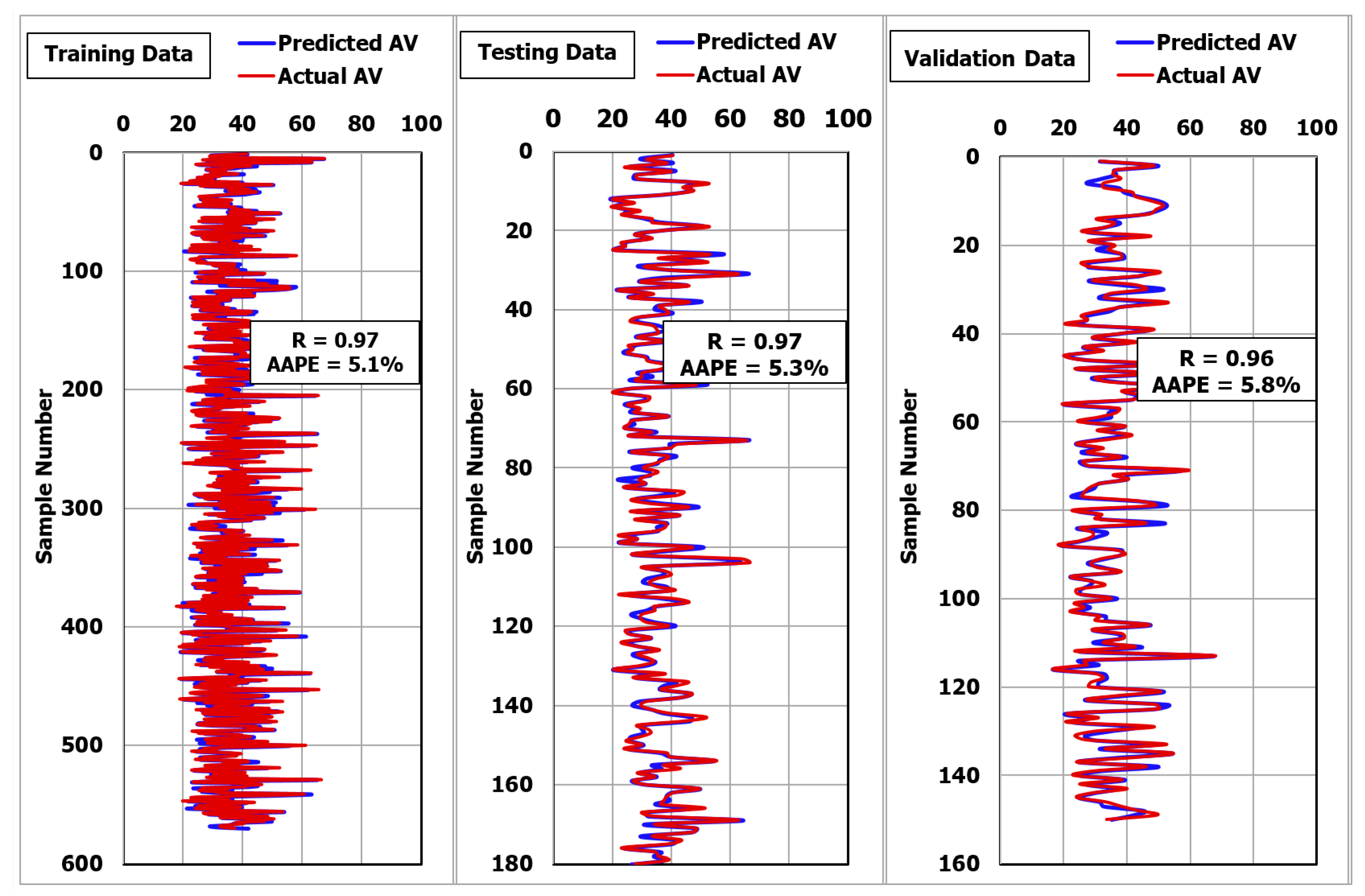
To compare the new MSaDE-ANN technique for the RHPs, the AV was predicted using the MSaDE-ANN, and the obtained results were compared with Pitt [41] and Almahdawi et al. [42]. The actual values of AV can be calculated based on PV and YP using Equation (15).

$$\mathrm{AV}=\frac{2\mathrm{PV}+\mathrm{YP}}{2}$$

(15)

Figure 6 shows the high accuracy of the developed ANN-AV model for the training dataset using the MSaDE technique. The R was 0.97 and the AAPE was 5.1% when plotting the predicted and actual AV values (570 data points). The same results were obtained for the testing data set, where the R was 0.97 and the AAPE was 5.3%, as can be seen in Figure 6.

Figure 6. Prediction of apparent viscosity using the MSaDE-ANN technique.

For the further validation of the AV developed ANN-AV model, a new data set was used (150 data points). Figure 6 shows that the R was 0.96 and the AAPE was 5.8% between the calculated and actual values of AV.

Pit [41] illustrated that the AV can be calculated as a function of MD and FT using Equation (16), while Almahdawi et al. [42] stated that AV can be determined using Equation (17).

$$\mathrm{AV}=\mathrm{MD}\ast \left(\mathrm{FT}-25\right)$$

(16)

$$\mathrm{AV}=\mathrm{MD}\ast \left(\mathrm{FT}-28\right)$$

(17)

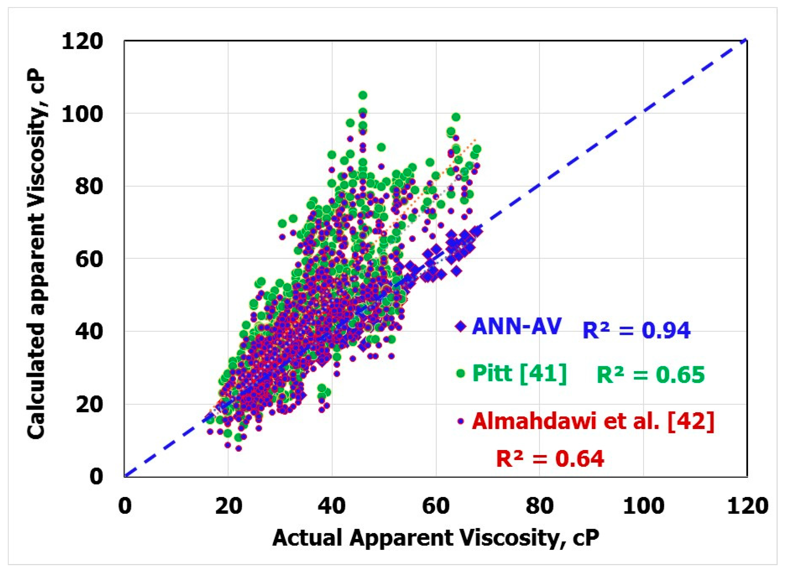
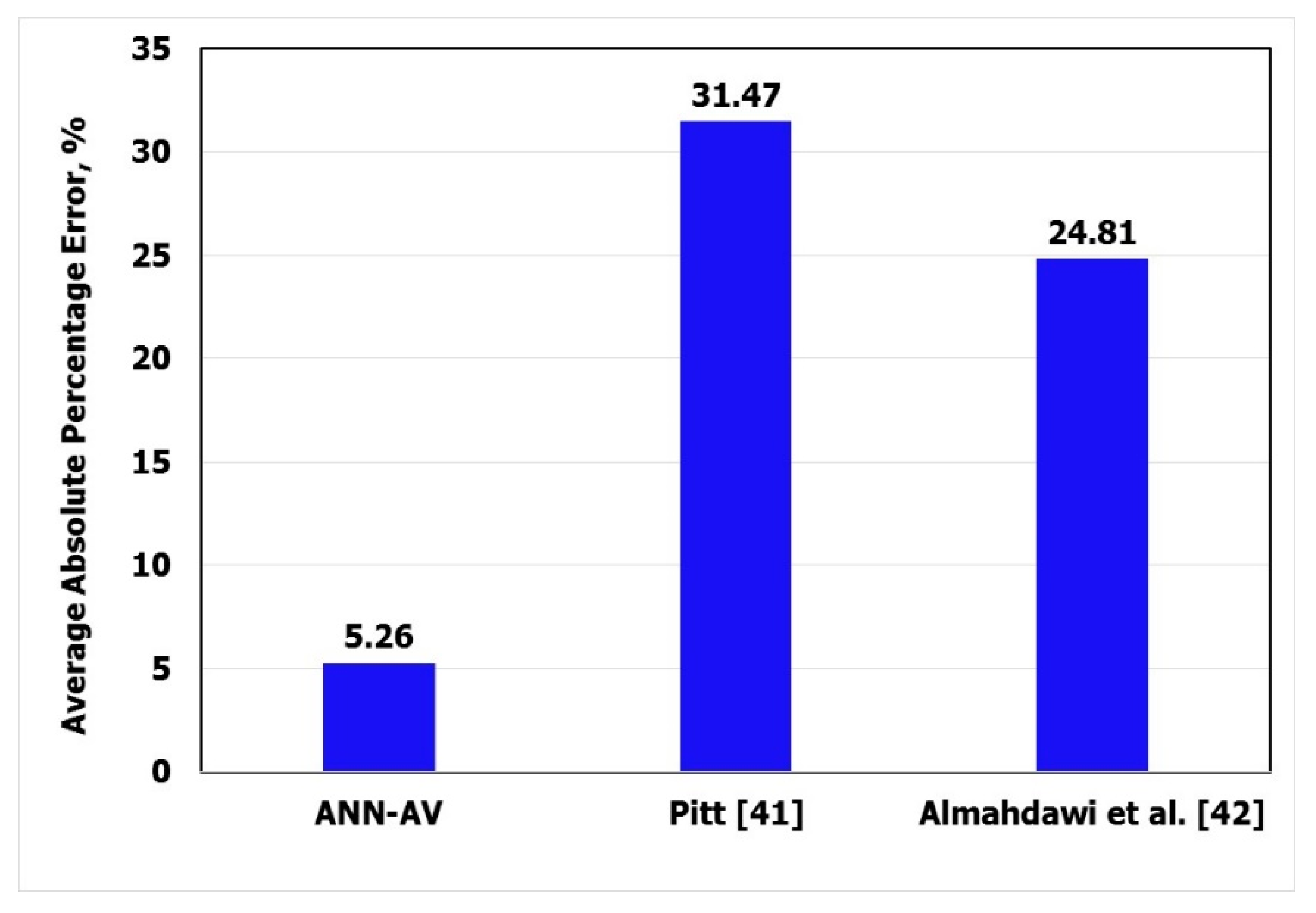
Applying Equations (16) and (17) using the available data sets (900 data points) showed that the ANN-AV model outperformed these models. Figure 7 shows that the coefficient of determination (R²) when plotting the calculated and actual valued of AV was 0.94 when the ANN-AV equation was used, 0.65 when Pitt’s equation was used, and 0.64 when Almahdawi’s equation was used. Figure 8 shows that the ANN-AV equation yielded the lowest AAPE (5.26%) as compared with the Pitt [41] equation (the AAPE was 31.47%) and the Almahdawi et al. [42] equation, where the AAPE was 24.81%.

Figure 7. Coefficient of determination for the apparent viscosity using different techniques.

Figure 8. Average absolute percentage error for calculating the apparent viscosity using different techniques.

3.4. Sensitivity Analysis

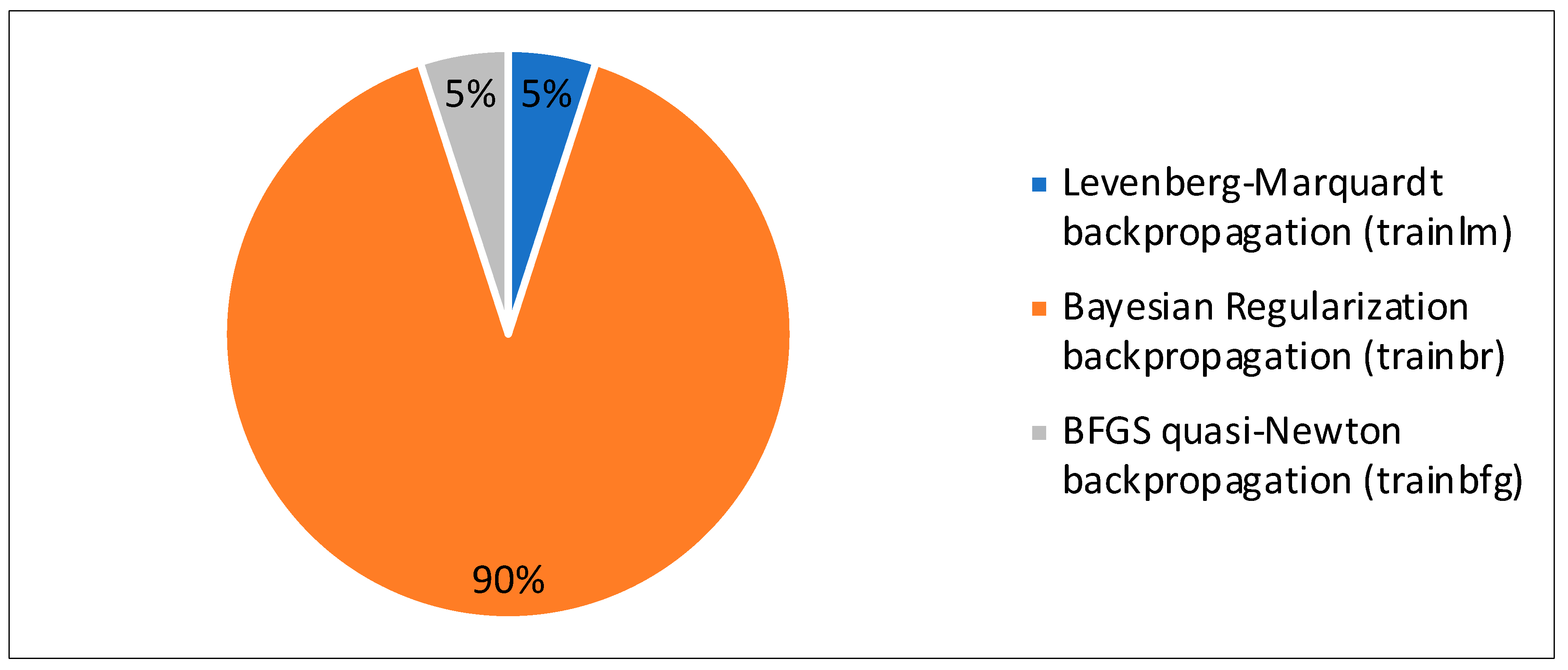
As mentioned earlier, the methodology of this study involved 20 independent optimization runs. Figure 9 shows that 18 out of the 20 optimization runs showed that the best training algorithm that achieved the best fit was the trainbr. The remaining two optimization runs were distributed equally between trainlm and trainbfg. This shows the consistency of this training function in achieving 90% of the best-fit performance compared to the other training algorithms. 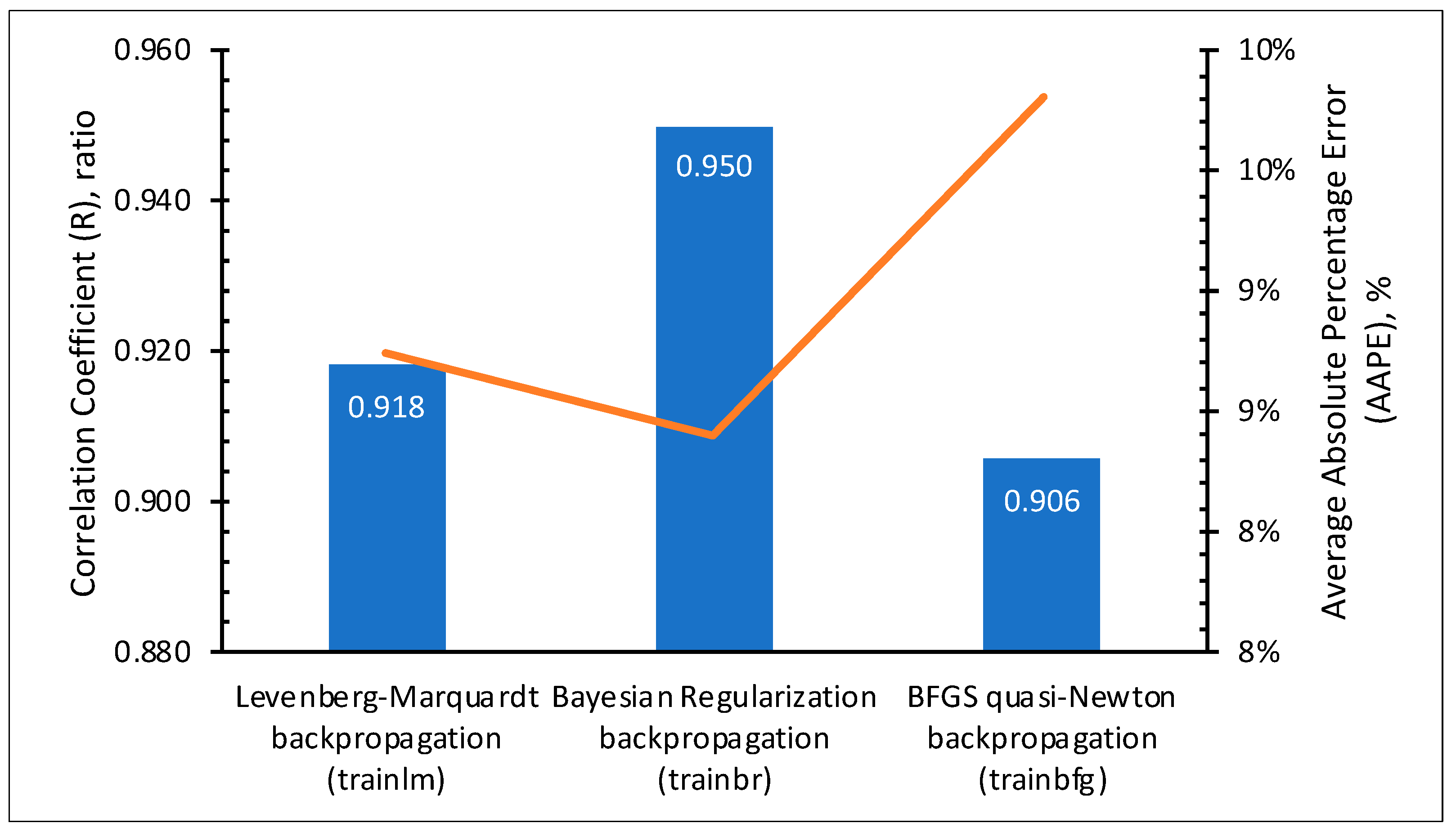Figure 10 shows the best results achieved by each of the three training algorithms. The figure demonstrates that trainbr achieved the highest R and the lowest AAPE. The outperformance of trainbr could be related to its backpropagation capability of minimizing a combination of the squared errors and weights to determine the optimum combination that produces an ANN that is able to generalize well by preventing the overfitting (preventing increasing values of weights).

Figure 9. The success percentage for each training algorithm.

Figure 10. Performance comparison of the training algorithms.

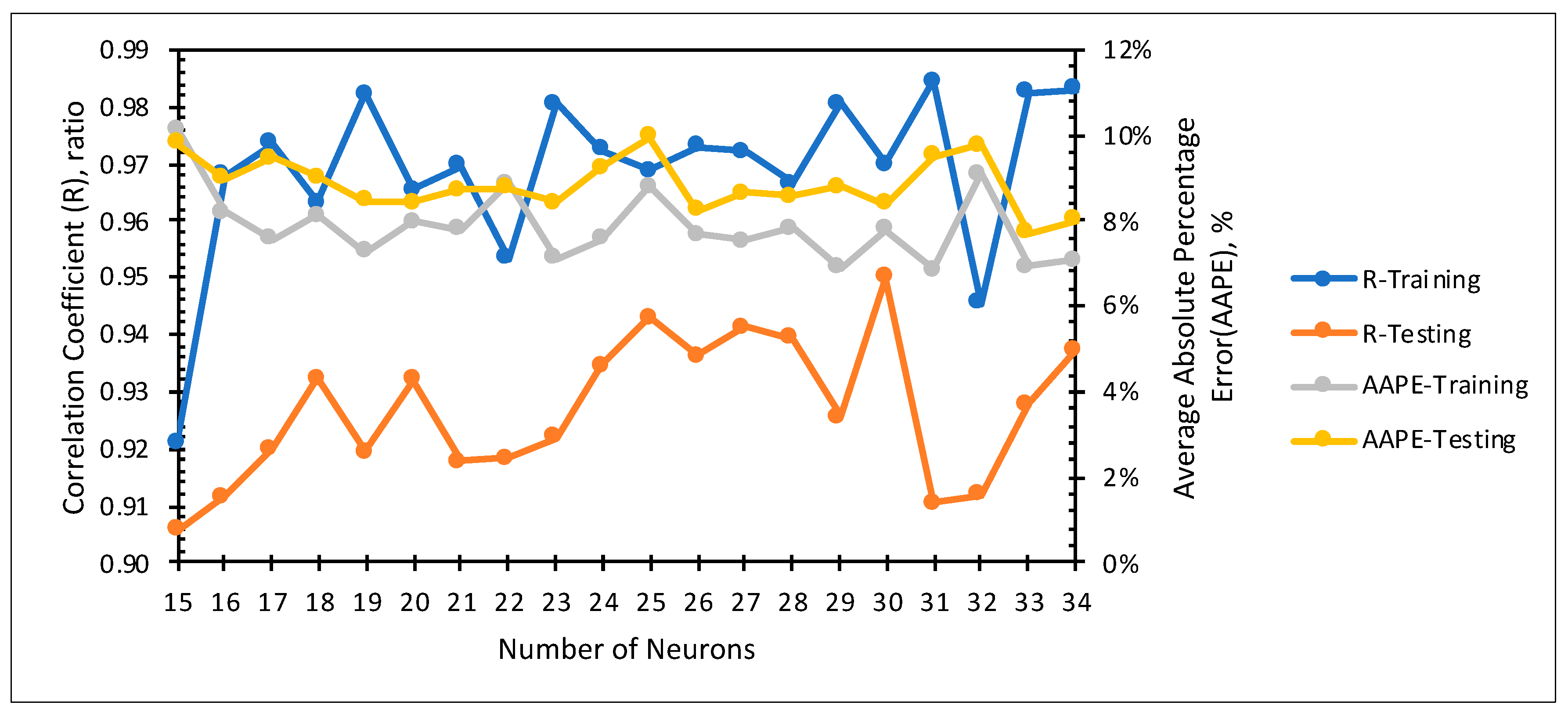
Figure 11 shows the sensitivity of the ANN performance to the number of neurons. The ANN performance indicators were the correlation coefficient (R) and the AAPE for the training and testing datasets. The figure demonstrates that, generally, increasing the number of neurons enhanced the ANN performance in terms of increasing the R of testing until reaching an optimum value of 30 neurons; then, the performance dropped. The reason for this behavior was the overfitting. Increasing the number of neurons to a very large value resulted in the ANN performing well on the training set but performing poorly on the testing set, which indicates overfitting. This is demonstrated by the figure, as it shows when the number of neurons increased more than 30, the R-value of training set generally increased, but the R-value of testing generally decreased. Therefore, the optimum number of neuron, in this case, was determined to be 30 neurons. Figure 12 shows the topography of the ANN with the optimized number of neurons.

Figure 11. Sensitivity analysis of the model performance to the number of neurons.

Figure 12. The topography of the artificial neural network.

4. Conclusions

The modified self-adaptive differential evolution technique was implemented to optimize the different variables of an ANN to determine the RHPs of NaCl-WBDIF using actual field measurements (900 data points) of MD, FT, and SP. Based on the obtained results, the following conclusions can be drawn:

• For all rheological properties, the optimization process showed that the best training function was Bayesian regularization backpropagation (trainbr) and the best transferring function was Elliot symmetric sigmoid (elliotsig).
• The optimum number of neurons was 30 for PV and K, while it was 29 for n, AV and YP.
• The developed ANN models predicted the RHPs with high accuracy. The R was more than 90%, and the AAPE was less than 8.6%.
• The five empirical equations for the RHPs were simple and accurate to be applied in a real-time without the need for ANN models or any special equipment.
• The AV empirical equations based on the optimized ANN model outperformed the previous AV models.

It is recommended to develop an automated Marsh funnel system that measures the mud density, Marsh funnel time, and solid percent using automated method, and the yielded results can be used as inputs for the developed ANN models, which can be used to estimate the rheological properties every 5–10 min. This will enable the driller to understand the changes in the drilling fluid properties as well as the changes in the rig hydraulics. This make decisions regarding the required action based on given information much faster.

References

- Zhang, X.; Jiang, G.; Xuan, Y.; Wang, L.; Huang, X. Associating Copolymer Acrylamide/Diallyldimethylammonium Chloride/Butyl Acrylate/2-Acrylamido-2-methylpropanesulfonic Acid as a Tackifier in Clay-Free and Water-Based Drilling Fluids. Energy Fuels 2017, 31, 4655–4662. [Google Scholar] [CrossRef]
- Zhang, L.-M.; Tan, Y.B.; Li, Z.M. Application of a new family of amphoteric cellulose-based graft copolymers as drilling-mud additives. Colloid Polym. Sci. 1999, 277, 1001–1004. [Google Scholar] [CrossRef]
- Luo, Z.; Pei, J.; Wang, L.; Yu, P.; Chen, Z. Influence of an ionic liquid on rheological and filtration properties of water-based drilling fluids at high temperatures. Appl. Clay Sci. 2017, 136, 96–102. [Google Scholar] [CrossRef]
- Bourgoyne, A.T.; Cheever, M.E.; Mulheim, K.K.; Young, F.S. Applied Drilling Engineering; SPE Textbook Series; Society of Petroleum Engineers: Richardson, TX, USA, 1986; Volume 2. [Google Scholar]
- Ahmad, H.M.; Kamal, M.S.; Al-Harthi, M.A. Rheological and Filtration Properties of Clay-Polymer Systems: Impact of Polymer Structure. Appl. Clay Sci. 2018, 160, 226–237. [Google Scholar] [CrossRef]
- Sadeghalvaad, M.; Sabbaghi, S. The effect of the TiO2/polyacrylamide nanocomposite on water-based drilling fluid properties. Powder Technol. 2015, 272, 113–119. [Google Scholar] [CrossRef]
- Lyons, W.C.; Plisga, J. Standard Handbook of Petroleum and Natural Gas Engineering, 2nd ed.; Gulf Publishing Company: Houston, TX, USA, 2005. [Google Scholar]
- Hossain, M.E.; Al-Majed, A.A. Fundamentals of Sustainable Drilling Engineering; Scrivener Publishing LLC: Salem, MA, USA, 2015. [Google Scholar]
- Adams, N.J. Drilling Engineering: A Complete Well Planning Approach; Penn Well Publishing Company: Tulsa, OK, USA, 1985. [Google Scholar]
- Kersten, G.V. Results and Use of Oil-Base Fluids in Drilling and Completing Wells. In Drilling and Production Practice; Paper API-46-061; American Petroleum Institute: New York, NY, USA, 1946. [Google Scholar]
- Luo, Y.; Bern, P.A.; Chambers, B.D. Simple Charts to Determine Hole Cleaning Requirements in Deviated Wells. In SPE/IADC Drilling; Paper SPE 27486; Society of Petroleum Engineers: Houston, TX, USA, 1994. [Google Scholar]
- Paiaman, A.M.; Al-Askari, M.K.G.; Salmani, B.; Al-Anazi, B.D.; Masihi, M. Effect of Drilling Fluid Properties on Rate of Penetration. NAFTA 2009, 60, 129–134. [Google Scholar]
- Okrajni, S.; Azar, J. The Effects of Mud Rheology on Annular hole Cleaning in Directional Wells. SPE Drill. Eng. 1986, 1, 297–308. [Google Scholar] [CrossRef]
- Robinson, L.; Morgan, M. Effect of hole cleaning on drilling rate performance. Paper AADE-05-DF-HO-41. In Proceedings of the AADE Drilling Fluid Conference, Houston, TX, USA, 6–7 April 2004. [Google Scholar]
- Marsh, H.N. Properties and Treatment of Rotary Mud. Trans. AIME 1931, 92, 234–251. [Google Scholar] [CrossRef]
- Balhoff, M.T.; Lake, L.W.; Bommer, P.M.; Lewis, R.E.; Weber, M.J.; Calderin, J.M. Rheological and yield stress measurements of non-Newtonian fluids using a Marsh Funnel. J. Pet. Sci. Eng. 2011, 77, 393–402. [Google Scholar] [CrossRef]
- McCulloch, W.S.; Pitts, W. A logical calculus of the ideas immanent in nervous activity. Bull. Math. Biophys. 1943, 5, 115–133. [Google Scholar] [CrossRef]
- Rosenblatt, F. The Perceptron, a Perceiving and Recognizing Automaton; Project Para Report No. 85-460-1; Cornell Aeronautical Laboratory (CAL): Buffalo, NY, USA, 1957. [Google Scholar]
- Bailey, D.; Thompson, D. How to Develop Neural Network. AI Expert 1990, 5, 38–47. [Google Scholar]
- Fausett, L. Fundamentals of Neural Networks, Architectures, Algorithms, and Applications; Prentice-Hall Inc.: Eaglewood Cliffs, NJ, USA, 1994. [Google Scholar]
- Ali, J.K. Neural Networks: A new Tool for the Petroleum Industry. Paper SPE-27561-MS. In Proceedings of the European Petroleum Computer Conference, Aberdeen, UK, 15–17 March 1994. [Google Scholar]
- Russell Stuart, J.; Norvig, P. Artificial Intelligence: A Modern Approach, 3rd ed.; Prentice Hall: Upper Saddle River, NJ, USA, 2009; ISBN 0-13-604259-7. [Google Scholar]
- Sargolzaei, J.; Saghatoleslami, N.; Mosavi, S.M.; Khoshnoodi, M. Comparative Study of Artificial Neural Networks (ANN) and statistical methods for predicting the performance of Ultrafiltration Process in the Milk Industry. Iranian. J. Chem. Eng. 2006, 25, 67–76. [Google Scholar]
- Lippmann, R. An introduction to computing with neural nets. IEEE ASSP Mag. 1987, 4, 4–22. [Google Scholar] [CrossRef]
- Mao, J.; Mohiuddin, K.; Jain, A. Artificial neural networks: A tutorial. Computer 1996, 29, 31–44. [Google Scholar]
- Demuth, H.B.; Beale, M.H.; Hagan, M.T. Neural Network Toolbox 6, User’s Guide; MathWorks, Inc.: Natick, MA, USA, 2009. [Google Scholar]
- AlAjmi, M.D.; Alarifi, S.A.; Mahsoon, A.H. Improving Multiphase Choke Performance Prediction and Well Production Test Validation Using Artificial Intelligence: A New Milestone. SPE-173394-MS. In Proceedings of the SPE Digital Energy Conference and Exhibition, Woodlands, TX, USA, 3–5 March 2015. [Google Scholar]
- Alarifi, S.A.; AlNuaim, S.; Abdulraheem, A. Productivity Index Prediction for Oil Horizontal Wells Using Different Artificial Intelligence Techniques. SPE-172729-MS. In Proceedings of the SPE Middle East Oil & Gas Show and Conference, Manama, Bahrain, 8–11 March 2015. [Google Scholar]
- Chen, F.; Duan, Y.; Zhang, J.; Wang, K.; Wang, W. Application of neural network and fuzzy mathematic theory in evaluating the adaptability of inflow control device in horizontal well. J. Pet. Sci. Eng. 2015, 134, 131–142. [Google Scholar]
- Van, S.L.; Chon, B.H. Effective Prediction and Management of a CO2 Flooding Process for Enhancing Oil Recovery using Artificial Neural Networks. ASME J. Energy Resour. Technol. 2017, 140, 032906. [Google Scholar] [CrossRef]
- Van, S.L.; Chon, B.H. Evaluating the critical performances of a CO2–Enhanced oil recovery process using artificial neural network models. J. Pet. Sci. Eng. 2017, 157, 207–222. [Google Scholar] [CrossRef]
- Qin, A.K.; Huang, V.L.; Suganthan, P.N. Differential Evolution Algorithm with Strategy Adaptation for Global Numerical Optimization. IEEE Trans. Evol. Comput. 2009, 13, 398–417. [Google Scholar] [CrossRef]
- Storn, R.; Price, K. Differential Evolution—A Simple and Efficient Heuristic for global Optimization over Continuous Spaces. J. Glob. Optim. 1997, 11, 341–359. [Google Scholar] [CrossRef]
- Moussa, T.M.; Awotunde, A.A. Self-adaptive differential evolution with a novel adaptation technique and its application to optimize ES-SAGD recovery process. Comput. Chem. Eng. 2018, 118, 64–76. [Google Scholar] [CrossRef]
- Al-Khdheeawi, E.A.; Mahdi, D.S. Apparent Viscosity Prediction of Water-Based Muds Using Empirical Correlation and an Artificial Neural Network. Energies 2019, 12, 3067. [Google Scholar] [CrossRef]
- Gowida, A.; Elkatatny, S.; Ramadan, E.; Abdulraheem, A. Data-Driven Framework to Predict the Rheological Properties of CaCl2 Brine-Based Drill-in Fluid Using Artificial Neural Network. Energies 2019, 12, 1880. [Google Scholar] [CrossRef]
- Zhang, Y.; Pan, C.; Chen, X.; Wang, F. Abnormal breast identification by nine-layer convolutional neural network. J. Comput. Sci. 2018, 27, 57–68. [Google Scholar] [CrossRef]
- Wang, S.; Rao, R.V.; Chen, P.; Liu, A.; Wei, L. Abnormal Breast Detection in Mammogram Images by Feed-forward Neural Network Trained by Jaya Algorithm. Fundam. Inform. 2017, 151, 191–211. [Google Scholar] [CrossRef]
- Metzner, A.B. Non-Newtonian technology: Fluid mechanics and transfers. Adv. Chem. Eng. 1956, 1, 77–153. [Google Scholar]
- Savins, J.G.; Roper, W.F. A Direct Indicating Viscometer for Drilling Fluids. Paper API-54-007. In Proceedings of the Drilling and Production Practice, New York, NY, USA, 1 January 1954. [Google Scholar]
- Pitt, M.J. The Marsh Funnel and Drilling Fluid Viscosity: A New Equation for Field Use. SPE Drill. Complet. 2000, 15, 3–6. [Google Scholar] [CrossRef]
- Almahdawi, F.H.; Al-Yaseri, A.Z.; Jasim, N. Apparent Viscosity Direct from Marsh Funnel Test. Iraqi J. Chem. Pet. Eng. 2014, 15, 51–57. [Google Scholar]
© 2019 by the author. Licensee MDPI, Basel, Switzerland. This article is an open access article distributed under the terms and conditions of the Creative Commons Attribution (CC BY) license (http://creativecommons.org/licenses/by/4.0/).