Abstract
This paper proposes a collaborative optimization strategy of regenerative braking in heavy-duty electric logistics vehicles under complex driving conditions to improve energy recovery efficiency. Based on the actual operational data of 18-ton electric trucks in the southwestern region of China, three driving scenarios for heavy commercial vehicles are determined via the K-Means clustering algorithm. Key features are extracted using Recursive Feature Elimination and employed to train a Learning Vector Quantization neural network for precise real-time condition recognition. The identified driving condition parameters, including vehicle speed, remaining battery power, and braking force, collectively regulate the intensity of regenerative braking. Simulation results under double-WTVC (World Transient Vehicle Cycle) conditions indicate that the proposed strategy can effectively adapt regenerative braking behavior to diverse road conditions. In comparison with conventional control methods, this approach enhances battery energy recovery efficiency by 5.8% while preventing control discontinuities.
1. Introduction
China dominates the global express delivery market, handling a parcel volume that exceeds the combined total of the United States, Japan, and Europe, accounting for over half of the world’s total [1,2]. This scale renders improving the efficiency, safety, and environmental performance of the logistics fleet critically imperative. Vehicle electrification is a key pathway, with RBSs offering significant potential to enhance energy efficiency by recovering kinetic energy during deceleration. Studies indicate that recovery efficiency can reach up to 79% under low-intensity braking [3,4,5].
Regenerative braking is a well-established technology for hybrid and electric vehicles, aimed at extending driving range and reducing brake wear emissions [6,7,8]. Consequently, optimizing RBS control strategies is a major research focus in vehicle electrification [9,10,11,12]. Extensive research has produced advanced solutions, particularly for passenger cars and hybrid vehicles. This includes strategies focused on optimal braking force distribution and coordination between regenerative and hydraulic systems [13,14,15], energy management for complex hybrid powertrains integrating fuel cells or supercapacitors [16,17], and adaptive controls that consider driving style or environmental conditions [13,18].
However, the effectiveness of these strategies diminishes when applied to heavy-duty electric logistics vehicles. The core issue is a mismatch between system design and operational reality. Most existing RBSs are developed based on passenger vehicle paradigms, yet logistics trucks face fundamentally different conditions: significant load fluctuations between empty and fully laden states, and operational profiles characterized not by frequent urban stop–start cycles, but by long-haul, sustained-speed travel on diverse road types (e.g., highways, hilly roads, national roads) [19,20,21]. This mismatch leads to significant performance fluctuations in real-world operation. Fixed-threshold strategies often trigger inappropriate mechanical braking intervention during load transitions or fail to adapt to varying road conditions, resulting in suboptimal energy recovery.
This gap highlights a distinct and significant opportunity. Unlike city buses with limited kinetic energy per stop, heavy-duty trucks on long routes possess substantial kinetic energy during high-speed deceleration, offering greater recovery potential. Therefore, developing adaptive RBS strategies specifically tailored to the high-speed, mixed-condition driving cycles and unique dynamics of heavy-duty electric trucks is crucial to maximize their range, operational economy, and viability in the logistics market.
To address this need, this paper proposes a novel strategy for an 18-ton pure electric logistics truck that integrates data-driven driving condition recognition with adaptive fuzzy control. The strategy dynamically regulates regenerative braking intensity based on real-time identification of road type (plain highway, hilly expressway, national highway), vehicle speed, battery state of charge, and braking demand—all while strictly guaranteeing braking safety. The vehicle parameters discussed are shown in Table 1.

Table 1.
Vehicle parameters.
The principal contributions of this study are as follows: (1) the dynamic adjustment of braking performance in accordance with driving environments; (2) the maximization of energy recovery through advanced driving condition identification and optimization algorithms.
Moreover, to verify the efficacy of the proposed strategy, a vehicle model was established in MATLAB/Simulink (2020a). Comparative simulations between the conventional strategy and the proposed approach revealed a significant improvement in SOC, highlighting the potential of this strategy to extend the driving range and curtail energy consumption in commercial vehicles.
The vehicle investigated in this study is an 18-ton heavy-duty electric logistics truck produced by Dongfeng Liuzhou Motor Co., Ltd., Liuzhou, China. It features a rear-wheel-drive pure electric powertrain, where the traction motor is capable of regenerative braking on the rear axle, while the front axle is equipped with a conventional pneumatic friction braking system. This configuration presents a typical challenge for optimizing regenerative braking energy recovery while ensuring braking stability and safety regulations.
The following sections of this paper are structured as follows. Section 2 develops a machine-learning model for driving condition recognition. Section 3 proposes a regenerative braking strategy that integrates both braking safety regulations and real-time driving conditions, and details the vehicle model developed for validation. Section 4 presents a comparative simulation analysis between the proposed strategy and conventional methods. Finally, Section 5 summarizes the research and offers concluding remarks.
2. Driving Condition Identification
2.1. Clustering Analysis of Driving Data
The real-world driving data used in this study were collected from 18-ton pure electric logistics trucks operated by Dongfeng Liuzhou Motor Co., Ltd. in Southwest China. The dataset comprises 555 processed trip segments, covering diverse road types including national highways, hilly expressways, and plain highways. Key temporal features such as vehicle speed, acceleration, and deceleration were recorded. To support open research in this field, the anonymized dataset has been made publicly available on GitHub [22].
Clustering analysis, an unsupervised learning algorithm, can group data with similar characteristics into the same category without labeled input. Among various clustering algorithms, K-means clustering is one of the most extensively utilized algorithms. It is regarded as a well-established method owing to its simplicity, rapid convergence, and low memory consumption [23]. K-Means clustering analysis was conducted on the driving speed data of fully loaded 18-ton heavy commercial vehicles in Southwest China. It was determined that the optimal number of clusters is three. The clustering performance and representative trip segments of each of the three resulting driving condition categories are presented in Figure 1 and Figure 2, respectively.
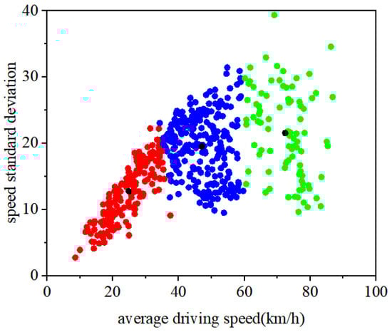
Figure 1.
Clustering Results of Speed Standard Deviation and Average Driving Speed.
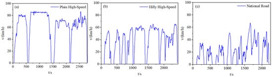
Figure 2.
Three types of clustering conditions: (a) Driving Cycle under Plain High-Speed Conditions. (b) Driving Cycle under Hilly High-Speed Conditions. (c) Driving Cycle under National Road Conditions.
In the clustering results diagram, red points indicate trip segments classified as national road conditions, blue points denote segments under hilly highway conditions, and green points represent segments categorized as plain highway conditions. The black points mark the cluster centers for the three categories. Observations show that the clusters are clearly separated, with distinctly distinguishable centers, indicating effective clustering performance.
As illustrated in Figure 2, the driving cycles can be broadly categorized into three typical patterns based on road topology and speed characteristics. Under plain high-speed conditions, trip segments tend to exhibit relatively long durations with smooth and stable driving behaviors. Vehicle speeds remain consistently high, with the maximum speed maintained at approximately 80 km/h, reflecting typical expressway or highway operation. In contrast, hilly high-speed conditions are associated with shorter segment durations and more fluctuating driving patterns. The maximum speed in these segments generally falls between 60 km/h and 70 km/h, indicating the influence of variable terrain and more frequent mode transitions. National road conditions, on the other hand, are characterized by the shortest driving durations and the most irregular driving behavior. While the maximum speed is similar to that observed in hilly scenarios, the average speed is significantly lower, and the frequency of acceleration and deceleration events is notably higher, suggesting a more complex traffic environment with frequent stops, variable speed limits, and mixed road users.
2.2. Feature Screening
Feature selection is a pivotal step in the development of high-performance driving condition recognition models, as it significantly enhances model performance and interpretability. The model proposed by Montazeri-Gh et al., which solely relies on vehicle speed parameters [24], has significant limitations in real-world complex driving scenarios. Research by Luo Yutao’s team [25] demonstrated that using only two parameters, average speed and travel distance, can only achieve fuzzy recognition. In contrast, incorporating ten features such as travel time for clustering analysis can yield more precise and quantifiable condition classification. These studies highlight a crucial insight: the number of selected features must strike a balance between representational capacity and computational efficiency. Insufficient parameters may fail to fully capture driving patterns, whereas an excessive number of parameters can introduce the curse of dimensionality, complicating the analysis.
Ericsson E’s research initially employed 62 characteristic parameters to characterize the driving patterns of trip segments, with the aim of laying a foundational framework for driving cycle construction, condition recognition model development, and investigations into vehicle pollutant emissions and energy management strategies [26]. However, this extensive feature set exhibited notable limitations: certain parameters were found to be irrelevant to the characterization of driving conditions; numerous features exhibited strong correlations with one another or could be derived via mathematical transformations, leading to data redundancy; furthermore, the effects of specific parameters were counteracted by others under real-world driving conditions, thereby diminishing their contribution to model performance. Given these issues, rigorous feature selection is deemed essential to enhance model interpretability, reduce computational complexity, and improve predictive accuracy. As a result, 22 parameters closely associated with vehicle driving conditions were selected from the original 62. These 22 characteristics are listed in the following order: average driving speed, mean acceleration, average deceleration, proportion of constant-speed driving, speed standard deviation, standard deviation of acceleration, standard deviation of deceleration, proportion of 0–10 km/h, proportion of 10–20 km/h, proportion of 20–30 km/h, proportion of 30–40 km/h, proportion of 40–50 km/h, proportion of 50–60 km/h, proportion of 60–70 km/h, proportion of 70–80 km/h, proportion of 80–90 km/h, proportion of 90–100 km/h, average frequency value of a >2 per 100 m, average frequency value of a >10 per 100 m, average frequency value of a >2 per 100 s, average frequency value of a >10 per 100 s, and mean value of the square of acceleration. This preliminary screened set retains the core information of vehicle driving dynamics while avoiding obvious redundancy, serving as the candidate feature pool for subsequent refinement.
The core function of the Recursive Feature Elimination method is to select the optimal subset of features from a high-dimensional feature set in order to improve model performance, reduce computational costs, and enhance the interpretability of the results. The RFE method was adopted to iteratively train the model and remove the least important features. This method uses random forest as the base model, and the number of trees set is 100. Resulting in the selection of an optimal subset comprising nine driving condition feature parameters, selecting results are shown in Figure 3. These nine features are a subset of the aforementioned 22 candidate parameters, specifically including the following: average driving speed, proportion of constant-speed driving, proportion of 0–10 km/h, proportion of 20–30 km/h, proportion of 30–40 km/h, proportion of 50–60 km/h, proportion of 60–70 km/h, proportion of 70–80 km/h, and proportion of 80–90 km/h.
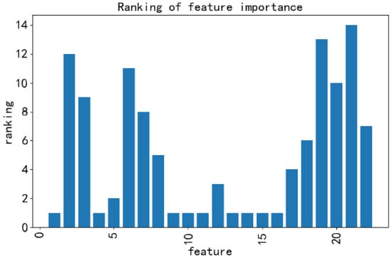
Figure 3.
The feature selection results obtained by the RFE method are sorted according to the order of the previous 22 features.
2.3. Driving Condition Identification Model
The LVQ neural network, introduced by Teuvo Kohonen, is a supervised classification model that operates using prototype vectors [27]. It represents a simplified form of competitive neural networks. For the task of real-time driving condition recognition in vehicle control systems, LVQ was selected over other common classifiers (e.g., SVM, Random Forest, MLP) due to its lower computational complexity and memory footprint, which are critical for feasible implementation on embedded hardware with limited resources, while maintaining high classification accuracy.
The values of the nine feature parameters obtained in Section 2.2 for each trip segment, along with their corresponding driving condition labels, were used as input to train an LVQ-based condition recognition model. Through this process, the model learns the general characteristics of segments belonging to each driving condition category based on these nine features—effectively training the weight vectors of the neurons in the competitive layer. After training, the model was tested on unseen trip segments to classify their driving conditions. The predicted categories were compared with the ground-truth labels to validate the recognition accuracy. The computational steps of the LVQ algorithm are as follows:
(1) Calculate the Euclidean distance between neurons in the competition layer and the input vector using the following formula:
where i is the index of competitive layer neurons, denotes the Euclidean distance between the i-th competitive layer neuron and the input feature vector, R represents the total number of feature parameters in the input vector, is the specific value of the j-th feature in the input vector, refers to the weight of the j-th feature corresponding to the i-th competitive layer neuron, and S denotes the total number of competitive layer neurons.
(2) The input vector corresponds to class Cx neuron a corresponds to class Ca, and neuron b corresponds to class Cb.
(3) If neurons a and b correspond to different classes, i.e., Ca ≠ Cb, and the distances from each neuron to the current input vector, denoted as da and db, satisfy the following condition:
where ρ represents the window width within which the input vector may fall close to the mid-plane between the two neurons, typically set to 2/3. Then, if Ca = Cx, neuron a will move its weight vector closer to the input vector, while neuron b will move its weight vector away from the input vector. The weight update formulas for the two neurons are as follows:
In Equation (3), ωanew and ωbnew represent the updated weight vectors of neurons a and b relative to the input vector; ωaold and ωbold denote the original weight vectors of neurons a and b relative to the input vector; α is the learning rate, with α > 0.
If Cb = Cx, neuron a will move its weight vector away from the input vector, while neuron b will move its weight vector closer to the input vector. The weight update formulas for the two neurons are as follows:
For the case where Ca ≠ Cx and Cb ≠ Cx, both neuron a and neuron b will cause their weight vectors to move away from the input vectors. The weight update formulas for the two neurons are as follows:
The purpose of this operation is to increase the distance between these two neurons, allowing one to move closer to the input vector. This process facilitates the retention of the optimal neuron, which ultimately activates the linear output layer neuron to complete the classification of the input vector.
If Equation (2) is not satisfied, or if neurons a and b belong to the same class, then the step of updating the weight vector will be carried out separately. In this case, if Ci = Cx, the weight vector is updated according to the following formula:
If Ci ≠ Cx, the weight vector is updated according to the following formula:
Before any model training, the complete set of 555 processed trip segments was randomly shuffled and split into a training set (80%) and an independent test set (20%). The test set was set aside and never used during model development, feature selection, or hyperparameter tuning. The proposed model architecture consists of nine input features, three output classes, five prototype vectors, and 15 competitive neurons, with an initial learning rate set to 0.01. During the training phase, a stepwise learning rate decay strategy was employed: after completing the first training epoch with the preset initial learning rate, the learning rate was reduced by a fixed increment of 0.0001 per subsequent epoch. This decay mechanism was maintained throughout the entire training process, which spanned 100 epochs in total. Experimental results on the test set demonstrated a recognition accuracy of 94.59%, while the recognition performance on the training set is illustrated in Figure 4. To further verify the model’s robustness, five-fold cross-validation was conducted, yielding consistent accuracy rates above 90%. These results collectively confirm the model’s strong generalization capability.

Figure 4.
The model prediction results of the test set.
3. Regenerative Braking Strategy Based on Recognized Driving Conditions
3.1. Braking Safety
Braking safety is the primary consideration during deceleration. The distribution strategy for braking forces between the front and rear axles is formulated in accordance with the European ECE braking regulations and China’s national standard Technical Requirements and Testing Methods for Commercial Vehicle and Trailer Braking Systems (GB 12676-2014) [28]. The utilization adhesion coefficients of the front and rear axles (denoted as φf and φr, respectively) must satisfy the following requirement:
Maintaining braking force within this safe distribution corridor not only ensures stability but also prevents abnormal braking conditions (e.g., premature lock-up or extreme force imbalance). Such abnormal conditions, which are precluded by the proposed strategy, are known to contribute to accelerated brake pad wear and induce additional stress on the chassis and suspension components [29].
The distribution of braking forces between the front and rear axles can be expressed using the braking force distribution coefficient β. Based on the conversion relationship between the braking force distribution coefficient and the adhesion coefficients of the front and rear axles, the braking force distribution coefficient β satisfies the following equation:
By integrating the above equations, the functional curve of the braking force distribution coefficient β under standard load conditions for heavy-duty commercial vehicles—derived within a safe range of braking intensity—is shown in Figure 5.
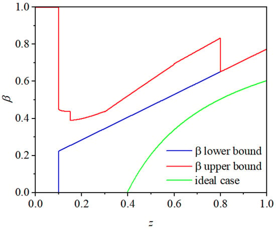
Figure 5.
Braking Force Distribution Coefficient Curves: Regulatory Requirements vs. Ideal Case.
As shown in Figure 5, the red curve represents the maximum allowable braking force distribution coefficient according to regulations, while the blue curve indicates the minimum required value. The green curve corresponds to the ideal braking force distribution coefficient for maximizing regenerative braking energy recovery. When the braking intensity z is less than 0.1, regulations do not explicitly specify the range for the braking force distribution coefficient β. In this study, the permissible range for β under full load is considered [0, 1]. However, when β = 0, it implies that the front axle contributes no braking force, relying solely on the rear axle—a condition that may be acceptable at low braking intensities but becomes increasingly unstable as z rises and should be avoided. For z ≥ 0.1, the value of β must fall within the region bounded by the ideal braking force distribution curve and the regulatory limits. The green curve illustrates an ideal scenario where braking is entirely provided by the electric motor, based on its maximum achievable braking torque. In this case, when z < 0.1, β is set to 0 to maximize regenerative energy recovery. When z ≤ 0.1, the electric motor supplies the total braking force until its torque limit is exceeded, at which point front-axle pneumatic braking is engaged without participation from the rear axle. This curve reflects the distribution of β that maximizes energy recovery under the described conditions. To optimize both energy recovery efficiency and braking safety, the actual control strategy references the blue curve for selecting β. This curve ensures operation within the regulatory region while allocating more braking force to the rear axle for regeneration, unlike the yellow curve, which violates the safety boundary.
3.2. Quantitative Analysis of Driving Condition Categories
Based on the braking safety constraints established in Section 3.1, the regenerative braking strategy needs to dynamically adjust the proportion of braking force distribution according to the driving conditions. However, the traditional strategy employs a discrete classification method for driving conditions (such as directly dividing conditions into three categories: high-speed, mountain roads, and national highways), which ignores the continuous transitional characteristics of ‘acceleration—constant speed—deceleration’ in actual driving, resulting in a step-like sudden change in the regenerative braking ratio, which not only affects the braking smoothness but also reduces the energy recovery efficiency. To solve this problem, this section proposes a continuous quantitative analysis method for driving conditions by constructing a quantitative function and a confidence function, converting discrete driving conditions into continuous adjustable parameters, achieving a smooth transition of braking force distribution, and precisely matching the energy recovery requirements under different driving conditions. The core idea of condition quantification is: by calculating the similarity between the current driving characteristics and various prototype vectors of different conditions (i.e., the Euclidean distance), combined with the confidence-weighting mechanism, the discrete condition categories are transformed into continuous quantified values within the range of (10, 30) [30]. This design not only retains the accuracy of condition classification but also avoids control abrupt changes in transitional conditions through confidence correction, and provides continuous input parameters for subsequent fuzzy control. The definitions of the quantitative function yi and the confidence function yc for the i-th category are as follows:
where ρ is a scaling coefficient (in order to facilitate the comparison with driving conditions, set to 30 for plain highway, 20 for hilly highway, and 10 for national road conditions), λ is a curve slope coefficient, d is the Euclidean distance between the current feature and the prototype vector of each category, and d0 is a predefined distance threshold. By performing a weighted average of the confidence levels of the corresponding quantification functions for these three categories, the system calculates a continuous quantitative value within the interval (10, 30), which reflects the characteristics of the mixed conditions. The quantification function is given by Formula (11).
Mathematically, this method is equivalent to calculating the expected value of a multi-condition probability distribution. Its physical significance is two-fold: The weighting mechanism naturally biases the control strategy toward the most probable dominant condition (high-confidence condition); By retaining correction terms from low-confidence conditions, it effectively avoids control discontinuities typical of traditional discrete classification methods in transitional scenarios; This enables precise adaptation to the continuously varying dynamic characteristics—such as speed and deceleration—in real-world driving, ensuring both smoothness and robustness in regenerative braking force distribution. Using the dataset provided by Dongfeng Liuzhou Automobile Co., Ltd. (Liuzhou, China) [22], the results after quantification of the driving conditions are shown in Figure 6.
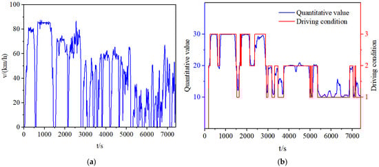
Figure 6.
The dataset and quantitative results of driving conditions. (a) Driving condition data: 0–2786 s represents the driving condition where the dataset is classified as plain highway; 2875–5209 s represents the driving condition where the dataset is classified as hilly highway; 5209–7406 s represents the driving condition where the dataset is classified as national road. (b) Quantitative results of driving conditions.
3.3. Regenerative Braking Qualification Conditions and Determination of Logic Design
The startup threshold for regenerative braking in pure electric commercial vehicles is subject to multiple constraints such as structural limitations, component performance, safety thresholds, and regulatory requirements. For rear-wheel drive models, the power transmission layout determines that the motor can only exert braking force on the rear axle, while the kinetic energy of the front axle dissipates through friction braking as heat energy, resulting in a 30–40% loss of recoverable energy. The performance of core components sets strict boundaries: limited by the rated power of the motor and the charging and discharging capacity of the battery, the recoverable braking torque does not exceed 50% of the maximum braking force, and the recovery efficiency significantly decreases as the braking intensity increases; when the state of charge of the battery exceeds 90%, the regenerative power needs to be limited to prevent overcharging. Additionally, in high-speed or emergency braking conditions, to ensure that braking stability and comply with ECE regulations and GB 12676-2014 standards [28], energy recovery must be completely disabled to ensure braking stability [31]. These multiple constraints collectively form the core content of the entry conditions for regenerative braking.
The distribution strategy for the required braking torque is closely related to the braking intensity z. Based on extensive experimental testing conducted by Dongfeng Liuzhou Motor Co., Ltd., the maximum braking strength zmax for the heavy-duty commercial vehicle in this study is taken as 0.5. In this paper, the normalized braking intensity is adopted as shown in Equation (12):
where Factualbrk is the actual braking force applied to the vehicle and Fmaxbrk is the maximum achievable braking force. The actual maximum braking intensity is z. In the low braking intensity range (z′ < 0.3), the system prioritizes the use of motor braking to meet the demand, thereby maximizing energy recovery efficiency. As the braking intensity increases (0.3 ≤ z′ < 0.7), a hybrid electromechanical braking mode is adopted, where the proportion of motor braking torque is dynamically adjusted to achieve optimal distribution. Under high braking intensity conditions (z′ ≥ 0.7), to ensure braking performance, the motor braking is completely disabled, and the system switches to pure mechanical braking mode with ABS intervention. This strategy ensures braking safety while optimizing energy recovery efficiency. The condition for entering energy recovery mode is set as z′ ≤ 0.7.
The braking performance of the drive motor is closely related to vehicle speed, as motor speed varies linearly with it. Under low-speed conditions, insufficient motor rpm leads to the following issues: a weak back electromotive force, significantly reducing power generation efficiency; and; excessive braking torque that may exceed the structural limits of the motor. In high-speed scenarios, the motor operates in a constant power region, where the available braking torque decays hyperbolically as speed increases, while the risk of braking instability also rises. To balance efficiency and safety under these constraints, the system defines a speed-based operational window within which regenerative braking is permitted. Accordingly, the speed condition for entering energy recovery mode is set as follows: 1.39 m/s ≤ v ≤ 20.83 m/s (5 km/h ≤ v ≤ 75 km/h).
The SOC of a battery is a key parameter indicating the energy reserve of an energy storage system, and its variation directly influences the operational characteristics of the battery. Specifically, the SOC level exhibits a nonlinear negative correlation with internal resistance and also determines the stable range of the open-circuit voltage. These electrochemical characteristics cause the battery’s charge and discharge power capabilities to change dynamically with SOC. When the SOC exceeds a safe threshold, the Battery Management System will forcibly limit the charge and discharge current to protect the battery. In the context of regenerative braking, the real-time SOC is the primary condition for determining whether energy recovery can be activated. To prevent overcharging, the SOC condition for entering regenerative braking mode is set as: SOC ≤ 0.9.
In addition to SOC, battery temperature is also monitored to ensure safe operation. The temperature condition for entering regenerative braking mode is set as T ≤ 45 °C. If the battery temperature exceeds this threshold, the regenerative braking power is curtailed or suspended to prevent overheating and protect battery health.
The vehicle braking control strategy is implemented as follows: First, the required braking torque is calculated based on vehicle state parameters and a driver model, while the maximum braking capacity of the motor at the current speed is evaluated using the motor speed provided by the vehicle state. The system then comprehensively determines whether the conditions for energy recovery are satisfied using multiple parameters—vehicle speed v, braking intensity z, battery SOC SOC, and driving condition quantization parameter d.
If the conditions are met, the system enters energy recovery mode, where the regenerative braking torque and pneumatic braking are coordinated according to an optimized distribution strategy. Otherwise, it switches to pure mechanical braking mode, controlling the pneumatic braking system based on the ideal braking force distribution curve, with the motor braking torque output set to zero. The process is illustrated in Figure 7.
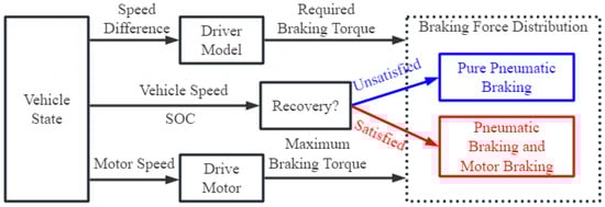
Figure 7.
Braking control strategy decision flowchart. The red path indicates the regenerative braking mode, where motor braking is coordinated with pneumatic braking when conditions are satisfied. The blue path indicates the pure pneumatic braking mode, activated when regenerative conditions are not met.
The torque control strategy under satisfied energy recovery conditions can be summarized as follows:
In the equation, Tf is the mechanical braking torque of the front axle, Tm is the motor braking torque, k is the regenerative braking ratio coefficient output by the control strategy, Tr is the mechanical braking torque of the rear axle, and Treq is the required braking torque during actual braking.
When the energy recovery conditions are not met, the motor does not participate in braking. The braking torque of the rear axle is entirely composed of mechanical braking.
3.4. Fuzzy Control Strategy
To address the significant response delay and high operational complexity issues in the braking systems of heavy commercial vehicles, we adopted a fuzzy logic control strategy to manage the energy flow.
3.4.1. Establishing Membership Functions
A fuzzy logic controller is designed to convert the proportional coefficient k of the motor driving torque into a dynamically tuned output. The inputs to this controller include vehicle speed, braking intensity, SOC, and quantified driving condition parameters. The membership functions, calibrated using substantial experimental data and empirical knowledge, are defined in Figure 8. This calibration aims to optimize the compromise between energy recovery efficiency and braking smoothness while guaranteeing smooth modal transitions. Consequently, the method delivers a favorable balance of precision and real-time performance, rendering it well suited for implementation on embedded systems with limited computing resources.
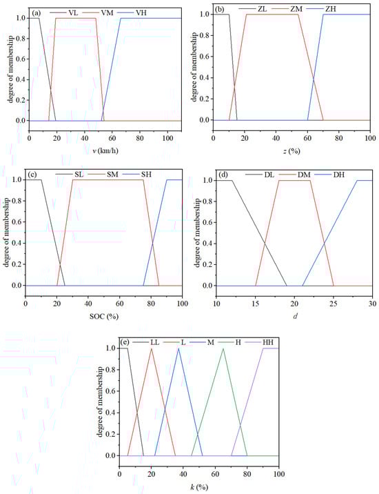
Figure 8.
Membership functions for (a) vehicle speed v (VL: Low, VM: Medium, VH: High), (b) braking intensity z (ZL: Low, ZM: Medium, ZH: High), (c) SOC (SL: Low, SM: Medium, SH: High), (d) driving condition quantization parameter d (DL: Plain Highway, DM: Hilly Highway, DH: National Road), and (e) motor braking torque ratio coefficient k (LL: Very Low, L: Low, M: Medium, H: High, HH: Very High).
3.4.2. Fuzzy Rule Base
The fuzzy rule base is a collection of a series of fuzzy inference rules within the fuzzy controller, which is the core of its design and directly determines the control performance of the entire system. Based on existing research and empirical data obtained from the tests conducted by Dongfeng Liuzhou Automobile Co., Ltd., this study integrates the influence laws of braking intensity, vehicle speed, battery state of charge, and driving conditions on energy recovery efficiency. The fuzzy inference is completed using the center-of-gravity method, and a total of 81 fuzzy rules are established. The rules for different driving conditions correspond to plain highways, hilly highways, and national road scenarios, as shown in Table 2, Table 3 and Table 4, respectively.
Table 2.
Fuzzy Rules for the Plain Highway Condition.
Table 3.
Fuzzy Rules for the Hilly Highway Condition.
Table 4.
Fuzzy Rules for the National Road Condition.
3.5. Vehicle Model Development
The simulation model was developed in the MATLAB/Simulink (R2020a) environment. The Fuzzy Logic Toolbox was utilized to design and implement the fuzzy inference system described in Section 3.4. The vehicle longitudinal dynamics, powertrain components, and control strategy were integrated into a co-simulation framework. The driving cycle input module provides target speed signals that define the driving requirements, which are then processed by the driver module to generate corresponding pedal signals and feedback control signals, emulating driver behavior and coordinating dynamic response. The vehicle module receives these pedal and control signals, converts them into vehicle state signals, and forwards them to the control strategy module. Based on the received state and feedback signals, the control strategy module dynamically optimizes the energy management strategy to ensure efficient and stable vehicle operation. The detailed architecture of the model is presented below Figure 9. The vehicle parameters are listed in Table 5.
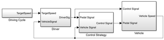
Figure 9.
Simulink model.
Table 5.
Key Parameters for Simulation Model.
3.5.1. Vehicle Longitudinal Dynamics Model
The vehicle dynamics modeling in this study focuses on the longitudinal dynamics of the electric powertrain, employing a simplified single-degree-of-freedom model to represent the overall vehicle motion [32]. The force balance equation for longitudinal vehicle motion is given by Equation (14):
In the equation, F is the driving force required during vehicle operation; m is the total vehicle mass; α is the road slope; CD is the air resistance coefficient; A is the vehicle’s frontal area; v is the vehicle speed; δ is the rotational mass conversion factor; fr is the rolling resistance coefficient.
3.5.2. Electric Motor Model
Drive motors typically operate in two modes: the motor mode and the generator mode. When the vehicle is driving, the motor operates in motor mode, converting electrical energy into mechanical energy to output the corresponding driving torque that propels the vehicle. When the vehicle is braking and the conditions for braking energy recovery are met, the motor switches to generator mode, converting mechanical energy back into electrical energy. In this mode, the kinetic energy of the vehicle is transformed through motor reversal into electrical energy for storage. The development of the motor model must accurately capture these input–output characteristics. The external performance of the drive motor can be described by Equation (15).
In the equation, Tmax represents the maximum output torque of the drive motor, Tm denotes the peak torque of the drive motor, Pmax indicates the peak power of the drive motor, n refers to the actual rotational speed of the drive motor, and n0 is the base speed of the drive motor. The external characteristic curve of the drive motor is illustrated in Figure 10.
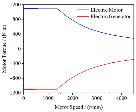
Figure 10.
External characteristic curve of drive motor.
As the drive motor operates in motoring mode, the motor output torque Tm > 0. The calculation formula for the drive motor power Pm is as follows:
When the drive motor operates as a generator, the motor output torque Tm < 0. The calculation formula for the drive motor power Pm is as follows:
As indicated in Equations (16) and (17), the power output of the motor depends not only on speed and torque but is also influenced by motor efficiency. The efficiency characteristics of the drive motor are illustrated in Figure 11.
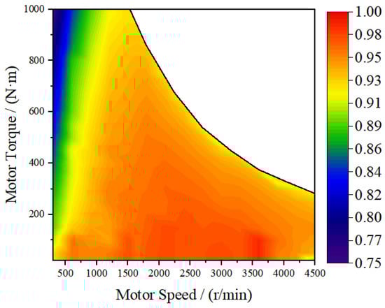
Figure 11.
Drive Motor Efficiency MAP.
As can be seen from the figure, the color of the contours represents different levels of motor efficiency, with redder hues indicating higher efficiency. The efficiency value corresponding to any given motor speed and torque can be obtained through interpolation. Since the efficiency characteristics in both operational modes of the motor—motoring and generating—are essentially symmetric, similar to its external performance, only the efficiency map for the drive mode is shown here.
3.5.3. Battery Model
This work utilizes a simplified internal resistance battery model [33]. The equivalent circuit diagram of the battery internal resistance model is shown in Figure 12.
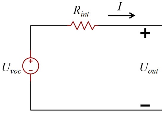
Figure 12.
Equivalent Circuit Diagram of the Battery Internal Resistance Model.
Based on the equivalent circuit diagram of the battery and Kirchhoff’s laws, the state equation of the battery is formulated as shown in Equation (18):
In the equation, Rint is the internal resistance of the battery, I is the battery current, Uvoc is the voltage of the ideal voltage source, i.e., the open-circuit voltage of the battery, Uout is the output voltage of the voltage source, i.e., the actual output voltage of the battery.
The SOC is estimated using the Ampere-hour integration method, with the calculation formula given as follows:
In the equation, SOC0 is the initial state of charge, I(t) is the time-varying current, η(T) is the Coulombic efficiency related to battery temperature, and Cb is the rated capacity of the battery. The operational mode of the drive motor determines the battery’s SOC. When operating as a motor, the battery provides power, leading to a decrease in SOC. When functioning as a generator, the motor delivers a charging current, consequently increasing the SOC. A critical limitation of the Ampere-hour integration method is its strong dependence on the initial SOC value.
Battery heat generation during charging consists of irreversible Joule heat and reversible reaction heat. The resulting temperature increase is calculated using Equation (20).
where η is the heat generation efficiency. The terms m and Cp denote the battery mass and specific heat capacity, respectively. T0 and T represent the initial (set to 25 °C) and final temperatures.
4. Results and Discussion
In this study, two core strategies—the fuzzy control strategy and the driving condition recognition-based control strategy—were embedded into the Simulink vehicle model. To verify the rationality of these strategies, two types of operating conditions were adopted: the collection of actual vehicle test scenarios and the double-WTVC conditions. The collection of actual vehicle test scenarios (hereinafter referred to as the ‘Actual Scenario Collection’). This test cycle was constructed by selecting and concatenating representative driving segments from the real-world operational dataset [28] to simulate the complex road conditions encountered in real logistics transportation. These segments are integrated based on road conditions to form continuous test scenarios, which are used to simulate the complex road conditions encountered in real logistics transportation and to verify the actual adaptability of the strategies.
For the evaluation of braking safety, the matching relationship between the utilization adhesion coefficients of the front and rear axles and the braking intensity was analyzed. The comparative results of the utilization adhesion coefficients for both axles are shown in Figure 13.
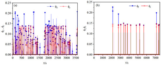
Figure 13.
Comparison of utilization adhesion coefficients between front and rear axles: (a) Double WTVC. (b) Test scenarios.
As shown in Figure 13, under the proposed strategy, the utilization adhesion coefficient of the front axle is generally greater than that of the rear axle. This design helps prevent the rear wheels from locking up before the front wheels, thereby avoiding potential loss of vehicle control.
Online condition recognition assumes that the driving condition remains relatively stable over a recent time window. The underlying principle is illustrated in Figure 14.
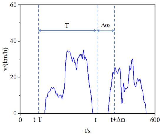
Figure 14.
Schematic Diagram of Online Condition Recognition.
We employed a sliding time window approach for condition recognition, with an identification cycle T of 180 s and a prediction horizon △ω of 5 s. Based on historical vehicle speed data within the time window T, the method predicts the short-term driving condition category under the assumption that conditions remain relatively stable over a limited period.
A simulation test was conducted under twice the WTVC and the test scenarios, assuming correct initial cycle recognition. The results, presented in Figure 15, show that the condition recognition model closely follows the actual variations. The high recognition accuracy thus verifies the model’s feasibility for collaborative use with the vehicle dynamics model and the regenerative braking strategy.
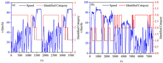
Figure 15.
Online Condition Recognition Performance: (a) Double WTVC. (b) Test scenarios.
4.1. Full Vehicle Model Simulation Results
A comparative simulation was conducted to evaluate the improvement effect of the proposed strategy in regenerative braking energy recovery. Two strategies were tested: strategy one is the proposed strategy based on condition recognition, and strategy two is a benchmark strategy without condition recognition. The SOC curves of the two strategies under different driving conditions are shown in Figure 16.
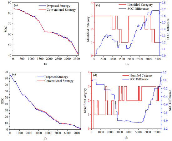
Figure 16.
Comparison of two strategies for SOC: (a) Variation in SOC under double WTVC. (b) Difference in SOC between the two strategies under double WTVC. (c) Variation in SOC under the test scenarios. (d) Difference in SOC between the two strategies under the test scenarios.
The simulation results indicate that the SOC of the power battery under both regenerative braking strategies generally exhibits a decreasing trend, albeit with several minor rebounds. These fluctuations confirm that braking energy recovery was successfully activated multiple times during the driving cycle. As illustrated in Figure 16b,d, a comparative analysis of the SOC difference between the two strategies, combined with the identified driving conditions, reveals that the proposed adaptive strategy dynamically adjusts the energy recovery intensity based on real-time driving condition recognition and the fuzzy rules derived in Section 3.4. Specifically, under national road conditions, the system automatically switches to a recovery mode with 30% higher regenerative torque than plain highway conditions, significantly increasing the electric braking force. In contrast, under plain high-speed conditions, a conservative recovery mode is adopted to prioritize driving safety, adhering to the braking force distribution constraints outlined in Equation (9). Accordingly, the SOC difference between the two strategies increases noticeably in national road and hilly high-speed scenarios, whereas it remains relatively small in plain high-speed conditions due to the imposed safety constraints. Ultimately, Strategy one achieves a higher final SOC retention rate than Strategy two, demonstrating the effectiveness of the condition-based regenerative braking strategy in optimizing energy efficiency. This adaptive mechanism not only enhances energy recovery but also ensures a coordinated balance between energy retrieval and braking stability by aligning with the safety requirements of different driving conditions.
As shown in Table 6, under the double WTVC, Strategy One achieved a total energy recovery of 71,244 kJ, corresponding to a 5.8% increase in the net energy recovered by the battery SOC compared to Strategy Two. A condition-specific analysis reveals that Strategy One adopted a more aggressive approach on national and hilly highways, enhancing energy recovery by 9.4% and 6.0%, respectively. In contrast, it operated more conservatively on plain highways, reducing recovery by 6.8% to prioritize safety.
Table 6.
Energy Recovery Comparison under Double-WTVC Conditions.
As shown in Table 7, under the test scenarios, Strategy One achieved a total energy recovery of 78,393 kJ. A condition-specific analysis reveals that Strategy One adopted a more aggressive approach on national, enhancing energy recovery by 24.3%, respectively. In contrast, it operated more conservatively on plain highways and hilly highways, reducing recovery by 31% and 1.1% to prioritize safety. These results collectively verify the effectiveness and adaptability of the proposed strategy.
Table 7.
Energy Recovery Comparison under Actual Vehicle Test Scenarios.
4.2. Control Strategy HIL Testing
To verify the real-time performance of the developed control strategy, HIL simulation was carried out following the offline analysis. The control performance in these two environments was compared, serving as a critical step toward full vehicle validation.
An HIL platform was configured for experimental validation. The setup revolved around a dSPACE real-time simulator which executed a closed-loop vehicle plant model inclusive of an automated driver module. This configuration, running under standardized driving profiles, ensured repeatable testing conditions devoid of manual variances. The target vehicle controller, hosting the regenerative braking strategy, was interfaced with the simulator through a CAN communication network. All experimental operations, from test initiation to data acquisition, were centralized via the ControlDesk 7.1 interface on a master host computer. The HIL test platform used in this study is shown in Figure 17.
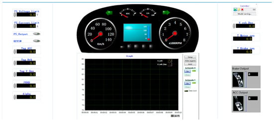
Figure 17.
Hardware in Loop Test Platform.
Taking the HIL results under the double WTVC and the test scenarios as an example, the speed tracking performance is illustrated in Figure 18.
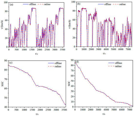
Figure 18.
Speed Tracking Curves and Error Profiles Under Different Driving Conditions: (a) Speed tracking curves under double-WTVC driving conditions. (b) Speed tracking curves under the test scenarios. (c) SOC under double-WTVC driving conditions. (d) Speed tracking error profile under the test scenarios.
As illustrated in Figure 18, the actual vehicle speed demonstrated superior tracking performance relative to the reference speed during the HIL test. To quantitatively evaluate this tracking capability, we employed a modified symmetric mean absolute percentage error metric, defined in Equation (21). A normalization constant of 1 km/h was incorporated into the denominator to mitigate exaggerated error values in the extremely low-speed range.
Using Equation (21), the error under the WTVC and the test scenarios was calculated to be 1.23% and 2%, respectively, and the maximum speed errors were 0.96 km per hour and 2.07 km per hour, respectively. These results indicate that the accuracy meets the requirements of the simulation.
5. Conclusions and Future Work
This study developed an intelligent regenerative braking strategy for heavy-duty electric logistics vehicles by integrating LVQ-based driving condition recognition with adaptive fuzzy control. The proposed system dynamically adapts to three predominant real-world road types (plain highway, hilly highway, and national road) and achieved a 5.8% improvement in net energy recovery compared to a non-adaptive benchmark, while strictly complying with braking safety regulations. The feasibility of real-time implementation was confirmed through HIL tests.
The current work validates the strategy under specific regional driving cycles and constant component efficiency assumptions. To address these limitations and explore broader impacts, future research will focus on the following:
(1) System Robustness and Durability Analysis: Investigating the strategy’s long-term effects on brake pad wear dynamics and chassis stress under diverse braking conditions. (2) Generalizability Enhancement: Integrating predictive map and traffic information for proactive energy management across different regions. (3) Adaptive Component Modeling: Incorporating models of battery and motor aging to maintain performance over the vehicle’s lifecycle. (4) Integrating battery thermal dynamics and advanced state-of-charge estimation: Developing a coupled SOC–temperature model to refine overcharge and overheat prevention strategies, enhancing both safety and battery lifespan.
Author Contributions
Conceptualization, X.F., H.Z. and W.M.; methodology, H.Z.; software, W.M. and D.P.; validation, X.F., H.Z. and W.M.; formal analysis, H.Y. and Y.L.; investigation, W.M.; resources, Y.L. and D.P.; data curation, W.M. and D.P.; writing—original draft preparation, W.M. and H.C.; writing—review and editing, H.Z.; visualization, W.M.; supervision, H.C.; project administration, W.M. and H.Z.; funding acquisition, X.F. and D.P. All authors have read and agreed to the published version of the manuscript.
Funding
This research was funded by “Guangxi Science and Technology Project”, grant number “2024GXNSFBA010261, 2023GXNSFFA026002, AD22080042, AB21220052, and AD23026117”.
Data Availability Statement
The driving cycle dataset used in this study is publicly available on GitHub at https://github.com/momowl-studying/Preprocessing-of-Southwest-Heavy-Truck-Driving-Data. (accessed on 10 December 2025).
Conflicts of Interest
Yongqiang Lv is employees of Guangxi Shubo Technology Co., Ltd. and Defeng Peng is employees of Dongfeng Liuzhou Motor Co., Ltd. The remaining authors declare that the research was conducted in the absence of any commercial or financial relationships that could be construed as a potential conflict of interest.
Abbreviations
The following abbreviations are used in this manuscript:
| LVQ | Learning Vector Quantization | |
| WTVC | World Transient Vehicle Cycle | |
| SOC | State of Charge | |
| RBS | Regenerative Braking System | |
| RFE | Recursive Feature Elimination | |
| HIL | Hardware-in-the-loop | |
| Variables | Description | Unit |
| v | Vehicle speed | Km/h |
| z | Braking intensity | \ |
| β | Braking force distribution coefficient | \ |
| α | Learning rate (LVQ) | \ |
| Tm | Motor braking torque | N·m |
| Tf | Front-axle braking torque | N·m |
| Tr | Rear-axle braking torque | N·m |
| Treq | Required braking torque | N·m |
| η | Motor efficiency | \ |
| k | Regenerative braking ratio coefficient | \ |
| d | Driving condition quantization parameter | \ |
| a, b | Distance from CG to front/rear axle | m |
| L | Wheelbase | m |
| hg | Height of center of gravity | m |
| φf, φr | Utilization adhesion coefficient (front/rear) | \ |
References
- State Post Bureau of China. Global Express Development Report; Development Research Center of State Post Office: Beijing, China, 2019.
- Jiang, X.; Guo, X. Evaluation of performance and technological characteristics of battery electric logistics vehicles: China as a case study. Energies 2020, 13, 2455. [Google Scholar] [CrossRef]
- Ma, Z.; Sun, D. Energy recovery strategy based on ideal braking force distribution for regenerative braking system of a four-wheel drive electric vehicle. IEEE Access 2020, 8, 136234–136242. [Google Scholar] [CrossRef]
- Zhang, J.; Lv, C.; Gou, J.; Kong, D. Cooperative control of regenerative braking and hydraulic braking of an electrified passenger car. Proc. Inst. Mech. Eng. Part D J. Automob. Eng. 2012, 226, 1289–1302. [Google Scholar] [CrossRef]
- Patil, L.N.; Khairnar, H.P. Assessing Impact of Smart Brake Blending to Improve Active Safety Control by Using Simulink. Appl. Eng. Lett. 2021, 6, 29–38. [Google Scholar] [CrossRef]
- Qin, Y.; Zheng, Z.A.; Chen, J. Dual-Fuzzy Regenerative Braking Control Strategy Based on Braking Intention Recognition. World Electr. Veh. J. 2024, 15, 524. [Google Scholar] [CrossRef]
- Van Meldert, B.; De Boeck, L. Introducing Autonomous Vehicles in Logistics: A Review from a Broad Perspective; Working Papers of Department of Decision Sciences and Information Management, Leuven; KU Leuven: Leuven, België, 2016; p. 543558. [Google Scholar]
- Zhu, Y.; Li, X.; Liu, Q.; Li, S.; Xu, Y. A comprehensive review of energy management strategies for hybrid electric vehicles. Mech. Sci. 2022, 13, 147–188. [Google Scholar] [CrossRef]
- Shen, P.; Zhao, Z.; Zhan, X.; Li, J.; Guo, Q. Optimal energy management strategy for a plug-in hybrid electric commercial vehicle based on velocity prediction. Energy 2018, 155, 838–852. [Google Scholar] [CrossRef]
- Chen, J.; Yu, J.; Zhang, K.; Ma, Y. Control of regenerative braking systems for four-wheel-independently-actuated electric vehicles. Mechatronics 2018, 50, 394–401. [Google Scholar] [CrossRef]
- Hamada, A.T.; Orhan, M.F. An Overview of Regenerative Braking Systems. J. Energy Storage 2022, 52, 105033. [Google Scholar] [CrossRef]
- Garg, B.D.; Cadle, S.H.; Mulawa, P.A.; Groblicki, P.J.; Laroo, C.; Parr, G.A. Brake wear particulate matter emissions. Environ. Sci. Technol. 2000, 34, 4463–4469. [Google Scholar] [CrossRef]
- Hicks, W.; Green, D.C.; Beevers, S. Quantifying the change of brake wear particulate matter emissions through powertrain electrification in passenger vehicles. Environ. Pollut. 2023, 336, 122400. [Google Scholar] [CrossRef] [PubMed]
- Zhang, Z.; Dong, Y.; Han, Y. Dynamic and Control of Electric Vehicle in Regenerative Braking for Driving Safety and Energy Conservation. J. Vib. Eng. Technol. 2020, 8, 179–197. [Google Scholar] [CrossRef]
- Yang, Y.; He, Q.; Chen, Y.; Fu, C. Efficiency Optimization and Control Strategy of Regenerative Braking System with Dual Motor. Energies 2020, 13, 711. [Google Scholar] [CrossRef]
- Li, S.; Yu, B.; Feng, X. Research on Braking Energy Recovery Strategy of Electric Vehicle Based on ECE Regulation and I Curve. Sci. Prog. 2020, 103, 0036850419877762. [Google Scholar] [CrossRef]
- Ziadia, M.; Kelouwani, S.; Amamou, A.; Agbossou, K. Weather-Adaptive Regenerative Braking Strategy Based on Driving Style Recognition for Intelligent Electric Vehicles. Sensors 2025, 25, 1175. [Google Scholar] [CrossRef]
- Li, Q.; Huang, W.; Chen, W.; Yan, Y.; Shang, W.; Li, M. Regenerative Braking Energy Recovery Strategy Based on Pontryagin’s Minimum Principle for Fuel Cell/Supercapacitor Hybrid Locomotive. Int. J. Hydrogen Energy 2019, 44, 5454–5461. [Google Scholar] [CrossRef]
- Yang, X.; Wang, Y.; Liu, D. The Series Control Strategy of Regenerative Braking for Range Extender Electric Vehicles. Control Eng. China 2018, 25, 238–244. [Google Scholar]
- Liang, J.; Walker, P.D.; Ruan, J.; Yang, H.; Wu, J.; Zhang, N. Gearshift and Brake Distribution Control for Regenerative Braking in Electric Vehicles with Dual Clutch Transmission. Mech. Mach. Theory 2019, 133, 1–22. [Google Scholar] [CrossRef]
- Li, Z.; Khajepour, A.; Song, J. A comprehensive review of the key technologies for pure electric vehicles. Energy 2019, 182, 824–839. [Google Scholar] [CrossRef]
- Mo, W.; Zheng, H. Real-World Driving Cycle Dataset for 18-Ton Heavy-Duty Electric Logistics Trucks in Southwest China. GitHub. 2025. Available online: https://github.com/momowl-studying/Preprocessing-of-Southwest-Heavy-Truck-Driving-Data (accessed on 10 December 2025).
- Ahmed, M.; Seraj, R.; Islam, S.M.S. The k-means Algorithm: A Comprehensive Survey and Performance Evaluation. Electronics 2020, 9, 1295. [Google Scholar] [CrossRef]
- Montazeri-Gh, M.; Ahmadi, A.; Asadi, M. Driving Condition Recognition for Genetic-Fuzzy HEV Control. In Proceedings of the 2008 3rd International Workshop on Genetic and Evolving Systems, Witten-Bommerholz, Germany, 4 March 2008; pp. 65–70. [Google Scholar]
- Luo, Y.T.; Hu, H.F.; Shen, J.J. Driving Condition Analysis and Recognition for Hybrid Electric Vehicles. J. South China Univ. Technol. Nat. Sci. Ed. 2007, 35, 8–13. [Google Scholar]
- Ericsson, E. Independent driving pattern factors and their influence on fuel-use and exhaust emission factors. Transp. Res. Part D Transp. Environ. 2001, 6, 325–345. [Google Scholar] [CrossRef]
- Kohonen, T. Improved Versions of Learning Vector Quantization. In Proceedings of the 1990 IJCNN International Joint Conference on Neural Networks, San Diego, CA, USA, 17–21 June 1990; pp. 545–550. [Google Scholar]
- GB 12676-2014; Road vehicles—Braking systems—Construction, performance and test methods. Standards Press of China: Beijing, China, 2014.
- Verma, P.C.; Menapace, L.; Bonfanti, A.; Ciudin, R.; Gialanella, S.; Straffelini, G. Braking pad-disc system: Wear mechanisms and formation of wear fragments. Wear 2015, 322, 251–258. [Google Scholar] [CrossRef]
- De Zepeda, M.V.N.; Meng, F.; Su, J.; Zeng, X.J.; Wang, Q. Dynamic clustering analysis for driving styles identification. Eng. Appl. Artif. Intell. 2021, 97, 104096. [Google Scholar] [CrossRef]
- Li, X.; Ma, J.; Zhao, X.; Wang, L. Study on Braking Energy Recovery Control Strategy for Four-Axle Battery Electric Heavy-Duty Trucks. Int. J. Energy Res. 2023, 2023, 1868528. [Google Scholar] [CrossRef]
- Yu, Y.; Wang, K.; Fan, Y.; Tang, X.; Huang, M.; Bao, J. Operating Condition Recognition Based Fuzzy Power-Following Control Strategy for Hydrogen Fuel Cell Vehicles (HFCVs). World Electr. Veh. J. 2025, 16, 102. [Google Scholar] [CrossRef]
- Lu, W.Q.; Zhang, C.T.; Wang, J.Q.; Zuo, H.M. Modeling and Simulation of Vehicle Battery Model Based on Simulink. Automob. Appl. Technol. 2019, 8, 10–13. [Google Scholar]


Disclaimer/Publisher’s Note: The statements, opinions and data contained in all publications are solely those of the individual author(s) and contributor(s) and not of MDPI and/or the editor(s). MDPI and/or the editor(s) disclaim responsibility for any injury to people or property resulting from any ideas, methods, instructions or products referred to in the content. |
© 2026 by the authors. Published by MDPI on behalf of the World Electric Vehicle Association. Licensee MDPI, Basel, Switzerland. This article is an open access article distributed under the terms and conditions of the Creative Commons Attribution (CC BY) license.