1. Introduction
In recent years, autonomous driving technology has experienced rapid development. As a critical control task in autonomous systems, path tracking faces an urgent challenge: how to simultaneously achieve tracking accuracy and control smoothness under varying operating conditions.
To address the insufficient utilization of perceptual information, where intelligent vehicles can perceive 100–200 m ahead while real-time Model Predictive Control (MPC) prediction horizons are limited to approximately 30 m, a soft actor-critic (SAC) agent is employed to proactively adjust the MPC weight matrices based on long-range perceptual information. Unlike existing methods that passively adjust weights based on current tracking errors [
1], the proposed approach initiates weight adjustment before the vehicle enters challenging scenarios (e.g., sharp curves, abrupt adhesion variations), thereby achieving smooth transitions [
2]. Both simulation and real-vehicle experiments demonstrate that, compared to fixed-weight MPC, the proposed method reduces lateral tracking errors by 43.4% in lane-change scenarios under docking conditions [
3].
Current path-tracking control methods include PID control, preview control, sliding mode control, fuzzy control, and Model Predictive Control (MPC) [
4], etc. Traditional PID and preview control approaches exhibit limited robustness; sliding mode control is susceptible to chattering phenomena; and fuzzy control relies heavily on expert knowledge. MPC demonstrates superior performance under complex operating conditions by explicitly considering constraints and predictive dynamics. However, MPC with fixed parameters struggles to maintain satisfactory tracking performance and control smoothness when operating conditions change abruptly (e.g., sudden variations in road surface adhesion coefficient) [
5].
To achieve adaptive adjustment of MPC parameters, the existing research has employed methods such as Bayesian optimization and fuzzy control [
6], yet significant limitations persist: heuristic algorithms (PSO [
7], GA [
8]) are prone to local optima and cannot adapt online, and fuzzy control cannot handle operating condition changes beyond predefined rules and exhibits high system complexity. Therefore, an adaptive tuning strategy that is capable of autonomously exploring and learning optimal parameters in response to environmental changes is required.
In recent years, deep reinforcement learning algorithms (DQN [
9], DDPG [
10], TD3 [
11], SAC [
12]) have demonstrated tremendous potential in complex control problems. Among these, the soft actor-critic (SAC) algorithm, based on the maximum entropy reinforcement learning framework, enables more stable policy optimization in continuous action spaces.
When intelligent vehicles encounter sudden changes in the road surface adhesion coefficient during operation, degradation of tracking accuracy and stability is readily induced. To address these issues, an SAC-based adaptive tuning strategy for MPC parameters is designed in this paper. A linear time-varying (LTV) MPC controller is constructed based on a three-degree-of-freedom vehicle dynamics model, with an SAC agent employed to tune the weighting matrix parameters (, , ) in real-time, thereby preventing control performance degradation. The reward function comprehensively considers metrics including tracking accuracy, control smoothness, error improvement, and dual-objective achievement, while incorporating an adaptive smoothness weighting mechanism to achieve dynamic balance. Through simulations of double-lane-change maneuvers under normal and transitional operating conditions, as well as experimental validation of double-lane-change maneuvers, the proposed method significantly maintains the tracking accuracy, thereby enhancing the overall control quality.
The main innovations of this study are reflected in the following aspects: First, differently from the existing passive adjustment methods based on current tracking errors, this paper proposes an active weight adjustment strategy that leverages the long-range perception information of intelligent vehicles to compensate for the limitation of the finite MPC prediction horizon. This enables parameter tuning to be initiated in advance before the vehicle enters nonlinear working conditions, thus achieving a smoother transition. Second, an adaptive framework based on SAC is developed, which can autonomously learn the optimal MPC weight matrix (, , ) for varying working conditions. This framework overcomes the limitations of heuristic algorithms that tend to fall into local optima and rule-based methods with limited generalization ability. Third, a reward function comprehensively considering tracking accuracy and error improvement is designed, and an adaptive smoothness weight mechanism is introduced to realize the dynamic balance of multiple competing objectives in different scenarios. Finally, the effectiveness of the proposed method is rigorously verified through simulation studies covering normal and docking working conditions as well as real-vehicle experiments, which demonstrates that significant improvements are achieved in both tracking accuracy and control quality.
2. Vehicle Dynamics Model
Based on a three-degree-of-freedom vehicle dynamics model, the dynamics equations are established by considering lateral, longitudinal, and yaw motions [
13]:
where
denotes the vehicle mass;
represent the longitudinal and lateral displacements of the vehicle, respectively;
and
characterize the longitudinal and lateral velocities of the vehicle, respectively;
is the vehicle yaw angle and
represents the yaw rate;
denotes the moment of inertia of the vehicle about the z-axis;
and
represent the distances from the center of gravity to the front and rear axles, respectively;
denotes the front wheel steering angle;
and
are the longitudinal forces of the front and rear wheels, respectively; and
and
are the lateral forces of the front and rear wheels, respectively.
Tire Force Model
A nonlinear tire model is selected to enhance the simulation accuracy. The Pacejka model (also known as the Magic Formula) is a semi-empirical, semi-theoretical model that integrates both empirical evidence and theoretical foundations. It is capable of simulating both linear and nonlinear tire characteristics, while effectively characterizing the steady-state mechanical behavior of tires. The tire lateral force equation is expressed as follows:
where
D represents the peak factor; C denotes the shape factor; B is the stiffness factor; E represents the curvature factor; and
denotes the tire slip angle.
3. MPC-Based Path Tracking Controller
Compared with the nonlinear model, the linear time-varying model offers greater computational simplicity and efficiency, while possessing excellent real-time processing capability. Therefore, the nonlinear vehicle dynamics model in this paper is linearized to obtain the linear time-varying Equation (3) [
14]:
where
represents the system state variables;
(front wheel steering angle) denotes the system control input; and
.
To achieve lateral tracking of the target path by the vehicle, the system output is defined as the lateral position and heading angle:
After discretizing the linear time-varying equation using the first-order forward difference method, the following discrete state–space equation is obtained:
where
, and T represents the sampling period.
After introducing the incremental model, the following is obtained:
Prediction Equation
The prediction equation constitutes a crucial component of Model Predictive Control (MPC), as it is required to compute the system output over a future time horizon. First, Equation (6) is transformed into the following: .
Thus, a new state-space expression is obtained:
where
where
, and the system output is a two-dimensional vector
.
According to the fundamental principles of Model Predictive Control (MPC), let
denote the prediction horizon and
denote the control horizon, where
. The system output at time instant k is defined as follows:
Define the system input at time step k as follows:
Based on the fundamental theoretical framework of Model Predictive Control (MPC), the prediction equation for the system at future time instant k can be constructed as follows:
where
The inherent complexity of the vehicle dynamics model, coupled with the multiple constraints introduced in the system, significantly increases the difficulty of solving the optimization problem. To reduce computational complexity and ensure real-time performance, a slack variable, ε, is introduced into the objective function design. Based on the existing literature, the objective function is formulated as follows:
where
characterizes the deviation between the actual output and the reference path;
and R belong to the weighting matrices; when the system tracking error is small, larger values are selected to enable the vehicle to track the preceding vehicle smoothly and without error; and when the system tracking error is large, smaller values are selected to ensure vehicle driving safety.
represents the weighting coefficient of
. Based on the above content, this problem can be transformed into a quadratic programming problem for solution [
15].
Based on the above content, this problem can be transformed into a quadratic programming problem, namely:
4. SAC-Based Adaptive Parameter Tuning Strategy
4.1. SAC Algorithm Procedure
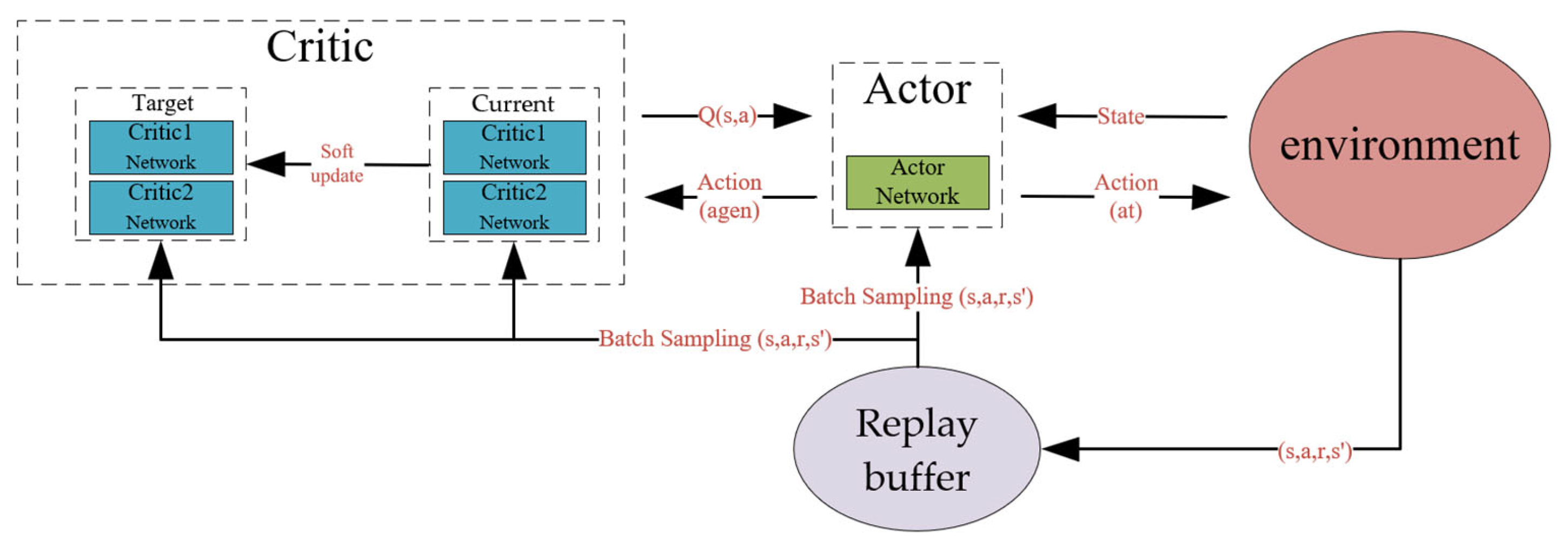
To address the controller performance degradation caused by variations in road surface adhesion conditions, vehicle velocity, and road curvature under the diverse operating conditions of intelligent vehicles, an SAC-based adaptive parameter-tuning strategy for MPC is proposed in this paper. Compared with DDPG and TD3, SAC possesses the following advantages: first, SAC employs a stochastic policy rather than a deterministic policy, whereby the policy itself is inherently exploratory without requiring additional exploration noise; second, through entropy regularization, diversity in the policy is encouraged, thereby improving sample efficiency and training stability; and finally, SAC incorporates an automatic temperature adjustment mechanism that adaptively balances exploration and exploitation, endowing the algorithm with superior generalization capability across different tasks [
16]. The flowchart of the SAC algorithm is illustrated in
Figure 1.
The SAC algorithm procedure is presented in Algorithm 1 [
16].
| Algorithm 1: SAC Adaptive Parameter Tuning Algorithm |
Initialize the Actor network with parameters Initialize Critic networks and with parameters , Initialize target Critic networks and with ← , ← Initialize temperature parameter α (automatic tuning enabled) Initialize replay buffer D with capacity N for episode = 1, 2, …, M do - (a)
Initialize exploration noise N and obtain initial state s1 - (b)
for time step t = 1, 2, …, T do - (c)
Sample action from the policy network - (d)
Execute action at and observe reward rt and next state st+1 - (e)
Store transition in replay buffer D - (f)
Sample a random minibatch of transitions from D - (g)
Sample next action - (h)
Compute target Q-value: - (i)
Update Critic networks by minimizing: - (j)
if delayed update condition satisfied then - (k)
Sample action under current policy - (l)
Update Actor network by maximizing: - (m)
Perform soft update of target networks: - (n)
end if
end for end for
|
4.2. State Space Design
4.2.1. State Vector Definition
The SAC state vector is designed as a 10-dimensional vector:
where
and
represent the lateral error and heading error, respectively;
and
denote the error change rates;
and
represent the longitudinal and lateral velocities, respectively;
denotes the yaw rate;
represents the sideslip angle at the center of gravity;
denotes the road surface adhesion coefficient (ranging from 0.4 to 0.8); and
represents the rate of change in the adhesion coefficient.
4.2.2. State Normalization
To enhance training efficiency and convergence, an online normalization method is employed to standardize the states:
where
represents the moving average of the i-th dimensional state;
denotes the moving variance of the i-th dimensional state; and
is a numerical stability term.
4.3. Action Space Design
Action Vector Definition
In this paper, the control horizon
and the prediction horizon
are set as constant values, and the action vector of SAC is defined as the scaling factors (rather than direct weight values) of the MPC weight parameters as
. The MPC weight values are determined as follows:
The adaptive weights are obtained by multiplying the scaling factors of the MPC weight parameters with the error weights and constraint weights of the MPC.
4.4. Reward Function Design
The reward function constitutes the core of reinforcement learning and directly determines the optimization objective of the agent. In this study, to ensure real-time control performance in experimental validation, the parameters of the reward function are manually configured. The current reward parameters have been demonstrated to achieve the desired objectives. The reward function designed in this paper comprehensively considers tracking accuracy, control smoothness, vehicle stability, and environmental adaptability. The specific form can be expressed as follows:
The detailed design of each reward component is as follows:
- (1)
Lateral tracking reward
(primary optimization objective with the largest weight): A piecewise stepwise reward is adopted to reinforce the value of small errors, categorized as excellent, good, satisfactory, passing, fair, and unsatisfactory.
- (2)
Heading tracking reward
(secondary objective with reduced weight):
- (3)
Control smoothness penalty: , where represents the steering angle increment.
- (4)
Vehicle stability penalty: , which penalizes excessive sideslip angles to ensure vehicle stability.
- (5)
Error improvement reward
:
- (6)
Special reward for friction coefficient transition region
is designed specifically for the road surface adhesion coefficient transition zone (95 m < x < 105 m):
When , .
- (7)
Speed maintenance penalty: .
- (8)
Low-friction road stability reward :
When , .
- (9)
Hyperparameter settings are listed in
Table 1.
4.5. Design of Scaling Factors and Robustness Analysis
A piecewise stepped reward mechanism is adopted for the reward function in this paper, which is designed in accordance with the piecewise setting of error thresholds, and the corresponding reward values are assigned based on the requirements for lateral tracking accuracy. These thresholds are determined according to the lateral control accuracy specifications for autonomous driving. In addition, the scaling factors for MPC weight parameters exhibits an exponential decay characteristic, which can effectively guide the policy network to optimize towards high-precision tracking.
Moreover, the smoothness weight is adaptively adjusted based on the tracking error: when the error is small, control smoothness is emphasized to avoid unnecessary chattering; when the error is large, tracking accuracy is prioritized. This mechanism achieves a dynamic balance between accuracy and smoothness.
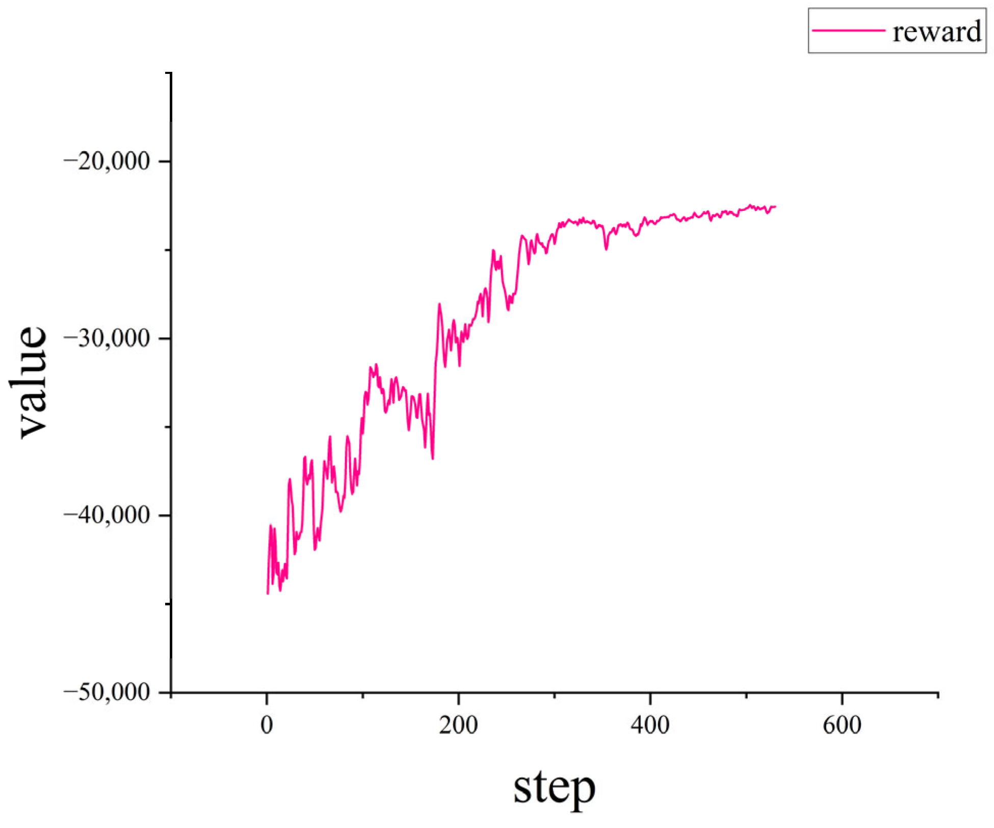
During training, the scaling weights for lateral error, heading error, and steering constraint are set to the ranges of [0.5, 4.0], [0.5, 2.5], and [0.5, 2.5], respectively. The training curve of the reward function is illustrated in
Figure 2, with the total training time being approximately 4.5 h.
Furthermore, owing to the soft constraint mechanism employed by the SAC algorithm, natural fluctuations in the scaling factors occur during the training process. The range of such fluctuations covers and even exceeds the perturbation range of ±20%, thus ensuring the strong robustness of the reward function design.
Compared with the traditional MPC controller with fixed weights, the method proposed in this paper inherently enables parameter sensitivity analysis parameters through the exploration mechanism of SAC, and the robustness of the system can be verified without additional perturbation experiments. This not only improves the adaptability of the control system but also provides strong support for the rationality of the reward function design.
5. Simulation and Analysis
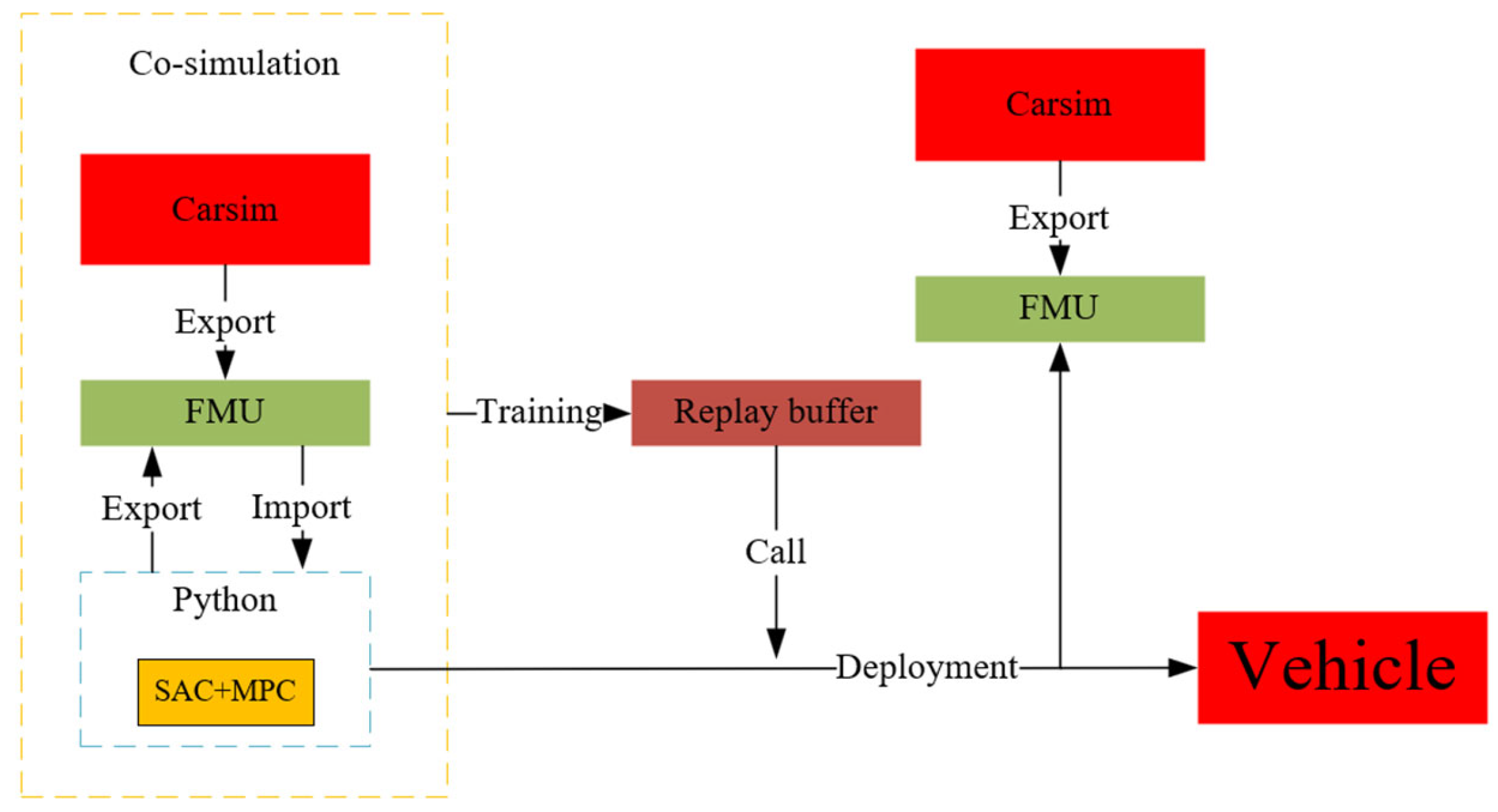
To validate the effectiveness of the SAC parameter-tuning MPC controller, simulations are conducted under both double-lane-change normal operating conditions and docking operating conditions. To facilitate subsequent experimental deployment and minimize variable discrepancies during the transition from simulation to real-world implementation, the complete controller is deployed within the Python environment. The co-simulation is collaboratively realized through Python 3.8 and CarSim 2020, with the overall control framework being shown in
Figure 3. Specifically, both the SAC agent and the MPC controller are implemented in Python, and co-simulation is conducted by invoking the Functional Mock-up Unit (FMU) module exported from CarSim, where the CarSim component serves as the controlled vehicle model. This architectural design not only ensures flexibility during the preliminary training phase but also provides a unified code framework for subsequent real-vehicle deployment, thereby achieving seamless migration following the “simulation-to-reality transfer” paradigm [
17].
The computing platform employed for model training and deployment was configured with an AMD Ryzen 7 6800H processor operating at a base frequency of 3.2 GHz (actual operating frequency: 3.17 GHz), a GeForce GTX 3060 graphics processing unit, and 16 GB of dual-channel memory (2 × 8 GB modules) with a data transfer rate of 4800 MT/s [
18].
The vehicle model is selected as the C-Class vehicle in CarSim, with specific parameters presented in
Table 2.
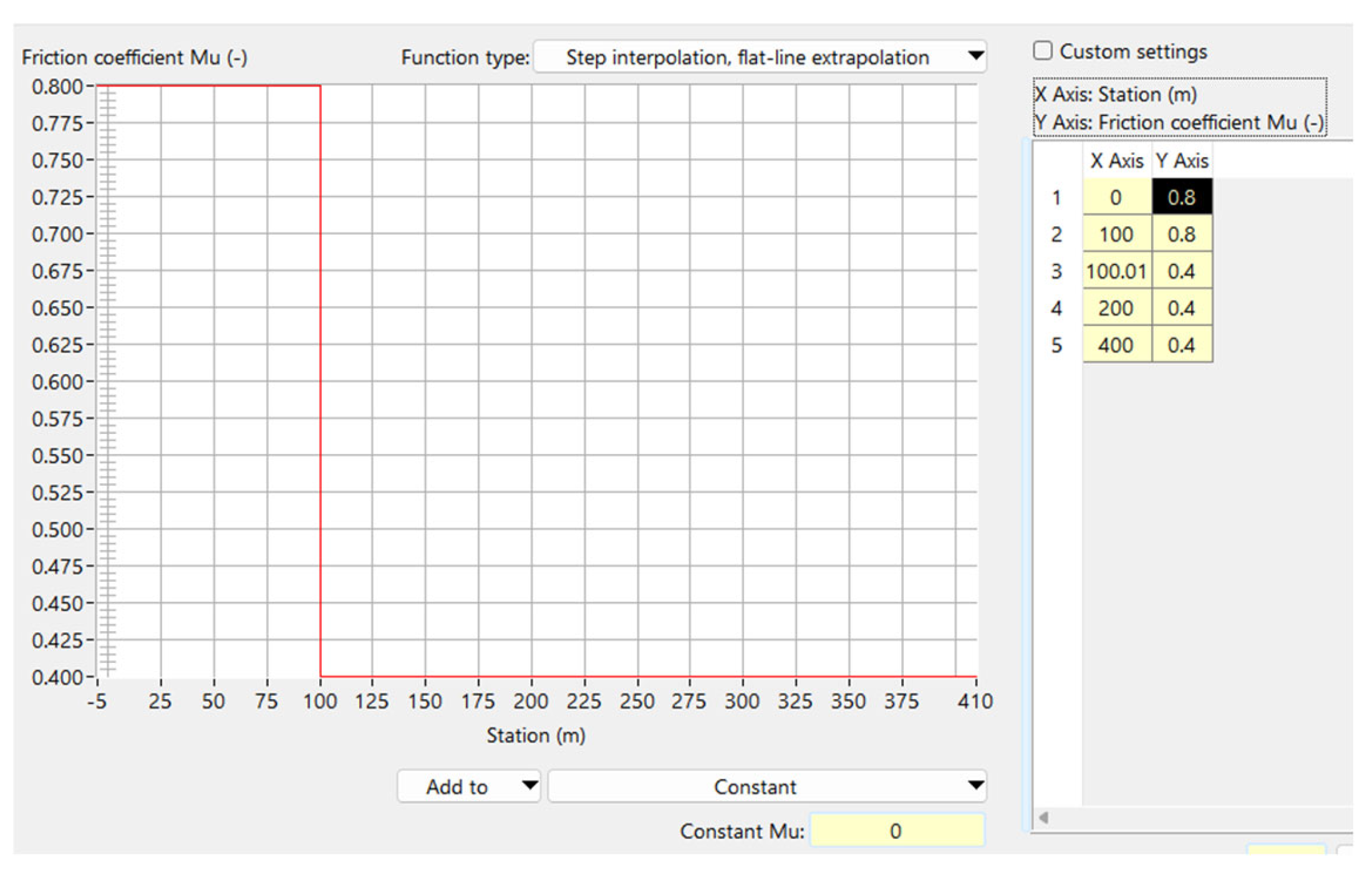
During the co-simulation with CarSim, the road surface adhesion coefficients for different segments can be configured within the CarSim road model.
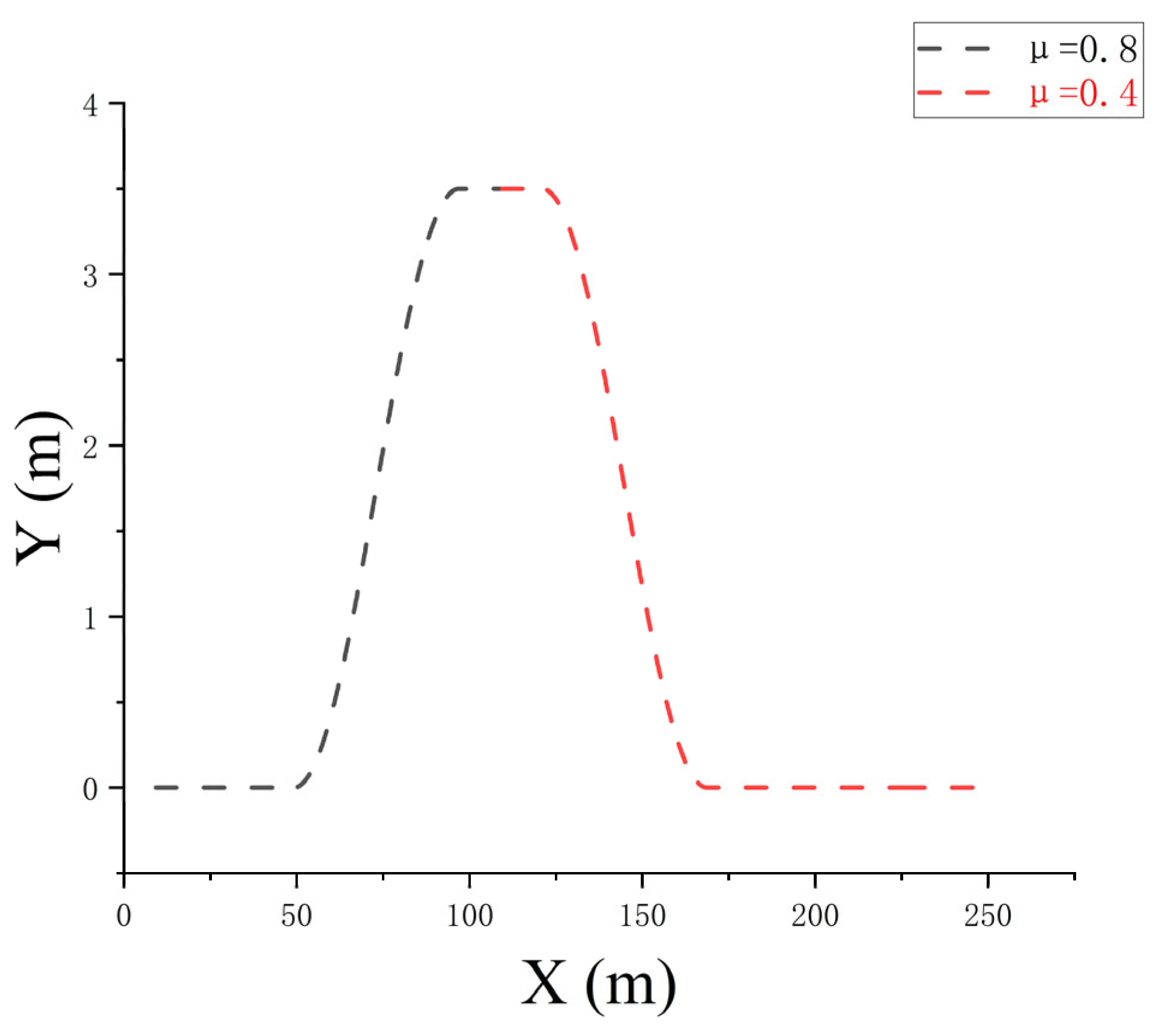
Figure 4 illustrates the road surface adhesion coefficient configuration scheme for the docking scenario, while the normal operating condition can be realized by simply adjusting the adhesion coefficient values. In real-vehicle experiments, the actual road surface adhesion coefficient can be obtained through straightforward friction coefficient traction tests.
It is noteworthy that the system exhibits robust performance when measurement errors exist in the intelligent vehicle’s detection of road surface adhesion coefficients. Specifically, if the actual road surface adhesion coefficient exceeds the detected value (conservative estimation), the control performance remains essentially unaffected. Conversely, if the actual adhesion coefficient falls below the detected value, although the control performance experiences slight degradation, the overall system performance remains stable. This characteristic fully demonstrates the adaptive advantages and robustness of the SAC algorithm.
5.1. Double-Lane-Change Normal Operating Condition
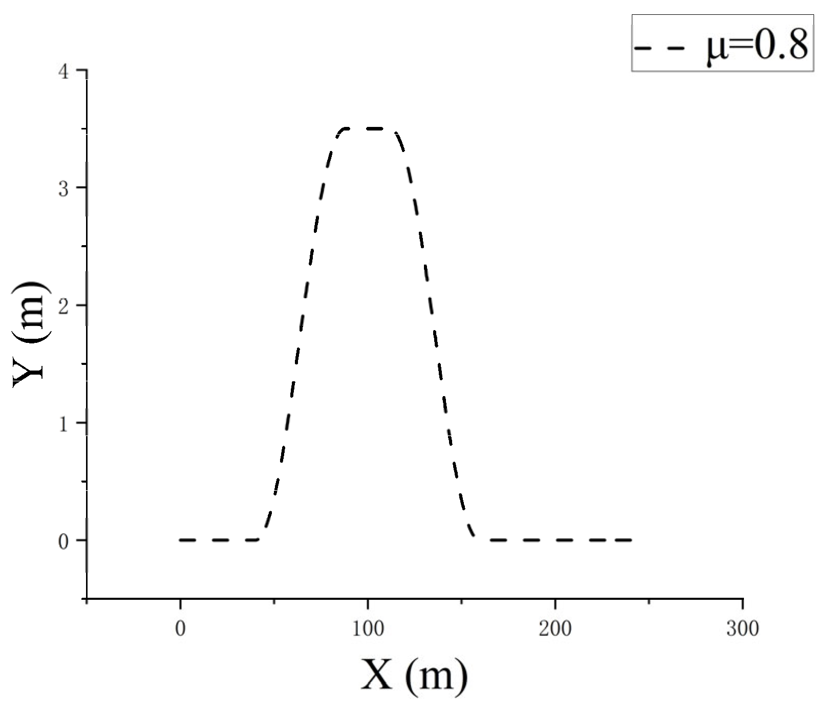
To verify the feasibility of the algorithm under normal operating conditions, a double-lane-change maneuver is first conducted. The vehicle speed is fixed at 60 km/h, the road surface adhesion coefficient is μ = 0.8 (constant), and the trajectory is illustrated in
Figure 5.
Figure 5 depicts the normal double-lane-change trajectory, and
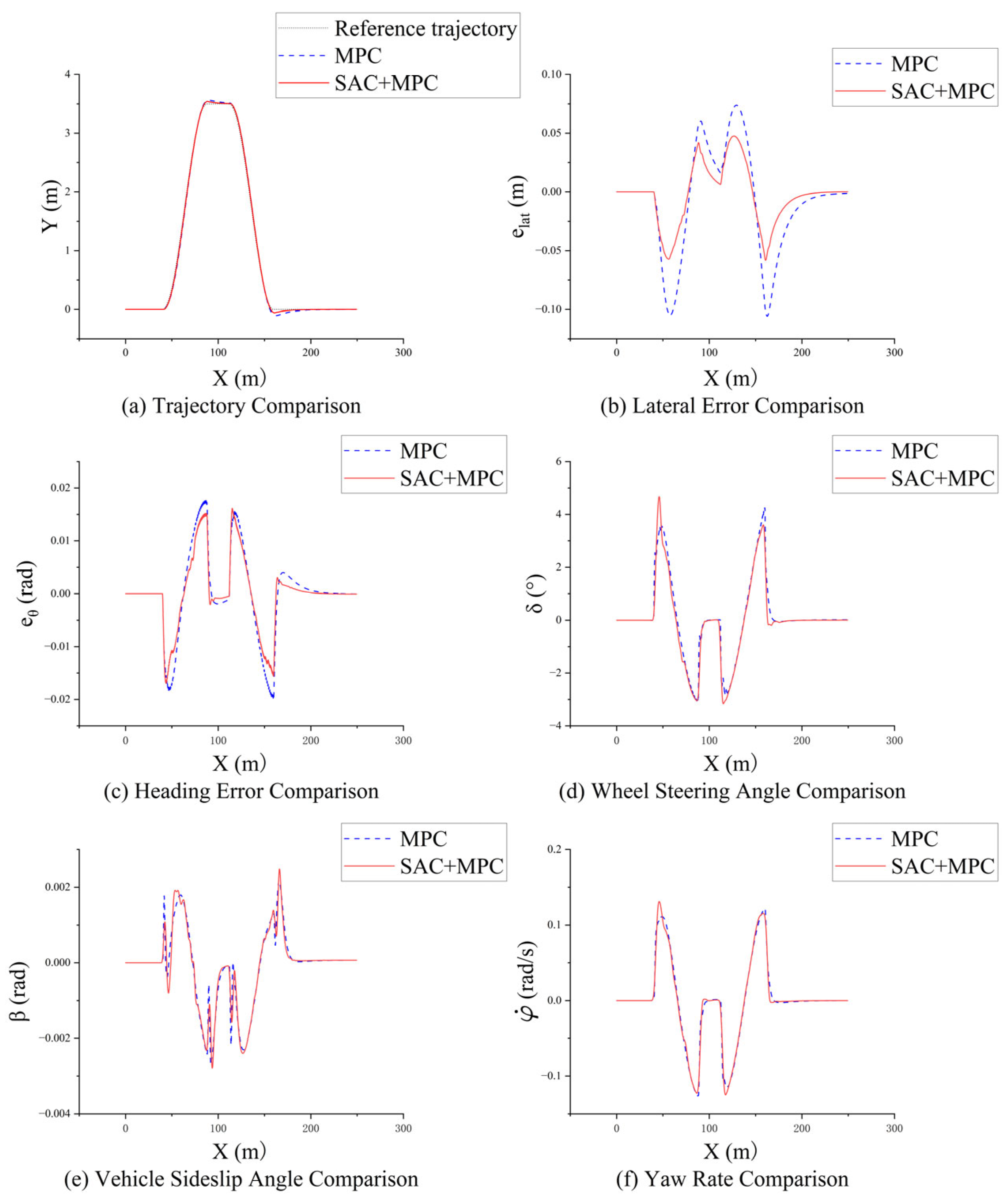
Figure 6 presents a comparison of path tracking between fixed-parameter MPC and SAC-MPC. The simulation results are shown in
Figure 6.
Figure 6a Comparison of tracking trajectories;
Figure 6b Comparison of lateral errors;
Figure 6c Comparison of heading errors;
Figure 6d Comparison of wheel steering angles;
Figure 6e Comparison of tire slip angles;
Figure 6f Comparison of yaw rates.
The simulation results reveal that in the trajectory tracking performance of the SAC-tuned integrated controller and the MPC-based controller, both controllers exhibit close conformity to the desired reference path, whereas the latter demonstrates comparatively larger deviations. A notable reduction in lateral displacement error can be observed from the comparative analysis. Additionally, the heading angle deviation is maintained at a lower magnitude throughout the maneuver. The dynamic responses, including steering wheel angle, vehicle sideslip angle at the mass center, and yaw rate, demonstrate superior consistency and alignment with the reference values under the proposed control strategy.
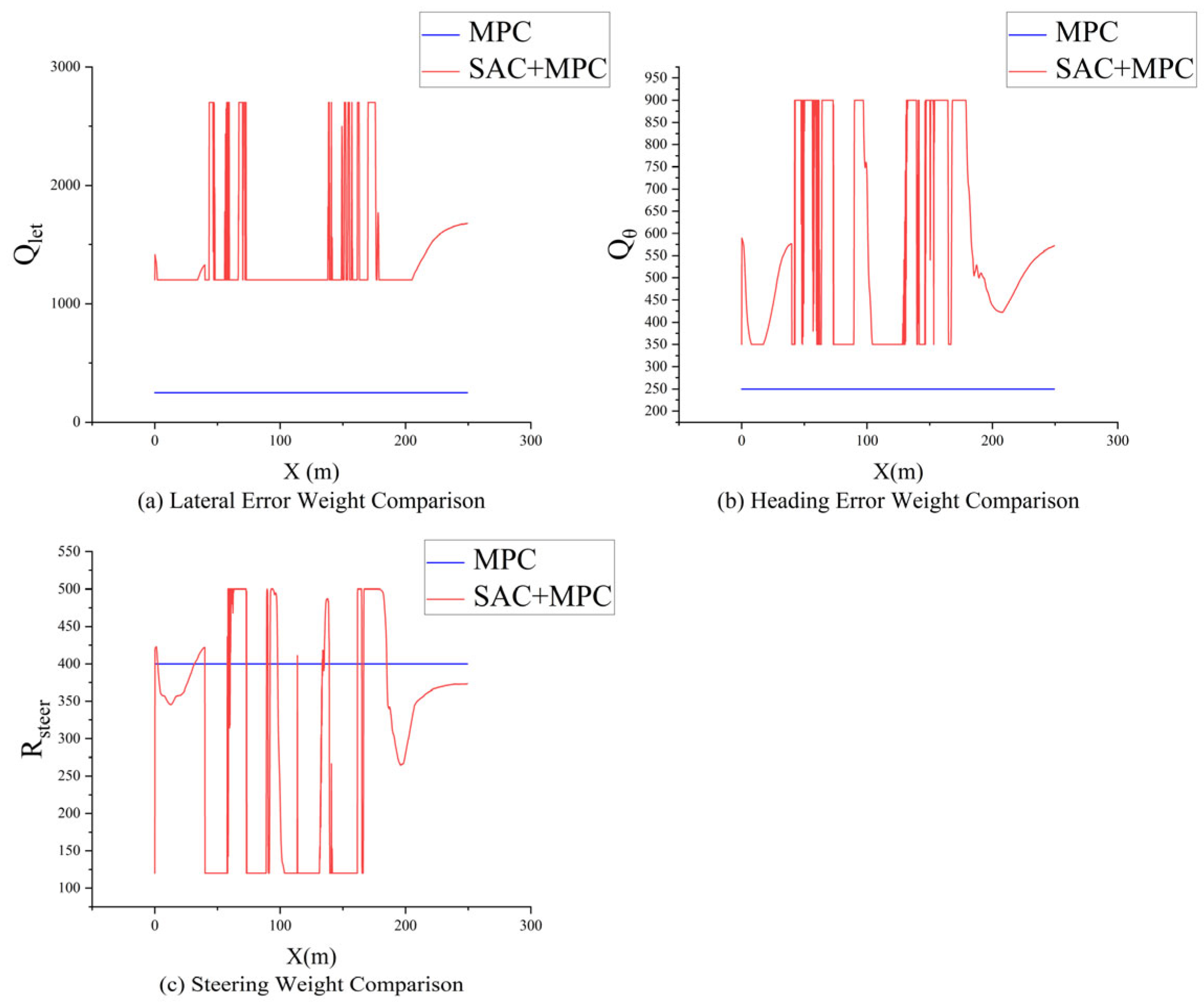
Figure 7 presents the parameter tuning comparison results for
,
, and
under the double-lane-change operating condition.
Figure 7a Lateral error weight map;
Figure 7b Heading error weight map;
Figure 7c Steering weight map. It can be observed that parameter tuning is not particularly pronounced during straight-line segments. During the lane change process, however, parameter tuning occurs frequently, with the weight for the heading error being particularly increased, and the weight for the lateral error also correspondingly being increased, thereby achieving higher tracking accuracy.
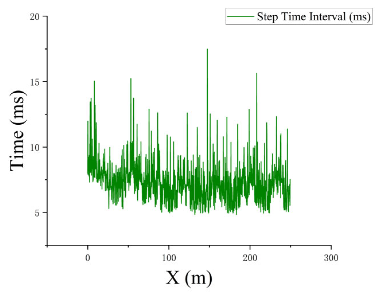
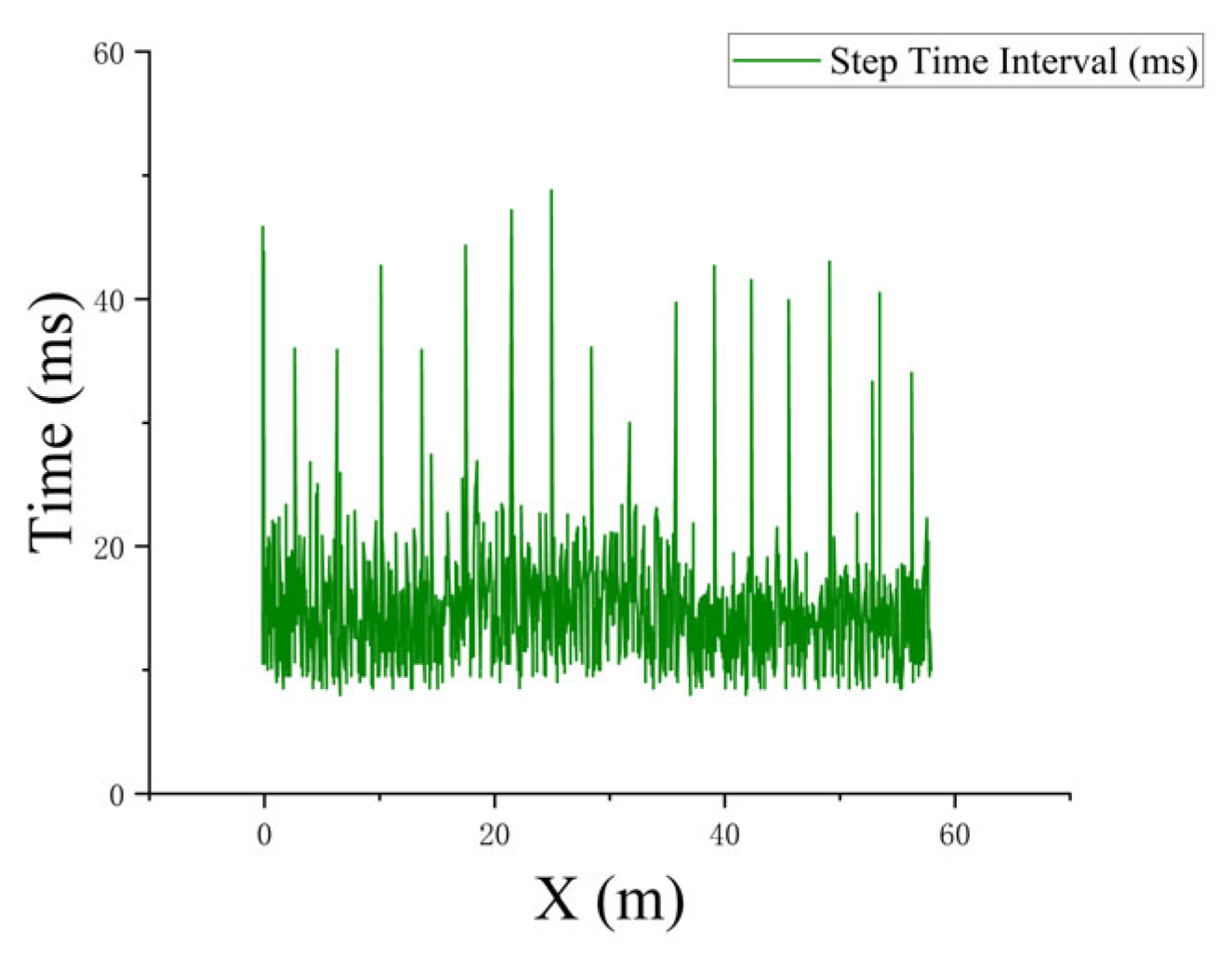
Figure 8 illustrates the execution time per step during the simulation process, while
Table 3 provides a detailed statistical analysis of the execution time. The simulation control frequency is configured at 50 Hz, corresponding to a single-step time budget of 20 ms. The analysis results indicate that the maximum single-step execution time in the simulation is 17.49 ms, which satisfies the real-time requirement (<20 ms). Although temporal variations in execution time are observed, all measured data points remain within the time constraint, with the average execution time remaining below 8 ms, representing a substantial safety margin. Consequently, the simulation scenario achieves stable real-time operation.
The quantitative data analysis of tracking accuracy and stability indicators from the specific simulation results is presented in
Table 4. As shown in
Table 4, compared with the conventional MPC-based path-tracking control, the reinforcement-learning-based tuning method reduces the maximum absolute lateral error and mean lateral error by 44.9% and 67.2%, respectively; the maximum absolute heading error is reduced by 23.5%; and smoother steering wheel angles are achieved.
Therefore, it can be concluded that the MPC with SAC-based parameter tuning demonstrates higher accuracy under normal double-lane-change path-tracking operating conditions.
5.2. Double-Lane-Change Docking Operating Condition
Having verified the feasibility of the algorithm under normal operating conditions, the transition operating condition is validated next. The vehicle speed is maintained at 60 km/h, and at x = 100 m, the road surface adhesion coefficient abruptly undergoes a transition from μ = 0.8 to μ = 0.4, thereby simulating a transition scenario from high-adhesion to low-adhesion road surfaces. The trajectory is illustrated in
Figure 9.
The simulation results are presented in
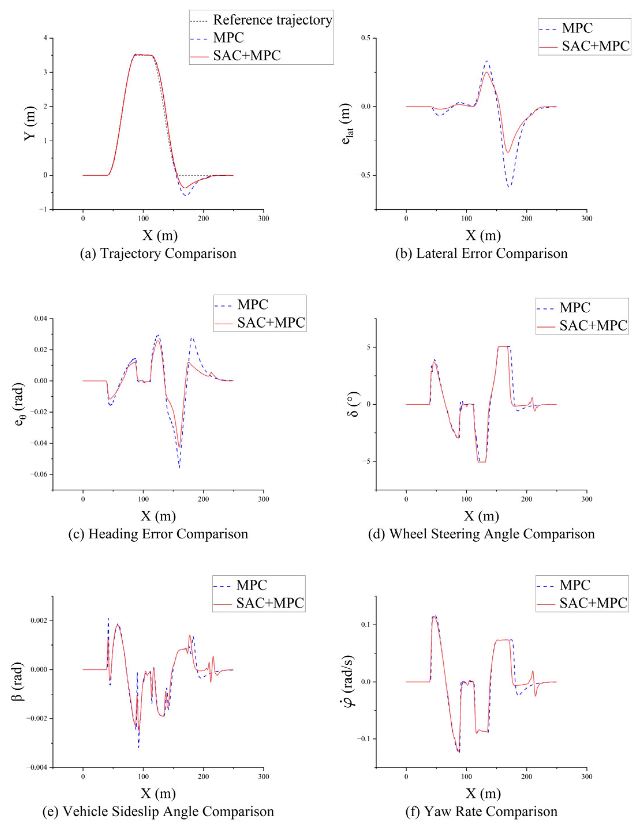
Figure 10. As shown in
Table 5, when the road surface adhesion coefficient changes abruptly, the maximum absolute lateral error of the fixed-parameter MPC reaches 0.59 m, indicating its poor adaptability to the docking operating conditions. In contrast, the maximum absolute lateral error of SAC-MPC is reduced to 0.334 m, representing a reduction of approximately 43.4%; the maximum absolute heading error is reduced by 23.8% compared with the fixed-parameter MPC. As illustrated in
Figure 10 and
Table 5,
Figure 10a Comparison of tracking trajectories;
Figure 10b Comparison of lateral errors;
Figure 10c Comparison of heading errors;
Figure 10d Comparison of wheel steering angles;
Figure 10e Comparison of tire slip angles;
Figure 10f Comparison of yaw rates. The maximum absolute yaw rates are comparable; however, the front wheel steering angle response of SAC-MPC is more advanced, demonstrating the advantage of the reinforcement learning strategy. Furthermore, the maximum absolute sideslip angle at the center of gravity is reduced by 20.7%, reflecting that SAC-MPC exhibits a stronger vehicle lateral stability and handling response under nonlinear operating conditions.
Figure 11 presents the parameter tuning comparison results for
,
, and
under the Double-Lane-Change docking operating condition.
Figure 11a Lateral error weight map;
Figure 11b Heading error weight map;
Figure 11c Steering weight map. It can be observed that parameter tuning is not particularly pronounced during straight-line segments. During the lane change process, however, parameter tuning occurs frequently, with the weight for the heading error being particularly increased, and the weight for the lateral error also correspondingly being increased, thereby achieving higher tracking accuracy.
Figure 12 illustrates the execution time per step during the simulation process, while
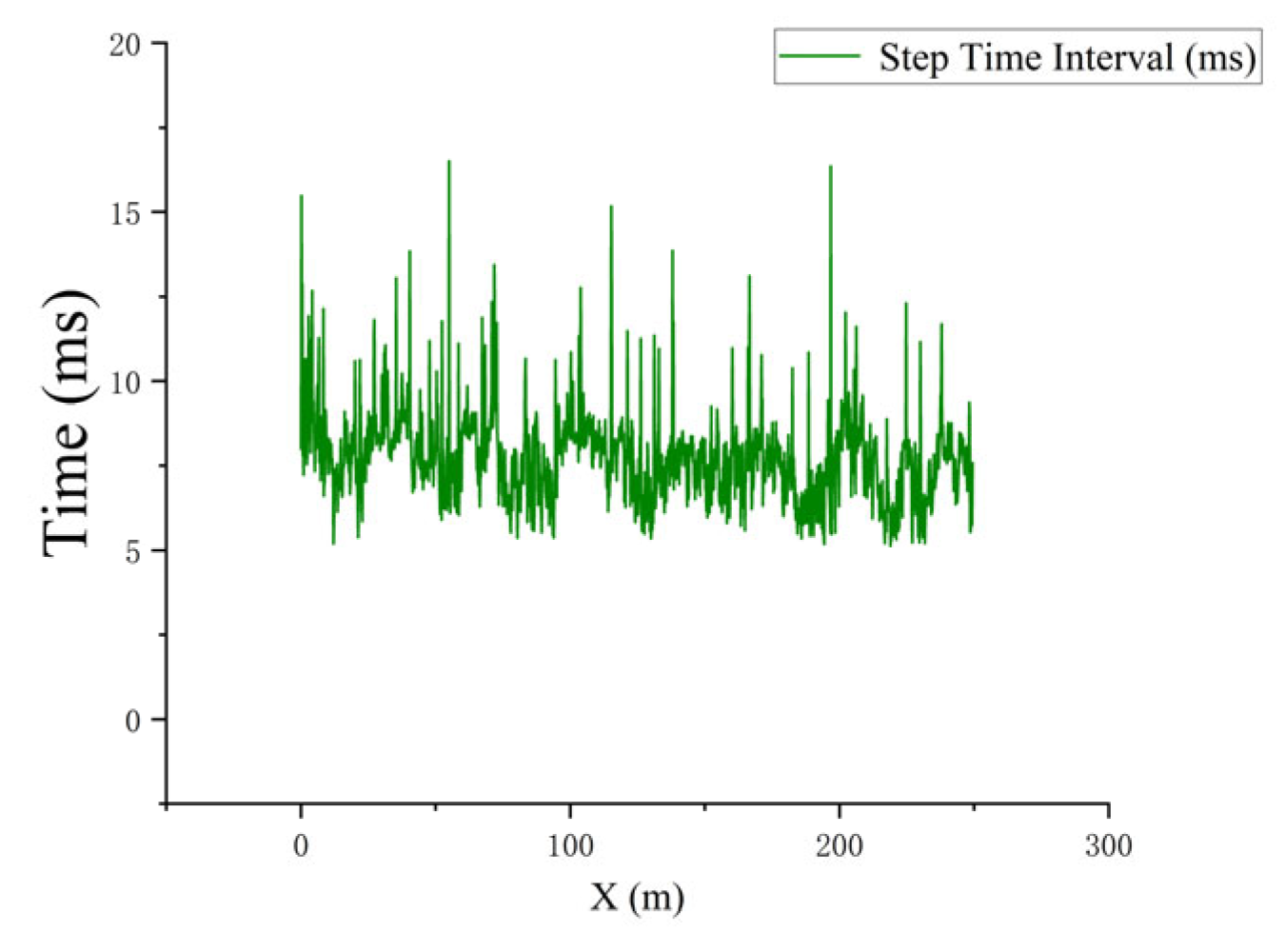
Table 6 provides a detailed statistical analysis of the execution time. The simulation control frequency is configured at 50 Hz, corresponding to a single-step time budget of 20 ms. The analytical results indicate that the maximum single-step execution time in the simulation is 16.5042 ms, which satisfies the real-time requirement (<20 ms). Although temporal variations in execution time are observed, all sampling points remain within the time constraint, with the average execution time maintained below 8 ms, representing a substantial safety margin. Consequently, the simulation scenario achieves stable real-time operation.
6. Experimental Validation
The experimental vehicle is a low-speed by-wire chassis featuring four-wheel independent steering, independent driving, and independent suspension based on in-wheel motor drives, which was developed by the research team. The specific vehicle parameters are presented in
Table 7.
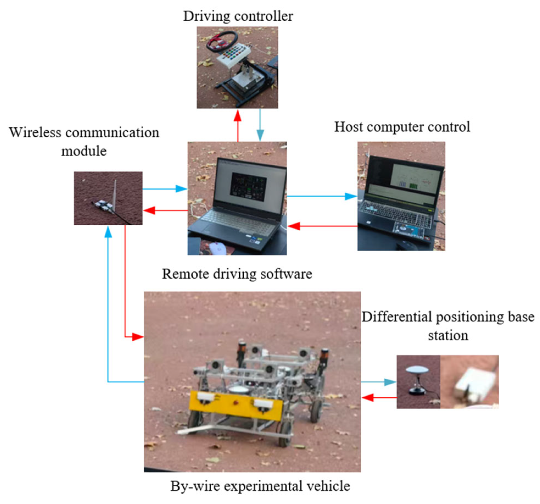
The wire-controlled experimental chassis system is illustrated in
Figure 13, which primarily comprises the driving controller, wire-controlled experimental chassis, remote driving software, and host computer. The host computer receives vehicle parameters and GNSS signals through UDP data packets for real-time processing. The processed information is then transmitted to the vehicle’s VCU via UDP data packets. Subsequently, the vehicle’s VCU sends commands to the driving controller and GNSS (Global Navigation Satellite System) to implement real-time closed-loop control.
The experimental platform is equipped with independent remote driving software, which can form a complete remote driving closed-loop system with the vehicle and hardware facilities in the absence of a host computer. The host computer communicates with the designated interface of the experimental platform’s remote driving system, solely through UDP packets for control purposes. Based on this architecture, the SAC algorithm is trained in the Python-CarSim co-simulation environment, with all reinforcement learning and control programs deployed in Python, while CarSim serves exclusively as the controlled plant. This design ensures high consistency between the simulation system and experimental validation approach. During the transition from simulation deployment to real-vehicle verification, only two substitutions are required: (1) replacing the controlled plant from the CarSim model to the experimental platform and (2) integrating the GNSS signal from the experimental system, thereby enabling rapid deployment of the complete experimental system. The co-simulation between Python and CarSim is realized through the FMU (Functional Mock-up Unit) interface, which exhibits minimal simulation latency and enables automatic episode transitions during training without manual intervention. Considering the substantial discrepancies between the CarSim standard vehicle model and the experimental platform, a vehicle dynamics model that is specifically tailored to match the characteristics of the experimental platform is developed for training purposes.
In this experimental system, the host computer is not involved in low-level control operations. The workflow proceeds as follows: the host computer transmits intelligent driving mode requests via UDP packets over the wireless communication module, simultaneously issuing throttle opening and steering wheel angle commands (both velocity and angle are regulated through PID closed-loop control); upon reception, the VCU forwards the information to the vehicle-driving controller through the wireless communication module; the controller then relays the information to the remote driving software; finally, the remote driving software transmits control commands to the VCU for low-level control execution. This hierarchical architecture ensures that the intelligent driving control system does not directly participate in low-level execution, maintaining driver operation priority over the intelligent driving system at all times, thereby guaranteeing safety.
Considering that excessively high control frequencies would exceed the hardware performance limits, the control frequency is configured at 50 Hz in this study. Meanwhile, data packet frequencies for non-control loops such as GNSS can be set higher. This implies that as long as the single-step computation time remains below 20 ms (1/50 s), the real-time control requirement is satisfied.
Due to the difficulty in achieving the experimental conditions for the docking operating condition, this experiment only conducts a double-lane-change path-tracking experiment for validation.
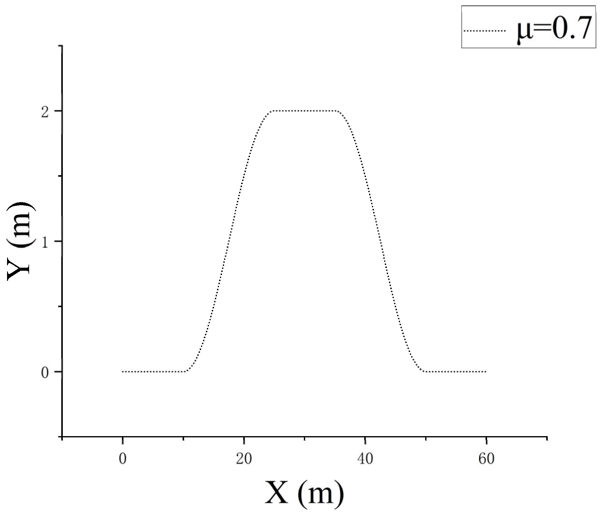
Considering the difficulty in implementing nonlinear operating conditions, and that the combined effects of various delays and vehicle manufacturing tolerances render the experiment approximately equivalent to nonlinear conditions, the double-lane-change (DLC) maneuver is temporarily adopted for experimental comparison. Given the significant dimensional differences between the drive-by-wire experimental chassis and full-scale vehicles, the DLC trajectory has been adjusted accordingly. In accordance with the (JTC D20-2006), and considering the constraints of the current experimental scenario, the standard double-lane-change maneuver was proportionally scaled. The experimental vehicle speed was set to 10.8 km/h, the road surface friction coefficient was 0.7, and the reference trajectory is shown in
Figure 14.
The trajectory diagram in
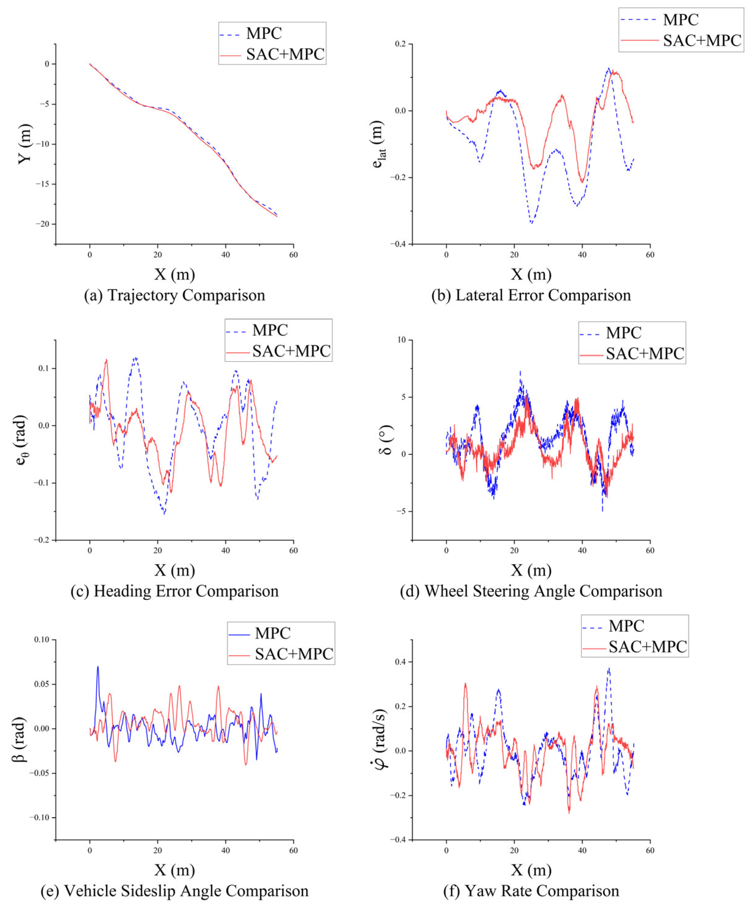
Figure 15a is presented in the north-east (NE) coordinate system of the experimental chassis. The simulation results are shown in
Figure 15.
Figure 15a Comparison of tracking trajectories;
Figure 15b Comparison of lateral errors;
Figure 15c Comparison of heading errors;
Figure 15d Comparison of wheel steering angles;
Figure 15e Comparison of tire slip angles;
Figure 15f Comparison of yaw rates. As indicated in
Table 8, the proposed SAC algorithm demonstrates significant improvements over the baseline controller, with the maximum absolute lateral error and mean absolute lateral error reduced by approximately 36.2% and 78.1%, respectively; the maximum absolute heading angle error is reduced by 24.3% compared to the fixed-parameter MPC; a reduction of 19.6% is achieved in the maximum absolute yaw rate; and the maximum absolute sideslip angle is reduced by 30.8%. However, the front wheel steering angle response of SAC-MPC is more conservative, demonstrating the advantage of the reinforcement learning strategy. Moreover, during the lane change process, the adjustment trend of the weighting coefficient for lane-change accuracy is consistently toward the maximum value. Therefore, this experiment validates that the MPC algorithm based on SAC parameter tuning exhibits superior performance.
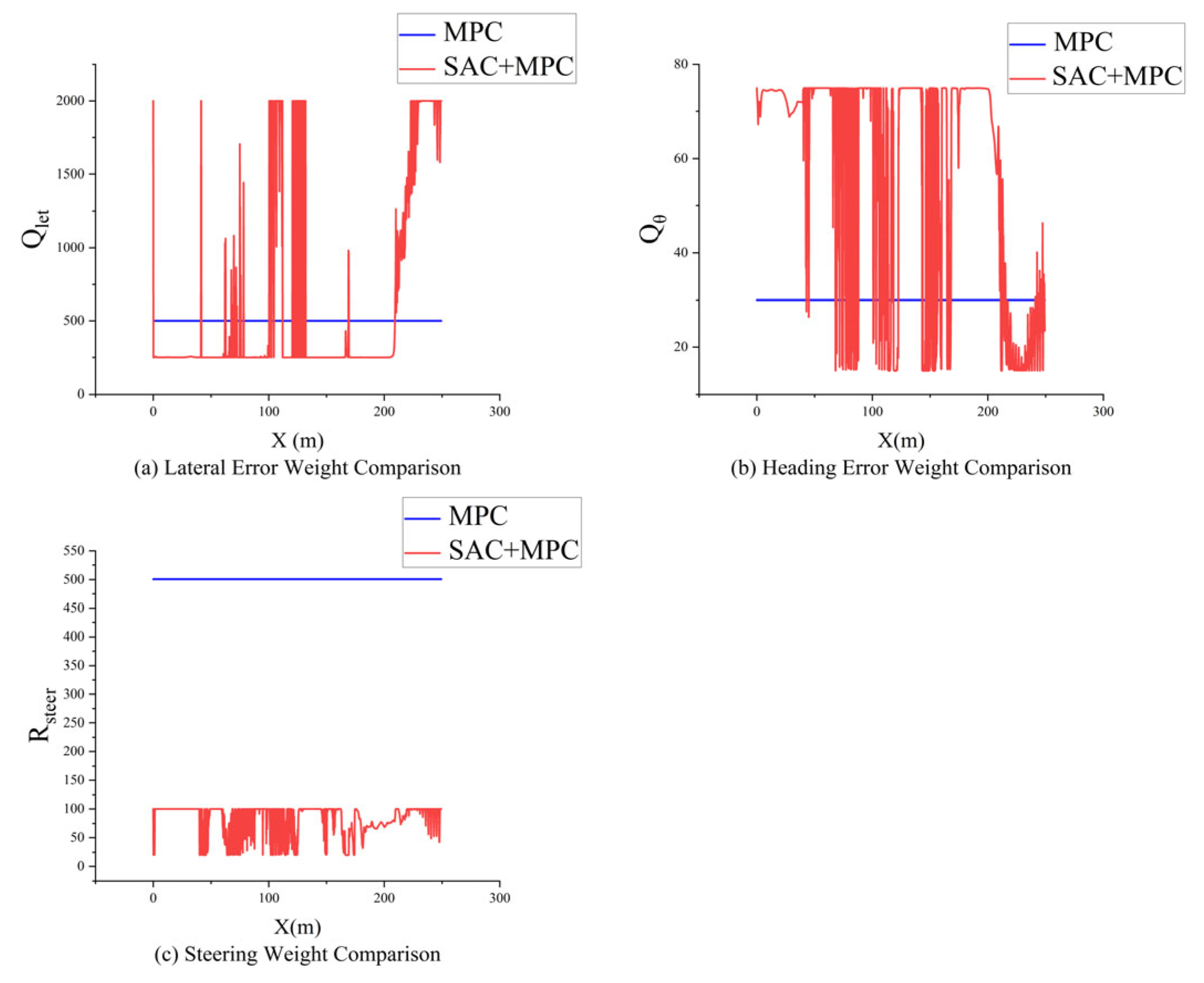
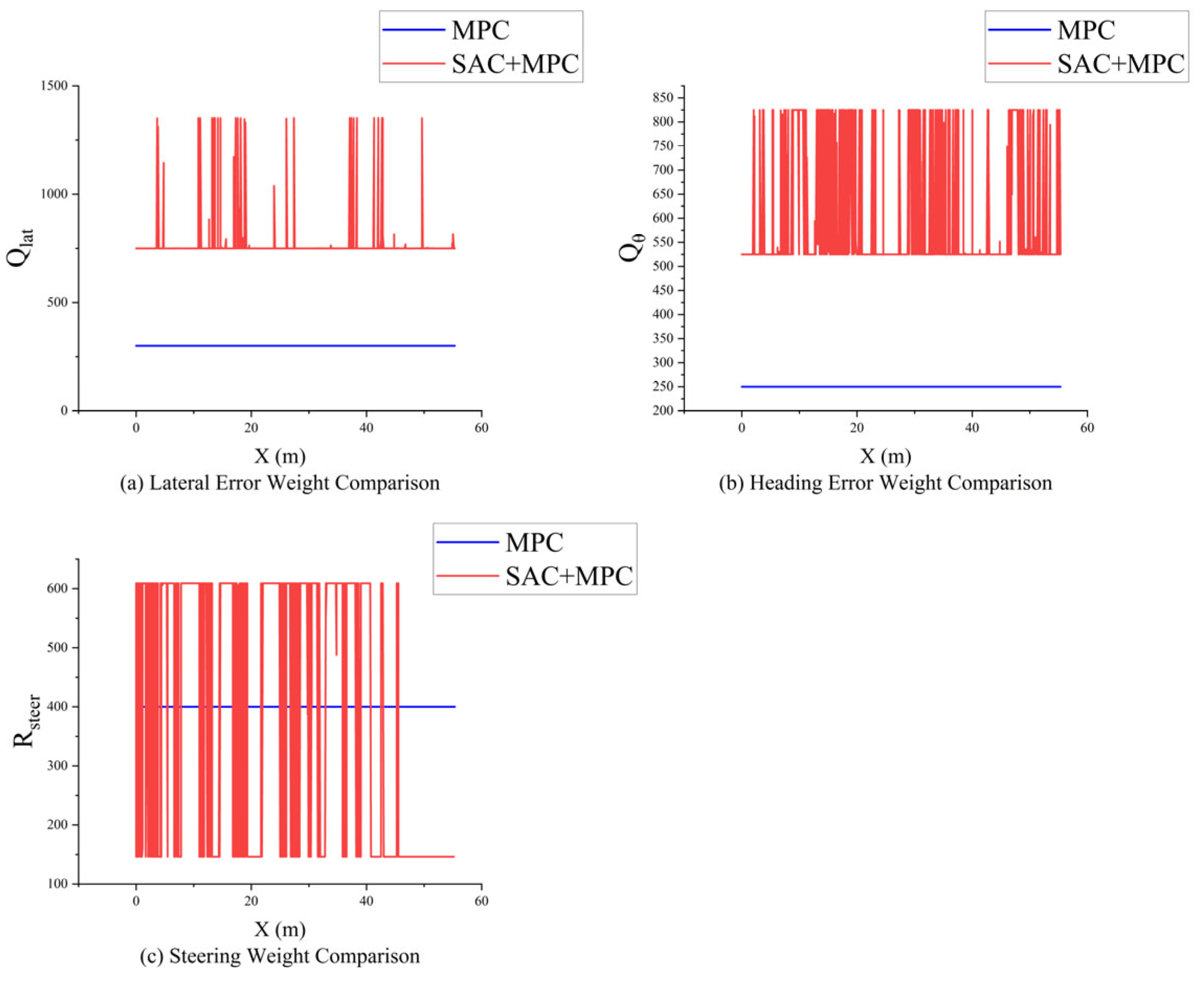
Figure 16 presents the parameter tuning comparison results for
,
, and
under the double-lane-change experiment.
Figure 16a Lateral error weight map;
Figure 16b Heading error weight map;
Figure 16c Steering weight map. It can be observed that parameter tuning is not particularly pronounced during straight-line segments. During the lane change process, however, parameter tuning occurs frequently, with the weight for the heading error being particularly increased, and the weight for the lateral error also correspondingly being increased, thereby achieving higher tracking accuracy.
Figure 17 illustrates the execution time per step during the experimental process, while
Table 9 provides a detailed statistical analysis of the execution time. Considering the actual hardware performance of the experimental vehicle, the control frequency is configured at 20 Hz, corresponding to a single-step time budget of 50 ms. The analytical results indicate that the maximum single-step execution time is 48.79212 ms, which satisfies the real-time requirement (<50 ms). Although temporal variations in execution time are observed, all sampling points remain within the time constraint, with the average execution time maintained below 15 ms, representing a substantial safety margin. Consequently, the experimental system achieves stable real-time operation.
7. Conclusions
To address the challenges of tracking accuracy degradation and stability deterioration faced by intelligent vehicles under various operating conditions, this paper proposes a variable-parameter Model Predictive Control (MPC) multi-objective strategy based on SAC reinforcement learning to achieve adaptive control of intelligent vehicle path tracking. Through simulation and actual vehicle experimental validation, the following conclusions are drawn.
The MPC controller with parameter tuning accomplished through SAC reinforcement learning demonstrates superior performance compared to the fixed-parameter MPC scheme and exhibits stronger adaptability to different operating conditions. It can achieve an adaptive trade-off between tracking accuracy and stability under various operating conditions. According to the simulation results, under normal operating conditions, the integrated control based on SAC and MPC demonstrates superior tracking accuracy. Under nonlinear operating conditions, the integrated control based on SAC and MPC shows significant improvements in both the tracking accuracy and stability during docking conditions. Corresponding experiments have been conducted for validation, confirming the conclusions derived from simulations.
The SAC reinforcement-learning parameter-tuning method proposed in this paper demonstrates favorable performance in handling continuous control problems and can autonomously explore and generate optimal strategies. However, comparative studies on the training time consumption and generalization capability of this method still require further investigation.
Based on the soft actor-critic (SAC) reinforcement learning framework, the Model Predictive Control (MPC) controller with parameter tuning demonstrates superior control performance compared to the fixed-parameter MPC method, with significantly enhanced adaptability across various operating conditions. This approach enables improved path-tracking accuracy under multiple operating scenarios. The simulation results indicate that under conventional operating conditions, the integrated control strategy combining SAC and MPC exhibits superior tracking precision, with the maximum absolute value and mean value of the lateral error reduced by 44.9% and 67.2%, respectively, and the maximum absolute value of the heading angle error reduced by 23.5%. Under nonlinear operating conditions, the SAC-MPC integrated control achieves significant improvements in both tracking accuracy and control stability during condition transitions. The analysis of simulation results reveals that, compared to fixed-parameter MPC, the SAC-based parameter-tuning MPC method reduces the maximum absolute value of the lateral error by approximately 43.4%, the maximum absolute value of heading angle error by 23.8%, and the sideslip angle at the center of gravity by 20.7%, demonstrating that reinforcement-learning-based parameter tuning can effectively enhance vehicle lateral stability and handle response characteristics under nonlinear operating conditions. Corresponding experimental validation was conducted in this study. The analysis of the experimental results demonstrates that, compared to fixed-parameter MPC, this method reduces the maximum absolute value and mean value of the lateral error by approximately 36.2% and 78.1%, respectively; the maximum absolute value of the heading angle error by 24.3%; the maximum absolute value of the yaw rate by 19.6%; and the maximum absolute value of the sideslip angle at the center of gravity by 30.8%, thereby validating the effectiveness of the conclusions obtained from simulations.
In summary, the SAC reinforcement-learning-based parameter-tuning method proposed in this paper exhibits favorable performance in addressing continuous control problems and is capable of autonomously exploring and generating optimal control strategies. However, comparative investigations of the generalization performance of the proposed method against other state-of-the-art reinforcement learning algorithms remain to be carried out. Moreover, the hardware architecture for experimental setups and the construction of diverse multi-condition operating scenarios still require further optimization in future work.
Author Contributions
Conceptualization, J.Z. and Z.L.; methodology, J.Z. and Z.L.; software, J.Z.; validation, J.Z., Z.L., X.Y., Y.T. and H.Z.; formal analysis, J.Z., Y.T. and Z.L.; investigation, J.Z., X.Y.; resources, Z.L., X.Y., J.Z. and H.Z.; data curation, J.Z.; writing—original draft preparation, J.Z.; writing—review and editing, J.Z.; visualization, J.Z.; supervision, H.Z. and Y.T.; project administration, J.Z., X.Y. and J.Z.; funding acquisition, Z.L., X.Y. All authors have read and agreed to the published version of the manuscript.
Funding
This research is supported by the Science and Technology Innovation Talents Support Program of Henan Provincial Universities (grant no. 25HASTIT037).
Data Availability Statement
The original contributions presented in this study are included in the article. Further inquiries can be directed to the corresponding author.
Conflicts of Interest
The authors declare no conflicts of interest.
References
- Li, C.; Jiang, H.; Yang, X.; Wei, Q. Path Tracking Control Strategy Based on Adaptive MPC for Intelligent Vehicles. Appl. Sci. 2025, 15, 5464. [Google Scholar] [CrossRef] [Scilit]
- Domina, Á.; Tihanyi, V. LTV-MPC Approach for Automated Vehicle Path Following at the Limit of Handling. Sensors 2022, 22, 5807. [Google Scholar] [CrossRef] [Scilit] [PubMed]
- He, J.; Su, S.; Wang, H.; Chen, F.; Yin, B. Online PID Tuning Strategy for Hydraulic Servo Control Systems via SAC-Based Deep Reinforcement Learning. Machines 2023, 11, 593. [Google Scholar] [CrossRef] [Scilit]
- Kabzan, J.; Hewing, L.; Liniger, A.; Zeilinger, M.N. Learning-Based Model Predictive Control for Autonomous Racing. IEEE Robot. Autom. Lett. 2019, 4, 3363–3370. [Google Scholar] [CrossRef] [Scilit]
- Wang, H.; Wang, C.; Zhao, L.; Hu, Y. Variable-Parameter MPC Multi-Objective Control for Intelligent Vehicle Path Tracking Based on Reinforcement Learning. China J. Highw. Transp. 2024, 37, 157–169. [Google Scholar] [CrossRef]
- Wang, H.; Liu, B.; Ping, X.; An, Q. Path Tracking Control for Autonomous Vehicles Based on an Improved MPC. IEEE Access 2019, 7, 161064–161073. [Google Scholar] [CrossRef] [Scilit]
- Jin, H.; Lu, K. Intelligent Vehicle Trajectory Tracking Based on Multi-Parameter Adaptive Optimization. China J. Highw. Transp. 2023, 36, 260–272. [Google Scholar] [CrossRef]
- Wang, H.; Wang, Q.; Chen, W.; Zhao, L.; Tan, D. Path Tracking Based on Model Predictive Control with Variable Predictive Horizon. Trans. Inst. Meas. Control 2021, 43, 2676–2688. [Google Scholar] [CrossRef] [Scilit]
- Mnih, V.; Kavukcuoglu, K.; Silver, D.; Graves, A.; Antonoglou, I.; Wierstra, D.; Riedmiller, M. Playing Atari with Deep Reinforcement Learning. arXiv 2013, arXiv:1312.5602. [Google Scholar] [CrossRef] [Scilit]
- Lillicrap, T.P.; Hunt, J.J.; Pritzel, A.; Heess, N.; Erez, T.; Tassa, Y.; Silver, D.; Wierstra, D. Continuous Control with Deep Reinforcement Learning. arXiv 2019, arXiv:1509.02971. [Google Scholar] [CrossRef] [Scilit] [PubMed]
- Fujimoto, S.; van Hoof, H.; Meger, D. Addressing Function Approximation Error in Actor-Critic Methods. In Proceedings of the 35th International Conference on Machine Learning; PMLR: New York, NY, USA, 2018. [Google Scholar]
- Haarnoja, T.; Zhou, A.; Abbeel, P.; Levine, S. Soft Actor-Critic: Off-Policy Maximum Entropy Deep Reinforcement Learning with a Stochastic Actor. arXiv 2018. [Google Scholar] [CrossRef] [Scilit]
- Liang, Z.; Zhang, H.; Zhao, J.; Wang, Y. Trajectory Tracking Control of Unmanned Vehicles Based on Adaptive MPC. J. Northeast. Univ. Sci. 2020, 41, 835–841. [Google Scholar] [CrossRef]
- Wang, Y.; Cai, Y.; Chen, L.; Wang, H.; He, Y.; Li, J. Design of Intelligent and Connected Vehicle Path Tracking Controller Based on Model Predictive Control. J. Mech. Eng. 2019, 55, 136–144+153. [Google Scholar] [CrossRef] [Scilit]
- Khlifi, A.; Othmani, M.; Kherallah, M. A Novel Approach to Autonomous Driving Using Double Deep Q-Network-Bsed Deep Reinforcement Learning. World Electr. Veh. J. 2025, 16, 138. [Google Scholar] [CrossRef] [Scilit]
- Li, T.; Cui, W.; Cui, N. Soft Actor-Critic Algorithm-Based Energy Management Strategy for Plug-In Hybrid Electric Vehicle. World Electr. Veh. J. 2022, 13, 193. [Google Scholar] [CrossRef] [Scilit]
- Qin, P.; Wu, F.; Bin, S.; Li, X.; Ya, F. High-Accuracy, High-Efficiency, and Comfortable Car-Following Strategy Based on TD3 for Wide-to-Narrow Road Sections. World Electr. Veh. J. 2023, 14, 244. [Google Scholar] [CrossRef] [Scilit]
- Han, B.; Sun, J. Road-Adaptive Precise Path Tracking Based on Reinforcement Learning Method. Sensors 2025, 25, 4533. [Google Scholar] [CrossRef] [Scilit] [PubMed]
Figure 1.
Flowchart of SAC algorithm.
Figure 1.
Flowchart of SAC algorithm.
Figure 2.
Reward function training curve.
Figure 2.
Reward function training curve.
Figure 3.
Control system framework flowchart.
Figure 3.
Control system framework flowchart.
Figure 4.
Friction coefficient settings in CarSim.
Figure 4.
Friction coefficient settings in CarSim.
Figure 5.
Normal double-lane-change trajectory.
Figure 5.
Normal double-lane-change trajectory.
Figure 6.
Comparison under standard double-lane-change maneuver.
Figure 6.
Comparison under standard double-lane-change maneuver.
Figure 7.
Comparison of weighting coefficients under normal double-lane-change operating condition.
Figure 7.
Comparison of weighting coefficients under normal double-lane-change operating condition.
Figure 8.
Operation time under normal working conditions.
Figure 8.
Operation time under normal working conditions.
Figure 9.
Connected double-lane-change trajectory.
Figure 9.
Connected double-lane-change trajectory.
Figure 10.
Data Comparison and Analysis of Double-Lane-Change Docking Operating Condition.
Figure 10.
Data Comparison and Analysis of Double-Lane-Change Docking Operating Condition.
Figure 11.
Comparison of weighting coefficients under docking double-lane-change operating condition.
Figure 11.
Comparison of weighting coefficients under docking double-lane-change operating condition.
Figure 12.
Operation time under docking double-lane-change working conditions.
Figure 12.
Operation time under docking double-lane-change working conditions.
Figure 13.
The wire-controlled experimental chassis system.
Figure 13.
The wire-controlled experimental chassis system.
Figure 14.
Experimental operating condition trajectory.
Figure 14.
Experimental operating condition trajectory.
Figure 15.
Comparison of double-lane-change experiment.
Figure 15.
Comparison of double-lane-change experiment.
Figure 16.
Experimental Condition Weight Comparison.
Figure 16.
Experimental Condition Weight Comparison.
Figure 17.
Operation time under experimental working conditions.
Figure 17.
Operation time under experimental working conditions.
Table 1.
Hyperparameter settings.
Table 1.
Hyperparameter settings.
| Indicator | Value |
|---|
| Actor Learning Rate | 0.0001 |
| Critic Learning Rate | 0.0001 |
| Smoothing Factor | 0.005 |
| Update Interval | 1 |
| Experience Replay Buffer | 100,000 |
| Discount Factor | 0.99 |
| Sampling Time | 0.01 |
Table 2.
Vehicle parameters.
Table 2.
Vehicle parameters.
| Vehicle Parameters | Value |
|---|
| Mass (kg) | 1660 |
| Front axles (m) | 1.2 |
| Rear axles (m) | 1.65 |
| Moment of inertia () | 1537 |
| Wheelbase (m) | 2.85 |
Table 3.
Double Lane Change Condition Runtime Analysis.
Table 3.
Double Lane Change Condition Runtime Analysis.
| Indicator | Time |
|---|
| Mean Execution Time (ms) | 7.2789 |
| Maximum Execution Time (ms) | 17.4866 |
| Minimum Execution Time (ms) | 4.8402 |
Table 4.
Comparison of tracking accuracy and stability under double-lane-change operating condition.
Table 4.
Comparison of tracking accuracy and stability under double-lane-change operating condition.
| Indicator | MPC | SAC-MPC |
|---|
| Maximum Absolute Lateral Error (m) | 0.10581 | 0.05825 |
| Mean Lateral Error (m) | 0.00816 | 0.00268 |
| Maximum Absolute Heading Error (rad) | 0.01987 | 0.0152 |
| Maximum Absolute Yaw Rate (rad/s) | 0.12625 | 0.13113 |
| Maximum Absolute Sideslip Angle (rad) | 0.00271 | 0.00279 |
Table 5.
Comparison of accuracy and stability under double-lane-change docking operating condition.
Table 5.
Comparison of accuracy and stability under double-lane-change docking operating condition.
| Indicator | MPC | SAC-MPC |
|---|
| Maximum Absolute Lateral Error (m) | 0.59016 | 0.33396 |
| Mean Lateral Error (m) | −0.04237 | −0.01661 |
| Maximum Absolute Heading Error (rad) | 0.05581 | 0.04253 |
| Maximum Absolute Yaw Rate (rad/s) | 0.12625 | 0.12184 |
| Maximum Absolute Sideslip Angle (rad) | 0.00319 | 0.00253 |
Table 6.
Docking Condition Runtime Analysis.
Table 6.
Docking Condition Runtime Analysis.
| Indicator | Time |
|---|
| Mean Execution Time (ms) | 7.73599 |
| Maximum Execution Time (ms) | 16.5042 |
| Minimum Execution Time (ms) | 5.1237 |
Table 7.
Parameters of wire-controlled experimental chassis.
Table 7.
Parameters of wire-controlled experimental chassis.
| Vehicle Parameters | Value |
|---|
| Mass (kg) | 60 |
| Front axles (m) | 0.45 |
| Rear axles (m) | 0.45 |
| Moment of inertia () | 24.3 |
| Wheelbase (m) | 0.9 |
Table 8.
Comparison of accuracy and stability under double-lane-change experimental operating condition.
Table 8.
Comparison of accuracy and stability under double-lane-change experimental operating condition.
| Indicator | MPC | SAC-MPC |
|---|
| Maximum Absolute Lateral Error (m) | 0.33838 | 0.21574 |
| Mean Lateral Error (m) | −0.10114 | −0.0222 |
| Maximum Absolute Heading Error (rad) | 0.15501 | 0.11739 |
| Maximum Absolute Yaw Rate (rad/s) | 0.38013 | 0.30561 |
| Maximum Absolute Sideslip Angle (rad) | 0.07034 | 0.04871 |
Table 9.
Experimental Condition Runtime Comparison.
Table 9.
Experimental Condition Runtime Comparison.
| Indicator | Time |
|---|
| Mean Execution Time (ms) | 14.40449 |
| Maximum Execution Time (ms) | 48.79212 |
| Minimum Execution Time (ms) | 8.00467 |
| Disclaimer/Publisher’s Note: The statements, opinions and data contained in all publications are solely those of the individual author(s) and contributor(s) and not of MDPI and/or the editor(s). MDPI and/or the editor(s) disclaim responsibility for any injury to people or property resulting from any ideas, methods, instructions or products referred to in the content. |
© 2026 by the authors. Published by MDPI on behalf of the World Electric Vehicle Association. Licensee MDPI, Basel, Switzerland. This article is an open access article distributed under the terms and conditions of the Creative Commons Attribution (CC BY) license.