Adaptive Large Neighborhood Search for a Flexible Truck–Drone Routing Problem with Multi-Visit and Cost Trade-Offs

Abstract

Extending the truck–drone mothership system, this paper addresses a flexible multi-visit truck and drone joint routing problem (FMTDJRP). A mixed integer linear program is proposed to minimize total travel cost. An adaptive large neighborhood search with a knowledge-based acceleration strategy yields near-optimal solutions. Experiments across varied customer distributions, drone specs, and truck-–drone cost ratios confirm flexibility, adaptability, and cost efficiency.

1. Introduction

A decade after Amazon’s eye-catching announcement on its plan about the use of drones for small parcel delivery [1], drone technology for delivery has been put into practice by many enterprises. By June 2022, Meituan drones have covered 10 communities and served 20,000 households in Shenzhen, China. With the completion of 100,000 deliveries in 2021, Google owns the largest residential drone delivery service in the world so far [2,3]. In the transportation and logistics field, unmanned and automated technologies are becoming a growing trend [4,5,6,7]. Even the global pandemic of COVID-19 has boosted the development in drone delivery [8]. Two main reasons can explain the enterprises’ embracement of drone technology for logistics.

First, drones can provide delivery services with significantly lower energy consumption and higher delivery speed. According to the study by Rodrigues [9], each package delivered by drones may consume up to 94% less energy compared with conventional transportation modes. Moreover, drones are less affected by road traffic conditions, enabling enterprises to gain a competitive advantage in delivery timeliness. At the same time, shifting part of the traffic flow to the air can help alleviate urban road congestion.

Second, reducing last-mile delivery costs remains a critical challenge in logistics. This stage can account for over 53% of the total transportation cost due to low average speeds, frequent parking-related energy consumption, and increased out-of-route distances [10]. Equipped with battery-powered propulsion systems and pre-planned flight paths, drones can effectively mitigate these inefficiencies and enhance the overall cost-effectiveness of last-mile delivery operations.

However, drones are currently not capable of long-distance and heavy-load trips due to regulatory rules and technological limitations. Therefore, truck–drone joint delivery becomes the best compromise. The pioneering research in this problem was made by Murray [11]. They described the truck–drone synchronization as a Flying Sidekick System (FSS) where a single drone is loaded on a truck and flies to serve customers when necessary. Another prominent synchronization pattern is the mothership system (MS), first studied by Karak [12]. Multiple drones are mounted on a truck and transported to places near customers so that they can take off to serve these customers. This system plays out advantages of drone fleets in terms of multiple customers being served in parallel.

In spite of the high efficiency brought by the application of drones, the conventional vehicles could be more efficient or even compulsory for a delivery in some cases [13]. From the technological aspect, some customers are located in such remote areas that they are not accessible by drones or their demands exceed the load capacity of drones. For these customers, only trucks can provide delivery service to them. From the ecological aspect, less C$O_2$ will be emitted if drones serve nearby customers and trucks serve ones farther away [14]. With the consideration of these factors, a flexible multi-visit truck and drone joint routing problem (FMTDJRP) is studied in this paper.

The FMTDJRP divides customers into large-demand ones and small-demand ones. Large-demand customers can only be visited by the truck because their demand exceeds the load capacity of drones, while small-demand customers can be served either by the truck or by drones. As a mothership system problem, satellites (facilities where trucks stop and drones are launched and retrieved) exist in the configuration of the FMTDJRP. Furthermore, drones are also allowed to take off and land at large-demand customers in the hope that the truck waiting time is made good use of when heavy goods are unloaded. These characteristics are where the flexibility comes from and what sets the problem apart from other mothership system problems.

Complexity comes along with the flexibility as well. First, the truck route and the drone routes are highly interdependent since small-demand customers can be in either of them. A small-demand customer removed from a drone route and inserted into the truck route results in changes to the sequences of nodes visited for both routes. Thus, separate optimization for the routes of two vehicles could lead to a sub-optimal solution.

Second, all nodes in the network of the FMTDJRP are not must-visit. Since the drone launch/retrieve operation is allowed at large-demand customers, there is a potential competitive relation between them and satellites to some extent. For instance, if a large-demand customer and a satellite are close to each other, the former might take the place of the latter in terms of launching and retrieving drones if possible, because drones launched from the former could serve small-demand customers within their flight range as well, and the truck visit to the latter might bring extra unnecessary cost.

Finally, a great number of decision variables and constraints are needed to mathematically describe the problem. As an extension of the Capacitated Vehicle Routing Problem (CVRP), considerable time is required to obtain an exact optimum for a real-life scenario.

The contributions of this paper are as follows:

• The FMTDJRP, a new mothership system variant, is introduced. Unlike conventional truck–drone routing problems, the proposed FMTDJRP allows drones to take off and land not only at satellites but also at large-demand customers, and small-demand customers to be dynamically assigned either to the truck or to drones. This flexibility enables a more realistic and efficient coordination between the vehicles, reflecting real-world delivery operations under heterogeneous customer demands.
• To effectively handle the complexity of the FMTDJRP, we design a tailored ALNS metaheuristic that integrates problem-specific domain knowledge into the destroy-and-repair procedures. The acceleration mechanism dynamically prioritizes promising search regions, significantly improving convergence speed and solution quality over conventional ALNS frameworks.
• Extensive computational experiments verify the effectiveness of the proposed approach. The results show that the FMTDJRP framework consistently reduces total delivery cost while maintaining service reliability across diverse operational scenarios, thus offering practical insights for future hybrid truck–drone logistics systems.

The remainder of the paper is structured as follows: An overview of relevant literature is given in Section 2. Section 3 describes the problem mathematically. The metaheuristic is presented in Section 4. The results of the experiments are reported in Section 5, and Section 6 provides the conclusion of the work.

2. Literature Review

Due to the involvement of two vehicles in the FMTDJRP, the network contains two types of routes, making it similar to the Truck and Trailer Routing Problem (TTRP) [15,16,17]. In the TTRP, customers are categorized into those served only by a truck and those served by a complete truck–trailer combination. Both problems feature a two-level network and require decisions on the service level of each customer. However, unlike the TTRP, which involves only one truck for the lower-level route, the FMTDJRP deploys multiple drones, whose routes are further constrained by flight range and load capacity.

The Two-Echelon Location Routing Problem (2E-LRP) [18,19,20] is also similar to the FMTDJRP. It has a stricter two-level structure than the TTRP and the FMTDJRP. Large vehicles operate on the upper-level route and deliver goods to the satellites. Small vehicles pick up the goods at each satellite, distribute them to customers, and then return to their starting satellite, forming the lower-level routes. The sequence of nodes visited on each level is optimized independently in the 2E-LRP but in an integrated way in the FMTDJRP. This is because the upper-level route of the FMTDJRP passes through more than one type of node, including satellites and customers, whereas the 2E-LRP does not.

The use of drones in last-mile deliveries is receiving growing attention, and the truck–drone joint delivery problem has become a fertile area for research, as it brings benefits in terms of service quality, cost reduction, environmental impact, and more [21]. Murray [11] introduced the Flying Sidekick Traveling Salesman Problem (FSTSP), a basic model for numerous variants developed later. A single truck and a single drone are considered in this problem, with the objective of minimizing the total delivery time. Only one customer can be visited on each sortie of the drone, and the truck is not allowed to wait for the drone to return at the same place. EsYurek [22] and Ha [23] studied the same problem but with different objectives. Murray [24] proposed the Multiple Flying Sidekick Traveling Salesman Problem (mFSTSP), in which multiple drones are considered.

As the research evolves, the fleet expands to include more vehicles. Sacramento [25] extended the FSTSP to multiple truck tours. Schermer [26] considered a fleet of multiple trucks and drones, relaxing the constraint on drone launch/retrieve operations by allowing it to happen at predetermined nodes on the arcs. It is worth noting that even though non-customer drone–truck rendezvous nodes were introduced in the works of Salama [27] and Mahmoudi [28], the dependence on these nodes for drone operations is still limited compared to mothership system (MS)-based models.

The FSS-based papers mentioned earlier are summarized in Table 1. For each paper, it reports information on the number of available drones (#D), the drone constraints considered (DC), the allowance of multi-visit per drone sortie (MV), the objective function (Obj.), and the method used to solve the problem (Method). As shown, the current studies mainly focus on the Flying Sidekick System. This system is limited in terms of utilizing drone fleets effectively for delivery because of the following:

Table 1. Relevant research on the FSS-based truck–drone joint delivery.

Paper	#D	DC	MV	Obj.	Method
[11]	1	MD		Makespan	Route and re-assign heuristic
[22]	1	MD		Makespan	Decomposition-based iterative optimization
[23]	1	MT		Operational cost	GRASP
[25]	1	MD		Operational cost	ALNS
[26]	≥1	MD		Makespan	VNS + TS
[24]	≥1	ME		Makespan	3-stage heuristic
[27]	≥1	MD		Makespan	SA + VNS
[28]	≥1	ME, ML	✔	Makespan	Matheuristic

Notes: MD: Maximum Distance; MT: Maximum Time; ME: Maximum Energy; ML: Maximum Load; GRASP: Greedy Randomized Adaptive Search Procedure; VNS: Variable Neighborhood Search; TS: Tabu Search; SA: Simulated Annealing; ✔: considered in the paper; blank space: not considered in the paper.

• Only one single drone is considered in many models under this system.
• Drone launch/retrieve operations at customer locations may cause noise, aesthetic, or even safety issues [12].

Even though multiple drones are employed in some models, multi-visit sorties are rarely allowed. However, with the emergence of drones equipped with compartments [29], the routing of multi-visit sorties warrants further investigation in the truck–drone joint delivery domain.

The introduction of satellites enriches the truck–drone joint delivery patterns. A satellite is a facility at which trucks stop and drones are launched and retrieved. Trucks visit satellites and act as a mobile depot and recharging platform while drones perform direct deliveries. Following this synchronization pattern, Poikonen [30] assume that during any drone’s sortie, other drones are not allowed to take off, whereas this constraint is relaxed by Karak [12]. Satellites are predetermined nodes in the network in the previous two works. However, Salama [31] treat the location of satellites as a decision variable as well. Additionally, instead of assuming that all customers are to be served by drones, some of them are designated as truck-only delivery nodes.

The MS-based papers mentioned are summarized in Table 2. For each paper, it gives information on three aspects:

Table 2. Relevant research on the MS-based truck–drone joint delivery.

Paper	TA	DC	MV	Obj.	Method	Scenarios	DF Combo	CR
[12]		MD, ML	✔	Operational cost	Extended C-W	DD		✔
[30]		ME, ML	✔	Makespan	3-stage heuristic	–	–	–
[31]		MD		Operational cost	MILP + heuristic	DD	–	✔
This paper	✔	MD, ML	✔	Operational cost	ALNS	R/C	✔	✔

MD: Maximum Distance; ME: Maximum Energy; ML: Maximum Load; C-W: Clark–Wright saving algorithm; DD: distribution density of customers; R/C: random or clustering customer node distribution; “–”: irrelevant to the paper; ✔: considered in the paper.

• Model characteristics: Truck-accessible customers (TA), drone constraints considered (DC), multi-visit per drone sortie (MV), and objective function (Obj.).
• Analysis characteristics: Diverse customer distribution scenarios (Scenarios), various combinations of drone features (DF_Combo), and drone–truck cost ratios (CR).
• Solution method: The method used to solve the model is also reported.

It can be observed that in most existing studies on the mothership system, all customers are assumed to be served exclusively by drones, while limited attention has been paid to customers who are either inaccessible to drones or can only be served by trucks. Among the few studies that consider truck-accessible customers, none has conducted a comprehensive analysis of the total delivery travel cost, leaving this important aspect insufficiently explored.

3. Mathematical Formulation

The flexible multi-visit truck and drone joint routing problem (FMTDJRP) is illustrated in Figure 1 and formally defined as follows:

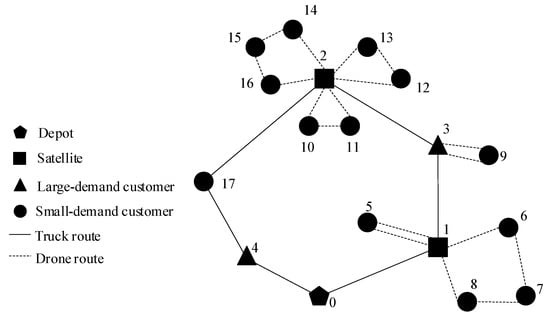
Figure 1. Illustration of the FMTDJRP.

Consider a network $G=(N,A)$, where N is the set of nodes and A is the set of arcs. The set $N=O\cup K\cup C$ includes the following:

• The depot O, with $o_s$ and $o_e$, respectively, denoting the start and end of the truck route;
• The satellites K, where a truck can stop to launch and retrieve drones;
• The customers C.

Due to the limited load capacity of drones, the customer set C is divided into two subsets:

• $C^D$: Small-demand customers whose demand is within drone capacity; they can be visited by either the truck or drones.
• $C^T$: Large-demand customers whose demand exceeds the drone capacity; they must be visited by truck only.

To improve efficiency by utilizing the waiting time while unloading heavy goods from the truck, drones are also allowed to take off and land at large-demand customers $i\in C^T$. Therefore, the set of all truck–drone rendezvous nodes is defined as $F=K\cup C^T$.

  The following operating conditions are assumed:

• A single truck carrying a fleet of drones travels through the network.
• Each drone can take off at most once at a rendezvous node $f\in F$ and must return to the same node after completing its deliveries.
• A drone can serve multiple customers in a single sortie, subject to load capacity and flight range constraints.
• All the customers are visited exactly once, and each satellite can be visited at most once by the truck.
• Drones are fully charged before each launch.
• The truck’s load capacity and maximum trip distance are assumed to be non-limiting, i.e., negligible compared to drone constraints.

To formulate the problem mathematically, we now introduce the sets, parameters, and decision variables, as shown in Table 3.

Table 3. Notations.

Notation	Description
Sets
N	Set of nodes
A	Set of arcs
O	Subset of depots, $O=\{o_s,o_e\}$
K	Subset of satellites
C	Subset of customers, where $C=C^T\cup C^D$ and $C^T\cap C^D=\varnothing$
$C^D$	Subset of small-demand customers
$C^T$	Subset of large-demand customers
F	Subset of rendezvous nodes, $F=K\cup C^T$
P	Subset of nodes apart from depots, $P=K\cup C$
D	Set of drones
Parameters
$r^d$	Flight range of a drone
$s_{ij}$	Distance of arc $(i,j)\in A$
$q_i$	Demand of customer $i\in C$
v	Load capacity of a drone
$cd$	Unit travel cost for a drone
$ct$	Unit travel cost for the truck
Variables
$x_{ij}$	Binary variable indicating if the truck traverses arc $(i,j)\in A$
$z_{fdij}$	Binary variable indicating if drone d launched from node f traverses arc $(i,j)\in A$
$u_i$	Integer variable indicating the visiting order of node i in the truck route
$w_{ijd}$	Continuous variable indicating accumulative delivery amount of drone d on arc $(i,j)\in A$
$l_{ijd}$	Continuous variable indicating accumulative traveled distance of drone d on arc $(i,j)\in A$

It is worth noting that the FMTDJRP can be employed in the case with limited available drones, such as a start-up logistics company owning insufficient drones. Consider the set D as the set of drone sorties at each rendezvous node so that $\left|D\right|$ is the maximal number of allowed sorties at each rendezvous node, and relax the constraint on the launch/retrieve operation number of a drone at each rendezvous node, by which a single drone is allowed to be launched several times and carry out more delivery missions.

The mathematical formulation is as below:

Objective function:

$$\begin{array}{cc}\hfill min& ct\sum _{i\in P\cup \left\{o_s\right\}}\sum _{j\in P\cup \left\{o_e\right\}}{x}_{ij}{s}_{ij}+cd\sum _{i\in F\cup C^D}\sum _{j\in F\cup C^D}\sum _{f\in F}\sum _{d\in D}{z}_{fdij}{s}_{ij}\hfill \end{array}$$

(1)

Subject to the following:

$$\begin{array}{c}\hfill \sum _{j\in P,j\ne i}{x}_{ij}=\sum _{j\in P,j\ne m}{x}_{jm},i=o_s,m=o_e\end{array}$$

(2)

$$\begin{array}{c}\hfill \sum _{i\in P\cup \left\{o_s\right\},i\ne j}{x}_{ij}=\sum _{m\in P\cup \left\{o_e\right\},m\ne j}{x}_{jm},\forall j\in P\end{array}$$

(3)

$$\begin{array}{c}\hfill \sum _{i\in F\cup C^D,i\ne j}{z}_{fdij}=\sum _{m\in F\cup C^D,j\ne m}{z}_{fdjm},\forall d\in D,j\in C^D,f\in F\end{array}$$

(4)

$$\begin{array}{c}\hfill \sum _{i\in \left\{o_s\right\}\cup P,i\ne j}{x}_{ij}\le 1,\forall j\in K\end{array}$$

(5)

$$\begin{array}{c}\hfill \sum _{i\in \left\{o_s\right\}\cup P,i\ne j}{x}_{ij}=1,\forall j\in C^T\end{array}$$

(6)

$$\begin{array}{c}\hfill \sum _{f\in F}\sum _{d\in D}\sum _{j\in F\cup C}{z}_{fdij}+\sum _{j\in \left\{o_e\right\}\cup P,i\ne j}{x}_{ij}=1,\forall i\in C^D\end{array}$$

(7)

$$\begin{array}{c}\hfill M(x_{ij}-1)+u_i+1\le u_j,\forall i\in P\cup \left\{o_s\right\},j\in P\cup \left\{o_e\right\}\end{array}$$

(8)

$$\begin{array}{c}\hfill 1\le u_i\le \left|P\right|+2,\forall i\in P\cup O\end{array}$$

(9)

$$\begin{array}{c}\hfill z_{fdij}\le \sum _{m\in C}{z}_{fdfm},\forall d\in D,i,j\in C^D\cup F,i\ne j,f\in F\end{array}$$

(10)

$$\begin{array}{c}\hfill z_{fd{f}^{\prime }j}=0,\forall d\in D,f\in F,j\in F\cup C^D,f^{\prime }\in \{F:f\ne f^{\prime }\}\end{array}$$

(11)

$$\begin{array}{c}\hfill z_{fdf{f}^{\prime }}=0,\forall d\in D,f,f^{\prime }\in F\end{array}$$

(12)

$$\begin{array}{c}\hfill z_{fdfj}\le \sum _{i\in P\cup \left\{o_s\right\}}{x}_{if},\forall f\in F,d\in D,j\in C^D\end{array}$$

(13)

$$\begin{array}{c}\hfill \sum _{j\in C^D}{z}_{fdfj}=\sum _{j\in C^D}{z}_{fdjf}\le 1,\forall f\in F,d\in D\end{array}$$

(14)

$$\begin{array}{c}\hfill l_{fjd}=d_{fj}{z}_{fdfj},\forall f\in F,j\in C^D,d\in D\end{array}$$

(15)

$$\begin{array}{c}\hfill l_{ijd}\le s_{ij}+l_{mid}+M(2-z_{fdij}-z_{fdmi}),\forall i\in C^D,m\in P:m\ne i,j\in P:j\ne i,f\in F,d\in D\end{array}$$

(16)

$$\begin{array}{c}\hfill l_{ijd}\ge s_{ij}+l_{mid}-M(2-z_{fdij}-z_{fdmi}),\forall i\in C^D,m\in P:m\ne i,j\in P:j\ne i,f\in F,d\in D\end{array}$$

(17)

$$\begin{array}{c}\hfill l_{ijd}\le M\sum _{f\in F}{z}_{fdij},\forall i,j\in C^D\cup F,d\in D\end{array}$$

(18)

$$\begin{array}{c}\hfill l_{ijd}\le r,\forall i,j\in C^D\cup F,f\in F,d\in D\end{array}$$

(19)

$$\begin{array}{c}\hfill w_{fjd}=0,\forall f\in F,j\in C^D,d\in D\end{array}$$

(20)

$$\begin{array}{c}\hfill w_{ijd}\le q_i+w_{mid}+M(2-z_{fdij}-z_{fdmi}),\forall i\in C^D,m\in P:m\ne i,j\in P:j\ne i,f\in F,d\in D\end{array}$$

(21)

$$\begin{array}{c}\hfill w_{ijd}\ge q_i+w_{mid}-M(2-z_{fdij}-z_{fdmi}),\forall i\in C^D,m\in P:m\ne i,j\in P:j\ne i,f\in F,d\in D\end{array}$$

(22)

$$\begin{array}{c}\hfill w_{ijd}\le M\sum _{f\in F}{z}_{fdij},\forall i,j\in C^D\cup F,d\in D\end{array}$$

(23)

$$\begin{array}{c}\hfill w_{ijd}\le v,\forall i,j\in C^D\cup F,f\in F,d\in D\end{array}$$

(24)

The objective function given in (1) aims to minimize the total travel cost for delivery. The first term represents the cost of the truck route and the second term the cost of drone routes. Both of them are proportional to the traveled distance.

Constraint (2) shows that the truck must visit other nodes except the depot once it starts its tour and must return to the depot in the end. Constraints (3) and (4) ensure flow conservation at each node. Constraint (5) indicates that a satellite can be visited by the truck at most once. In other words, a satellite can be removed from the truck route if that lowers the total cost.

Constraints (6) and (7) together guarantee high service quality of the network. Specifically, (6) forces each large-demand customer to be visited by the truck exactly once because their demands exceed the load capacity of drones. Constraint (7) ensures that each small-demand customer will be served once, either by the truck or by a drone.

Constraints (8) and (9) eliminate subtours for the truck.

Constraints (10)–(14) ensure the feasibility of all the drone routes. The variable $z_{fdij}$ is a complex decision variable indicating the matching relation among a rendezvous node, a drone, and an arc.

Constraint (10) means that the corresponding matching relation fails if drone d is not launched at rendezvous node f. Constraints (11) and (12) make sure that a drone does not pass by and land at a rendezvous node other than the one where it is launched.

For technical reasons, drones are not able to carry out independent long-distance heavy-load trips, in that they are mounted on the truck when there are no delivery tasks for drones. If a drone needs to take off for delivery, the truck will transport it to a rendezvous node and wait there, which is defined by constraint (13). The launch/retrieve operation for each drone is limited to no more than once at each rendezvous node, as stated in constraint (14).

Constraints (15)–(17) help to track the traveled distance for each drone. Constraint (18) forces $l_{ijd}$ to be zero if drone $d\in D$ does not go through arc $(i,j)\in A$. Constraint (19) ensures that drones do not exceed their flying range.

Constraints (20)–(22) keep track of the accumulative delivery amount for each drone. Similar to (18), constraint (23) forces $w_{ijd}$ to be zero if drone $d\in D$ does not go through arc $(i,j)\in A$. Finally, constraint (24) ensures that the load capacity of drones is not violated.

4. Solution Methodology

The FMTDJRP is NP-hard because it becomes a traveling salesman problem (TSP) if the number of available drones is reduced to 0. It is difficult for MILP solvers such as GUROBI to find the optimum within a reasonable time, so the ALNS is developed to find near-optimal solutions.

The metaheuristic is chosen for its simplicity, as its calibration process is limited, and its robustness, as its structure allows itself to avoid the local optimum trap. The readers are referred to [32] for more details about the ALNS. The outline of the algorithm is given in Algorithm 1.

Starting from an initial solution x, the metaheuristic explores the search space by destructing and reconstructing the current solution $\overline{x}$ iteratively. As a key mechanism in ALNS for avoiding local optima, the functions SelectDestroyOperator and SelectRepairOperator determine which operators are employed in each iteration.

These functions use a roulette wheel mechanism, as shown in Equations (25) and (26), where ${\mathrm{prob}}_{{\omega }^{-}}$ and ${\mathrm{prob}}_{{\omega }^{+}}$ denote the probability of selecting destroy operator ${\omega }^{-}\in {\Omega }^{-}$ and repair operator ${\omega }^{+}\in {\Omega }^{+}$, respectively. Their cumulative scores are represented by ${\delta }_{{\omega }^{-}}\in {\Delta }^{-}$ and ${\delta }_{{\omega }^{+}}\in {\Delta }^{+}$:

$$\begin{array}{cc}\hfill {\mathrm{prob}}_{{\omega }^{-}}& ={\displaystyle \frac{{\delta }_{{\omega }^{-}}}{{\sum }_{{\omega }^{-}\in {\Omega }^{-}}{\delta }_{{\omega }^{-}}}}\hfill \end{array}$$

(25)

$$\begin{array}{cc}\hfill {\mathrm{prob}}_{{\omega }^{+}}& ={\displaystyle \frac{{\delta }_{{\omega }^{+}}}{{\sum }_{{\omega }^{+}\in {\Omega }^{+}}{\delta }_{{\omega }^{+}}}}\hfill \end{array}$$

(26)

The acceptance of the newly produced solution $x^{\prime }$ is determined by the Metropolis criterion, which has been proven to enhance the performance of ALNS-based algorithms [33]. A new solution $x^{\prime }$ that improves the objective value is always accepted. Otherwise, it is accepted with a probability given by the following:

$$exp\left({\displaystyle \frac{f\left(\overline{x}\right)-f\left(x^{\prime }\right)}{T}}\right)$$

where T is a temperature parameter used to gradually reduce the acceptance of worse solutions and avoid being trapped in local optima. The initial temperature $T_0$ is set to 20% of the total cost of the initial solution, and it decreases as iterations proceed.

At the end of each iteration, the cumulative scores ${\delta }_{{\omega }^{-}}$ and ${\delta }_{{\omega }^{+}}$ are updated according to Equations (27) and (28). Here, ${\delta }_{{\omega }^{-}}^{\prime }$ and ${\delta }_{{\omega }^{+}}^{\prime }$ are the current scores, $\lambda$ is the decay parameter, and $\psi$ is the reward score assigned based on operator performance. We set $\lambda =0.9$, and the values of $\psi$ are given in Table 4.

$$\begin{array}{cc}\hfill {\delta }_{{\omega }^{-}}& =\lambda {\delta }_{{\omega }^{-}}^{\prime }+(1-\lambda )\psi \hfill \end{array}$$

(27)

$$\begin{array}{cc}\hfill {\delta }_{{\omega }^{+}}& =\lambda {\delta }_{{\omega }^{+}}^{\prime }+(1-\lambda )\psi \hfill \end{array}$$

(28)

Algorithm 1: Outline of the ALNS

Table 4. Values of the reward scores $\psi$.

Value	Description
50	If the new solution is accepted as the best-known solution
30	If the new solution is accepted due to its better cost than the current one
15	If the new solution is accepted despite its worse cost than the current one
5	If the new solution is rejected

4.1. Solution Representation

A solution is encoded using three groups of arrays:

• Group 1: This group consists of a single array with two tiers and $|C^D|$ positions. It represents the matching relation between small-demand customers and their assigned service vehicle. If a small-demand customer is served by the truck, the corresponding position is set to $-1$; otherwise, it contains the index of the rendezvous node from which the drone is launched to serve the customer.
• Group 2: This group is a one-tier array representing the truck route. All large-demand customers must appear in this array. Satellites and small-demand customers may appear in the truck route, but their presence is not mandatory. The array starts and ends with the depot index.
• Group 3: This group contains several one-tier arrays, each corresponding to a drone route. The arrays are sorted based on the rendezvous nodes from which each drone route begins and ends.

Figure 2 demonstrates a solution encoded according to the network illustrated in Figure 1.

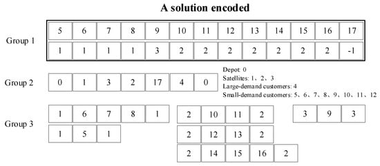
Figure 2. Example of a solution encoded.

The objective function is defined as follows:

$$f\left(x\right)=c\left(x\right)+\mu ·p\left(x\right)$$

(29)

where $c\left(x\right)$ denotes the total travel cost and $p\left(x\right)$ is the penalty cost associated with violating the number of drones employed. $\mu$ is the corresponding penalty weight. Other constraints, such as drone flight range and load capacity, are handled during the repair process.

4.2. A Knowledge-Based Acceleration Strategy (KAS)

As illustrated in Figure 3, certain drone arcs are inherently infeasible regardless of the rendezvous node from which the drone is launched, typically due to the remote location of the small-demand customer. Consequently, constructing such arcs throughout the entire optimization process is unnecessary. By excluding these infeasible arcs, the solution space is significantly reduced, thereby accelerating the metaheuristic search.

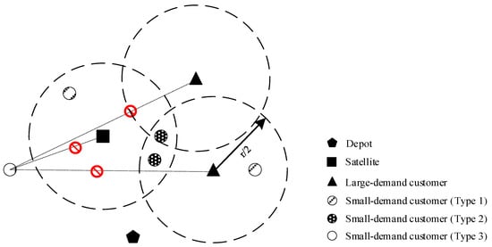
Figure 3. Illustration of the knowledge-based acceleration strategy.

To implement this idea, small-demand customers are pre-classified into three types before the search begins. The coverage radius of each rendezvous node is set to $0.5r$. If there exists a rendezvous node from which a drone can reach a small-demand customer without violating the flying range constraint, the node is called a potential rendezvous node for that customer.

• Type 1 customers ($C^1$): Have exactly one potential rendezvous node.
• Type 2 customers ($C^2$): Have more than one potential rendezvous node.
• Type 3 customers ($C^3$): Have no potential rendezvous node.

For customers of Type 1 and 2, the algorithm attempts to build drone arcs between them and their potential rendezvous nodes or inserts them into the existing drone routes linked to those nodes. For customers of Type 3, the algorithm only considers inserting them into the truck route.

This knowledge-based acceleration strategy is applied during the construction of the initial solution and throughout the repair process.

4.3. Initial Solution

To construct an initial solution, an order-first split-second heuristic is applied in the GenerateInitSol function. The steps are as follows:

• Assign every small-demand customer of Type 1 and Type 2 to their closest rendezvous node.
• Construct a giant TSP tour involving the rendezvous nodes with attached small-demand customers.
• Partition the tour into feasible drone routes, considering both flight range and load capacity constraints. The constraint on the number of available drones is relaxed in this step.
• Build the truck route by linking all the rendezvous nodes involved in drone routes and the small-demand customers of Type 3.

4.4. Destroy Operators

Given that the truck’s travel cost is usually higher than that of drones, opportunities for improving drone route sequences may be overlooked, especially when the cost difference between truck and drones is substantial. To address this, two variants are introduced for several destroy operators. Their illustration is shown in Figure 4.

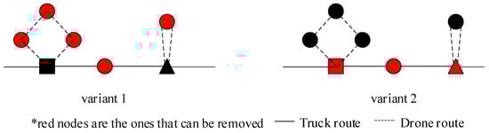
Figure 4. Illustration of the two variants of destroy operator.

Variant 1 targets small-demand customers, regardless of their current location in the solution. Variant 2 targets all the nodes situated in the truck route.

It is worth noting that small-demand customers in the truck route can be destroyed by both variants. Since the total cost is sensitive to whether they are assigned to truck or drone, increasing the frequency of destruction improves the chance of finding better placements.

For all node-based destroy operators, the destruction degree $\theta$ (i.e., the number of nodes to be removed) is a critical parameter. It is randomly drawn from the following interval:

$$\theta \in \left[0.1·\left|\mathrm{target}\mathrm{nodes}\right|,0.2·\left|\mathrm{target}\mathrm{nodes}\right|\right]$$

4.4.1. Random Destroy

Originally proposed by [34], the operator selects $\theta$ nodes at random and places them into the node pool. This is adapted for both Variant 1 and Variant 2.

4.4.2. Worst Destroy

Also adopted from [34], this operator removes the $\theta$ nodes that yield the highest removal gain. Let node j be the target node, and i, k its predecessor and successor, respectively. The removal gain is computed as follows:

$${\mathrm{Gain}}_j=\left\{\begin{array}{cc}{c}_d·(s_{ij}+s_{jk}-s_{ik}),\hfill & \mathrm{if}j\mathrm{is}\mathrm{in}\mathrm{a}\mathrm{drone}\mathrm{route}\hfill \\ c_t·(s_{ij}+s_{jk}-s_{ik}),\hfill & \mathrm{if}j\mathrm{is}\mathrm{in}\mathrm{the}\mathrm{truck}\mathrm{route}\hfill \end{array}\right.$$

4.4.3. Related Destroy

Based on [35], this operator also supports both variants. It randomly selects a seed node and then eliminates the $\theta -1$ nodes closest to it.

4.4.4. Similar Destroy

Adapted from [36], this operator is designed to destroy similar nodes. The similarity between nodes i and j is calculated as follows:

$$\Pi (i,j)=\alpha ·{\overline{s}}_{ij}+\beta ·\left|{\overline{q}}_i-{\overline{q}}_j\right|$$

where ${\overline{s}}_{ij}$ is the normalized distance; ${\overline{q}}_i$ is the normalized demand; and $\alpha$, $\beta$ are the corresponding weights. Since it incorporates demand information, this operator is only applied to small-demand customers.

4.4.5. Route Destroy

Inspired by [37], this operator removes a complete drone route and sends all its small-demand customers to the node pool. The connected rendezvous node remains temporarily in the truck route. If it is a satellite and remains unused after the repair process, it is deleted from the truck route. This operator is disabled when no drone route exists.

4.4.6. Satellite Opening

Based on [35], this operator addresses the risk that some neighborhoods may never be explored if satellites are permanently removed. It randomly selects a satellite currently not in the truck route, and then removes the $\theta$ closest small-demand customers to that satellite and adds them to the node pool.

4.5. Repair Operators

As described in Section 4.4, the destroy process removes not only customers but also satellites. Unlike previous studies, our repair process is responsible for reinserting all these components together, allowing the optimization of the network in an integrated manner.

After the insertion, some satellites may end up with no connected drone routes, which implies that their presence in the truck route is redundant. In such cases, the repair operators will further eliminate these empty satellites.

4.5.1. Greedy Insertion

Nodes are inserted one by one in a random sequence into the position with the lowest insertion cost.

For satellites, large-demand customers, and small-demand customers of Type 3, they must be assigned to the truck route. Thus, we attempt to insert them using the SearchTruckRoute function.

For other nodes—namely small-demand customers of Type 1 and Type 2—we attempt the following:

• Insertion into the truck route via SearchTruckRoute;
• Insertion into drone routes via SearchDroneRoute, which includes either of the following:

  –

  Adding to an existing drone route associated with a potential rendezvous node;

  –

  Creating a new drone route from that rendezvous node.

SearchDroneRoute checks feasibility in terms of flight range and drone load capacity. The framework of this repair operator is illustrated in Algorithm 2.

Algorithm 2: Framework of greedy insertion

4.5.2. Perturbed Greedy Insertion

This operator adopts the same structure as the greedy insertion operator but introduces randomness by applying a noise factor $\epsilon$ to the insertion cost.

The perturbed cost helps avoid always choosing the same position, thus improving diversity in the search space. The noise factor $\epsilon$ is randomly selected from the interval $[0.8,1.2]$, as suggested by [35].

4.5.3. Regret Insertion

The regret insertion operator computes the regret value of all the nodes in the pool and inserts the one with the highest regret value. After that, the operator repeats the process for the nodes left in the pool until the pool is empty. The regret value $R{V}_i$ of node i is calculated as follows:

$$R{V}_i=I_i^2-I_i^1$$

(30)

where $I_i^k$ denotes the k-th cheapest insertion cost for node i.

This mechanism compensates for the myopia of the greedy insertion by avoiding situations where the last few nodes in the node pool can only be inserted into poor positions.

Similar to the greedy insertion, if node i is one of the satellites, large-demand customers, or small-demand customers of Type 3, all of its insertion costs $I_i^k$ are only related to the truck route, and are computed by ComputeRV_A. As for the remaining nodes (i.e., small-demand customers of Type 1 and Type 2), their insertion costs are related to both the truck and drone routes, and are computed by ComputeRV_B.

The framework of this operator is given in Algorithm 3.

Algorithm 3: Framework of regret insertion

4.6. Local Search

The local search is executed every $\mathit{freq}$ iterations, where $\mathit{freq}$ is set to 5000 in our algorithm. During local search, the truck route and the drone routes are treated as a simple traveling salesman problem (TSP) tour. The change in service vehicle for a node is not considered, as this would significantly increase the complexity of the neighborhood structure.

The purpose of local search is to make subtle adjustments to the existing solution, which may be masked during the destroy-and-repair phases. To this end, a series of classical heuristics are employed, including 2-opt, relocate, and exchange, as illustrated in Figure 5.

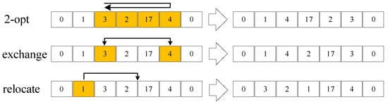
Figure 5. Illustrations of local search heuristics.

5. Experimental Results and Analysis

The mathematical model presented in Section 2 was solved by Gurobi 9.1, while the ALNS algorithm introduced in Section 3 was implemented in Python 3.8. All the computational experiments were conducted on an ASUS laptop equipped with an AMD Ryzen 7 4800H processor (2.90 GHz) and 16 GB of RAM.

5.1. Test Instances

Due to the lack of publicly available real-life truck–drone delivery data, all the benchmark instances were generated based on the Solomon benchmark dataset and the Gehring & Homberger dataset. These datasets are widely used in the literature for the Vehicle Routing Problem with Time Windows (VRPTW), and contain up to 100 and 200 customer nodes, respectively.

Given that the FMTDJRP network involves the presence of satellites, the Solomon dataset does not suffice for generating large-scale instances. Therefore, we used the Solomon dataset for small-scale test instances and the Gehring & Homberger dataset for large-scale instances.

The instance generation process proceeded as follows: First, n customer nodes were selected from a source instance. Then, m out of these n nodes were randomly designated as large-demand customers, and the remaining nodes as small-demand customers. Additionally, p nodes were selected as satellites from the same instance. The satellites were chosen to be spatially distant from one another and located near the centroid of customer-dense regions.

It is worth noting that approximately 86% of the goods delivered by Amazon weigh less than 5 lbs [38], which is below the load capacity of drones. Accordingly, for large-scale instances, we set the ratio $m/n=0.1$.

Both the Solomon and Gehring & Homberger datasets contain three categories of instances based on node distribution: random (R), clustering (C), and random+clustering (RC). Therefore, our generated instances reflect these three distribution scenarios. The naming convention follows the pattern Type_Scale_No, where Type $\in$ {C, R, RC}, Scale $\in$ {S (small), L (large)}. Table 5 and Table 6 give the information about the generated instances.

Table 5. Information about small-scale instances.

Instance	Source Instance	n	m	p
C_S_1	Solomon C101	8	1	2
C_S_2	Solomon C101	15	2	3
C_S_3	Solomon C101	20	3	4
C_S_4	Solomon C201	8	1	2
C_S_5	Solomon C201	15	2	3
C_S_6	Solomon C201	20	3	4
R_S_1	Solomon R101	8	2	1
R_S_2	Solomon R101	15	2	4
R_S_3	Solomon R101	20	3	4
RC_S_1	Solomon RC101	8	2	1
RC_S_2	Solomon RC101	15	3	3
RC_S_3	Solomon RC101	20	3	4

Table 6. Information about large-scale instances.

Instance	Source Instance	n	m	p
C_L_1	Gehring & Homberger C1_2_1	30	3	3
C_L_2	Gehring & Homberger C1_2_1	40	4	4
C_L_3	Gehring & Homberger C1_2_1	50	5	5
C_L_4	Gehring & Homberger C1_2_1	60	6	6
C_L_5	Gehring & Homberger C1_2_1	70	7	7
C_L_6	Gehring & Homberger C1_2_1	80	8	8
C_L_7	Gehring & Homberger C1_2_1	90	9	9
C_L_8	Gehring & Homberger C1_2_1	100	10	10
R_L_1	Gehring & Homberger R1_2_1	30	3	4
R_L_2	Gehring & Homberger R1_2_1	40	4	4
R_L_3	Gehring & Homberger R1_2_1	50	5	5
R_L_4	Gehring & Homberger R1_2_1	60	6	6
R_L_5	Gehring & Homberger R1_2_1	70	7	7
R_L_6	Gehring & Homberger R1_2_1	80	8	8
R_L_7	Gehring & Homberger R1_2_1	90	9	9
R_L_8	Gehring & Homberger R1_2_1	100	10	10
RC_L_1	Gehring & Homberger RC1_2_1	30	3	3
RC_L_2	Gehring & Homberger RC1_2_1	40	4	4
RC_L_3	Gehring & Homberger RC1_2_1	50	5	5
RC_L_4	Gehring & Homberger RC1_2_1	60	6	6
RC_L_5	Gehring & Homberger RC1_2_1	70	7	7
RC_L_6	Gehring & Homberger RC1_2_1	80	8	8
RC_L_7	Gehring & Homberger RC1_2_1	90	9	9
RC_L_8	Gehring & Homberger RC1_2_1	100	10	8

Given the technical limitations, drones are currently incapable of performing independent long-distance deliveries with heavy loads. Based on preliminary tests, the drone flight range r was set to 25 units, and the load capacity v was set to 60 units. Under these constraints, customers served by drones are expected to be located in close proximity to the rendezvous nodes.

The number of available drones was assumed to be three. The unit travel cost for drones $c_d$ and for the truck $c_t$ was set to 1 and 8, respectively. This cost ratio between drones and trucks ($c_d:c_t=1:8$) was adopted from the study by Salama and Srinivas [31].

5.2. Comparison of the ALNS with GUROBI

Since the FMTDJRP belongs to NP-hard problems, commercial solvers such as GUROBI cannot find the optimal solution within a reasonable time. We used only small-scale instances to compare the performance of GUROBI and the ALNS. The maximal execution time for GUROBI was set to 7200 s and the maximal iterations for the ALNS was set to 5000. The results are reported in Table 7.

Table 7. Comparison of the ALNS with GUROBI.

Instance	GUROBI ${\mathit{c}}_{\mathbf{total}}$	GUROBI T (s)	ALNS ${\mathit{c}}_{\mathbf{total}}$	ALNS T (s)	Gap (%)
C_S_1	400.45	145.00	400.45	2.15	0.00
C_S_2	700.03	7200.00 *	700.03	2.53	0.00
C_S_3	1028.71	7200.00 *	1028.71	2.68	0.00
C_S_4	388.15	3.01	388.15	2.21	0.00
C_S_5	749.16	7200.00 *	749.16	2.48	0.00
C_S_6	1228.42	7200.00 *	1228.42	2.70	0.00
R_S_1	1598.09	0.21	1598.09	2.15	0.00
R_S_2	1658.69	517.00	1658.69	2.41	0.00
R_S_3	1856.97	7200.00 *	1856.97	2.61	0.00
RC_S_1	1092.46	4.11	1092.46	2.11	0.00
RC_S_2	1327.35	7200.00 *	1327.35	2.42	0.00
RC_S_3	1602.30	7200.00 *	1602.30	2.76	0.00

* Optimality not proven when the execution time limit was reached.

The good performance of the ALNS is shown in the results. For the instances whose optimality is obtained by GUROBI, the ALNS can also find their optimality. For those whose optimality is not obtained by GUROBI within a reasonable time, the ALNS can find the solution not worse than those of GUROBI.

The ALNS outperforms GUROBI in terms of execution time. It can be observed that the instances with clustering distribution characteristics are more difficult for GUROBI to solve. For example, C_S_2, C_S_5, and RC_S_2 all have only seven more customers and one more satellite than C_S_1, C_S_4, and RC_S_1, but the execution time increases sharply. For the instances of type R, this dramatic increase in execution time does not appear until the number of customers becomes 20.

Such surge in execution time with the increase in customers is not observed in the ALNS results, and all small instances can be solved in less than 3 s.

5.3. Performance of the ALNS for Large-Scale Instances

Before the tests for large-scale instances, a pre-test to parameterize the number of iterations for the ALNS was first performed. As known to all, for metaheuristics, the number of iterations has a great impact on the quality of solutions to some degree. More iterations mean more execution time, but are also more likely to obtain a better solution.

In order to achieve a relatively satisfying trade-off between the quality of solutions and the execution time, three different stop criteria as shown in Table 8 were tested. Each criterion has three characteristics: Iter_Max represents the maximal number of iterations; Check_Length means that if the current best solution has not been updated for this number of iterations, the search stops; and Check_Start ensures that the search must not stop until this number of iterations is reached, which gives more chances to the metaheuristic to escape from the local optimum.

Table 8. Three stop criteria.

Criterion	Iter_Max	Check_Length	Check_Start
A	50,000	10,000	10,000
B	80,000	20,000	36,000
C	100,000	25,000	62,500

Criterion A performs well on all the instances with up to 60 customers. Therefore, three criteria were tested on all the instances with 100 customers. For each instance, the metaheuristic was run for 20 times with every stop criterion. The test results of the largest instances, which are C_L_8, R_L_8, and RC_L_8, are shown in Figure 6.

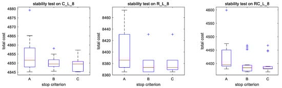
Figure 6. Test results for three iteration stop criteria.

When comparing the results of Criterion A and Criterion B in these three instances, one can find that the algorithm can find better solutions and be more stable with the increase in iterations. The ranges of the results obtained by Criterion B compared to those obtained by Criterion A decrease by 63.14%, 39.19%, and 54.90% for C_L_8, R_L_8, and RC_L_8, respectively. However, the ranges of the results obtained by Criterion C compared to those obtained by Criterion B decrease only by 4.46%, 0.00%, and 0.21%, respectively, and the best results obtained by Criterion B and Criterion C are very close.

Therefore, we chose Criterion A for all the instances with up to 60 customers and Criterion B for all the instances from 70 to 100 customers.

The results of the tests for large-scale instances are shown in Table 9. For each instance, the travel cost for the whole network ($c_{\mathrm{total}}$), the truck ($c_{\mathrm{truck}}$), and the drones ($c_{\mathrm{drone}}$) are reported. Two indicators concerning the delivery characteristic, namely the number of truck stops (#stop) and the ratio of drone service ($\phi$), are also given. The ratio of drone service is calculated as follows:

$$\phi ={\displaystyle \frac{\mathrm{NCSD}}{\left|C^D\right|}}$$

where NCSD represents the number of customers served by drones. The execution time of the metaheuristic for each instance is recorded in the column named T. The last column shows the cost savings $\mathit{sav}$ that the FMTDJRP makes compared to the corresponding truck-only situation. The cost saving is calculated as follows:

$$\mathit{sav}=1-{\displaystyle \frac{{\cos \mathrm{t}}_{\mathrm{FTDSRP}}}{{\cos \mathrm{t}}_{\mathrm{TO}}}}$$

where ${\cos \mathrm{t}}_{\mathrm{FTDSRP}}$ represents the total travel cost of the FMTDJRP, and ${\cos \mathrm{t}}_{\mathrm{TO}}$ represents the total travel cost of the corresponding truck-only situation.

Table 9. Results of ALNS for large-scale instances.

Instance	${\mathit{c}}_{\mathbf{total}}$	${\mathit{c}}_{\mathbf{truck}}$	${\mathit{c}}_{\mathbf{drone}}$	#Stop	$\mathit{\phi }$	T (s)	sav
C_L_1	1331.26	1232.78	98.48	13	0.67	7.19	0.23
C_L_2	1617.27	1435.24	182.03	17	0.69	9.71	0.26
C_L_3	2064.55	1825.64	238.91	22	0.69	13.72	0.23
C_L_4	2522.52	2220.43	302.09	24	0.72	22.71	0.23
C_L_5	3066.14	2735.92	330.22	28	0.73	76.10	0.19
C_L_6	3578.70	3205.61	373.09	29	0.76	156.42	0.19
C_L_7	4164.67	3761.89	402.78	34	0.77	327.02	0.17
C_L_8	4845.17	4382.68	462.49	37	0.79	379.70	0.18
Average ratio of drone service: 0.73; Average cost saving: 0.21
R_L_1	5721.36	5677.22	44.14	29	0.11	3.87	0.01
R_L_2	5940.18	5867.96	72.22	37	0.11	7.41	0.03
R_L_3	6621.27	6538.66	82.61	47	0.13	6.40	0.03
R_L_4	6728.82	6491.60	237.22	50	0.28	14.01	0.05
R_L_5	6845.49	6659.14	186.35	62	0.19	53.18	0.07
R_L_6	7736.87	7553.72	183.15	71	0.17	52.03	0.05
R_L_7	7725.95	7406.52	319.43	72	0.28	66.71	0.06
R_L_8	8373.19	8061.82	311.37	81	0.27	91.05	0.07
Average ratio of drone service: 0.19; Average cost saving: 0.04
RC_L_1	4269.37	4229.39	39.98	25	0.22	3.81	0.03
RC_L_2	4609.38	4488.06	121.32	25	0.47	9.31	0.06
RC_L_3	3719.19	3511.61	207.58	21	0.66	26.23	0.15
RC_L_4	4610.74	4414.47	196.27	32	0.57	50.33	0.09
RC_L_5	4557.80	4299.83	257.97	34	0.62	81.24	0.13
RC_L_6	4982.34	4796.28	186.06	39	0.61	186.07	0.16
RC_L_7	4679.31	4370.13	309.18	47	0.58	114.75	0.15
RC_L_8	4369.10	3943.36	425.74	37	0.76	330.51	0.19
Average ratio of drone service: 0.56; Average cost saving: 0.12

Four observations can be concluded from the results: First, the execution time increases as the instance size increases. Take instances of type C for example. When we take a closer look at the first four instances and the last four instances, respectively, we can still find this execution time increase despite the effect brought by different stop criteria. It can be also found that the execution time increase in the last four is sharper than the first four. Second, among the instances with the same number of customers but of different types, the instance of type R always needs the least execution time. The execution time needed for type C and type RC is close. Third, the instances of type C have the highest ratio of drone service. The instances of type RC have the second high ratio of drone service and those of type R have the lowest. Moreover, the ratio of drone service of type RC varies in a much larger range than others. From the smallest instance to the largest one, the difference between the maximal ratio and the minimal ratio reaches 0.55, while this difference is only 0.12 and 0.16, respectively, for type C and type R. Finally, the instances of type C have the highest average cost saving. The instances of type RC have the second high cost saving and those of type R have the lowest. Similar to the ratio of drone service, the cost saving of type RC varies in the largest range compared to others. From the smallest instance to the largest one, the difference between the maximal saving and the minimal saving reaches 0.16, while this difference is only 0.06 for both type C and type R.

5.4. Effect of the Knowledge-Based Acceleration Strategy

Embedded in the initialization process and the repair operators, the design of the KAS is based on the two-level structure of the FMTDJRP. Also, as a vital parameter, the coverage radius of each rendezvous node is set in accordance with our prior knowledge. Hence, in this section, we investigate the effect of this acceleration strategy and justify its parameter setting.

The experiments were conducted with the same instances and drone-truck related parameters used in the previous section except the configuration of the algorithm. Three modified configurations were considered: without the KAS (w/o KAS), with the KAS in which the coverage radius is set to 0.3r (w/KAS (0.3r)), and with the KAS in which the coverage radius is set to 0.4r (w/KAS (0.4r)). There was no need to investigate the coverage radius larger than 0.5r because of possible infeasible insertions of some small-demand customers. The results obtained by these three configurations were compared to those of the configuration used for the entire paper (i.e., with the KAS in which the coverage radius is set to 0.5r). Two aspects were examined, which are the cost gap ($c^{gap}$) calculated as

$$c^{gap}=\left({\displaystyle \frac{c_{total}^{\prime }}{c_{total}}}-1\right)\times 100\%$$

and the execution time gap ($t^{gap}$) calculated as

$$t^{gap}=\left({\displaystyle \frac{T^{\prime }}{T}}-1\right)\times 100\%$$

where $c_{total}^{\prime }$ and $T^{\prime }$ represent, respectively, the total cost obtained and the execution time needed with the modified configuration. The results are reported in Table 10.

Table 10. Results of the experiments on the KAS.

Instance	w/o KAS		w/KAS (0.3r)		w/KAS (0.4r)
	${\mathit{c}}^{\mathit{gap}}$ (%)	${\mathit{t}}^{\mathit{gap}}$ (%)	${\mathit{c}}^{\mathit{gap}}$ (%)	${\mathit{t}}^{\mathit{gap}}$ (%)	${\mathit{c}}^{\mathit{gap}}$ (%)	${\mathit{t}}^{\mathit{gap}}$ (%)
C_L_1	0.00	45.34	0.56	−18.50	0.00	−2.50
C_L_2	0.00	13.18	17.72	−16.27	2.62	0.10
C_L_3	0.00	24.13	11.14	−19.10	2.60	−11.73
C_L_4	−0.07	67.28	8.55	−38.09	1.74	−0.04
C_L_5	1.67	32.75	1.32	9.80	1.04	8.00
C_L_6	0.00	8.75	8.54	−35.89	0.45	−17.34
C_L_7	0.04	−11.75	3.59	−52.46	1.62	−53.07
C_L_8	0.05	32.20	3.50	−66.98	1.26	−31.26
R_L_1	0.34	37.47	0.25	−4.39	0.00	−2.84
R_L_2	0.65	−15.92	2.17	−13.50	0.55	−26.18
R_L_3	0.00	55.63	2.76	7.34	0.24	−0.78
R_L_4	−0.01	9.28	2.42	−22.06	2.12	−7.14
R_L_5	0.59	12.15	6.41	−26.25	1.09	−19.74
R_L_6	0.95	102.52	3.70	8.48	3.04	−6.96
R_L_7	0.36	56.62	3.08	−1.05	0.89	−3.57
R_L_8	0.00	105.26	5.17	−8.57	2.01	−0.48
RC_L_1	0.00	8.66	1.98	0.00	0.00	−3.41
RC_L_2	0.09	20.19	0.27	−45.01	0.00	−28.68
RC_L_3	0.00	−16.36	2.07	−51.12	1.83	−16.32
RC_L_4	0.00	18.94	1.10	−58.37	1.04	−12.20
RC_L_5	−0.02	67.17	1.76	−43.70	3.30	−5.88
RC_L_6	2.38	−1.59	6.13	−31.73	6.27	−11.40
RC_L_7	0.77	65.19	1.91	2.23	2.80	−16.24
RC_L_8	0.06	23.83	3.19	−54.90	0.59	−40.59

$c^{gap}<0$: the modified configuration yields a solution with a lower total cost; $t^{gap}<0$: the modified configuration yields a solution within a shorter time.

Two conclusions are given in the Table 10. First, the KAS is able to accelerate the metaheuristic and guarantee the solution quality in the meantime. Observing the column w/o KAS, we can find that $t^{gap}$ is larger than 10% for most of the instances and even surpasses 100% for some of them, which means the KAS reduces the execution time significantly. Meanwhile, $c^{gap}$ is very close to 0 for the majority of the instances, meaning that the total cost obtained by the metaheuristic with and without the KAS is almost the same. Second, the current setting of the coverage radius (equal to 0.5r) is reasonable. For the configurations w/KAS (0.3r) and w/KAS (0.4r), although the execution time is reduced significantly, the solution quality is degraded as well. However, this solution quality degradation is mitigated when the coverage radius becomes larger. As the results show, there is still room for improvement when the coverage radius is set to 0.4r. Since it is impossible for the distance between a small-demand customer and a rendezvous node to be over 0.5r, the current setting can be well-functioning.

5.5. Sensibility Analysis

5.5.1. Drone Features

The experiment in this section was conducted to explore how the flight range and the load capacity of drones influence the total cost in diverse customer distribution scenarios. We chose C_L_4, R_L_4 and RC_L_4 for the experiment. We varied the load capacity from 40 to 80 and the flight range from 25 to 65. The number of drones was still assumed to be three. The results shown in Figure 7 demonstrate the evolution of the cost saving (vertical axis) with various combinations of flight range (horizontal axis) and load capacity (horizontal axis). The cost saving is defined the same as in Section 5.3.

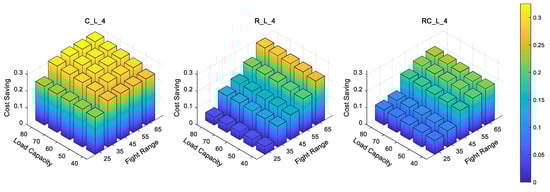
Figure 7. Test results for various combinations of drone features.

Figure 7 shows the flexibility of the FMTDJRP because it can adapt to all customer distribution scenarios and yield solutions with a cost saving larger than 0, which means these solutions are cheaper than those of truck-only situations. Clearly, the cost savings are much more significant when customers are distributed in clusters because the cost savings are higher than the two other customer distribution scenarios. However, for C_L_4, with the increase in the flight range and the load capacity of drones, the cost saving rises more gently. This is because each cluster of customers has a fixed radius and clusters are relatively far away from each other. Even though the flight range and the load capacity of drones increase, the areas that drones are able to cover stay relatively unchanged. In consequence, drones are not able to serve more customers after taking off from a rendezvous node.

On the contrary, the results are quite different in the random customer distribution scenario. When the load capacity and the flight range of drones are limited, the cost savings are less than 0.10, whereas with the increase in the flight range and the load capacity of drones, the cost saving rises steeply. Because in the random distribution scenario, customers are not grouped in clusters with a radius, the longer flight range and the larger load capacity enable drones to serve such more customers that the truck travels a much shorter distance. Since the unit travel cost of a truck is much higher than that of a drone, the shorter distance the truck travels, the lower the total travel cost is. One can also observe that the flight range is the leading factor in the cost saving rise.

The results of RC_L_4 have the duality of two customer distribution scenarios mentioned above. When the flight range is less than 35, there is no significant difference between the total travel cost of the FMTDJRP and that of the truck-only situations. Once the flight range is over 35, the cost saving becomes much more obvious. The reason for that is drones are only able to serve clustering customers when the flight range is limited, and the increase in the flight range enables drones to serve some randomly distributed customers so that the distance traveled by truck is reduced, which leads to the reduction in the total travel cost.

5.5.2. Unit Travel Cost of Truck and Drone

Still based on C_L_4, R_L_4 and RC_L_4, which represent three customer distribution scenarios, the experiments in this section were conducted to explore how the unit travel cost of truck and drone influences the cost saving and the ratio of drone service. The drone–truck unit cost ratios ranging from 1:2 to 1:32 were considered. The cost saving is defined the same as in Section 5.3.

As Figure 8 shows, the saving of the clustering distribution scenario is always the highest whatever the cost ratio is. With the decrease in the cost ratio, the saving for all distribution scenarios rises gradually. As for the ratio of drone service, the clustering distribution scenario is superior to others as well. Nevertheless, when the drone–truck unit cost ratio changes from 1:2 to 1:32, the ratio of drone service of the random distribution scenario (type R) rises by 153.8%, the fastest among three scenarios, followed by the random plus clustering distribution scenario (type RC) whose ratio of drone service rises by 80.5% and the clustering distribution scenario (type C) whose ratio of drone service rises by 77.3%.

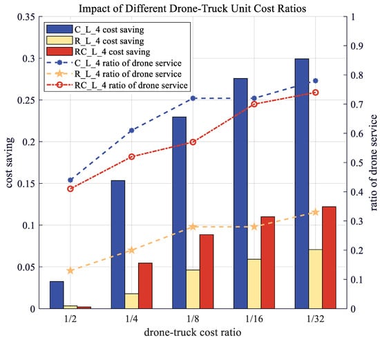
Figure 8. Impact of different drone–truck cost ratios.

This can be explained as follows: The low density of customers comes with their random distribution, which requires drones to fly a longer distance to serve a customer. With a relatively high drone–truck unit cost ratio, the cost of using a drone or the truck for a delivery is close. But when the drone–truck unit cost lowers, the cost of drone service becomes significantly cheaper than truck service; thus, launching a drone to serve customers instead of a truck is much more preferred.

5.5.3. Truck Access to Small-Demand Customers

In order to demonstrate the flexibility of the FMTDJRP and the necessity of allowing the truck to visit small-demand customers, the experiments in this section were carried out as follows:

First, a normal multi-visit truck and drone joint routing problem (NMTDJRP) was defined. In the NMTDJRP, all small-demand customers must be served by drones and the truck has no access to small-demand customers. Other constraints were exactly the same as the FMTDJRP. Then, we used the same instances to solve the FMTDJRP and the NMTDJRP with three different combinations of drone features. After that, the failure ratio (FR) was computed for each instance solved in the context of the NMTDJRP. As an adaptability indicator, FR is defined as

$$FR={\displaystyle \frac{USC}{\left|C^D\right|}}$$

where $USC$ means the number of unserved customers. The lower $FR$ is, the more adaptable to the corresponding instance the NMTDJRP is. In the case of $FR=0$, the NMTDJRP yields a full solution in which all customers are served. Finally, for all instances where the NMTDJRP can yield a full solution, the total travel cost of the FMTDJRP and that of the NMTDJRP were compared.

When focusing on the result of each combination in Figure 9, one can observe that $FR$ shows a downward trend with the increase in the number of customers. In addition, $FR$ of the clustering distribution scenario is always the lowest, which means the NMTDJRP suits this scenario the best. In contrast, the NMTDJRP suits the random distribution scenario the worst as its $FR$ is the highest for each combination. The trend of $FR$ for the clustering distribution scenario is reversed at some point because of the appearance of several relatively faraway customers. When observing three combinations together, it can be found that $FR$ of every distribution scenario decreases overall with the increase in the flight range and the load capacity. As it can be seen, $FR$ for the random distribution scenario decreases the most significantly. Even though the NMTDJRP adapts to more instances with the higher load capacity and the longer flight range, it is still not competitive with the FMTDJRP that can always adapt to any customer distribution scenario no matter the drone features.

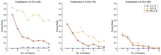
Figure 9. NMTDJRP failure ratio in each combination of drone features.

In terms of cost saving, the FMTDJRP outperforms the NMTDJRP as well. For those instances where both FMTDJRP and NMTDJRP can yield full solutions, reported in Table 11 are the total travel cost of each and the cost gaps calculated as

$$Gap=\left(1-{\displaystyle \frac{c_F}{c_N}}\right)\times 100\%$$

where $c_F$ and $c_N$ represent, respectively, the total cost for the FMTDJRP and the NMTDJRP.

Table 11. Comparison of the total travel cost of the FMTDJRP and NMTDJRP.

Instance	${\mathit{c}}_{\mathit{F}}$	${\mathit{c}}_{\mathit{N}}$	Gap (%)
Combination 1
C_L_1	1331.26	1394.01	4.50
C_L_2	1617.27	1742.17	7.17
Combination 2
C_L_1	1322.87	1353.47	2.26
C_L_2	1583.22	1635.27	3.18
C_L_3	1816.22	1868.74	2.81
C_L_4	2247.78	2292.83	1.96
C_L_5	2808.29	2910.00	3.50
C_L_6	3288.53	3317.36	0.87
C_L_7	3872.31	3904.57	0.83
Combination 3
C_L_1	1325.16	1346.14	1.56
C_L_2	1576.80	1699.01	7.19
C_L_3	1792.66	1855.04	3.36
C_L_4	2216.03	2273.61	2.53
C_L_5	2773.28	2814.37	1.46
C_L_6	3259.39	3292.85	1.02
C_L_7	3840.71	3880.06	1.01
RC_L_7	3515.99	3590.46	2.07
RC_L_8	3663.32	3747.68	2.25

One can find that the gaps are all positive, which means whenever a full solution is obtained, the FMTDJRP solution is always cheaper than the NMTDJRP solution. This can be explained by Figure 10 the solutions of the FMTDJRP and the NMTDJRP to C_L_2 with drone feature combination 3. In the NMTDJRP solution, all small-demand customers are visited by drones. This task allocation strategy can indeed reduce the distance traveled by the truck so as to reduce the total cost but not always. For example, the cost of adding customer a into the truck tour is +3.10. In the meanwhile, the cost of removing customer a from the drone tour connected to large-demand customer b (functioning as a rendezvous node here) is −10.56. Consequently, a cost saving of 7.46 is created. To conclude, this adjustment can help reduce the total travel cost in the way of preventing the angle between the routes of two vehicles from being to small.

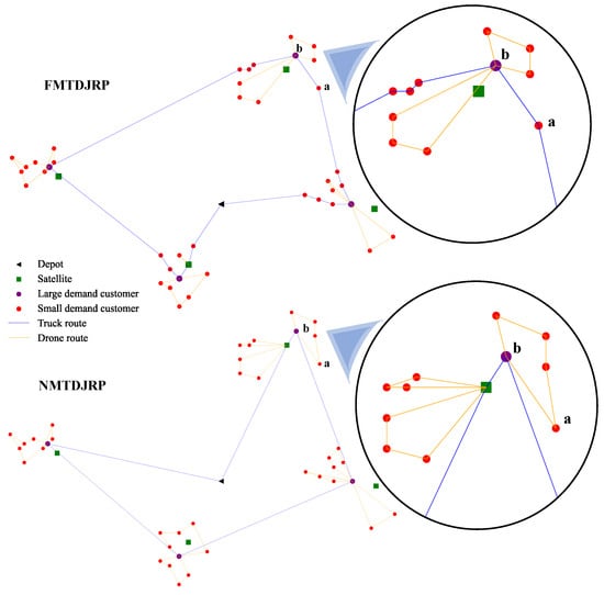
Figure 10. Comparison of optimal routes in the FMTDJRP and the NMTDJRP.

6. Conclusions

As a prominent pattern of truck–drone synchronization, the mothership system has recently attracted growing research interest. In this system, a truck sequentially visits designated rendezvous nodes, where a fleet of drones is launched and retrieved during the truck’s stops, enabling efficient service to nearby customers. In this paper, we investigate a flexible variant of the mothership system, referred to as the FMTDJRP. In the FMTDJRP, the truck is permitted to serve customers who (1) have demands exceeding the drones’ payload capacity, (2) are located in areas inaccessible to drones, or (3) can reduce the overall travel cost if served by the truck—factors that have been largely neglected in the existing mothership system-based models. The problem is formulated as a MILP model that aims to minimize the total travel cost while capturing the flexible allocation of customers between the truck and drone routes. Furthermore, an efficient ALNS metaheuristic is developed, augmented by a knowledge-based acceleration strategy to enhance computational performance. The proposed method demonstrates significant improvements in both execution time and solution quality, confirming its effectiveness for complex truck–drone coordination scenarios.

Extensive numerical experiments wer conducted to test the FMTDJRP in the context of diverse customer distribution scenarios and various drone feature combinations. Some characteristics of the FMTDJRP can be concluded here. In terms of cost saving, the FMTDJRP performs the best in the scenario in which customers are distributed in clusters. With a longer flight range and a larger load capacity of drones, the total cost for the scenario in which customers are distributed randomly drops significantly, whereas that for the clustering scenario stays almost unchanged. As for the flexibility, a comparison is conducted between the system with truck access to small-demand customers, namely the FMTDJRP, and the one without, namely the NMTDJRP. The results show that the NMTDJRP cannot always yield full solutions where all customers are served, while the FMTDJRP is able to adapt to diverse node distribution scenarios and yield more economic solutions. The adaptability brought by the flexibility makes the FMTDJRP not only a routing optimization model but also an assessment tool. Employing it in the decision-making stage, a logistics company is able to evaluate the necessity of using drones for delivery in an area and to give advice on the purchase of drones by estimating cost savings brought by different drone technological parameters.

The flexibility could be enhanced in several ways by future research. First, drones could be allowed to be retrieved at another rendezvous node instead of returning to the same rendezvous node as when they are launched. Second, the number of trucks could be increased. Thus, situations in which drones are launched by one truck and retrieved by another truck would be discussed. Moreover, the majority of papers assume that the truck travels an Euclidean distance between two locations. Taking the real road network structure into consideration would be more practical.

References

- Rose, C. Amazon’s Jeff Bezos Looks to the Future. 2013. Available online: https://www.cbsnews.com/news/amazons-jeff-bezos-looks-to-the-future/ (accessed on 30 October 2025).
- Koetsier, J. Google Now Owns the ‘Largest Residential Drone Delivery Service in the World’. Forbes, 25 August 2021. Available online: https://www.forbes.com/sites/johnkoetsier/2021/08/25/google-now-owns-the-largest-residential-drone-delivery-service-in-the-world/ (accessed on 30 October 2025).
- Zhou, R.; Lei, D.; Zhou, X. Multi-objective energy-efficient interval scheduling in hybrid flow shop using imperialist competitive algorithm. IEEE Access 2019, 7, 85029–85041. [Google Scholar] [CrossRef]
- Bian, J.; Huang, H.; Yu, Q.; Zhou, R. Search-to-Crash: Generating safety-critical scenarios from in-depth crash data for testing autonomous vehicles. Energy 2025, 332, 137174. [Google Scholar] [CrossRef]
- Min, K.; Sim, G.; Ahn, S.; Park, I.; Yoo, S.; Youn, J. Multi-Level Deceleration Planning Based on Reinforcement Learning Algorithm for Autonomous Regenerative Braking of EV. World Electr. Veh. J. 2019, 10, 57. [Google Scholar] [CrossRef]
- Xu, Y.; Liu, W. Enhanced A*–Fuzzy DWA Hybrid Algorithm for AGV Path Planning in Confined Spaces. World Electr. Veh. J. 2025, 16, 538. [Google Scholar] [CrossRef]
- Zhou, R.; Bian, J.; Liu, X.; Huang, H. Diffcrash: Leveraging Denoising Diffusion Probabilistic Models to Expand High-Risk Testing Scenarios Using In-Depth Crash Data. Expert Syst. Appl. 2025, 287, 128140. [Google Scholar] [CrossRef]
- Wolf, H. We’re About to See the Golden Age of Drone Delivery—Here’s Why. World Economic Forum, 6 July 2020. Available online: https://www.weforum.org/agenda/2020/07/golden-age-drone-delivery-covid-19-coronavirus-pandemic-technology/ (accessed on 30 October 2025).
- Rodrigues, T.A.; Patrikar, J.; Oliveira, N.L.; Matthews, H.S.; Scherer, S.; Samaras, C. Drone Flight Data Reveal Energy and Greenhouse Gas Emissions Savings for Very Small Package Delivery. Patterns 2022, 3, 100569. [Google Scholar] [CrossRef]
- Kukolj, G. Last Mile Delivery: Costs, Definition & How to Optimize. OptimoRoute, 26 May 2020. Available online: https://optimoroute.com/last-mile-delivery/ (accessed on 30 October 2025).
- Murray, C.C.; Chu, A.G. The flying sidekick traveling salesman problem: Optimization of drone-assisted parcel delivery. Transp. Res. Part C Emerg. Technol. 2015, 54, 86–109. [Google Scholar] [CrossRef]
- Karak, A.; Abdelghany, K. The hybrid vehicle-drone routing problem for pick-up and delivery services. Transp. Res. Part C Emerg. Technol. 2019, 102, 427–449. [Google Scholar] [CrossRef]
- Thornton, S.; Gallasch, G.E. Swarming logistics for tactical last-mile delivery. In Proceedings of the International Conference on Science and Innovation for Land Power (ICSILP 2018), Adelaide, SA, Australia, 5–6 September 2018; Defence Science and Technology Group: Edinburgh, SA, Australia, 2018. Available online: https://www.dst.defence.gov.au/sites/default/files/basic_pages/documents/ICSILP18_IntSes-Thornton_Gallasch-Swarming_Logistics_for_Last-Mile_Logistics.pdf (accessed on 30 October 2025).
- Goodchild, A.; Toy, J. Delivery by drone: An evaluation of unmanned aerial vehicle technology in reducing CO2 emissions in the delivery service industry. Transp. Res. Part D Transp. Environ. 2018, 61, 58–67. [Google Scholar] [CrossRef]
- Chao, I.-M. A tabu search method for the truck and trailer routing problem. Comput. Oper. Res. 2002, 29, 33–51. [Google Scholar] [CrossRef]
- Derigs, U.; Pullmann, M.; Vogel, U. Truck and trailer routing—Problems, heuristics and computational experience. Comput. Oper. Res. 2013, 40, 536–546. [Google Scholar] [CrossRef]
- Villegas, J.G.; Prins, C.; Prodhon, C.; Medaglia, A.L.; Velasco, N. GRASP/VND and multi-start evolutionary local search for the single truck and trailer routing problem with satellite depots. Eng. Appl. Artif. Intell. 2010, 23, 780–794. [Google Scholar] [CrossRef]
- Dellaert, N.; Van Woensel, T.; Crainic, T.G.; Saridarq, F.D. A multi-commodity two-Echelon capacitated vehicle routing problem with time windows: Model formulations and solution approach. Comput. Oper. Res. 2021, 127, 105154. [Google Scholar] [CrossRef]
- Li, H.; Liu, Y.; Jian, X.; Lu, Y. The two-echelon distribution system considering the real-time transshipment capacity varying. Transp. Res. Part B Methodol. 2018, 110, 239–260. [Google Scholar] [CrossRef]
- Zhou, L.; Baldacci, R.; Vigo, D.; Wang, X. A Multi-Depot Two-Echelon Vehicle Routing Problem with Delivery Options Arising in the Last Mile Distribution. Eur. J. Oper. Res. 2018, 265, 765–778. [Google Scholar] [CrossRef]
- Archetti, C.; Peirano, L.; Speranza, M.G. Optimization in multimodal freight transportation problems: A Survey. Eur. J. Oper. Res. 2022, 299, 1–20. [Google Scholar] [CrossRef]
- Es Yurek, E.; Ozmutlu, H.C. A decomposition-based iterative optimization algorithm for traveling salesman problem with drone. Transp. Res. Part C Emerg. Technol. 2018, 91, 249–262. [Google Scholar] [CrossRef]
- Ha, Q.M.; Deville, Y.; Pham, Q.D.; Hà, M.H. On the min-cost Traveling Salesman Problem with Drone. Transp. Res. Part C Emerg. Technol. 2018, 86, 597–621. [Google Scholar] [CrossRef]
- Murray, C.C.; Raj, R. The multiple flying sidekicks traveling salesman problem: Parcel delivery with multiple drones. Transp. Res. Part C Emerg. Technol. 2020, 110, 368–398. [Google Scholar] [CrossRef]
- Sacramento, D.; Pisinger, D.; Ropke, S. An adaptive large neighborhood search metaheuristic for the vehicle routing problem with drones. Transp. Res. Part C Emerg. Technol. 2019, 102, 289–315. [Google Scholar] [CrossRef]
- Schermer, D.; Moeini, M.; Wendt, O. A hybrid VNS/Tabu search algorithm for solving the vehicle routing problem with drones and en route operations. Comput. Oper. Res. 2019, 109, 134–158. [Google Scholar] [CrossRef]
- Salama, M.R.; Srinivas, S. Collaborative truck multi-drone routing and scheduling problem: Package delivery with flexible launch and recovery sites. Transp. Res. Part E Logist. Transp. Rev. 2022, 164, 102788. [Google Scholar] [CrossRef]
- Mahmoudi, B.; Eshghi, K. Energy-constrained multi-visit TSP with multiple drones considering non-customer rendezvous locations. Expert Syst. Appl. 2022, 210, 118479. [Google Scholar] [CrossRef]
- Sakharkar, A. A2Z Drone Delivery Unveils a Multi-Drop Dual-Payload Delivery Drone. Inceptive Mind. 2021. Available online: https://www.inceptivemind.com/a2z-drone-delivery-rdsx-multi-drop-dual-payload-delivery-drone/20842/ (accessed on 30 October 2025).
- Poikonen, S.; Golden, B. Multi-visit drone routing problem. Comput. Oper. Res. 2020, 113, 104802. [Google Scholar] [CrossRef]
- Salama, M.; Srinivas, S. Joint optimization of customer location clustering and drone-based routing for last-mile deliveries. Transp. Res. Part C Emerg. Technol. 2020, 114, 620–642. [Google Scholar] [CrossRef]
- Pisinger, D.; Ropke, S. Large Neighborhood Search. In Handbook of Metaheuristics; Gendreau, M., Potvin, J.-Y., Eds.; Springer: Boston, MA, USA, 2010; Volume 146, pp. 399–419. [Google Scholar] [CrossRef]
- Mara, S.T.W.; Norcahyo, R.; Jodiawan, P.; Lusiantoro, L.; Rifai, A.P. A survey of adaptive large neighborhood search algorithms and applications. Comput. Oper. Res. 2022, 146, 105903. [Google Scholar] [CrossRef]
- Ropke, S.; Pisinger, D. An Adaptive Large Neighborhood Search Heuristic for the Pickup and Delivery Problem with Time Windows. Transp. Sci. 2006, 40, 455–472. [Google Scholar] [CrossRef]
- Hemmelmayr, V.C.; Cordeau, J.-F.; Crainic, T.G. An adaptive large neighborhood search heuristic for Two-Echelon Vehicle Routing Problems arising in city logistics. Comput. Oper. Res. 2012, 39, 3215–3228. [Google Scholar] [CrossRef] [PubMed]
- Shaw, P. Using Constraint Programming and Local Search Methods to Solve Vehicle Routing Problems. In Principles and Practice of Constraint Programming—CP98; Maher, M., Puget, J.-F., Eds.; Springer: Berlin/Heidelberg, Germany, 1998; Volume 1520, pp. 417–431. [Google Scholar] [CrossRef]
- Demir, E.; Bektaş, T.; Laporte, G. An adaptive large neighborhood search heuristic for the Pollution-Routing Problem. Eur. J. Oper. Res. 2012, 223, 346–359. [Google Scholar] [CrossRef]
- Allain, R. Physics of the Amazon Octocopter Drone. Wired. 3 December 2013. Available online: https://www.wired.com/2013/12/physics-of-the-amazon-prime-air-drone/ (accessed on 30 October 2025).
Disclaimer/Publisher’s Note: The statements, opinions and data contained in all publications are solely those of the individual author(s) and contributor(s) and not of MDPI and/or the editor(s). MDPI and/or the editor(s) disclaim responsibility for any injury to people or property resulting from any ideas, methods, instructions or products referred to in the content. |
© 2025 by the authors. Published by MDPI on behalf of the World Electric Vehicle Association. Licensee MDPI, Basel, Switzerland. This article is an open access article distributed under the terms and conditions of the Creative Commons Attribution (CC BY) license (https://creativecommons.org/licenses/by/4.0/).