Automatic Longitudinal Regenerative Control of EVs Based on a Driver Characteristics-Oriented Deceleration Model

Abstract

To preserve the fun of driving and enhance driving convenience, a smart regenerative braking system (SRS) is developed. The SRS provides automatic regeneration that is appropriate for the driving conditions, but the existing technology has a low level of acceptability and comfort. To solve this problem, this paper presents an automatic regenerative control system based on a deceleration model that reflects the driver’s characteristics. The deceleration model is designed as a parametric model that mimics the driver’s behavior. In addition, it consists of parameters that represent the driver’s characteristics. These parameters are updated online by a learning algorithm. The validation results of the vehicle testing show that the vehicle maintained a safe distance from the leading car while simulating a driver’s behavior. Of all the deceleration that occurred during the testing, 92% was conducted by the automatic regeneration system. In addition, the results of the online learning algorithm are different based on the driver’s deceleration pattern. The presented automatic regenerative control system can be safely used in diverse car-following situations. Moreover, the system’s acceptability is improved by updating the driver characteristics. In the future, the algorithm will be extended for use in more diverse deceleration situations by using intelligent transportation system information.

1. Introduction

Various advanced driving assistance systems (ADASs) are being applied to production vehicles as vehicle control technology is improved and the prices of sensors continue to decrease. Advanced cruise control (ACC) is widely provided as a trim option by many original equipment manufacturer (OEM) companies such as Hyundai, Toyota, Volkswagen, etc. However, the fun of driving is decreased as ACC minimizes the driver’s control of the vehicle. Some drivers want to accelerate themselves even while ACC is operating, because most of the fun of driving comes from acceleration.

To satisfy both convenience and the fun of driving, a system of automatic regenerative control called the smart regenerative braking system (SRS) was developed [1]. The SRS generates adequate regeneration according to the specific car-following situation, which means the driver does not use the brake pedal. Therefore, it preserves the fun of driving while increasing the convenience. In addition, the vehicle’s energy efficiency can be improved by energy recovery from the automatic regenerative braking system.

The SRS is a type of intelligent braking system that controls regenerative braking according to the driving conditions. There have been various studies regarding intelligent braking systems. Lin et al. proposed an active regenerative control system that uses an energy boost mechanism to improve the braking performance [2]. In another paper [3], a fuzzy logic–based regenerative braking strategy that determines the distribution between the friction brake and regeneration was proposed to maximize the driving range of electric vehicles (EVs). In addition, another study [4] suggested an anti-disturbance controller to shorten the braking distance and time. While these papers had different objectives, they all presented an intelligent braking system.

However, the existing SRS applied in production vehicles has some limitations. First, it utilizes map-based control, which has only three discrete torque levels [1]. This can cause driver discomfort during level transitions [5,6]. Second, the deceleration profile of an SRS is different from human driving, generating heterogeneity [7,8,9]. Third, the SRS cannot stop the vehicle, so it is difficult to use in situations with heavy traffic.

Considering these limitations, the deceleration used in automatic regenerative braking should meet certain requirements. First, it is necessary to simulate human deceleration behavior and reflect driver characteristics in order to reduce the discomfort and heterogeneity of the system [10,11,12,13]. Second, the SRS should generate a smooth deceleration profile while maintaining a safe distance from the leading car. Third, it should be able to be applied in diverse car-following situations, including traffic jams, to extend its usability.

There have been various studies attempting to represent vehicle motion in car-following conditions. The intelligent driver model (IDM) is a representative parametric car-following model [14]. The parameters of the IDM reflect the driver’s driving characteristics, so it is possible to reflect each driver’s acceleration and deceleration patterns to some extent. However, it cannot mimic human deceleration because it does not consider reaction delay.

In addition to the parametric modeling method, artificial neural networks (ANNs) are actively used in car-following models. In [15], Khodayari et al. suggested a modified car-following model based on a neural network model that considers the human driver effect. Another study [16] showed that an ANN model developed using data of one driver has low accuracy when used by other drivers. The car-following model based on the ANN has strengths, in that it can mimic human behavior by learning the driving data and consider the nonlinear characteristics between multiple inputs and acceleration with little processing time. However, it is difficult to reflect driver characteristics online because the ANN model is trained with a huge amount of data, which requires a relatively long time.

To overcome the limitations of the existing SRS and previous studies, this paper suggests a method of automatic regenerative control based on a deceleration model that reflects driver characteristics. First, the state recognition algorithm was developed to recognize the necessity of automatic regenerative braking and determine the details of car-following situations. Second, a parametric deceleration model was designed with parameters that represent the driver’s deceleration pattern. Especially, the deceleration model was designed to mimic a human driver’s behavior when decelerating. Third, learning vectors were defined to manage the driver’s deceleration pattern and calculate the driver parameters. Last, an online learning algorithm was designed to update the learning vectors.

The rest of the paper is organized as follows. Section 2 describes the overall structure of the algorithm. Section 3 describes the state recognition algorithm, which recognizes the necessity of deceleration and its cause. In Section 4, the deceleration model, which consists of driver parameters, is explained. Section 5 describes the online learning algorithm, which updates the learning vector that represents the driver characteristics. Section 6 shows the validation results when the designed algorithm was applied to the test vehicle. Section 7 concludes the paper.

2. System Overview

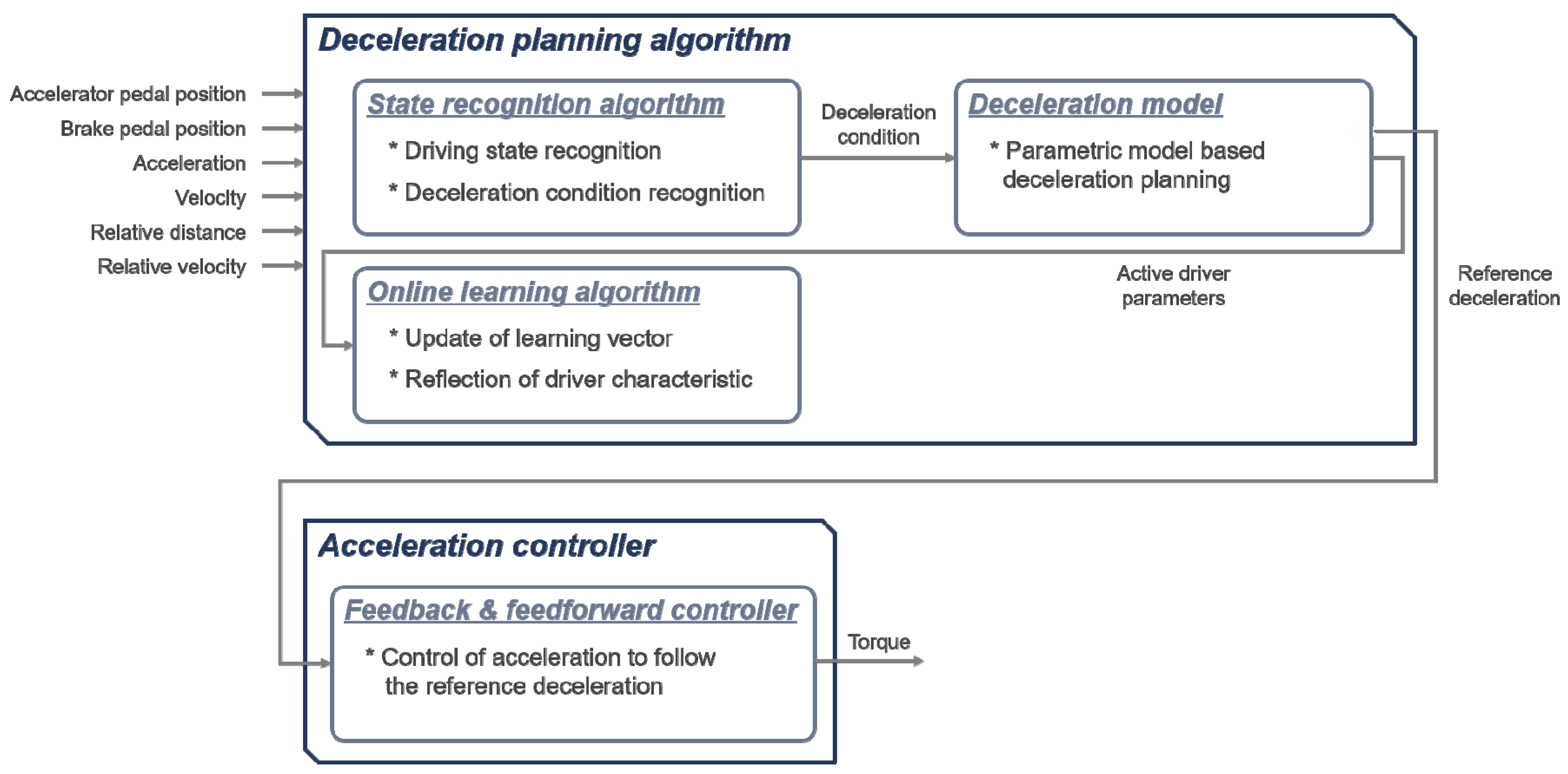
The system configuration of automatic regenerative control based on the proposed algorithm is shown in Figure 1. Automatic regenerative control is conducted by the deceleration planning algorithm and acceleration controller. The deceleration planning algorithm has the role of calculating the reference deceleration of the next time step, and the acceleration controller determines an adequate value of torque to follow the reference deceleration.

The deceleration planning algorithm contains three smaller algorithms: state recognition algorithm, deceleration model, and online learning algorithm. First, the state recognition algorithm recognizes the state of vehicle motion and determines the deceleration condition as either car-following, traffic jam, or cut-in. Second, the deceleration model calculates the reference deceleration using the designed parametric model. Third, the online learning algorithm updates the driver characteristics. The online learning algorithm only operates when the acceleration controller is not operating, because it compares the planning results and the driving data of the human driver. Lastly, the acceleration controller controls the vehicle to follow the reference deceleration calculated by the planning algorithm.

3. State Recognition Algorithm

In this section, the state recognition algorithm is proposed to highlight the necessity of the deceleration and determine the detailed situation of the car-following. For this purpose, the algorithm consists of two recognition algorithms: driving state and deceleration condition. Each algorithm was designed with the state flowchart and is described in Section 3.1 and Section 3.2 individually.

3.1. Driving State Recognition

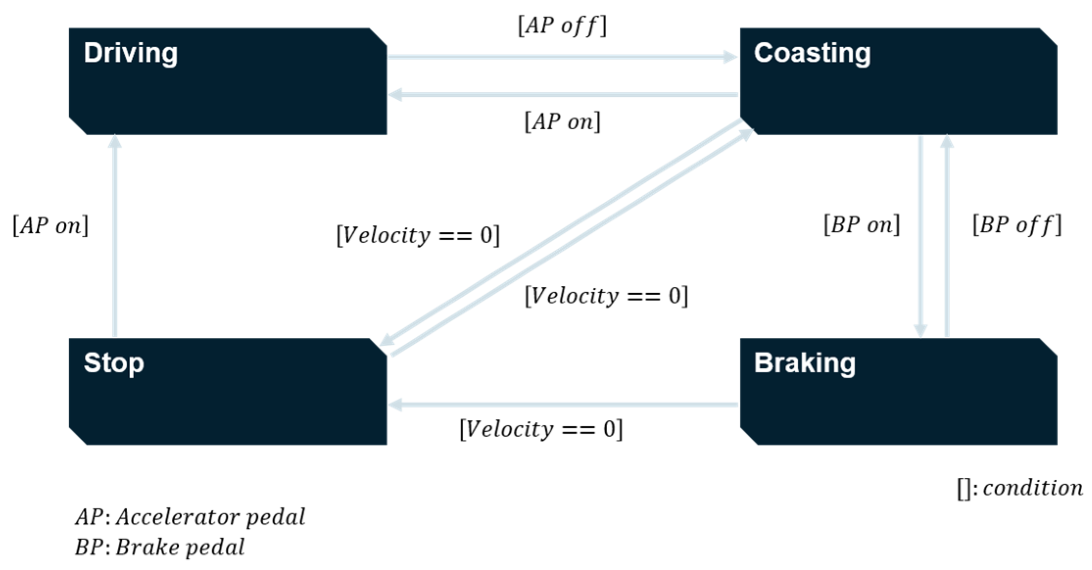
Automatic regenerative braking can operate only when the driver does not accelerate the vehicle. Therefore, driving condition was defined in order to monitor the vehicle’s motion based on the state of the accelerator and brake pedal. The driving condition includes four states: driving, coasting, braking, and stopping. Driving is when the driver pushes the accelerator pedal, so automatic regenerative control cannot operate. Coasting is when the driver does not push either the accelerator or the brake pedal, and the vehicle can be controlled by the automatic regenerative control. Braking is when the driver pushes the brake pedal. In this state, the deceleration model can generate the reference deceleration, but acceleration control is not possible. Stopping is when the vehicle speed is zero. Automatic regenerative control does not operate, because there is no need to decelerate in this state. The changes of driving state are shown in Figure 2. In addition, the operability of each algorithm and automatic regenerative control according to the driving conditions is shown in

Table 1. Operability of each algorithm according to the driving state.

Driving State	Deceleration Model	Online Learning Algorithm	Acceleration Control
Driving	X	X	X
Coasting	O	X	O
Decelerating	O	O	X
Stopping	X	X	X

O, possible; X, impossible.

. The online learning algorithm only operates when the driver decelerates the vehicle, because it needs the driving data.

3.2. Deceleration Condition Recognition

The deceleration model was designed to use different equations according to the vehicle speed, because keeping appropriate distance is crucial when the relative distance is small and vehicle speed is low. Therefore, the deceleration condition was defined to represent the current deceleration situation. The deceleration condition includes four states: none, car-following, traffic jam, and cut-in. None means deceleration because of the preceding car is not necessary. In this case, the deceleration planning algorithm does not calculate the reference deceleration. Car-following means deceleration because of the leading car when the vehicle speed is over 10 m/s. Traffic jam means deceleration by the preceding vehicle with a velocity under 10 m/s. Cut-in means deceleration is needed because a vehicle suddenly got into the same lane. It is recognized when the difference of relative distance between the previous and current time steps is more than 4 m, which is the usual overall vehicle length.

4. Parametric Deceleration Model

In this section, we propose a parametric deceleration model that is specialized for deceleration and has some driver parameters. First, the driving data acquired from the vehicle experiment were analyzed. Then, the deceleration profile was split into braking sections. Based on the braking sections, the driver parameters were defined, which are needed to generate a deceleration profile and represent the driver’s deceleration pattern. Using the driver parameters, the deceleration model was designed with different parametric equations according to the braking sections.

4.1. Split of Braking Section

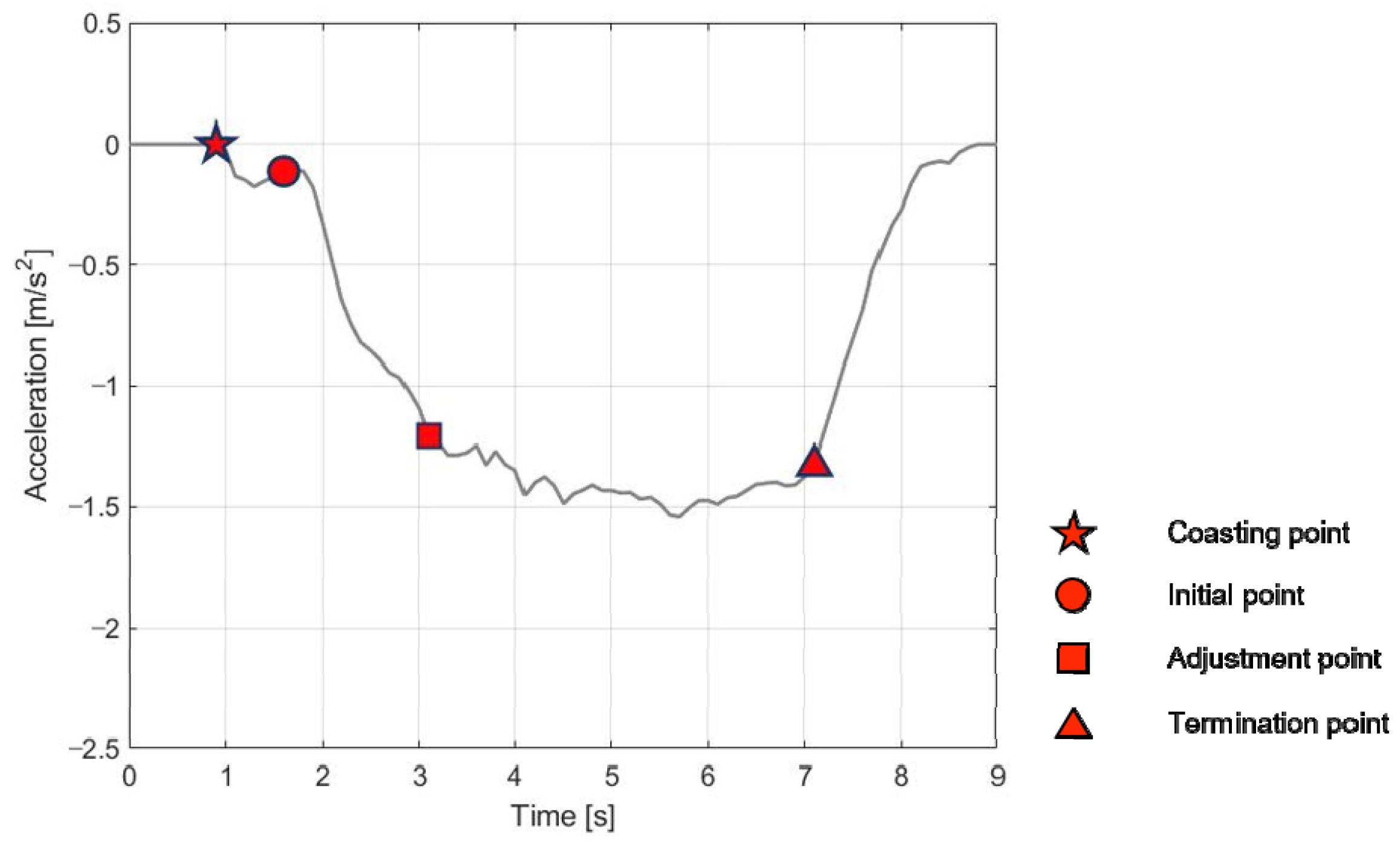
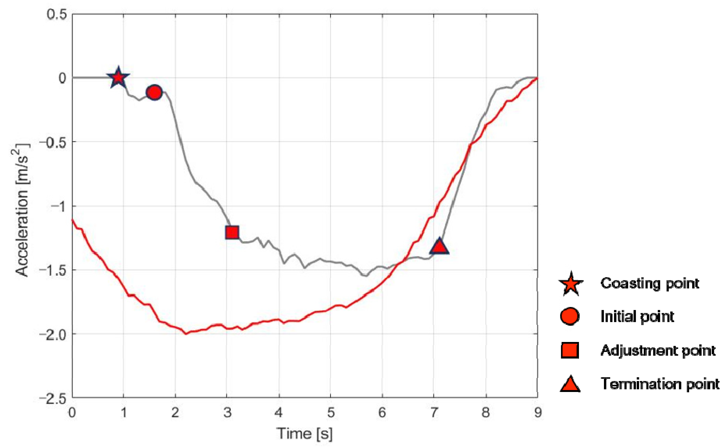
The general deceleration profiles in the car-following situation are shown in Figure 3. With the deceleration profile and pedal sensor data, the human driver’s behavior in the car-following condition can be divided into four steps:

• Release the accelerator pedal;
• Push the brake pedal to some extent with a similar ratio;
• Continuously push the brake pedal to keep a safe distance from the leading car;
• Gradually release the brake pedal.

With this procedure, the deceleration profile is split into four braking sections: coasting, initial, adjustment, and termination. Each braking point shown in Figure 3 represents the start of each braking section. The deceleration profile shown in Figure 3 was acquired through the vehicle test. The test driver drove a Hyundai Kona electric vehicle in a situation with a leading car. The deceleration profile is the sliced one when the ego vehicle decelerates to reduce its speed because of the preceding vehicle’s deceleration.

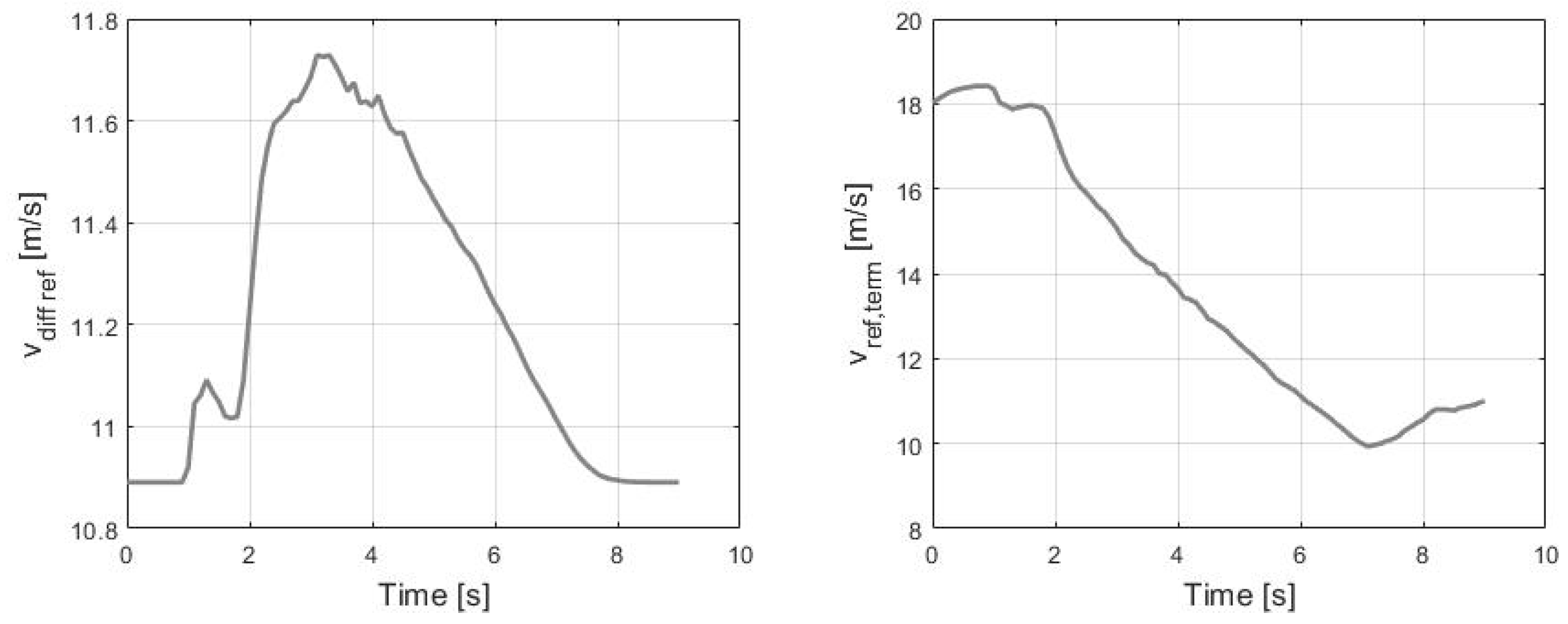
The coasting point refers to the time when the driver releases the accelerator pedal, so it is determined by the accelerator pedal sensor (APS) value. The initial point is the time when the driver pushes the brake pedal, which is found by the brake pedal sensor (BPS) value. After the initial point, the driver pushes the brake pedal with a similar ratio of acceleration. Then, the driver continuously pushes the brake pedal to maintain deceleration after the adjustment point. The adjustment point is determined as the time when $v_{diff\_ref}$, calculated by Equation (1), is maximum. The $v_{ref,adj}$ in Equation (1) is calculated with Equation (2), which is a modified equation of the basic intelligent driver model (IDM), a representative car-following model developed in 2000 by Treiber [14].

The basic equation of the IDM is shown in Equation (3), where $a_{\alpha }$, $v_{\alpha }$, and $s_{\alpha }$ represent acceleration, velocity, and relative distance of the ego vehicle; T is the minimum distance; $a_{max}$ is the maximum acceleration; $b$ is comfortable braking deceleration; $v_{rel}$ refers to relative velocity; and $v_0$ is the desired velocity on free roads. It represents the motion of the vehicle in a car-following situation with the velocity and distance term, which are the second and third terms in Equation (3). The velocity term means that the driver controls the vehicle speed considering $v_0$ on a free road where there is no leading car. The distance term refers to the driver controlling the relative distance adequately to maintain a safe distance. Its numerator can be considered as the desired distance in a car-following situation.

$$v_{diff\_ref}=v_{\alpha }-v_{ref,adj}$$

(1)

$$v_{ref,adj}=\frac{v_{\alpha }-v_{min}}{{\left(1-\frac{a_{\alpha }}{max\left(\left|a_{\alpha }\right|\right)}\right)}^{\frac{1}{4}}}$$

(2)

$$a_{\alpha }=a_{max}\left(1-{\left(\frac{v_{\alpha }}{v_0}\right)}^4-{\left(\frac{\left(s_0+v_{\alpha }T+\frac{v_{\alpha }{v}_{rel}}{2\sqrt{a_{max}b}}\right)}{s_{\alpha }}\right)}^2\right).$$

(3)

The termination point is determined as the point where $v_{ref,term}$, calculated by Equation (4), is minimum. It is also a modified version of basic IDM equation shown in Equation (3). Equations (2) and (4) were modified from the basic IDM equation to find the adjustment and termination points individually. They are the value of $v_0$ calculated from the IDM equation, which eliminates the distance term. The way of modifying the equation was found experimentally, and $v_{diff\_ref}$ and $v_{ref,term}$ are shown in Figure 4. As shown in Figure 4, $v_{diff\_ref}$ is maximized at the end of the initial section, and $v_{ref,term}$ is minimized at the end of the adjustment section.

$$v_{ref,term}=\frac{v_{\alpha }}{{\left(1-\frac{a_{\alpha }}{\max \left(\left|a_{\alpha }\right|\right)}\right)}^{\frac{1}{4}}}.$$

(4)

4.2. Driver Parameters

Based on the four braking sections, the deceleration model was designed. The deceleration model uses some parameters to generate the deceleration profile. These are the driver parameters, which are determined based on the car-following situation and the driver’s deceleration pattern. The types of driver parameters and their descriptions are shown in

Table 2. Types and descriptions of driver parameters.

Driver Parameter	Description
Initial distance ($s_{init})$	Relative distance at initial point
Adjustment distance ($s_{adj})$	Relative distance at adjustment point
Initial jerk (${\varphi }_{init})$	Slope of acceleration in initial section
Velocity difference ($v_{diff})$	Velocity difference with leading car speed at end of deceleration

. The four driver parameters described in Table 2 were selected because their values depend on both driving conditions and driver characteristics. Each driver parameter is explained in detail in the next part.

4.3. Deceleration Model Based on Braking Sections

The deceleration model was designed as different parametric equations according to the braking sections to reflect the features of the deceleration profile. In this part, the conditions of each section start and parametric equation are described. When the braking points in the driving data are determined (explained in Section 4.1), BPS, minimum velocity, and maximum absolute acceleration are used. In the deceleration model, however, BPS cannot be used because the driver does not push the brake pedal, and the minimum velocity and maximum absolute acceleration cannot be known until the deceleration ends. Therefore, a new algorithm to find each braking point was designed. Then, the deceleration model was designed depending on the braking section.

4.3.1. Coasting Section

In the coasting section, neither the accelerator nor the brake pedal is pushed, so deceleration stays at a very small value. To mimic the shape of deceleration in the coasting section, the deceleration model in the coasting section is designed as a constant function, as shown in Equation (5). In Equation (5), $a_{coast}$ means coasting acceleration, and its value was determined as the average value of acceleration in the coasting section from the vehicle experimental data.

$$a\left(k\right)=a_{coast}.$$

(5)

4.3.2. Initial Section

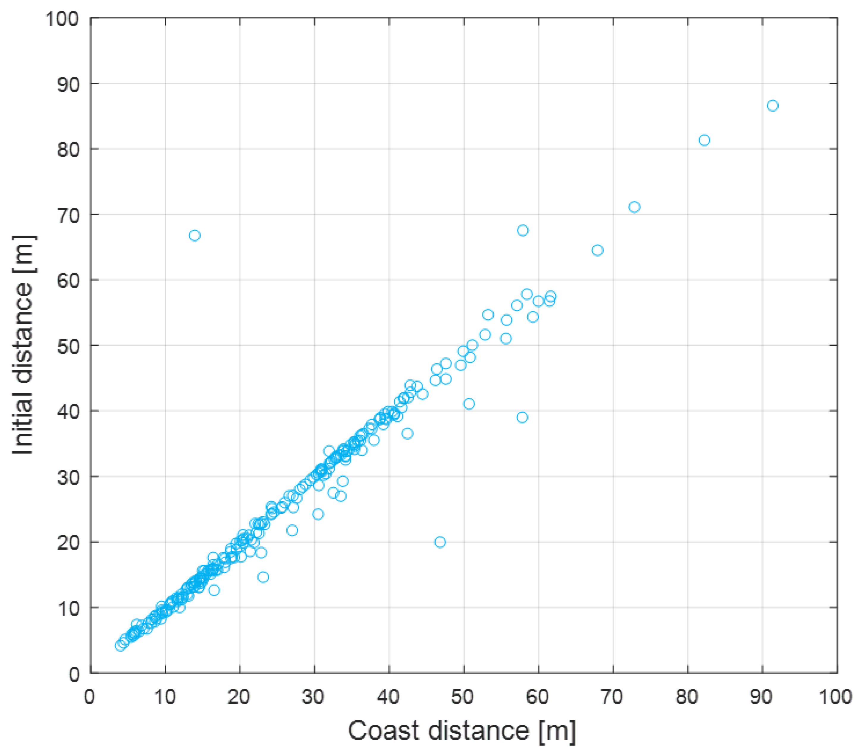
Unlike when the driver decelerates, the brake pedal is not used when SRS is in operation. Therefore, the relative distance was used to find the start of the initial section. The initial distance is calculated by the coasting distance based on their correlation, which is shown in Figure 5. The details of its calculation are described in Section 5.

In the initial section, the driver pushes the brake pedal with a similar ratio of acceleration. Therefore, the slope of acceleration is in a similar range, as shown in Figure 3. Because of the features in the initial section, the parametric equation was designed as a first-degree polynomial function, as shown in Equation (6), where ${\varphi }_{init}$ is the initial jerk and $T_s$ is the sampling rate of the deceleration model. The initial jerk depends on the car-following conditions, so its value is large when the leading car gets close very quickly or the relative distance is small. In addition, it is determined based on the driver’s characteristics, which is explained in Section 5.

$$a\left(k\right)=a\left(k-1\right)+{\varphi }_{init}{T}_s.$$

(6)

4.3.3. Adjustment Section

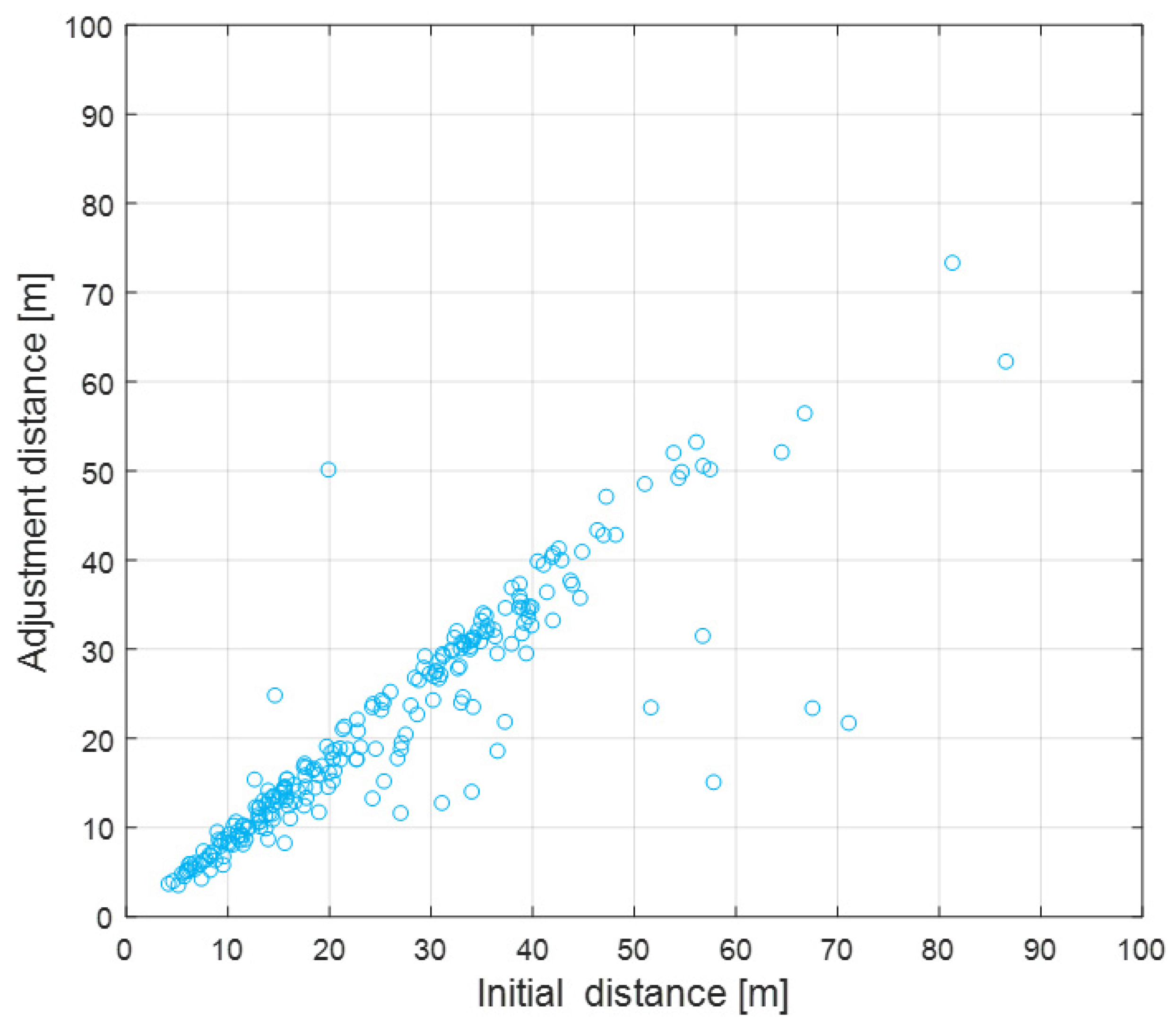
Similar to determining the start point of the initial section, the start of the adjustment section is set using the relative distance. The adjustment distance is highly correlated with the initial distance as shown in Figure 6. Therefore, the adjustment distance is calculated using the initial distance, and the adjustment section starts when the relative distance reaches the adjustment distance.

In the adjustment section, the driver continuously pushes the brake pedal to keep a safe distance. To simulate the driver’s behavior in the adjustment section, the deceleration model needs the reference value to follow. To find the appropriate equation to be used as reference acceleration, the constant acceleration (CA) model, which is widely used in speed trajectory prediction, was used [17,18,19,20,21]. The CA model is a parametric equation to calculate the acceleration in order to reach a desirable velocity at a specific location, as shown in Equation (7), where $v_2$ is the desirable velocity, $v_1$ is the current vehicle speed, and $d$ is the distance to the specific location.

$$a_{CA}=\frac{v_2^2-v_1^2}{2d}.$$

(7)

Most drivers tend to decelerate to follow the leading vehicle’s speed in car-following situations. However, some people decelerate more than the leading car speed, and others decelerate less. To reflect this type of deceleration pattern, Equation (7) was modified as Equation (8), which replaces $v_2$ as $v_2-v_{diff}$, so it can consider different deceleration patterns. For example, if $v_{diff}$ is 1 m/s, it means the driver has a tendency to decelerate 1 m/s less than the leading vehicle.

$$a_{CA}=\frac{{\left(v_2-v_{diff}\right)}^2-v_1^2}{2d}.$$

(8)

Figure 7 shows the measured deceleration from the vehicle experiment and the modified CA model when the desirable velocity is the leading vehicle speed and d is the relative distance. In the adjustment section, the deceleration slowly follows the CA model.

However, in traffic jam situations, where the relative distance is small and vehicle speed is low, the value calculated by the CA model is not enough to maintain a safe distance from the preceding car. Therefore, the constant time gap (CTG) policy was added to calculate the reference acceleration in these situations [22,23,24,25,26]. The acceleration for CTG is calculated with Equations (9)–(12), where $s_{min}$ is the minimum relative distance, $l_{i-1}$ is the length of the preceding car, $x_i$ and $x_{i-1}$ are the positions of the ego and leading cars, and $t_{ttc}$ and $\mathsf{\lambda }$ are control parameters.

$$L_{des}=s_{min}+t_{ttc}{\dot{x}}_i$$

(9)

$${ϵ}_i=x_i-x_{i-1}+l_{i-1}$$

(10)

$${\delta }_i={ϵ}_i+t_{ttc}{\dot{x}}_i$$

(11)

$$a_{CTG}=-\frac{1}{t_{ttc}}\left({\dot{ϵ}}_i+\lambda {\delta }_i\right).$$

(12)

If the equation for reference acceleration is converted to CTG policy discretely, the level transition of reference acceleration can be generated. To prevent the level transition, the equation of reference acceleration is designed to mix the weighted values of the CA model and CTG, as shown in Equation (13). The value of $w_{CA}$ is 1 when the velocity is 10 m/s and becomes smaller as the velocity decreases. The value of $w_{CTG}$ is 0 when the vehicle speed is 10 m/s and increases as the velocity decreases.

$$a_{ref}=\{\begin{array}{c}{a}_{CA} (v>10 \mathrm{m}/\mathrm{s})\\ w_{CA}{a}_{CA}+w_{CTG}{a}_{CTG} (v<10 \mathrm{m}/\mathrm{s})\end{array}.$$

(13)

To represent the pattern that deceleration follows the reference acceleration, the parametric equation was designed as Equation (14). As a result, deceleration follows the reference acceleration by I-control with the gain $k_{adj}$. The gain is set as a small value to simulate slow follow-up.

$$a\left(k\right)=a\left(k-1\right)+k_{adj}{{\displaystyle \sum }}_{i=adj}^{k-1}\left(a_{ref}\left(i\right)-a\left(i\right)\right)T_s.$$

(14)

4.3.4. Termination Section

As shown in Figure 7, deceleration follows the reference acceleration strongly after the two values meet at a specific point. Therefore, the point where the two values intersect was defined as the termination point. In the termination section, the same parametric equation was used as the equation of the adjustment section, as shown in Equation (15), but the gain was determined as a larger value than the adjustment section to represent fast follow-up.

$$a\left(k\right)=a\left(k-1\right)+k_{term}{{\displaystyle \sum }}_{i=term}^{k-1}\left(a_{ref}\left(i\right)-a\left(i\right)\right)T_s.$$

(15)

5. Online Learning Algorithm

In this section, the learning vectors are defined to manage the driver characteristics effectively. In addition, the learning vectors are updated online by the online learning algorithm, which changes their values by comparing the values of parameters from driving data and planning results. The online learning algorithm operates when the driver finishes decelerating. The designed algorithm reflects the driver characteristics with the learning vector, which has only eight values, so it is computationally light and suitable to implement in the vehicle.

5.1. Learning Vectors

5.1.1. Driver Parameters and Correlated Indices

The four driver parameters, whose values change according to the car-following situation and driver characteristics, are defined in Section 4. Among them, the initial jerk is used in explaining the overall online learning algorithm. As mentioned in Section 4.2, the values of driver parameters are dependent on the driving situation, so they were matched to the correlated indices that represent the driving situation, as shown in

Table 3. Driver parameters and correlated indices.

Driver Parameter	Correlated Index
Initial distance ($s_{init})$	Coasting distance
Adjustment distance ($s_{adj})$	Initial distance
Initial jerk (${\varphi }_{init})$	Initial index
Velocity difference ($v_{diff})$	Initial index

.

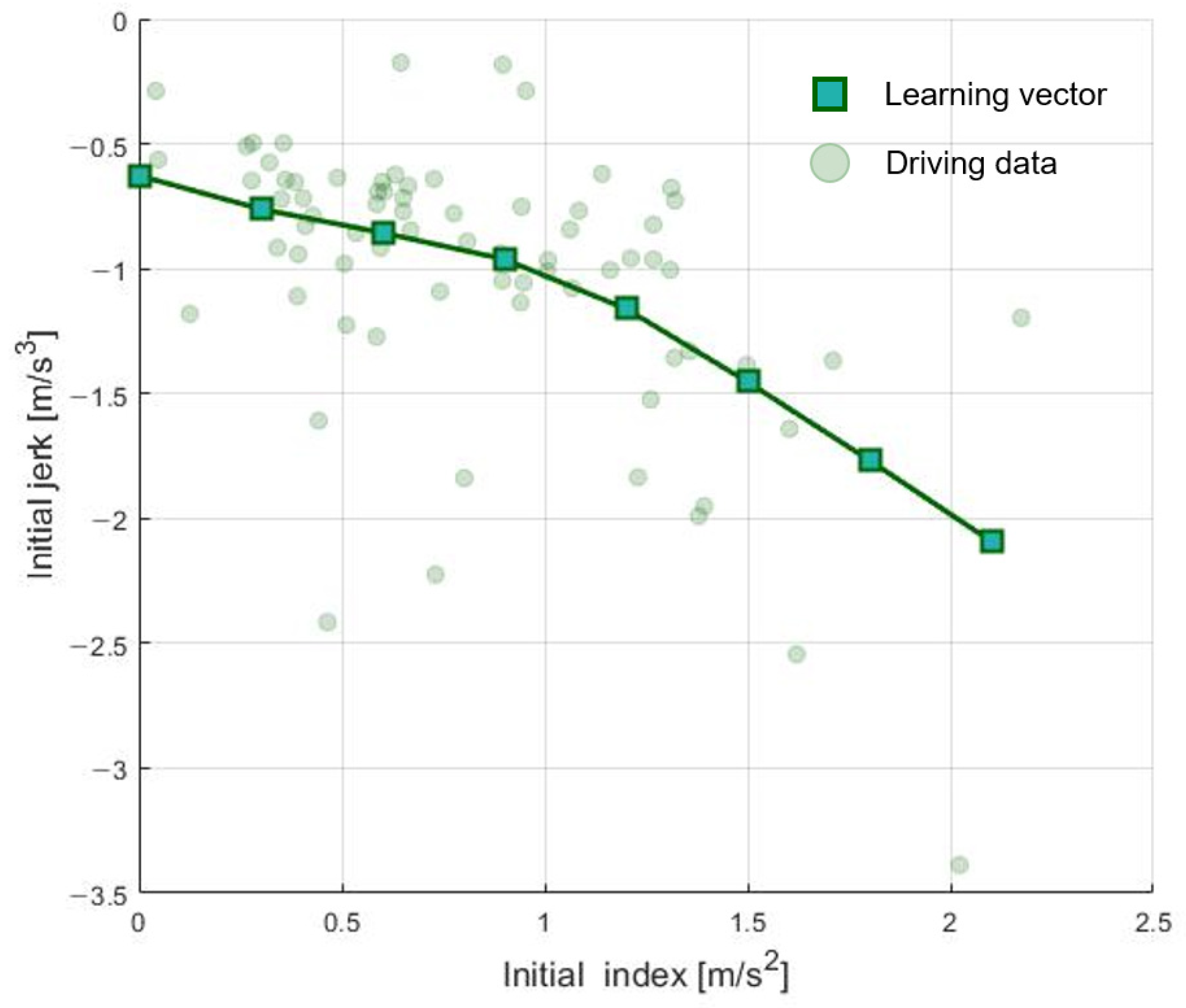
The initial jerk is correlated with the initial index. The initial index means the difference between deceleration and reference acceleration, which is mentioned in Section 4.3.3. As shown in Figure 8, the bigger the value of the initial index, the bigger the absolute value of the initial jerk. Although the correlation of the initial jerk’s absolute value and the initial index is proportional, it differs depending on the driver. For example, driver 3 has a smaller absolute value than driver 2 in the same initial index, which means that driver 2 is a moderate driver.

5.1.2. Learning and Effective Probability Vectors

To manage the different correlations of driver parameters and correlated indices depending on the driver, the learning vector was defined. It has eight values of driver parameters according to the predetermined index vector, as shown in Equations (16) and (17), where $V_{\theta }$ is the learning vector and $V_{\theta }\left(i\right)$ is ith element of the learning vector. Figure 9 shows an example of the learning vector after being updated by the online learning algorithm. The index vector is fixed as eight values considering the range of each index’s value. An example of the learning vector for the initial jerk is shown in

Table 4. Example of learning vector for initial jerk.

Index Number	1	2	3	4	5	6	7	8
Initial index $\left(\mathrm{m}/{\mathrm{s}}^2\right)$	0	0.3	0.6	0.9	1.2	1.5	1.8	2.1
Learning vector for initial jerk $\left(\mathrm{m}/{\mathrm{s}}^3\right)$	−0.6	−0.76	−0.86	−0.96	−1.16	−1.45	−1.77	−2.09

, representing the value of the initial jerk according to each initial index’s value. The basic learning vector was defined based on the average value of the driver parameters, then it is updated by the online learning algorithm, which is illustrated in the next part.

$$V_{\theta }=\left[P_{drv,1}, P_{drv,2},\cdots , P_{drv,7}, P_{drv,8}\right]$$

(16)

$$V_{\theta }\left(i\right)=P_{drv,i}, i\in \left\{1,2,\cdots ,7,8\right\}.$$

(17)

The major role of the learning vector is managing driver characteristics, but there is also one more important thing that it performs. The values of driver parameters used in the deceleration model are calculated based on the learning vector. The learning vector only has eight values of driver parameters according to the predetermined eight values of the correlated indices. Therefore, it is impossible to calculate the values of the driver parameters with only a single index value and the learning vector.

To solve this problem, the effective probability vector was defined. It has eight values for how much each value is used in calculating the driver parameters. The procedure of calculating the effective probability vector of the initial index is described as follows:

• Calculate the initial index from the driving data;
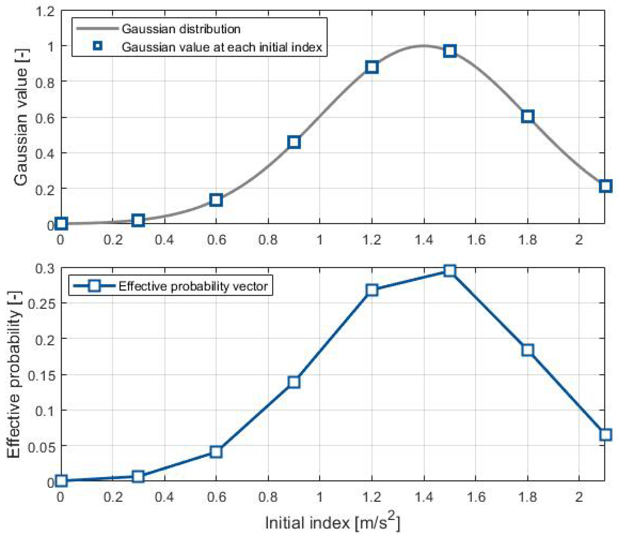
• Generate the Gaussian distribution, which has the mean value of the initial index calculated at step 1, as shown in Figure 10, using Equation (18), where $a$ is the value and $\sigma$ is the standard deviation of the initial index;

  $$f_g\left(x\right)=\frac{1}{\sqrt{2\pi {\sigma }^2}}{e}^{-\frac{{\left(x-a\right)}^2}{2{\sigma }^2}}.$$

  (18)
• Extract each value matching to the predetermined vector of the initial index, which is shown as blue squares in Figure 10;
• Normalize the eight values extracted in step 3 to make the sum of the eight values equal to 1, as shown in Equation (19), where $Idx\left(i\right)$ is the i-th value of the index vectors shown in Table 4.

  $$P_{eff}\left(i\right)=Norm\left(\frac{1}{\sqrt{2\pi {\sigma }^2}}{e}^{-\frac{{\left(Idx\left(i\right)-a\right)}^2}{2{\sigma }^2}}\right).$$

  (19)

After the procedure described above, the effective probability vector of the initial index that has eight values can be acquired. Effective probability vectors of the other correlated indices are calculated with the same procedure.

5.1.3. Calculation of the Driver Parameters

As mentioned in Section 4, the driver parameters are used in the deceleration model, so these values should be pre-calculated to generate the reference deceleration. To calculate the driver parameters, the learning and effective probability vectors are used. As mentioned in the previous part, the learning vector contains the eight values of the driver parameters according to the predetermined value of the correlated index. In addition, the effective probability vector has eight values of probability according to the predetermined value of the correlated index. If an element has high values in the effective probability vector, that means the deceleration situation is close to the predetermined value of the correlated index matched to the element. Therefore, the driver parameters are calculated by dot production of the learning and effective probability vectors, as shown in Equation (20), where ${\theta }_{act}$ is the driver parameter calculated by the equation and $V_{\theta }$ is the learning vector.

$${\theta }_{act}=P_{eff}·V_{\theta }.$$

(20)

5.2. Online Update of Learning Vectors

In the deceleration model, the driver parameters are calculated by the dot product of the learning and effective probability vectors, as described in Section 5.1.3. When the driver decelerates the vehicle not by using the SRS but by pushing the brake pedal, the driver parameters can also be calculated from the driving data. To avoid confusing these two values, driver parameters calculated by the two vectors were defined as active parameters, and those calculated from the driving data were defined as reference parameters.

If the learning vector does not reflect the driver characteristics perfectly, the values of the active and reference parameters are not the same. Therefore, to reflect the driver characteristics, the learning vectors have to be updated. The online learning algorithm that updates the learning vector consists of two steps. First, the target value, which indicates how much the learning vector is updated overall, is calculated by Equation (21), where ${\delta }_{\theta }$ is the target value, $\alpha$ is the learning rate, and ${\theta }_{ref}$ and ${\theta }_{act}$ refer to the reference and active parameters, respectively. The learning rate $\alpha$ was determined as the adequate value differently by the developer according to the types of learning vector. The learning rate values are shown in

Table 5. Values of learning rate according to the driver parameters.

Type of Learning Vector	Initial Distance	Adjustment Distance	Initial Jerk	Velocity Difference
Learning rate	0.1	0.1	0.2	0.1

. Then, the learning vector is updated with Equation (22) using the target value. In Equation (22), $\psi \left(i\right)$ is the learning degree, which is how much each element of the learning vector is updated. It is calculated by Equation (23) to update an element that has a bigger value of more effective probability. The entire procedure of online updating is employed whenever the driver finishes decelerating in a car-following situation.

$${\delta }_{\theta }=\alpha \left({\theta }_{ref}-{\theta }_{act}\right)$$

(21)

$$V_{\theta }\left(i\right)=V_{\theta }\left(i\right)+\psi \left(i\right){\delta }_{\theta }$$

(22)

$$\psi \left(i\right)={\left({\displaystyle \sum }{P}_{eff}\left(~i\right)\ast {\displaystyle \sum }\left(\frac{P_{eff}\left(i\right)}{P_{eff}\left(~i\right)}\right)\right)}^{-1}$$

(23)

$${\displaystyle \sum }{P}_{eff}\left(~1\right)=P_{eff}\left(2\right)+P_{eff}\left(3\right)+\dots +P_{eff}\left(8\right).$$

(24)

The learning vector updated by the online learning algorithm should converge when the same situation is repeated, where the values of the correlated index and the reference parameter are the same. The learning vector of the kth learning iteration is calculated by Equation (25). Likewise, the learning vector of the (k–1)th learning iteration is calculated by Equation (26). The change of the learning vector is defined as Equation (27). For the learning vector to converge, $E_k\left(i\right)$ should go to zero when the learning is repeated sufficiently. For this, the absolute proportion of $E_k\left(i\right)$ to $E_{k-1}\left(i\right)$ shown in Equation (28) should be smaller than 1.

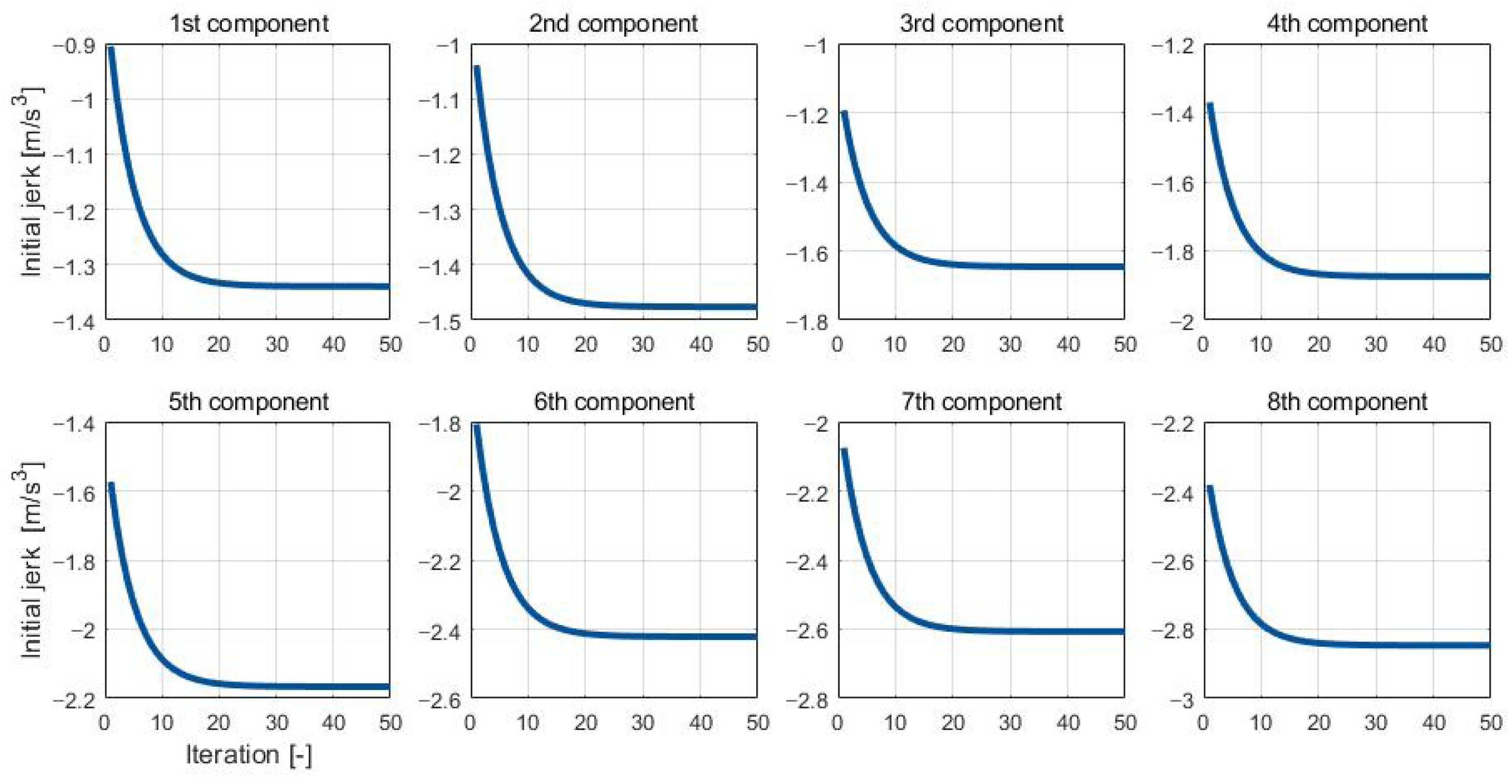
To satisfy the criteria shown in Equation (28), the learning rate should be in a specific range. When the learning rate is set as 2, the proportion of $E_k\left(i\right) \mathrm{to} E_{k-1}\left(i\right)$ is −1. In this case, each component of the learning vector is oscillated. Therefore, to guarantee convergence, the learning rate should be smaller than 2. The learning rate was determined according to its parametric characteristics, as shown in Table 5. For example, the rate for the initial jerk is larger than the rate for the other learning vectors. This is because the difference of the value depending on the driver is larger in the initial jerk than the other learning vectors. The learning vectors converge in about 20 iterations when the learning rate is 0.2 and about 40 when the learning rate is 0.1. The convergence of components of the learning vector for the initial jerk when the learning rate is 0.2 is shown in Figure 11.

$$V_{\theta ,k}\left(i\right)=V_{\theta ,k-1}\left(i\right)+\psi \left(i\right)\alpha \left({\theta }_{ref}-{\theta }_{act,k}\right)$$

(25)

$$V_{\theta ,k-1}\left(i\right)=V_{\theta ,k-2}\left(i\right)+\psi \left(i\right)\alpha \left({\theta }_{ref}-{\theta }_{act,k-1}\right)$$

(26)

$$E_k\left(i\right)=V_{\theta ,k}\left(i\right)-V_{\theta ,k-1}\left(i\right)$$

(27)

$$\left|\frac{E_k\left(i\right)}{E_{k-1}\left(i\right)}\right|=\left|\frac{{\theta }_{ref}-{\theta }_{act,k}}{{\theta }_{ref}-{\theta }_{act,k-1}}\right|<1$$

(28)

An example of online updating of the learning vector for the initial jerk is as follows. The learning vector of the initial jerk before update is shown as a green line in Figure 12. When the driver finishes decelerating in a car-following situation, the algorithm calculates the values of the initial index and the reference parameter of the initial jerk from the driving data; in this example, the values are $1.91\mathrm{m}/{\mathrm{s}}^2$ and $-2.72\mathrm{m}/{\mathrm{s}}^3$, respectively, shown as the red dot in Figure 12. Then, the algorithm calculates the effective probability vector using Equation (19) based on the value of the initial index. Next, the active parameter of the initial jerk is calculated with the learning and effective probability vectors. In this case, the calculated active parameter value is $-2.07\mathrm{m}/{\mathrm{s}}^3$. Using the values of the reference and active parameters, the target value is determined by Equation (21), which is $-0.13\mathrm{m}/{\mathrm{s}}^3$. Then, the learning degree is calculated using the initial index value to update the learning vector. Its value when the initial index is $1.91\mathrm{m}/{\mathrm{s}}^3$ is shown in

Table 6. Example of learning vectors for initial jerk.

Index Number	1	2	3	4	5	6	7	8
Initial index	0	0.3	0.6	0.9	1.2	1.5	1.8	2.1
Learning degree	0.70	0.70	0.70	0.70	0.76	0.89	1.09	1.05
Learning vector before update ($\mathrm{m}/{\mathrm{s}}^3$)	−0.91	−1.04	−1.19	−1.37	−1.57	−1.80	−2.08	−2.38
Learning vector after update ($\mathrm{m}/{\mathrm{s}}^3$)	−0.99	−1.13	−1.28	−1.46	−1.67	−1.92	−2.22	−2.52

. The value of the learning degree close to the value of the initial index is high. The last step is to update the learning vector using the target value and the learning degree based on Equation (22). The result of the updated learning vector is shown as a yellow line in Figure 12, and the values of the learning vector before and after the online update are shown in Table 6.

The online learning algorithm is summarized as follows; it operates whenever the driver is finished decelerating:

• Calculate the effective probability vector using the value of the correlated index;
• Calculate the active parameter by the dot product of the effective probability and learning vectors;
• Calculate the reference parameter from the driving data;
• Update the learning vector based on the active and reference parameters.

6. Validation

6.1. Acceleration Controller

For the vehicle to follow the reference deceleration, the acceleration controller is necessary. The acceleration controller was designed as a feedforward and feedback controller, as shown in Figure 13. The feedforward controller determines adequate torque based on a predefined equation according to the vehicle speed and reference deceleration, and the feedback controller calculates the value of torque using a proportional-integral (PI) controller. Then, the sum of these two values is sent to the vehicle control unit (VCU) through the controller area network (CAN).

6.2. Test Vehicle Configuration

For the algorithm validation, a Hyundai Kona electric vehicle was used. It is equipped with the radar sensor described in

Table 7. Specifications of radar sensor.

Index	Value
Maximum range	150 m
Field of view (FOV)	+/−10° over 60 m
	+/−45° under 60 m
Update rate	50 ms

. The designed algorithm was implemented on the target board, MPC 5674F of NXP semiconductors, specs of which are shown in

Table 8. Specifications of the central processing unit (CPU), random access memory (RAM), and flash memory of MPC5674F.

Component	Specification
CPU	Power architecture 200z7 core 265 MHz
RAM	256 KB data RAM with error correcting codes (ECC)
Flash	4 MB flash memory with ECC

. It acquires data such as velocity, relative distance, and relative velocity through the CAN communication. The torque calculated by the algorithm is sent to the VCU of the vehicle through CAN. In MPC 5674F, the deceleration planning algorithm is conducted every 100 ms and the acceleration control is performed every 10 ms.

6.3. Vehicle Test Environment

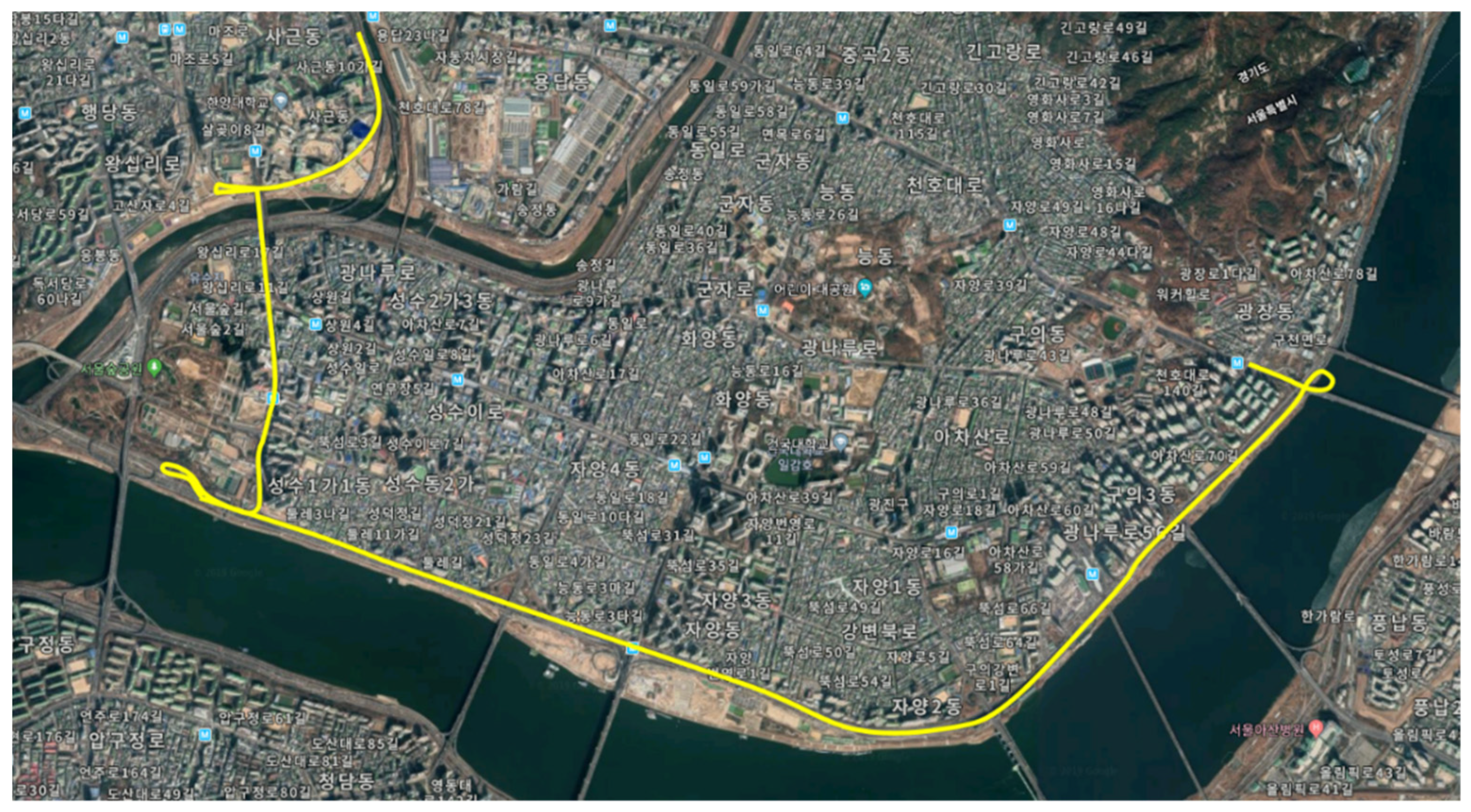
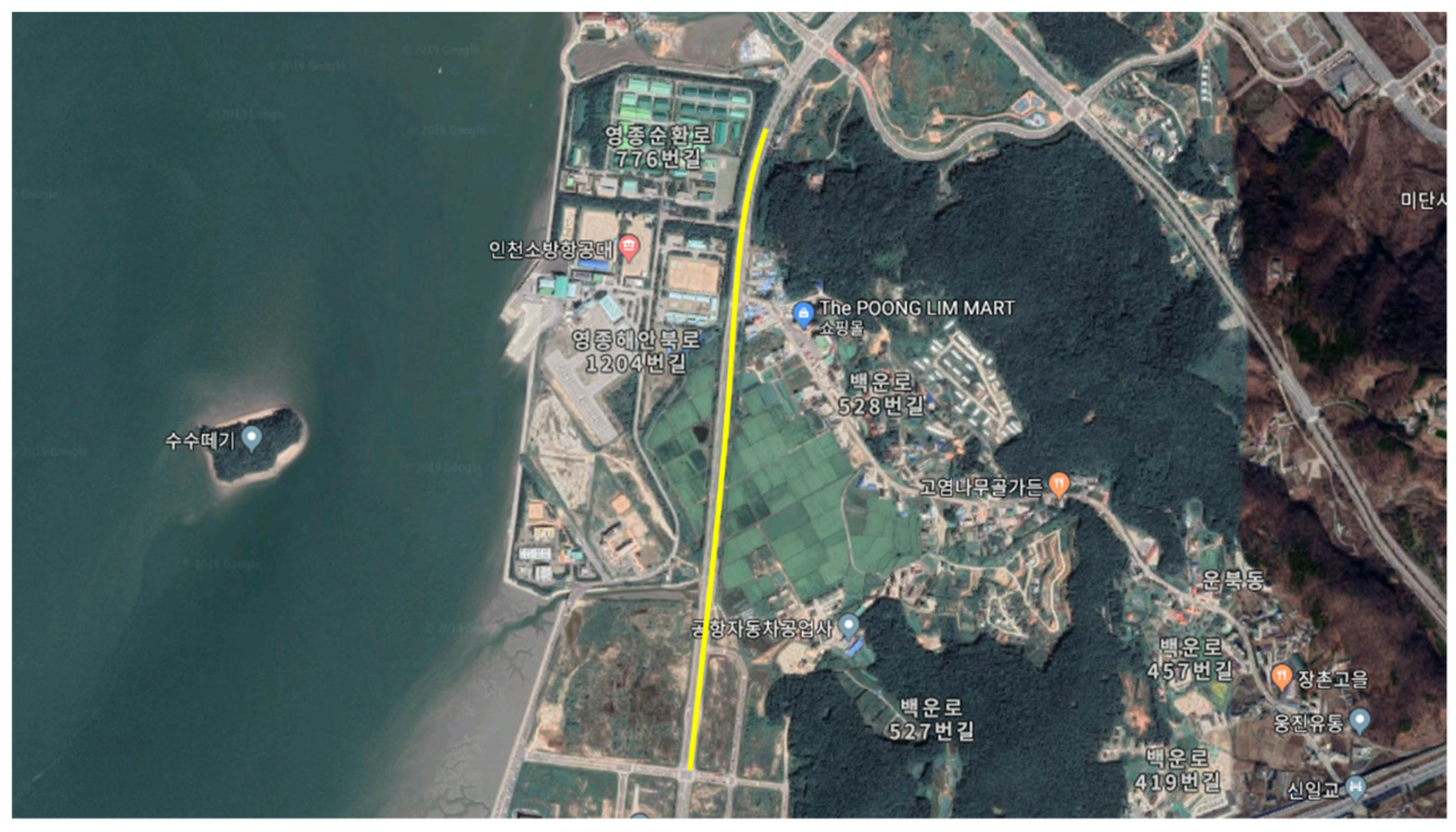
To validate the operation of automatic regenerative braking in general urban driving situations, a test driver drove the vehicle for about an hour on a specific route in Seoul, Korea, as shown in Figure 14. It includes urban roads where the speed limit is 50 km/h, but also highway where the maximum speed range is from 90 km/h to 110 km/h. In addition, there was a traffic jam on the highway, because the test time was 15:00, when there are many vehicles on the road. In conclusion, the test route contains both urban and highway situations, so that it is suitable to validate the algorithm in diverse car-following situations.

In most of the car-following situations, the test driver did not push the brake pedal and used the automatic regenerative braking. The brake pedal was used in other deceleration situations besides car-following such as speed humps, curves, and merges where there was no preceding vehicle.

6.4. Vehicle Test Results

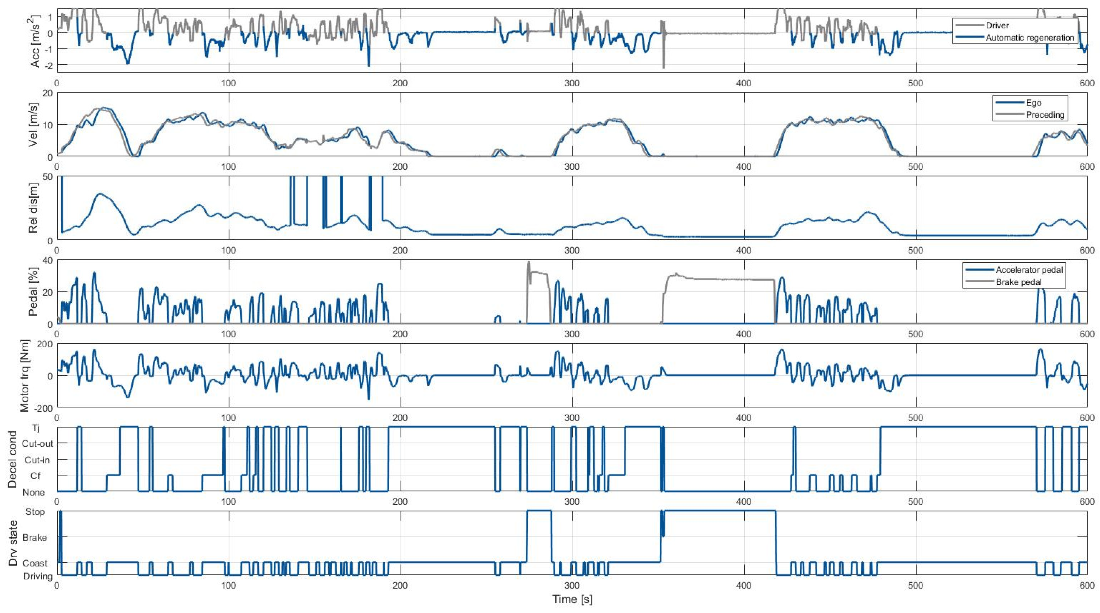
The test results have a time length of 50 min, and the divided test results on urban roads are shown in Figure 15. The first subplot of Figure 14 shows the measured acceleration. The range where automatic regeneration was operated is in blue. The third subplot of Figure 15 shows the positions of the pedals. The driver pushed the brake pedal only twice to keep the vehicle stopped, as shown by the gray line of the third graph. Except for these two braking situations, all deceleration was conducted by automatic regeneration.

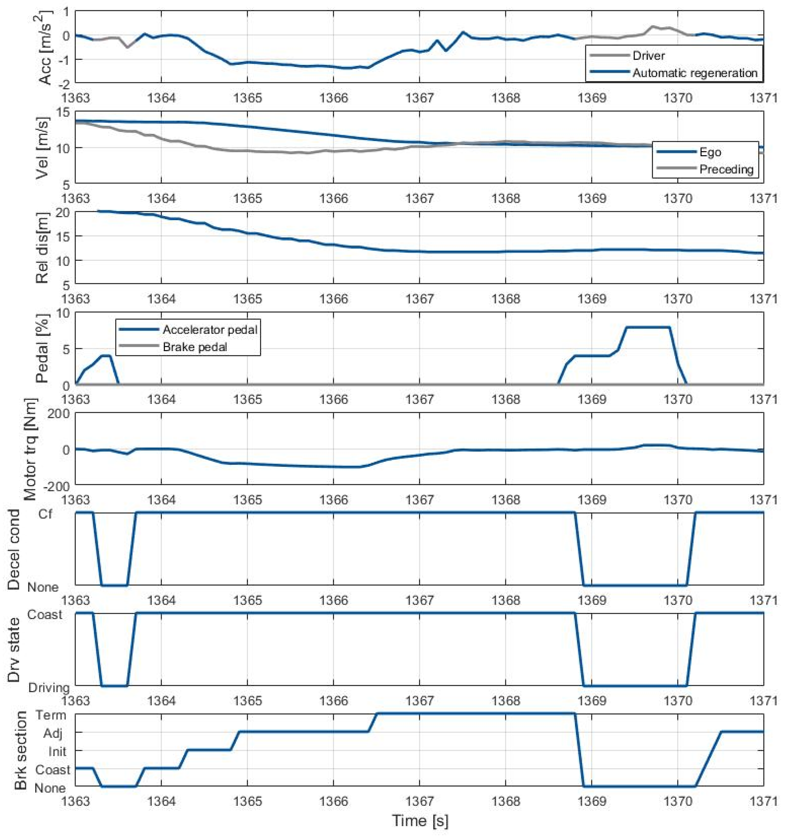
Figure 16 shows a deceleration profile where automatic regenerative braking operates in a general car-following situation. As shown in the fifth subplot, the driving state changes from driving to coasting when the driver releases the accelerator pedal. In addition, the deceleration condition transitions from none to car-following because the relative distance is decreasing. When the driving state is recognized as coasting, automatic regeneration begins. According to the braking section shown in the eighth subplot, the deceleration model generates adequate deceleration as shown in the first subplot. After the automatic regeneration finishes, the ego vehicle speed is nearly the same as the preceding vehicle speed. Moreover, the generated deceleration profile shows a similar shape to human driving. It shows coasting behavior from 1363.8 s to 1364.3 s, and deceleration increases with a specific acceleration slope. Then, deceleration finishes gradually as the ego vehicle speed reaches the preceding vehicle speed. These are the driver behaviors in deceleration mentioned in Section 4.1.

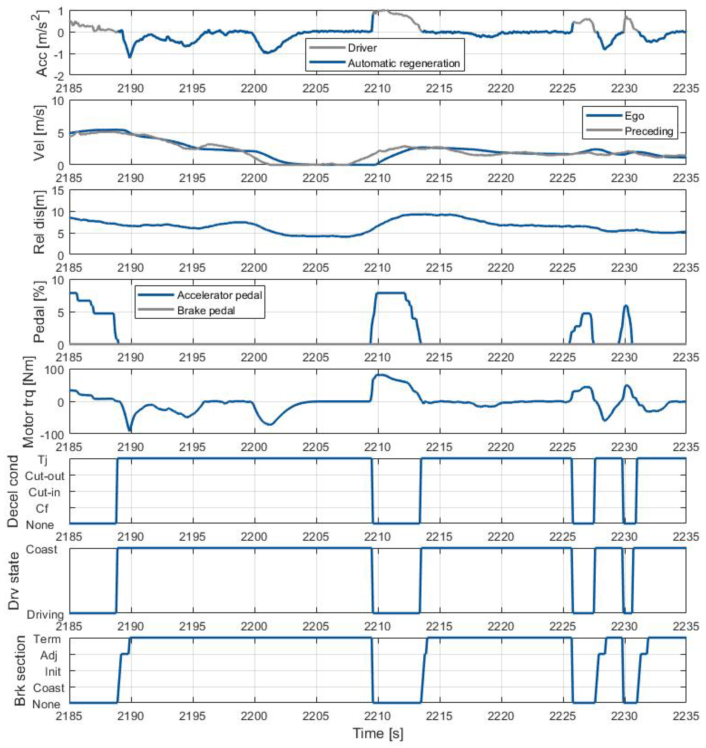
Figure 17 shows the results of automatic regeneration in traffic jam situations. The velocity in this profile is under 6 m/s, and the relative distance is under 10 m. Therefore, the deceleration condition is determined as “traffic jam.” When the relative distance is under 10 m, keeping a safe distance from the leading car is most important, so the braking section enters into the adjustment section directly. Then, the deceleration model generates deceleration, which is very similar to the reference acceleration. As shown in the fourth subplot, the driver does not push the brake pedal at all, but the vehicle speed and relative distance are controlled appropriately.

During the vehicle test, there were 251 deceleration situations. Among them, the driver pushed the brake pedal to decelerate in 30 situations, and deceleration was by automatic regeneration in 231 situations. That is, automatic regeneration reduced the amount of braking by 92% in the test driving route.

6.5. Learning Results

To check the tendency of the updated learning vector depending on the driver, three test drivers drove the test vehicle on the route shown in Figure 18. All drivers decelerated the vehicle not by using the SRS, but by pushing the brake pedal themselves. The driving situation was car-following with a leading car. The preceding vehicle decelerated while changing speed variously from 70 km/h to complete stop. To keep a safe distance, the three test drivers decelerated the vehicle based on their own driver characteristics. The learning vectors were updated online whenever the drivers finished decelerating.

Figure 19 shows the learning results of the learning vector for the initial jerk. The values of the reference parameter, which is from the driver’s driving, are also shown in the graph. As shown in the first subplot, driver 3 shows a tendency to have a bigger absolute value of the initial jerk compared to the other drivers overall. This means that driver 3 is a more aggressive driver who pushes the brake pedal more rapidly in the initial section.

Figure 20 and Figure 21 show the results of the online learning algorithm in the learning vectors for initial and adjustment distance. Commonly in both figures, the learning vectors of driver 3 are located lower than those of the other drivers, which means that driver 3 started the initial and adjustment section when the relative distance was reduced enough.

Figure 22 shows the learning results of the velocity difference. Although the velocity difference does not have a correlation with the initial index, its learning vector is based on the initial index to manage the learning vector with the same method as the other learning vectors. As shown in the first subplot of the figure, the learning vector of driver 2 has a bigger value than that of the other drivers, which means that driver 2 tends to decelerate to much slower than the preceding vehicle.

7. Conclusions

This study proposes automatic regeneration based on the parametric deceleration model reflecting driver characteristics online. Based on an analysis of the deceleration profile, we split it into four braking sections: coast, initial, adjustment, and termination. Then, the parametric deceleration model was designed considering the features of each braking section. In addition, it can reflect the driver’s characteristics because it consists of driver parameters calculated based on the learning vector. To update the driver characteristics online, the online learning algorithm was designed. It updates the learning vector, which manages the driver characteristics by comparing the planning results and driving data.

The automatic regenerative braking based on the proposed algorithm was validated through vehicle tests on urban and highway roads. The planning results show a similar shape to human driving, such as coasting behavior, and the results of automatic regeneration show that a safe distance is maintained in car-following and traffic jam situations. Moreover, the learning results show that the learning vectors are updated differently according to the driver’s deceleration pattern.

By the suggested automatic regeneration, the amount of braking decreased by 92% on the test driving route. Most of the range that the suggested algorithm did not cover was decelerating for a static object such as a speed hump, cornering at intersections, and following speed limits. This information can be acquired through the navigation device of the test vehicle. Therefore, automatic regeneration will be extended using the information from navigation devices in the future.

References

1. Lee, J.; Kim, H. Control Apparatus and Method for Regenerative Braking of Eco-Friendly Vehicle. KR Patent 101558772, 7 Octember 2015. [Google Scholar]
2. Lin, C.L.; Hung, H.C.; Li, J.C. Active control of regenerative brake for electric vehicles. Actuators 2018, 7, 84. [Google Scholar] [CrossRef]
3. Xu, G.; Li, W.; Xu, K.; Song, Z. An intelligent regenerative braking strategy for electric vehicles. Energies 2011, 4, 1461–1477. [Google Scholar] [CrossRef]
4. Gong, X.; Qian, L.; Ge, W.; Wang, L.F. Research on the Anti-Disturbance Control Method of Brake-by-Wire Unit for Electric Vehicles. World Electr. Veh. J. 2019, 10, 44. [Google Scholar] [CrossRef]
5. He, R.; Tian, X.; Ni, Y.; Xu, Y. Mode transition coordination control for parallel hybrid electric vehicle based on switched system. Adv. Mech. Eng. 2017, 9, 1–12. [Google Scholar] [CrossRef]
6. Lv, C.; Zhang, J.; Li, Y.; Yuan, Y. Mode-switching-based active control of a powertrain system with non-linear backlash and flexibility for an electric vehicle during regenerative deceleration. Proc. Inst. Mech. Eng. Part. D J. Automob. Eng. 2015, 229, 1429–1442. [Google Scholar] [CrossRef]
7. Liu, H.; Wei, H.; Zuo, T.; Li, Z.; Yang, Y.J. Fine-tuning ADAS algorithm parameters for optimizing traffic safety and mobility in connected vehicle environment. Transp. Res. Part. C Emerg. Technol. 2017, 76, 132–149. [Google Scholar] [CrossRef] [PubMed]
8. Gu, Y.; Hashimoto, Y.; Hsu, L.T.; Iryo-Asano, M.; Kamijo, S. Human-like motion planning model for driving in signalized intersections. IATSS Res. 2017, 41, 129–139. [Google Scholar] [CrossRef] [Green Version]
9. Gu, T.; Dolan, J.M. Toward human-like motion planning in urban environments. IEEE Intell. Veh. Symp. Proc. 2014, 350–355. [Google Scholar] [Green Version]
10. Hasenjager, M.; Wersing, H. Personalization in advanced driver assistance systems and autonomous vehicles: A review. In Proceedings of the 2017 IEEE 20th International Conference on Intelligent Transportation Systems (ITSC), Yokohama, Japan, 16–19 Octember 2017. [Google Scholar]
11. Bifulco, G.N.; Simonelli, F.; Di Pace, R. Experiments toward an human-like Adaptive Cruise Control. IEEE Intell. Veh. Symp. Proc. 2008, 919–924. [Google Scholar]
12. Bifulco, G.N.; Pariota, L.; Simonelli, F.; Pace, R. Di Development and testing of a fully adaptive cruise control system. Transp. Res. Part. C Emerg. Technol. 2013, 29, 156–170. [Google Scholar] [CrossRef]
13. Lefèvre, S.; Carvalho, A.; Gao, Y.; Tseng, H.E.; Borrelli, F. Driver models for personalised driving assistance. Veh. Syst. Dyn. 2015, 53, 1705–1720. [Google Scholar] [CrossRef]
14. Treiber, M.; Hennecke, A.; Helbing, D. Congested traffic states in empirical observations and microsopic simulations. Phys. Rev. E 2000, 62, 1805–1824. [Google Scholar] [CrossRef] [PubMed]
15. Khodayari, A.; Ghaffari, A.; Kazemi, R.; Braunstingl, R. A Modified Car-Following Model Based on a Neural Network Model of the Human Driver Effects. IEEE Trans. Syst. Man Cybern. Part. A Syst. Hum. 2012, 42, 1440–1449. [Google Scholar] [CrossRef]
16. Chong, L.; Abbas, M.M.; Medina Flintsch, A.; Higgs, B. A rule-based neural network approach to model driver naturalistic behavior in traffic. Transp. Res. Part. C Emerg. Technol. 2013, 32, 207–223. [Google Scholar] [CrossRef]
17. Mehar, A.; Chandra, S.; Velmurugan, S. Speed and acceleration characteristics of different types of vehicles on multi-lane highways. Eur. Transp. Trasp. Eur. 2013, 1–12. [Google Scholar]
18. Yang, G.; Xu, H.; Wang, Z.; Tian, Z. Truck acceleration behavior study and acceleration lane length recommendations for metered on-ramps. Int. J. Transp. Sci. Technol. 2016, 5, 93–102. [Google Scholar] [CrossRef] [Green Version]
19. Yang, G.; Xu, H.; Tian, Z.; Wang, Z. Vehicle Speed and Acceleration Profile Study for Metered On-Ramps in California. J. Transp. Eng. 2015, 142, 04015046. [Google Scholar] [CrossRef]
20. Bham, G.H.; Benerkohal, R.F. Acceleration Behavior of Drivers in a Platoon. In Proceedings of the First International Driving Symposium on Human Factors in Driver Assesment, Training and Vehicle Design, Aspen, CO, USA, 14–17 August 2001. [Google Scholar]
21. Zhang, Y.; Lv, J.; Wang, W. Evaluation of vehicle acceleration models for emission estimation at an intersection. Transp. Res. Part. D Transp. Environ. 2013, 18, 46–50. [Google Scholar] [CrossRef]
22. Milanes, V.; Shladover, S.E.; Spring, J.; Nowakowski, C.; Kawazoe, H.; Nakamura, M. Cooperative adaptive cruise control in real traffic situations. IEEE Trans. Intell. Transp. Syst. 2014, 15, 296–305. [Google Scholar] [CrossRef]
23. Milanés, V.; Shladover, S.E. Modeling cooperative and autonomous adaptive cruise control dynamic responses using experimental data. Transp. Res. Part. C Emerg. Technol. 2014, 48, 285–300. [Google Scholar] [CrossRef] [Green Version]
24. McClamroch, N.H. Space vehicle dynamics and control. Automatica 2001, 37, 2077–2078. [Google Scholar] [CrossRef]
25. Rajamani, R.; Zhu, C. Semi-autonomous adaptive cruise control systems. IEEE Trans. Veh. Technol. 2002, 51, 1186–1192. [Google Scholar] [CrossRef]
26. Ploeg, J.; Serrarens, A.F.A.; Heijenk, G.J. Connect Drive: Design and evaluation of cooperative adaptive cruise control for congestion reduction. J. Mod. Transp. 2011, 19, 207–213. [Google Scholar] [CrossRef]
Figure 1. Overall structure of the algorithm.
Wevj 10 00058 g001
Figure 2. Flowchart of driving states.
Wevj 10 00058 g002
Figure 3. Deceleration profile in general car-following.
Wevj 10 00058 g003
Figure 4. Profiles of v d i f f _ r e f and v r e f , t e r m .
Wevj 10 00058 g004
Figure 5. Correlation of coast distance and initial distance.
Wevj 10 00058 g005
Figure 6. Correlation of initial distance and adjustment distance.
Wevj 10 00058 g006
Figure 7. Comparison of measured deceleration and constant acceleration model.
Wevj 10 00058 g007
Figure 8. Correlation analysis of the initial jerk.
Wevj 10 00058 g008
Figure 9. Learning vector of initial jerk.
Wevj 10 00058 g009
Figure 10. Gaussian distribution using value of initial index.
Wevj 10 00058 g010
Figure 11. Convergence of learning vector when learning rate is 0.2.
Wevj 10 00058 g011
Figure 12. Learning vector of initial jerk before update.
Wevj 10 00058 g012
Figure 13. Acceleration controller.
Wevj 10 00058 g013
Figure 14. Route for vehicle test.
Wevj 10 00058 g014
Figure 15. Vehicle test results on urban roads.
Wevj 10 00058 g015
Figure 16. Test results in general car-following situations.
Wevj 10 00058 g016
Figure 17. Test results in traffic jam situations.
Wevj 10 00058 g017
Figure 18. Test route for validation of online learning algorithm.
Wevj 10 00058 g018
Figure 19. Learning results of learning vector for initial jerk.
Wevj 10 00058 g019
Figure 20. Learning results of learning vector for initial distance.
Wevj 10 00058 g020
Figure 21. Learning results of learning vector for adjustment distance.
Wevj 10 00058 g021
Figure 22. Learning results of learning vector for velocity difference.
Wevj 10 00058 g022