1. Introduction
In these days, the intelligent transfer system forcefully affects many advanced driver assistance systems (ADAS) that enhance the driver convenience and energy efficiency. A smart regenerative braking (SRB) system of electric vehicles is one ADAS application which uses forecasting information on braking situations [
1,
2,
3]. This SRB system automatically controls the regenerative torque of the electric motor when the vehicle should be braking. The vehicle can decelerate without the driver’s physical brake pedaling. Thus, it leads to driver convenience as it excludes the driver’s action, and the avoidance of frequent braking that harnesses the energy that dissipates through a brake disk.
To attain both convenience and energy efficiency, the regenerative torque control system requires an appropriate deceleration planning algorithm to use for the control set-point of the regenerative torque [
4,
5]. This planning algorithm can recognize the diverse deceleration conditions such as the stop condition in front of the traffic light, decelerating before the curvature load, speed limit or the condition when the preceding vehicle is decelerating. Then, it should determine the deceleration profile that can guarantee safety by the automatic braking. Furthermore, the driver can feel the heterogeneity because the automatic braking control is difficult to apply to the driving style of the individual drivers [
2,
6,
7].
The SRB system requires a deceleration specified planning algorithm to determine the set-point for regenerative torque control. In general, the continuous optimization method based planning is widely applied to determine the vehicle trajectory for autonomous longitudinal vehicle control applications, such as an adaptive cruise control system [
8,
9,
10]. The optimization method-based planning algorithm determines the optimal vehicle trajectory to minimize the selected cost function and constraints. This numerical optimization method using the mathematical model offers the advantages that the determined trajectory can apply to diverse driving conditions. However, this method cannot consider individual driver characteristics efficiently.
The other method is an intelligent driver model (IDM) based planning. This method was introduced at [
11] and provides the deceleration profile by reflecting the individual driver characteristics. The model consists of the mathematical equation and model parameters. The model configures the model parameters according to the driver characteristics. In our previous research, the deceleration specified planning algorithm was proposed based on the intelligent driver model for the SRB system [
12]. This can determine the appropriate deceleration profile at specific deceleration conditions. However, the model should cover the diverse and complex driving conditions to apply to real driving situations.
This paper proposed a multi-level deceleration planning algorithm to get the advantages of the two introduced planning methods. The planning management, which is a high-level algorithm determines the weight factor that is a merging rate among the two planning algorithms. This planning management is designed based on the reinforcement learning algorithm. Since the reinforcement learning algorithm can secure the optimal solution as a result of repeated action, it has been widely applied to complex systems [
13,
14,
15,
16]. Thus, the planning management can select the optimal planning results for nonlinear complex driving situations with uncertainties. By learning, the planning management gives an appropriate vehicle trajectory for the SRB system for various deceleration conditions while reflecting individual driver characteristics. Thus, the main contribution of this paper is the application of a driver model as a planning algorithm to reflect the driving style, and the design of the reinforcement learning algorithm to find optimal planning results for driver intention, safety, and energy efficiency.
This paper is organized as follows: In
Section 2, the algorithm overview is introduced. The proposed algorithm consists of simulation models and deceleration planning algorithms.
Section 3 describes the simulation models that are the vehicle model and battery model. The model-based planning and optimization-based planning algorithms are explained in
Section 4. Then, the planning management algorithm based on reinforcement learning is described in
Section 5.
Section 6 shows the validation results of the proposed algorithm.
2. Algorithm Overview
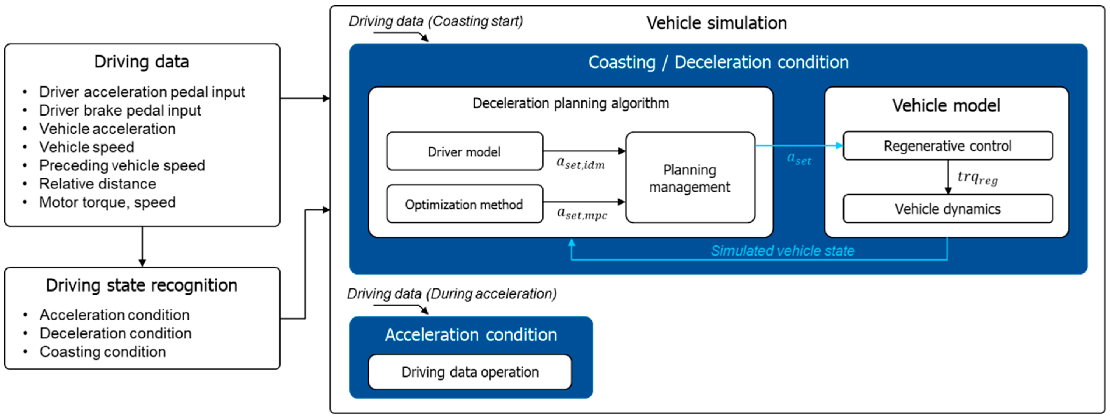
The SRB system decelerates the electric vehicle without the drivers braking pedal actions. Thus, the proposed deceleration planning algorithm is applied when the vehicle faces deceleration situations. The vehicle driving data was used to simulate the deceleration situations. As shown in
Figure 1, the driving data consists of the drivers pedal input, current vehicle acceleration, velocity, preceding vehicle speed, relative distance to the preceding vehicle, electric motor information, and battery information. Using this driving data, the driving state recognition algorithm determines the current vehicle driving state. The vehicle driving state is classified as an acceleration condition, deceleration condition, and coasting condition. When the driver pushes the acceleration pedal, the driving state is determined as the acceleration condition. On the other hand, the driving state is determined as the deceleration condition when the driver pushes the brake pedal, and the driving state is changed to the coasting condition when the driver releases the foot from the acceleration pedal.
When the driving state changes to the coasting condition, it means the driver decelerates due to some deceleration causes. At this time, the vehicle simulation starts using the driving data that the coasting starts. When the vehicle simulation starts, the deceleration planning algorithm determines the optimal vehicle acceleration set-point to the current vehicle of the coasting start driving data. The SRB algorithm generates the regenerative torque to trace the vehicle acceleration set-point from the deceleration planning algorithm. Then, the vehicle and battery models simulate the vehicle states using their dynamics models. The simulated vehicle states are used for the deceleration planning algorithm to determine the vehicle acceleration set-point at the next simulation step. Consequently, during the coasting and deceleration conditions, the deceleration planning algorithm determines the optimal vehicle acceleration set-point based on the proposed algorithm with the simulated vehicle states iteratively. Thus, based on the simulation results, the autonomous deceleration results by the SRB system can be verified.
The vehicle simulation does not work during the acceleration condition because the driver controls the vehicle acceleration by pedaling the acceleration pedal. In this case, the vehicle simulation results are bypassed using the driving data.
3. Simulation Environments
The algorithm was designed in a python environment because the python environment easily approaches to many deep learning libraries. In the python environment, the electric vehicle model with a battery model and the planning algorithms were designed to simulate and determine the planning management.
3.1. Vehicle Model Description
A vehicle simulation model contains the power source model and drive train model, as shown in
Figure 2. These two models simulate only the longitudinal vehicle behavior because the proposed SRB system assists the longitudinal vehicle deceleration. The power source model that represents the state of electric devices simulates the consumed electric power to generate the motor torque. According to the generated motor torque from the power source model, the drive train model simulates the longitudinal vehicle dynamics. The inputs to the vehicle model are determined from the driver interpretation and regenerative control module. Those modules determine the generated motor torque of the electric motor model.
The well-known Chen’s two-stage model was used to design the battery model [
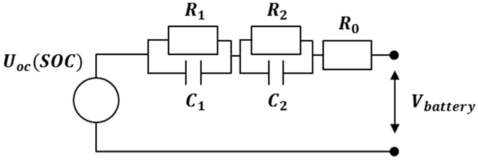
17]. Based on Chen’s two-stage model, the battery model estimates the battery states according to the state of the charge (SOC) as Equation (1). This model can represent the battery characteristics of the transient conditions. Since the model contains two RC circuit as shown in
Figure 3, the model can represent not only long-term transient behavior, but also short-term transient behavior well. As a result, the battery model can calculate the SOC decrement depending on the consumed electric power by the motor and can determine the battery status according to the calculated SOC.
The first order dynamic model based on Newton’s second law was determined to describe the longitudinal vehicle dynamics as Equations (2)–(4). According to the model, vehicle acceleration is calculated using the fraction force from the power source and drag force from the drag system, which describes the air and rolling resistance as Equation (4). The power source generates the motor torque using the battery power. Then, the drive train transfers the motor torque with the deceleration gear ratio. The traction force to the tire wheel is determined using this torque.
3.2. Parameter Identification
The designed vehicle model can be configured as accustoming the model parameters such as the battery register, driver train inertia, vehicle air coefficient, or vehicle mass. The model parameters were determined through the parameter identification process using the real vehicle driving data to simulate the vehicle operation as similarly with the real experiment vehicle. KONA electric vehicle of Hyundai Motor Company was used to acquire the driving data. The vehicle experiments were conducted in various driving cases. The driving cases contain the car-following situation on the straight load, urban driving, highway driving, and the uphill driving. The battery parameters were also identified using the driving data on various battery SOC ranges.
Based on the nonlinear least-square solver with the trust-region-reflective algorithm [
18,
19], the parameters of vehicle and battery models were identified.
Figure 4 shows the modeling results of the vehicle and battery when the vehicle repeats the acceleration and deceleration. According to the torque control inputs, the vehicle model well simulates the longitudinal vehicle behavior as shown in the figure. However, the rotational dynamics of a vehicle shaft from the motor to the wheel was also simulated for similarity with real driving data. The modeling results of the battery model is validated by comparing the battery current.
Table 1 and
Table 2 describe the parameter values.
3.3. Regenerative Torque Control
As mentioned above, the regenerative control module can conduct the regenerative control of the electric vehicle. If the motor generates the negative torque, the crankshaft and vehicle decelerate when the vehicle is driving. At this time, this negative torque charges the battery energy by the regeneration.
Figure 5 shows the result of regenerative control using the simulation models. The vehicle repeats the acceleration and deceleration as shown in a vehicle speed graph. The orange dot line of the motor torque and battery SOC are the results with the regenerative control and the solid blue line shows the deceleration results by pushing the brake pedal. As shown in
Figure 5, the regenerative torque which is the minus motor torque, can decelerate the vehicle and can charge the battery SOC when the regeneration occurs.
4. Planning Algorithms
The SRB system controls the regenerative torque automatically according to the deceleration driving environment without the driver intervention. Thus, the important things of the planning algorithm for the SRB system are that the planning algorithm generates the deceleration set-point which guarantees the safety for the deceleration conditions. Furthermore, it can reflect the driver driving style to minimize the heterogeneity by the automatic braking. To secure these requirements, two planning algorithms were proposed: The IDM based planning and the optimization method-based planning.
4.1. Intelligent Driver Model-Based Planning
The IDM based planning was designed based on the parametric deceleration model, which was introduced in our previous research [
12]. This model is designed based on the well-known IDM [
11]. The model consists of some parametric equations and model parameters. It can estimate the deceleration profile using the mathematical equations about the physical meaning and some model parameters. Since the model parameters can represent the individual driver characteristics, the planning algorithm which uses this parametric model can also reflect the individual driving style.
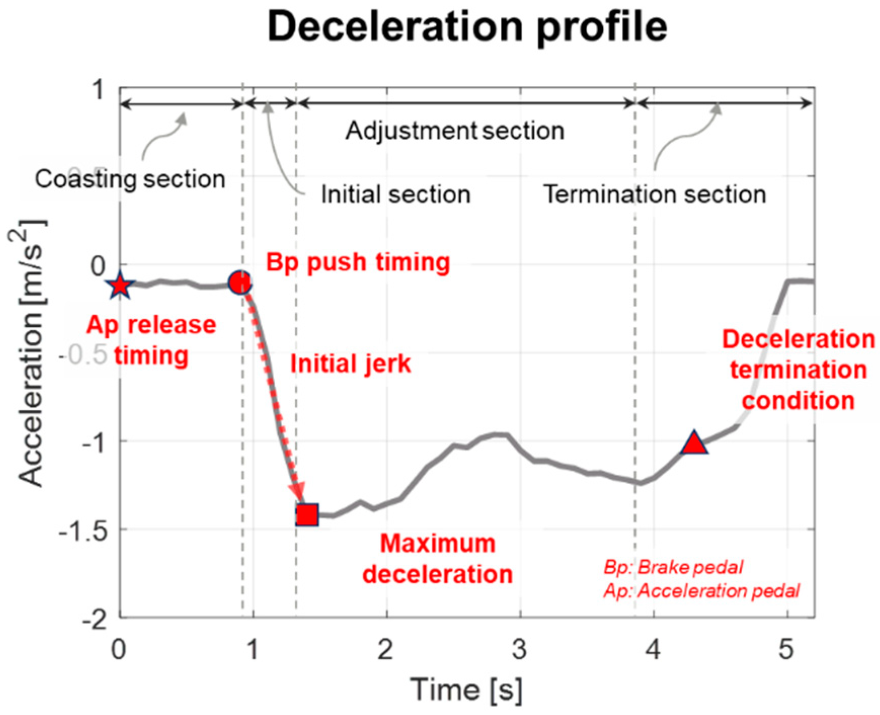
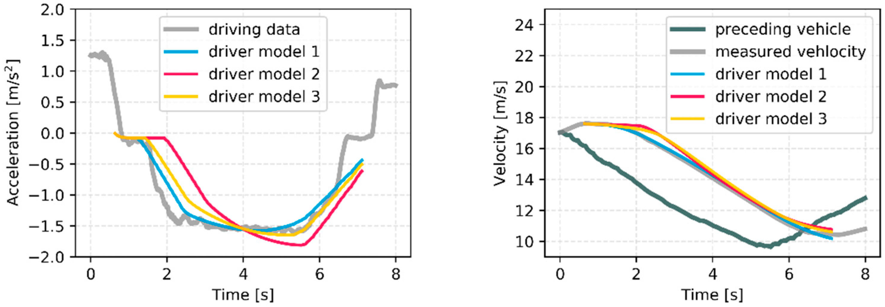
Figure 6 describes the model parameters. When the driver decelerates, the braking timing, initial jerk, and specific acceleration values especially represent the driver characteristics. Thus, these physical values were determined as the model parameters. Furthermore, when the deceleration is terminated, the termination relative velocity to the preceding vehicle also represents the driver characteristics.
Furthermore, the braking section wa defined as the period according to the driver’s deceleration behavior and model parameters. Each braking section means as follows. The coasting section means the driver’s pedal shifting time from the acceleration pedal to the brake pedal. When in the initial section, the driver pushes the brake pedal until the vehicle deceleration reaches a specific value. The acceleration slope on the initial section is determined as the initial jerk parameter. After the initial section, the driver adjusts the brake pedal to converge to the velocity condition for the preceding vehicle. Then, the driver controls the brake pedal to keep a safe distance. Using these braking sections, the model can represent the deceleration characteristics in detail.
4.1.1. Description of the Prediction Process
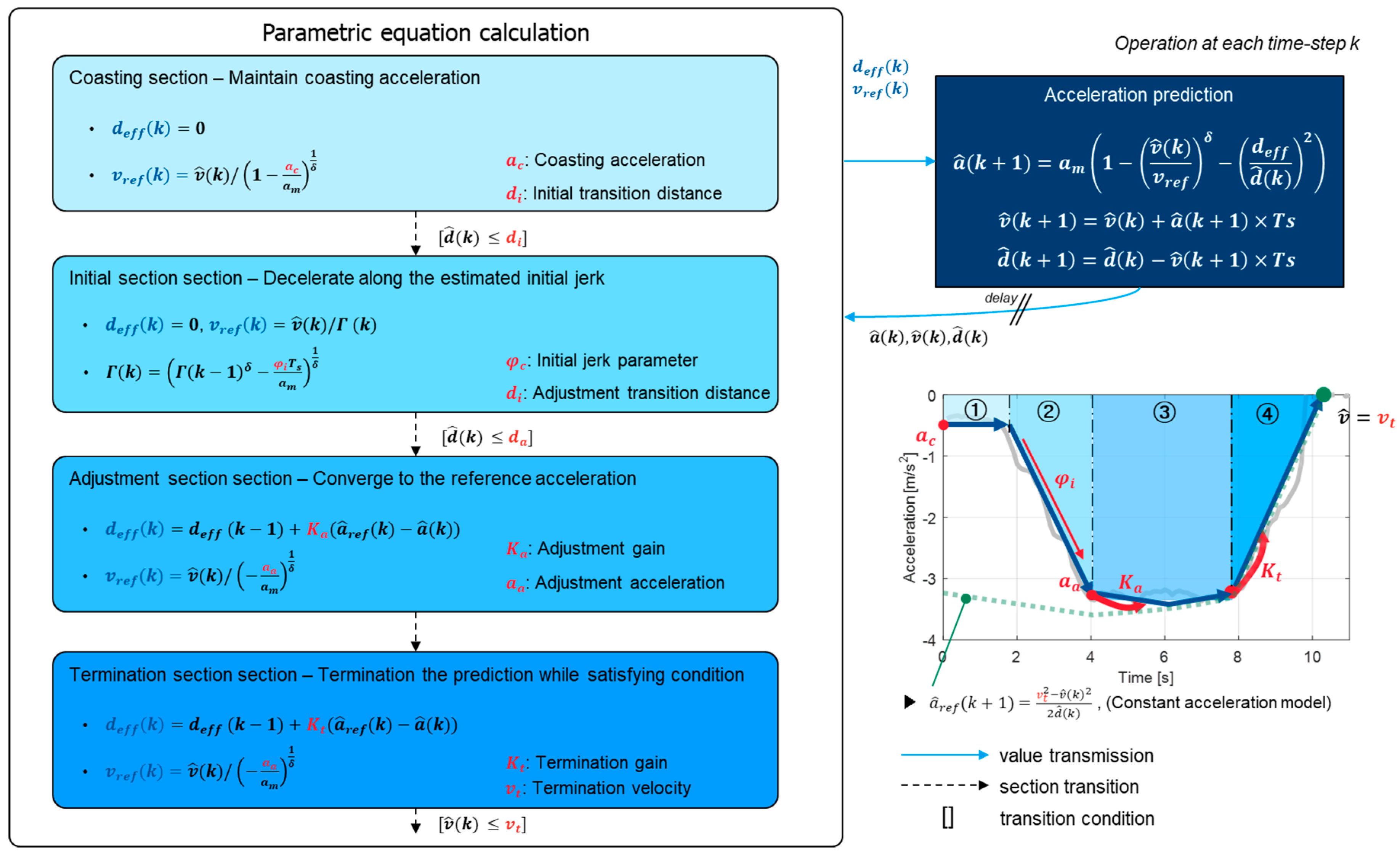
Equation (5) describes the parametric deceleration model. The reference velocity
and effective distance
are designed as the parametric equations and the parametric equations are determined according to the braking section and model parameters as shown in
Figure 7.
Figure 7 shows the detailed equation about the parametric equations according to the braking section using the model parameters. As shown in the estimated deceleration profile, the parametric equation model reflects the deceleration characteristics of each braking section as those described above.
At the coasting section, the reference velocity equation is determined to maintain the coasting acceleration
. When the predicted vehicle state satisfies the transition condition, the algorithm transmits the braking section. The transition condition of the coasting section is that the predicted relative distance is closer than the initial transition distance parameter
. The braking section is changed to the initial section, and then the model determines the reference velocity using the velocity ratio
to imitate the initial acceleration slope. This initial acceleration slope is determined as the initial jerk parameter
. After the adjustment section starts, the effective distance is determined to converge the predicted acceleration to the reference acceleration
. The reference acceleration is an acceleration profile from the constant acceleration model to satisfy the termination condition of deceleration as shown in
Figure 7. Finally, the model traces the reference acceleration until the deceleration terminates at the termination section. The difference between the adjustment section and the termination section is the gain parameters which determine the effective distance.
4.1.2. Parameter Learning Algorithm
As mentioned in the introduction, the model parameter should be updated according to the driving data of each driver on real-time driving conditions. The learning algorithm, which can be applied to the real-time embedded system, was designed. To manage the model parameter for the embedded suitable update algorithm, the vector value and its index for each model parameter were determined. The vector value means the parameter value of the model parameter, and the vector index means the driving condition which affects to the model parameter. Thus, the learning algorithm selects the parameter value among the vector values according to the driving conditions by using the vector index.
The braking data of three drivers were acquired by the vehicle driving experiment to update the parameter vectors. The initial values of the parameter vector were defined using the acquired data. The reference parameter values were calculated using the driving data of the individual driver every time a deceleration occurred. Then, using the reference parameter, the vector array of each parameter was updated. Consequently, the model parameters were updated for each deceleration driving according to the individual driver characteristics of the three drivers.
Figure 8 shows the parameter values and its index values for each parameter. As shown in the figure, the parameter initial jerk correlates to the coast index parameter which means the initial vehicle states. It describes, when deceleration starts, the driver pushing the brake pedal more aggressively as the relative distance is small. The relative distance parameters correlate to the relative distance at the previous braking section. The initial transition distance correlates to the relative distance when the coasting section starts, and the adjustment transition distance is correlated to the relative distance when the initial section starts. Those mean that the driver tends to keep the same time to collision in an early braking situation.
Figure 8 also shows the base vector which is an initial value of the parameter vector and the learning results of three drivers. The result describes the driving characteristics. Then, each updated parameter vector is used to learn the planning management.
4.1.3. Planning Results According to Each Driver
Figure 9 shows the planning results through the proposed model-based planning algorithm. The planning algorithm is applied to the same deceleration start conditions: The ego vehicle velocity, preceding vehicle velocity, and acceleration start condition. However, the algorithm uses different learned parameter vectors for the three drivers. As shown in the figure, the model generates different deceleration profiles according to the individual driver. Depending on the learning results, the driver characteristics for driver 2 shows that the transition distance is closer than other drivers, and that characteristic is represented on the planning result for driver 2. The driver 1 and driver 3 have the same transition distance. However, the initial jerk characteristic of driver 1 is more aggressive than driver 3. Thus, the planning result about driver 1 represents more rapid deceleration at an early braking stage. Of course, the proposed three driver’s driving style cannot represent all driving characteristics. However, this algorithm can represent another driving style other than the three drivers by updating the model parameter using the real driving data of other driving characteristics.
4.2. Optimization Method Based Planning
The other planning method is an optimization-based planning algorithm. This planning algorithm determines the optimal deceleration trajectory using the mathematical model with a cost function and constraints. Generally, the longitudinal vehicle dynamics model is applied to the mathematical model, and the vehicle velocity and relative distance are used as the state values of the mathematical model because this deceleration planning algorithm should consider these coupled driving conditions. The cost function is defined to minimize the error of defined states. Furthermore, this cost function adjusts to the driving conditions as well as the constraints. It can lead the optimal deceleration trajectory on the various deceleration conditions by solving the cost function with constraints.
4.2.1. Model Predictive Control Scheme
The linear model predictive control (MPC) algorithm is used to solve this optimization problem. The MPC algorithm predicts the future state using the mathematical system model and finds optimal inputs by minimizing the predictive cost. Generally, the MPC scheme is determined as Equations (6) and (7) those contain the cost function, system model, and constraints.
Minimize
, subject to
The cost function
consists of the weighted sum of the tracing error
and control effort
during the prediction horizon
. Each term has weight values
. The model predictive controller obtains the optimal input
to minimize this cost value with constraints.
is a state that consists of the relative distance
and relative velocity
and input is the vehicle acceleration. The tracing error
is defined as the difference between the current state and the desired state value
. In this model, the desired state value is determined in
Table 3. The desired state contains the desired relative distance parameter and desired relative velocity, respectively. The desired relative distance is determined to maintain a safe distance from the preceding vehicle, and the desired relative velocity is determined as the zero value to keep the preceding vehicle speed. The weight values
and
give weighting to each error state for optimization. There are two constraints, the equality constraint and inequality constraint. The equality constraint represents the system equation of the longitudinal vehicle dynamics. The future state of the relative distance and velocity are calculated according to the first-order discrete dynamics according to the input acceleration. Based on this system matrix and current state, the future state is calculated. The obtained input value is also constrained in the acceleration range from 0 m/s
2 to −5 m/s
2.
4.2.2. Planning Results Using the MPC Algorithm
The weight values for each state and the prediction horizon affect the planning results of the MPC algorithm. To apply the MPC algorithm to the deceleration planning, the weight values and prediction horizon at the same deceleration case of model-based planning algorithm were configured. At first, the prediction horizon varied when the weight values were fixed.
Figure 10 shows the effects of the prediction horizon variation. When the prediction horizon is ten steps, the state error of the relative distance cannot converge to the zero value. It means that the smaller prediction horizon does not guarantee to maintain the safe distance. On the other hand, the planning result is aggressive when the prediction horizon is 20 steps. It might cause an uncomfortable feeling to the driver. In the same manner, the state value does not converge to their desired state value, when each weight value is too much small, and the control results are aggressive when each weight value is too much large as shown in
Figure 11 and
Figure 12. Thus, the prediction horizon value and each weight value were configured as follows. The value of prediction horizon
N is 15, weight value
qdf is 4, and weight value
qvf is 0.1.
5. Planning Management
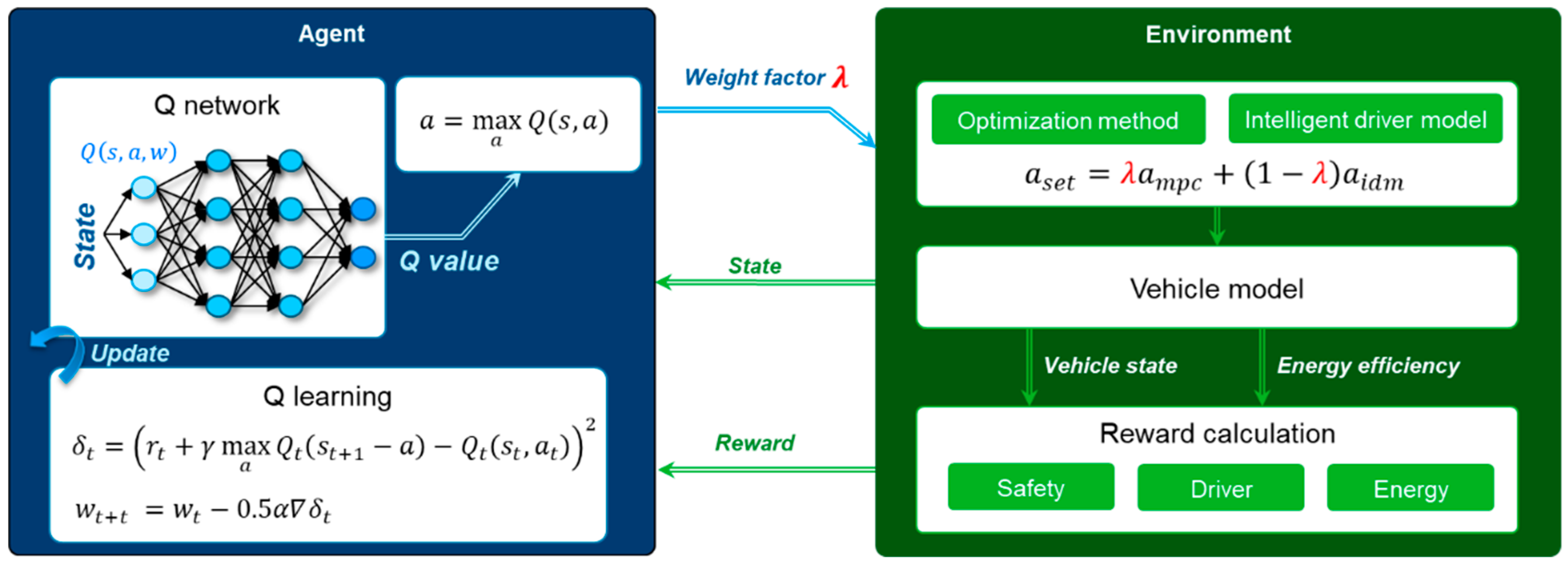
As mentioned in the introduction section, the proposed two planning algorithms have their advantages for applying to the SRB system, respectively. The driver model-based planning algorithm can reflect the driver characteristics to reduce the heterogeneity by automatic braking control. On the other hand, the optimization-based planning algorithm can determine an appropriate deceleration trajectory on the various deceleration conditions while ensuring safety. To take these advantages for the SRB system, the planning management algorithm determines the optimal planning result. The planning management selects the optimal weight factor, and this weight factor determines the planning ratio among the model-based planning and optimization-based planning as Equation (8)
where
is a determined deceleration set-point,
is a planning result from the optimization method which is the MPC algorithm, and
is a planning result from the IDM. The value range of the weight factor
is from 0 to 1. If the manager selects the weight factor as 1, the deceleration set-point is determined as the planning result from the optimization method. If the management selects the weight factor as 0, the planning result from the intelligent model is dominant.
5.1. Overview of the Reinforcement Learning Algorithm
It is difficult for planning management to determine the optimal weight value because the drivers can face diverse deceleration conditions. Thus, the planning management learned to select the optimal weight value based on the reinforcement learning algorithm because this algorithm can handle the nonlinear and complex problems as learning by itself [
20,
21,
22]. A basic concept of the reinforcement learning algorithm is that an agent selects an optimal action in an environment to maximize the cumulative future reward. The reinforcement algorithm is normally designed based on the Markov decision process (MDP) by the interaction of the agent and environment. MDP deals with bellow features
.
is a state that represents the current environment.
is an action of the agent.
is a reward from the environment. The agent selects the action to make the environment give a maximum reward at the current state. Then, the state of the environment is changed according to the action and the transition probability model
to generate the reward for each state and action.
The reinforcement learning algorithm defines the value function of each current state to determine the future cumulative reward according to the current state. Thus, the cumulative future reward should be estimated, at first. To estimate the cumulative future reward from the current state, the value function
is defined as Equation (9). At this time, the discounted factor
is applied to focus on the current reward. The value function of the current states can be reformulated as a recursion expression by the Bellman theory [
22]. As a result, the optimal policy of the agent is a selection of an action to maximize the value function at the current state. The next step is determining the cumulative reward according to, not only the current state, but also to taking action. To consider the action and the cumulative reward, the action-value function
is defined as Equation (10). While the value function means the future cumulative reward at the current state
, the action-value function means the future cumulative reward by taking action
at the current state
. Thus, the agent can select the optimal action by maximizing this action-value function at the current state.
In order to estimate the future cumulative reward, it is crucial to update the action-value function exactly. A Q-learning algorithm is one reinforcement algorithm which updates the action-value function based on the simple value iteration update using the old
value and new information by taking action as Equation (11). The learning rate
determines the update rate of the learned value
. The learned value is determined using the current reward and the maximum
value of the next state that depends on both the previous state and the selected action. Through this learning algorithm, the action-value function is updated according to the reward at the current state that occurs by taking action.
5.2. Reinforcement Learning Algorithm for Planning Management
Figure 13 shows the proposed algorithm structure for optimal planning of the SRB system based on reinforcement learning. The algorithm consists of the agent and environment. The agent selects the weight factor as an action. This weight factor determines the deceleration set-point among the planning algorithms. Then, the environment conducts the vehicle simulation according to the deceleration set-point. For the simulation results, the state and reward are also calculated on the environment. The state contains the vehicle velocity and acceleration, relative distance to the preceding vehicle, and battery state. Furthermore, the IDM state is defined as the state to reflect the individual driver characteristics to the agent.
The environment model calculates the reward. Since the agent selects the action to maximize the reward, the affordable definition of the reward function can determine the performance of the algorithm. To consider safety, comfort, and energy, the three reward functions and their scale values were determined as Equations (12)–(14). The safety reward function prevents the vehicle collision. This reward function generates the high penalty value when the relative distance between the vehicles is closer than the critical safety distance. In addition, the relative distance is smaller than the criterion value, and the reward function generates the normal penalty values to prepare for the collision. The comport reward function is related to the driver characteristics and driving data such as vehicle acceleration, velocity, and relative distance. The error value between the real-diving data and the control result is defined as the penalty value. To reduce this penalty, the agent selects the action for results which are similar to the driver’s driving data. The comfort reward function also uses the predicted value from the parametric model of each driver because the driving data that is used for learning can only reflect that measured driving situations. By using the parametric driver model, the agent can consider the driving characteristics of the individual driver even in other driving cases. The last reward function is an energy regeneration reward function. The increase of battery SOC by the regenerative control is determined as the positive reward of the algorithm. As determining the reward to secure the safety, driver intention, and energy efficiency, the proposed planning management algorithm can determine the optimal deceleration set-point for the SRB system.
The coefficient values , , of the driver intention reward are 1, 0.5, 0.5. The coefficient value of energy efficiency reward is 10. The value of critical distance for safety reward is 3 m, and coefficient values , are 10, 100.
5.3. Q Network Design and Learning Algorithm
The Q network is designed based on the deep neural network to estimate the optimal action value. At first, a sequential deep neural network was proposed. Since the sequential network is an advantage to the time-sequential data, it is suitable for the torque control application. In addition, since the deceleration characteristics of the driver are affected by the braking section which is time dominant period, the proposed q network is effective.
The recurrent neural network with a long short-term memory was used to the sequence neural network for Q value approximation. The recurrent neural network (RNN) is a representative sequence network because it takes the sequence input and predicts the sequential output. Using the hidden network, RNN extends the conventional feedforward neural network to handle the time-sequential information. However, the RNN model has a vanishing problem, and a blowing up gradient causes the long-term dependency problem. Long short-term memory (LSTM) architecture was introduced to solve this problem. The LSTM includes the memory cells in the hidden layer. This memory cell predicts the hidden state, like RNN. However, the cell state and gated structure can solve the limitation of RNN. The gate structure consists of the input gate, the output gate, and the forget gate. Equations (15)–(20) and
Figure 14 describe the LSTM algorithm.
The Q networks were determined based on the sequential neural network, and they were updated through the Q learning algorithm with the temporal difference learning method [
23]. The Q learning updates the network after taking action
of state
. In this time, the environment generates the immediate reward and state transition. Using these actions, states and rewards, the action-reward value is calculated. Then, using this action-reward value, the target value for Q network parameter update is determined as Equations (21) and (22).
6. Algorithm Validation Results
6.1. Learning Results for a Deceleration Case
The proposed planning management algorithm was learned in the simulation environment using the vehicle experiment data.
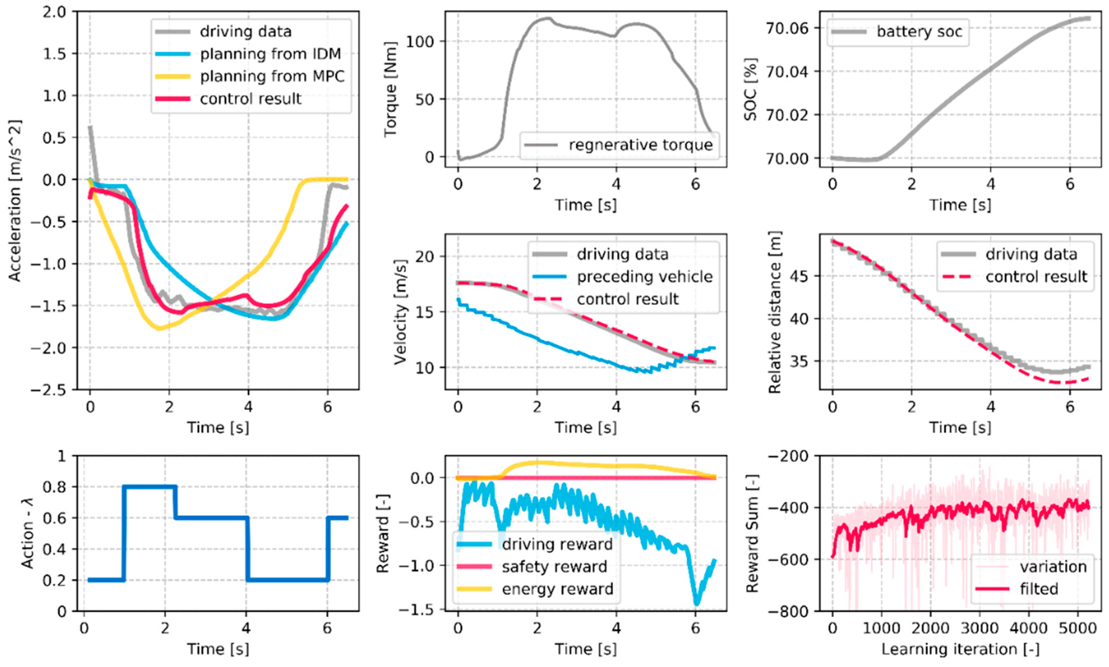
Figure 15 shows the learning results for one deceleration case. The left top figure shows the planning results and the control result for the vehicle acceleration. The MPC algorithm and IDM determine each deceleration profile. The planning management merges these two deceleration profiles according to the optimal weight factor
which the agent determines. The SRB system controls the vehicle to trace this deceleration set-point from the planning management. The control results show the SRB system decelerates the vehicle similar to the real driving data because the planning management selects the weight factor to reduce the negative driver reward. The energy reward increases according to the increase in the battery SOC by regenerative energy. Since the control result satisfies the safety criterion, there is no critical penalty reward. By the iterative Q-learning results, the summation of rewards increased as shown in the right bottom figure.
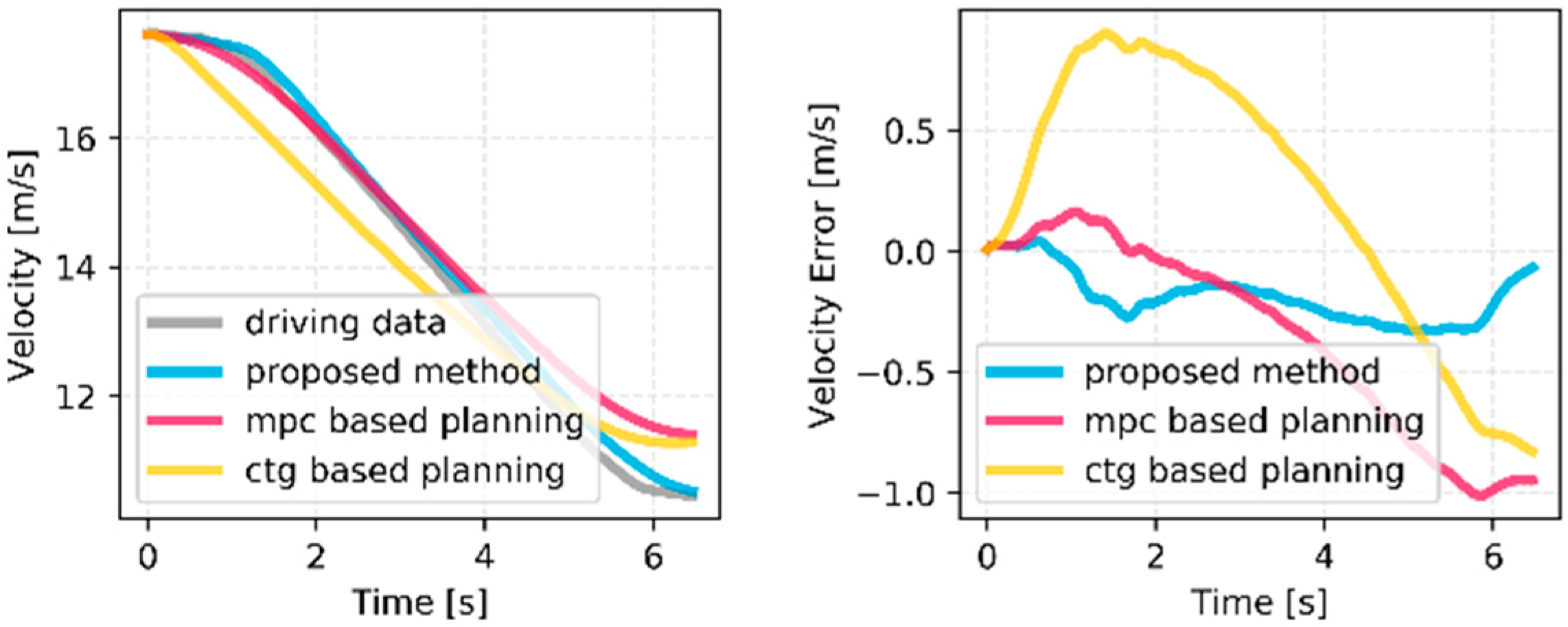
This study compared the planning results of the proposed algorithm to other planning results. As mentioned above, the MPC based longitudinal planning algorithm is a well-known optimization planning algorithm for car-following situations. In addition, the constant time gap (CTG) policy-based planning algorithm was also applied to compare the control results. This algorithm is commonly used in adaptive cruise control algorithms to ensure string stability [
24].
Figure 16 shows the control results of the vehicle velocity using the proposed algorithm, MPC based planning, and CTG based planning. Since the proposed planning algorithm can reflect the individual driving style by the learning algorithm, the control result based on the proposed algorithm is more related to the driver’s driving data than other planning algorithms. The detailed root-mean-square-error values are as follows. The proposed algorithm is 0.22 m/s, MPC based planning is 0.52 m/s, and CTG based planning is 0.60 m/s.
6.2. Validation Results for Various Driving Conditions
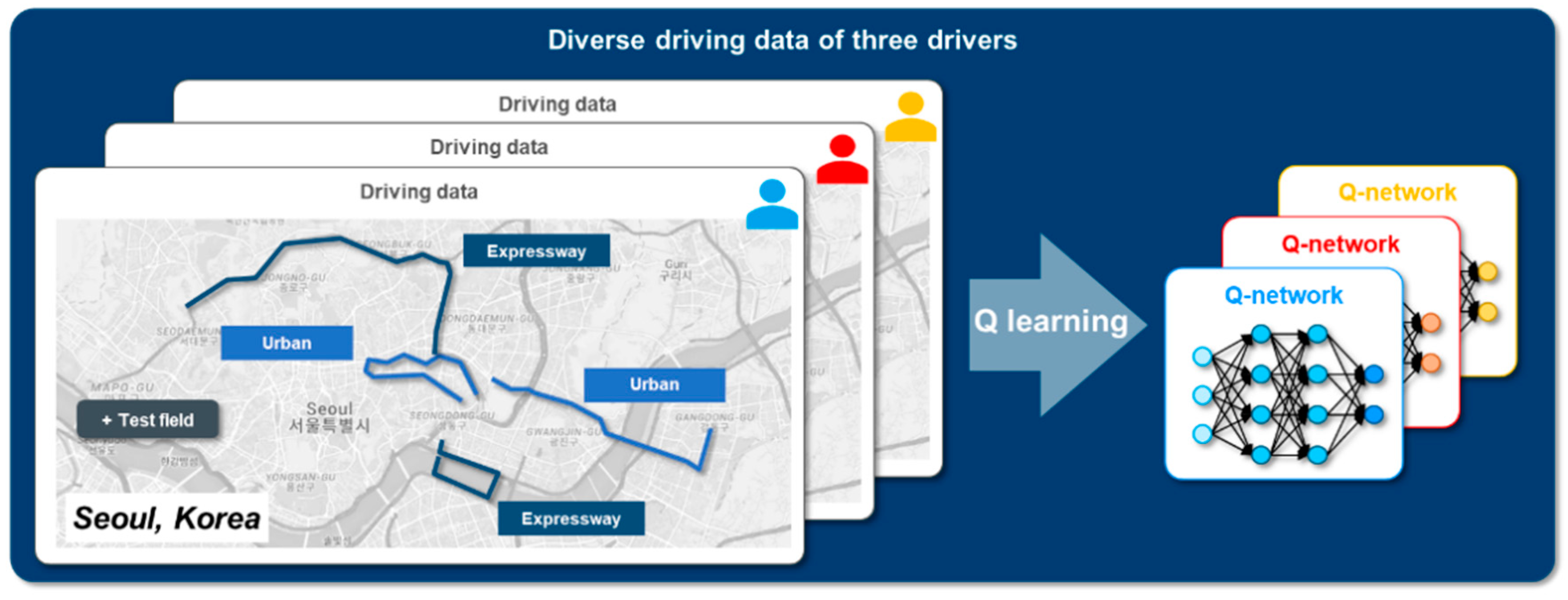
The proposed algorithm was validated using the vehicle experimental data. To represent the individual driver characteristics, three drivers conducted the vehicle experiment under various driving conditions as shown in
Figure 17. The experimental conditions were the urban driving condition, expressway driving conditions, and the proving ground. The learning algorithm updates Q network of the planning management according to the driver using the experimental data.
Figure 18 shows the control results for the various driving cases. There are three representative deceleration cases such as proving ground, expressway driving, and urban driving. Each column of the figure shows the planning and control results for each driving condition. On the proving ground, the vehicle repeats deceleration when the preceding vehicle is decelerating. Thus, the deceleration data is well organized and represents the test driver’s driving style explicitly. The control result of the proving ground also converged to the planning result from the IDM because the model was designed based on well-organized experiment data on the proving ground. The expressway result shows that planning management applies the appropriate planning result according to the deceleration conditions. If the deceleration condition is similar to the modeling condition of IDM, it means the model can represent the driver characteristics well, and the planning management selects the driver model-based planning. Contrary, the control results are reliant on MPC based planning if the deceleration condition is far from the modeling condition. In the urban driving condition, the SRB system controls the vehicle using the MPC based planning algorithm as the model cannot reflect the traffic jam situation as shown in the urban driving result.
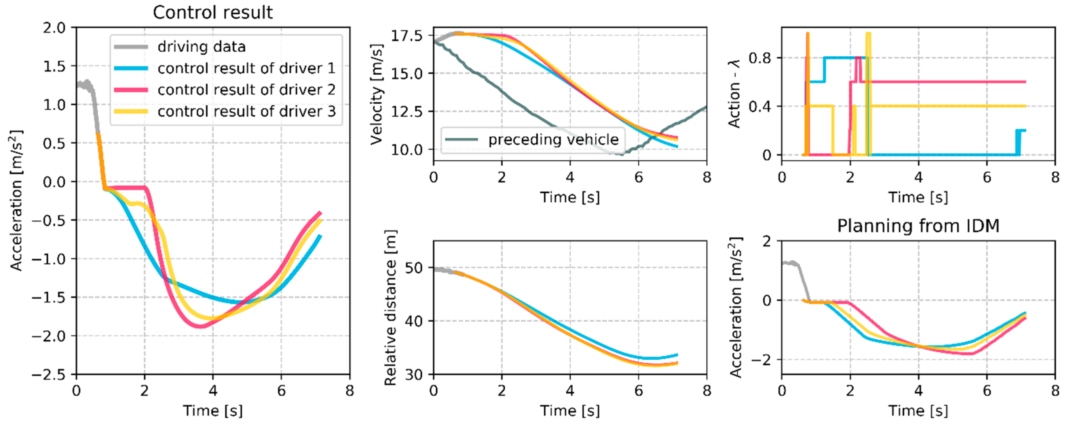
Figure 19 shows the different control results according to individual driver model at the same deceleration condition. The agent has learned using different driver parameters to reflect the driver characteristics. As a result, the control results and weight factor of planning management are different for the same deceleration condition. The agent of driver 1 selects the action of the control result that converges to the IDM based planning because the planning result of IDM is very similar to the real driving data at this deceleration case. On the other hand, the control result of driver 2 shows the agent selects the weight factor as the MPC based planning is more dominant than the IDM based planning. Since the IDM based planning which represents the driving style of driver 2 might cause the safety problem, the agent has learned to select MPC based planning at this deceleration case.
7. Conclusions
This paper proposed the SRC system based on the reinforcement learning algorithm. The proposed algorithm recognizes the deceleration condition. Then, the driver model generates the acceleration set-point using two planning methods and a planning management algorithm. The model-based planning method can represent the individual driver characteristics, and the optimization-based planning method can determine the safety speed trajectory under diverse deceleration conditions. The planning management selects the weight factor among these two planning methods.
The planning management was determined based on the reinforcement learning algorithm, which selects the optimal weight factor as an action to maximize the future cumulative reward. The proposed algorithm can determine the optimal deceleration set-point using this weight factor that considers the determined rewards about the driver intention, energy efficiency, and safety.
The proposed algorithm was learned and validated using the vehicle experiment data under various deceleration conditions. As learning results, the algorithm determined the appropriate deceleration set-point for the SRC system depending on the driving conditions. Furthermore, the algorithm can reflect the individual driver characteristics using the driver model-based planning algorithm.
Author Contributions
Conceptualization, I.P. and S.Y.; investigation, I.P.; methodology, K.M., G.S. and S.A.; software, G.S. and S.A.; supervision, K.M. and J.Y.; validation, S.Y.; writing—review & editing, K.M.
Funding
This work was financially supported by the BK21 plus program (22A20130000045) under the Ministry of Education, Republic of Korea, the Industrial Strategy Technology Development Program (No. 10039673, 10060068, 10079961), the International Collaborative Research and Development Program (N0001992) under the Ministry of Trade, Industry and Energy (MOTIE Korea), and National Research Foundation of Korea (NRF) grant funded by the Korean government (MEST) (No. 2011-0017495).
Acknowledgments
The experiment vehicle was supported by the Hyundai motor company.
Conflicts of Interest
The authors declare no conflict of interest.
References
- Balasubramanian, B.; Huzefa, A.C. Development of regeneration braking model for electric vehicle range improvement. In Proceedings of the 2017 IEEE Transportation Electrification Conference, Pune, India, 13–15 December 2017; IEEE: Piscataway, NJ, USA, 2017; pp. 1–5. [Google Scholar]
- McCall, J.C.; Trivedi, M.M. Driver Behavior and Situation-aware Brake Assistance for Intelligent Vehicles. Proc. IEEE 2007, 95, 374–387. [Google Scholar] [CrossRef]
- Hyundai UK. Discover the New Hyundai Kona Electric—Electric SUV. Available online: https://www.hyundai.co.uk/new-cars/kona-electric (accessed on 26 September 2018).
- LaValle, S.M. Planning Algorithms; Cambridge University Press: Cambridge, UK, 2006. [Google Scholar]
- Gonzalez, D.; Perez, J.; Milanes, V.; Nashashibi, F. A Review of Motion Planning Techniques for Automated Vehicles. IEEE Trans. Intell. Transp. Syst. 2016, 17, 1135–1145. [Google Scholar] [CrossRef]
- Lang, D.; Schmied, R.; Del Re, L. Prediction of Preceding Driver Behavior for Fuel Efficient Cooperative Adaptive Cruise Control. SAE Int. J. Engines 2014, 7, 14–20. [Google Scholar] [CrossRef]
- Butakov, V.A.; Ioannou, P. Personalized Driver Assistance for Signalized Intersections Using V2I Communication. IEEE Trans. Intell. Transp. Syst. 2016, 17, 1910–1919. [Google Scholar] [CrossRef]
- Li, X.; Sun, Z.; Cao, D.; He, Z.; Zhu, Q. Real-Time Trajectory Planning for Autonomous Urban Driving: Framework, Algorithms, and Verifications. IEEE/ASME Trans. Mechatron. 2016, 21, 740–753. [Google Scholar] [CrossRef]
- Nilsson, J.; Brannstrom, M.; Fredriksson, J.; Coelingh, E. Longitudinal and Lateral Control for Automated Yielding Maneuvers. IEEE Trans. Intell. Transp. Syst. 2016, 17, 1404–1414. [Google Scholar] [CrossRef]
- Ziegler, J.; Bender, P.; Dang, T.; Stiller, C. Trajectory planning for Bertha—A local, continuous method. 2014 IEEE Intelligent Vehicles Symposium Proceedings, Dearborn, MI, USA, 8–11 June 2014; pp. 450–457. [Google Scholar]
- Malinauskas, R. The Intelligent Driver Model: Analysis and Application to Adaptive Cruise Control The Intelligent Driver Model: Analysis and Application. Master’s Thesis, Clemson University, Clemson, SC, USA, May 2014. [Google Scholar]
- Min, K.; Yeon, K.; Sim, G.; Sunwoo, P.M. Prediction Algorithm for Decelerating Driving States Based on Driver Characteristics for Smart Regenerative Control of Electric Vehicles. Presented at Aachen Colloquium China, Beijing, China, 9–10 October 2018. [Google Scholar]
- Qi, X.; Luo, Y.; Wu, G.; Boriboonsomsin, K.; Barth, M.J. Deep Reinforcement Learning-Based Vehicle Energy Efficiency Autonomous Learning System. In Proceedings of the 2017 IEEE Intelligent Vehicles Symposium (IV), Los Angeles, CA, USA , 11–14 June 2017; pp. 1228–1233. [Google Scholar]
- Liessner, R.; Schroer, C.; Dietermann, A.; Bernard, B. Deep Reinforcement Learning for Advanced Energy Management of Hybrid Electric Vehicles. In Proceedings of the 10th International Conference on Agents and Artificial Intelligence, Madeira, Portugal, 16–18 January 2018; Volume 2, pp. 978–989. [Google Scholar]
- Xiong, R.; Cao, J.; Yu, Q. Reinforcement Learning-Based Real-Time Power Management for Hybrid Energy Storage System in the Plug-In Hybrid Electric Vehicle. Appl. Energy 2018, 211, 538–548. [Google Scholar] [CrossRef]
- Cao, J.; Xiong, R. Reinforcement Learning-based Real-time Energy Management for Plug-in Hybrid Electric Vehicle with Hybrid Energy Storage System. Energy Procedia 2017, 142, 1896–1901. [Google Scholar] [CrossRef]
- Chen, M.; Rincon-Mora, G.A. Accurate Electrical Battery Model Capable of Predicting Runtime and I–V Performance. IEEE Trans. Energy Convers. 2006, 21, 504–511. [Google Scholar] [CrossRef]
- Coleman, T.F.; Li, Y. On the Convergence of Interior-Reflective Newton Methods for Nonlinear Minimization Subject to Bounds. Math. Program. 1994, 67, 189–224. [Google Scholar] [CrossRef]
- Coleman, T.F.; Li, Y. An Interior Trust Region Approach for Nonlinear Minimization Subject to Bounds. SIAM J. Optim. 1996, 6, 418–445. [Google Scholar] [CrossRef]
- Chae, H.; Kang, C.M.; Kim, B.; Kim, J.; Chung, C.C.; Choi, J.W. Autonomous Braking System via Deep Reinforcement Learning. In Proceedings of the 2017 IEEE International Conference on Intelligent Transportation Systems, Yokohama, Japan, 16–19 October 2017; pp. 1–6. [Google Scholar]
- Nair, A.; Srinivasan, P.; Blackwell, S.; Alcicek, C.; Fearon, R.; De Maria, A.; Panneershelvam, V.; Suleyman, M.; Beattie, C.; Petersen, S.; et al. Massively Parallel Methods for Deep Reinforcement Learning. Presented at the Deep Learning Workshop, International Conference on Machine Learning, Lille, France, 6–11 July 2015. [Google Scholar]
- Bellman, R. A Markovian Decision Process. J. Math. Mech. 1957, 6, 679–684. [Google Scholar] [CrossRef]
- Watkins, C.J.C.H.; Dayan, P. Q-learning. Mach. Learn. 1992, 8, 279–292. [Google Scholar] [CrossRef]
- Rajamani, R. Dynamics and Control of Hybrid Gas Electric Vehicles. In Vehicle Dynamics and Control; Springer: Boston, MA, USA, 2012. [Google Scholar]
Figure 1.
Algorithm overview.
Figure 1.
Algorithm overview.
Figure 2.
Vehicle model structure.
Figure 2.
Vehicle model structure.
Figure 3.
Chen battery model.
Figure 3.
Chen battery model.
Figure 4.
Vehicle modeling results.
Figure 4.
Vehicle modeling results.
Figure 5.
Regenerative control of the vehicle model.
Figure 5.
Regenerative control of the vehicle model.
Figure 6.
Driver model parameters and deceleration profile.
Figure 6.
Driver model parameters and deceleration profile.
Figure 7.
Model prediction process.
Figure 7.
Model prediction process.
Figure 8.
Model parameters and its updated vector for each driver.
Figure 8.
Model parameters and its updated vector for each driver.
Figure 9.
Deceleration planning results according to the individual driver.
Figure 9.
Deceleration planning results according to the individual driver.
Figure 10.
Deceleration planning results according to N weight value (qdf: 0.1, qvf: 4).
Figure 10.
Deceleration planning results according to N weight value (qdf: 0.1, qvf: 4).
Figure 11.
Deceleration planning results according to qdf weight value (N: 15, qvf: 0.1).
Figure 11.
Deceleration planning results according to qdf weight value (N: 15, qvf: 0.1).
Figure 12.
Deceleration planning results according to qvf weight value (N: 15, qdf: 4).
Figure 12.
Deceleration planning results according to qvf weight value (N: 15, qdf: 4).
Figure 13.
Reinforcement learning for torque control management.
Figure 13.
Reinforcement learning for torque control management.
Figure 14.
RNN architecture with LSTM cell.
Figure 14.
RNN architecture with LSTM cell.
Figure 15.
Learning and Regenerative control results for deceleration case.
Figure 15.
Learning and Regenerative control results for deceleration case.
Figure 16.
Velocity control results based on the various planning algorithms.
Figure 16.
Velocity control results based on the various planning algorithms.
Figure 17.
Regeneration control results using driving data.
Figure 17.
Regeneration control results using driving data.
Figure 18.
Validation results under various deceleration cases.
Figure 18.
Validation results under various deceleration cases.
Figure 19.
Regenerative control results depending on the individual driver.
Figure 19.
Regenerative control results depending on the individual driver.
Table 1.
Vehicle model parameters.
Table 1.
Vehicle model parameters.
| Symbol | Description | Value [unit] | Symbol | Description | Value [unit] |
|---|
| Vehicle acceleration | [m/s2] | | Inertia of wheel | 0.14 [khm2] |
| Vehicle velocity | [m/s] | | Inertia of motor | 0.028 [khm2] |
| Motor torque | [Nm] | | Inertia of shaft | 0.75 [khm2] |
| Drag force | [N] | | Air drag coefficient | 0.171 [Ns2/m2] |
| Wheel radius | 0.318 [m] | | Rolling coefficient | 143 [N] |
| Gear ratio of shaft | 7.98 [−] | | Rolling coefficient | 0.389 [Ns2/m2] |
| Efficiency of shaft | 0.99 [−] | | Additional mass | 100 [kg] |
| Empty vehicle mass | 1685 [kg] | | | |
Table 2.
Battery model parameters.
Table 2.
Battery model parameters.
| Symbol | Description | Value [unit] | Symbol | Description | Value [unit] |
|---|
| Series register | 0.0016 [Ohm] | | Short capacitor param a | −649 |
| Short register param a | 76.52 | | Short capacitor param b | −64.3 |
| Short register param b | −7.95 | | Short capacitor param c | 12,692 |
| Short register param c | 23.83 | | Long capacitor param a | −78,409 |
| Long register param a | 5.21 | | Long capacitor param b | −0.013 |
| Long register param b | −35.23 | | Long capacitor param c | 30,802 |
| Long register param c | 124.9 | | Open circuit voltage | 356 [V] |
Table 3.
MPC model for deceleration planning.
Table 3.
MPC model for deceleration planning.
| | | | |
|---|
| | | | |
© 2019 by the authors. Licensee MDPI, Basel, Switzerland. This article is an open access article distributed under the terms and conditions of the Creative Commons Attribution (CC BY) license (http://creativecommons.org/licenses/by/4.0/).
