Model Retraining upon Concept Drift Detection in Network Traffic Big Data

Abstract

This paper presents a comprehensive model for detecting and addressing concept drift in network security data using the Isolation Forest algorithm. The approach leverages Isolation Forest’s inherent ability to efficiently isolate anomalies in high-dimensional data, making it suitable for adapting to shifting data distributions in dynamic environments.Anomalies in network attack data may not occur in large numbers, so it is important to be able to detect anomalies even with small batch sizes. The novelty of this work lies in successfully detecting anomalies even with small batch sizes and identifying the point at which incremental retraining needs to be started. Triggering retraining early also keeps the model in sync with the latest data, reducing the chance for attacks to be successfully conducted. Our methodology implements an end-to-end workflow that continuously monitors incoming data and detects distribution changes using Isolation Forest, then manages model retraining using Random Forest to maintain optimal performance. We evaluate our approach using UWF-ZeekDataFall22, a newly created dataset that analyzes Zeek’s Connection Logs collected through Security Onion 2 network security monitor and labeled using the MITRE ATT&CK framework. Incremental as well as full retraining are analyzed using Random Forest. There was a steady increase in the model’s performance with incremental retraining and a positive impact on the model’s performance with full model retraining.

1. Introduction and Background

Machine learning models learn from data and make predictions. But in today’s fast evolving network traffic environment, what a machine learner learned in the past might not work with newer data or attacks. Real-world machine learning applications must learn to handle data that evolves over time, and this is the challenge we address in this paper using the idea of concept or data drift. Concept or data drift happens when a machine learner is trying to predict or understand “something” that starts to change over time [1]. Hence, this research addresses the critical challenge of maintaining effective anomaly detection systems in dynamic network environments where the nature of both normal and malicious activities continuously evolves. This evolution can occur due to evolving trends or other factors that cause data to shift over time. In the rapidly evolving landscape of network security, concept drift presents a significant challenge to maintaining effective anomaly detection systems when attacks are sporadically changing over time.

Isolation Forest is a machine learning algorithm often used for anomaly detection. It works by isolating anomalies or “outliers” in the data rather than modeling normal data points. The key idea is that anomalies are rare and different, so they can be isolated with fewer steps compared to normal data points. The benefits of using Isolation Forest are that it is efficient with high-dimensional data [2,3]. Its speed and scalability, stemming from simpler calculations [4], make it well-suited for Big Data. It does not rely on complex calculations and works well with large datasets [4]. It specifically targets anomalies which are isolated quickly due to their rarity and distinctness. This makes it highly effective for detecting anomalies [2,3].

By combining Isolation Forest’s efficient anomaly detection using drift detection and Random Forest’s retraining mechanisms, we provide a robust solution for modern network security challenges. This framework not only employs Isolation Forest for efficient anomaly detection but also integrates automated drift detection and retraining mechanisms. Two types of retraining are analyzed using Random Forest, incremental retraining and full retraining. Incremental retraining is started as soon as the data drift is identified. In real-world scenarios, anomalies, in this case network attacks, may not come in large numbers, so it is important to be able to detect anomalies even with small batch sizes. Leveraging the fact that Isolation Forest works well even when the sampling size is kept small [4], the novelty of this work lies in successfully being able to detect anomalies even with small batch sizes, even when the attacks may be sporadic, and detecting the point at which incremental retraining needs to be started. Triggering retraining early keeps the model in sync with the latest data, reducing the chance for attacks to be successfully conducted.

By systematically identifying concept drift and dynamically updating the model, we enhance the adaptability and robustness, ensuring that the model remains effective in detecting threats despite shifting data patterns. By leveraging PySpark’s processing capabilities, we efficiently handle Big Data. This framework significantly improves the resilience of network security systems against evolving cyber threats by providing a proactive rather than reactive approach to anomaly detection and concept drift adaptation.

The rest of this paper is organized as follows: Section 2 presents the related works in terms of traditional drift detection methods, concept drift, machine learning, the Isolation Forest algorithm, and model retraining strategies; Section 3 presents the data and processing; Section 4 presents the algorithms and evaluation metrics used; Section 5 presents the experimentation as well as the results and discussion of the results; Section 6 presents the conclusions; and finally, Section 7 presents future work.

2. Related Works

Since this work would not be successful without introducing several concepts, this section addresses traditional drift detection methods, concept drift in machine learning, the Isolation Forest algorithm, model retraining strategies, and finally, the gaps in the literature that will be covered by this study.

2.1. Traditional Drift Detection Methods

The field of drift detection has evolved significantly, with various approaches developed to address different aspects of the challenge. Statistical-based methods form the foundation of many drift detection approaches. Page (1954) [5] introduced the Cumulative Sum charts, which remain relevant for detecting sustained shifts in data distributions. Hinkley (1971) [6] further developed these concepts with the Page–Hinkley Test, while Ross adapted Statistical Process Control methods for drift detection in modern applications [7].

Performance-based methods emerged as a practical alternative, focusing on model behavior rather than raw data statistics. Gama et al. (2014) [8] monitored error rates to identify potential drift points. Baena-García et al. (2006) [9] enhanced this approach with the Early Drift Detection Method, improving sensitivity to gradual changes. The Adaptive Windowing (ADWIN) technique, introduced by Bifet and Gavalda (2007) [10], provided a flexible framework for handling variable-speed drift scenarios. In contrast, our work will base drift detection on a statistical measure, the drift factor, which is based on the anomaly rate.

2.2. Concept Drift in Machine Learning

In machine learning applications, concept drift represents a fundamental challenge where the statistical properties of the target variable evolve over time in unpredictable ways. Gama et al. (2014) [8] formally defined this phenomenon, noting that such changes can significantly impact model accuracy and reliability over time. The literature identifies several distinct types of concept drift, each presenting unique challenges for detection and adaptation systems.

Sudden drift, as described by Webb et al. (2016) [11], occurs when the underlying concept changes abruptly. This type of drift is particularly challenging in network security contexts, where rapid shifts in attack patterns can render existing detection models obsolete almost instantly. In contrast, gradual drifts represent a subtler evolution of patterns, where new concepts slowly replace old ones over time. Žliobaitė et al. (2016) [12] demonstrated how such gradual changes often reflect natural evolution in system behaviors and user patterns. Additionally, Barros et al. (2018) [13] identified recurring drift patterns, where certain concepts periodically disappear and reappear.

2.3. Isolation Forest Algorithm

The Isolation Forest algorithm represents a significant advancement in anomaly detection, particularly suited for concept drift scenarios. Liu et al. (2008) [4] introduced this approach, demonstrating its unique ability to identify anomalies through isolation rather than density estimation. The algorithm’s efficiency stems from its tree-based structure, which naturally handles high-dimensional data while maintaining linear time complexity.

Recent work by Ding and Fei (2013) [14] has shown how Isolation Forest’s characteristics make it particularly effective for streaming data environments. The algorithm’s ability to operate with partial models and its efficient sub-sampling capabilities provide significant advantages for real-time applications. Togbe et al. (2021) [15] further demonstrated its robustness in handling evolving data patterns, while Xu et al. (2023) [16] showed its effectiveness in detecting both gradual and sudden drift patterns. Our work does not really look at whether a drift is gradual or sudden; this work just determines any drift, be it gradual or sudden. Given that our data deals with attacks in network traffic data, the drift could be gradual or sudden.

2.4. Model Retraining Strategies

Effective model retraining strategies are crucial for maintaining system performance in the presence of concept drift. Krawczyk et al. (2017) [17] explored full retraining approaches, which, while computationally intensive, provide comprehensive model updates. Losing et al. (2018) [18] investigated incremental learning methods, offering more efficient updates but potentially suffering from error accumulation over time. Lu et al. (2018) [19] proposed hybrid approaches that balance computational efficiency with model accuracy, adapting the retraining strategy based on drift severity and pattern characteristics.

2.5. Research Gaps and Challenges

Despite significant advances in drift detection and adaptation, several challenges persist. Barros et al. (2018) [13] highlighted the critical trade-off between detection speed and false alarm rates, particularly in security-sensitive applications. Webb et al. (2018) [11] addressed the challenge of maintaining model stability while ensuring adaptability to new patterns. These challenges become particularly acute in network security applications, where both false positives and missed detections can have significant consequences.

To differentiate this paper from previous works, it is important to note that earlier studies presented theoretical improvements to algorithms and demonstrated results on benchmark datasets. In contrast, this paper’s unique contributions lie in demonstrating how incremental versus full retraining behave, especially when small batch sizes are used.

3. Data and Preprocessing

The Zeek Conn Log MITRE ATT&CK framework-labeled dataset [20], UWF-ZeekDataFall22 [21], available at [22], generated using the Cyber Range at the University of West Florida (UWF), was used for this analysis. The MITRE ATT&CK framework [18] is a modern set of adversary tactics and techniques based on real-world attacks. Presently the MITRE ATT&CK framework has 14 tactics and several techniques under each tactic. Techniques represent how an adversary achieves a tactical goal by performing an action.

Figure 1 presents a breakdown of the Zeek Conn Log MITRE ATT&CK techniques present in UWF-ZeekDataFall22 [21]. Each technique is described in Appendix A [20].

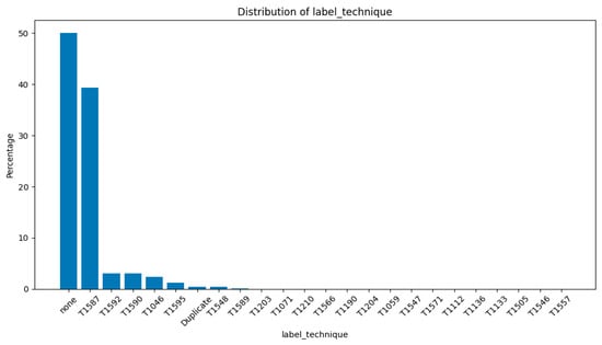
Figure 1. Distribution of label techniques in UWF-ZeekDataFall22.

3.1. Dataset Overview

This dataset comprises 700,340 records of structured network traffic with 25 distinct features [23], spanning multiple days. The dataset represents network traffic patterns with both normal and anomalous behavior, providing a comprehensive base for concept drift detection. Figure 2 shows the distribution of events by the hour of a day in the UWF-ZeekDataFall22 dataset.

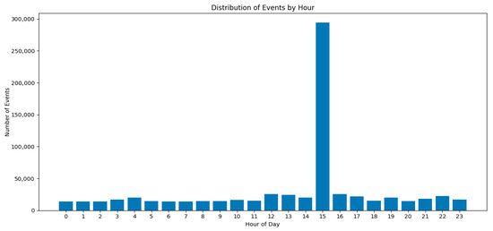
Figure 2. Distribution of events by hour.

3.2. Data Preprocessing

In terms of data preprocessing, the following was performed:

(i)

first, columns that were deemed irrelevant to the study (community_id, ts (timestamp)) were dropped;

(ii)

duplicate rows were dropped;

(iii)

to assess the data quality, the missing values were analyzed;

(iv)

the data distribution was determined, mainly to help us determine if numerical features would have to be binned; and finally,

(v)

the data was binned.

3.2.1. Missing Values Analysis

Table 1 presents a missing value analysis for the features that have missing values. Count is the number of records and percentage is the percent of the total dataset.

Table 1. Missing Values Analysis.

Feature	Count	Percentage
Duration	317,051	45.30%
Service	317,407	45.30%
History	8206	1.20%

For Service and History, the missing values formed a category of their own called “Blanks”, and for Duration, the missing values were replaced with the average.

3.2.2. Data Distribution

Table 2 presents the range of values for each of the numeric features. Duration is presented in seconds; the source and destination ports are the range of port numbers for the source and destinations, respectively; and the original and response bytes are the number of bytes being transferred.

Table 2. Range of numeric features.

Features	Range
Duration (seconds)	0 to 3560
Source Ports	0 to 65,535
Destination Ports	0 to 65,535
Original Bytes	0 to 218,820
Response Bytes	0 to 2,174,312
…	…

3.2.3. Binning the Data

Continuous features, especially features with a wide range of values, were binned into discrete categorical intervals. Features with too many less significant counts in certain categories were grouped or binned into fewer, more manageable categories.

As presented in Table 3, UWF-ZeekDataFall22 has mainly five different tactics: Resource Development, Reconnaissance, Discovery, Privilege Escalation, and Defense Evasion. Tactics that were very low in numbers were grouped into the “Other” category.

Table 3. Distribution and binning of tactics.

Tactics	Binned Value	Definition	Distribution
None	0	Benign data	50.02%
Resource Development	1	Tactic involves an adversary setting up resources to maintain access and advance their attack [24]	39.33%
Reconnaissance	2	The process of collecting initial information or intelligence about a target [25]	7.35%
Discovery	3	Adversary will seek information on the system [26]	2.40%
Privilege Escalation	4	Tactic involving various techniques adversaries use to gain higher-level permissions within a system or network [27]	0.44%
Defense Evasion	5	Uses methods to avoid being detected [28]	0.44%
Other Categories	6	Includes the following: Lateral Movement, Execution, Command and Control, Persistence, Collection, and Initial Access [20]	0.02%

Table 4 and Table 5 display the distribution and binning of the protocol and service features, respectively. Protocol is the transport layer protocol of the connection and service is the identification of the application protocol being sent over the connection [23].

Table 4. Distribution and binning of protocol.

Protocols	Binned Value	Distribution
UDP	0	55.47% (388,470 records)
TCP	1	44.39% (310,910 records)
ICMP	2	0.14% (960 records)

Table 5. Distribution and binning of service.

Service	Binned Value	Count
dns	0	381,896
dhcp	2	633
http	3	168
ntp	4	169
ssl	5	37
radius	6	1
gssapi	7	5
smb,gssapi	8	4
dce_rpc,smb,gssapi,ntlm	9	1
ftp	10	5
gssapi,smb,dce_rpc,ntlm	11	3
ntlm,smb,gssapi	12	3
smb,ntlm,gssapi	13	1
snmp	14	3
gssapi,smb	15	1
gssapi,smb,ntlm	16	2
ntlm,gssapi,dce_rpc,smb	17	1
(blanks)	18	317,407

Table 6 presents the binning performed of IP addresses and ports. The IP address columns, src_ip_zeek, dest_ip_zeek, were categorized into the following: “Private”, “Public”, “Special”, or “Invalid”, as per [29].

Table 6. Distribution and binning of IP addresses.

Category	IP Address
Invalid IP
Private (RFC 1918)	Class A 10.0.0.0/8
Private (RFC 1918)	Class B 172.16.0.0/12
Private (RFC 1918)	Class C 192.168.0.0/16
Public IP	Known Services (80, 443, etc.)
Public IP	Other
Localhost	127.0.0.0/8
Link-local	169.254.0.0/16
Special	Multicast, Reserved (RFC 6890)

As presented in Table 7, the ports features src_port_zeek and dest_port_zeek were categorized into the following: “Well-known”, “Registered”, “Dynamic”, or “Invalid”, as per [30]. The connection state, conn_state, was binned, as presented in Table 8.

Table 7. Distribution and binning of ports.

Category	Port Range
Well Known	1–1023
Registered	1024–49,151
Dynamic	49,152–65,535
Invalid	0 or none

Table 8. Distribution and binning of conn_state.

Conn_State	Binned Value	Count
S0	0	587,615
SF	1	75,749
SHR	2	5249
OTH	3	9897
SH	4	20,682
RSTRH	5	338
REJ	6	306
RSTR	7	300
RSTO	8	158
S1	9	39
S2	10	7

The source and response bytes, which were continuous numerical data, were converted into discrete categorical intervals, as presented in Table 9.

Table 9. Distribution and binning of bytes.

No Data	0 Bytes	Explanation
Tiny	1–50 bytes	Typically control packets
Small	51–100 bytes	Small requests/responses
Medium	101–500 bytes	Typical web requests
Large	501–1000 bytes	Larger requests/responses
Very Large	1001–10,000 bytes	File transfers
Huge	>10,000 bytes	Large file transfers

4. Algorithms and Evaluation Metrics Used

4.1. Random Forest

Random Forest is an ensemble machine learning algorithm that combines multiple decision trees for improved prediction accuracy. Each tree in the forest is built using a random subset of both the training data and features. During prediction, each tree independently evaluates the input and produces its own result. For classification problems, the final output is determined by majority voting across all trees, while for regression problems, it averages all tree predictions. This approach of combining randomized trees helps reduce overfitting and handles both numerical and categorical data effectively, making Random Forest a versatile and robust algorithm for various machine learning classification [31,32].

Evaluating Random Forest

Accuracy measures the overall true correct predictions out of the total predictions in the model. It gives a quick overall sense of how well the model performs. A high accuracy means the model is functioning well while a low accuracy indicates that the data may need to be updated [33].

$$Accuracy={\displaystyle \frac{(True Positives+True Negatives)}{(True Positives+True Negatives+False Positives+False Negatives)}}$$

(1)

Precision reflects the amount of data that was predicted to be an anomaly that were actually anomalies. Calculating precision allows us to avoid false alarms and build trust in the model [34].

$$Precision={\displaystyle \frac{(True Positives)}{(True Positives+False Positives)}}$$

(2)

Recall identifies how many actual anomalies were correctly identified. Recall (also known as Sensitivity or True Positive Rate) measures how well the model identifies all actual positive cases [34]. Precision focuses on the quality of the positive predictions while recall focuses on the completeness.

$$Recall={\displaystyle \frac{(True Positives)}{(True Positives+False Negative)}}$$

(3)

The F1 score is a balanced measure that combines precision and recall. It provides a single score that balances both the precision and the recall of a model [34].

$$F1 Score={\displaystyle \frac{(Precision\times Recall)}{(Precision+Recall)}}$$

(4)

The Confusion Matrix summarizes the performance of a classification model. It shows the counts of correct and incorrect predictions made by the model, broken down by each class. The matrix typically consists of four key components:

• True Positive (TP): The number of cases where the model correctly predicted the positive class.
• True Negative (TN): The number of cases where the model correctly predicted the negative class.
• False Positive (FP): The number of cases where the model incorrectly predicted the positive class when it was actually negative. This is also known as a Type I error.
• False Negative (FN): The number of cases where the model incorrectly predicted the negative class when it was actually positive. This is also known as a Type II error.

4.2. Isolation Forest

Isolation Forest is an anomaly detection algorithm that, like Random Forest, utilizes an ensemble of decision trees, but with a distinct purpose and methodology. It operates on the principle that anomalies are easier to isolate than normal data points, requiring fewer random partitions to separate them from the rest of the data. Unlike traditional methods, Isolation Forest does not require building a profile of normal behavior or density estimation, making it computationally efficient. The algorithm works by randomly selecting features and splits points to create isolation trees, recording the path length required to isolate each data point. It then assigns anomaly scores based on average path lengths across multiple trees, with shorter paths indicating likely anomalies and longer paths suggesting normal observations [5].

The anomaly score is a value between 0 and 1, where scores closer to 1 indicate a higher likelihood of being an anomaly. Typically, a threshold is used to make the final determination—points with scores above this threshold are flagged as anomalies. In practice, these scores can be used to trigger various actions in a monitoring system. For example, if the proportion of detected anomalies exceeds a predetermined threshold, this could trigger a model retraining process. Additionally, the nature of the detected anomalies can provide insights into potential data drift or concept drift, where the underlying patterns in the data have changed significantly from the training data [5]. Isolation Forest’s unsupervised nature also means it can potentially identify novel types of anomalies that might be missed by supervised methods trained on historical data [5].

In this work, concept drift is measured by tracking shifts in anomaly detection rates. To quantify the severity of the drift, changes in the anomaly score distributions between the baseline and drifted datasets are studied. A significant increase in detected anomalies indicates potential drift.

Identifying Concept Drift

To validate concept drift detection, Isolation Forest’s performance on the drifted test dataset was compared against its performance on the baseline test set. Changes in anomaly rates and variations in prediction confidence were analyzed to confirm the presence of concept drift and assess the model’s robustness against subtle and substantial anomalies. The formulas for the Base Anomaly Rate, New Anomaly Rate, and Drift Factor are in Equations (5), (6), and (7), respectively.

$$Baseline Anomaly Rate={\displaystyle \frac{\# of anomalies in Original Test Data}{Total \# of Instances in Original Test Data}}$$

(5)

$$New Anomaly Rate={\displaystyle \frac{\# of New Anomalies}{Total \# of instances in New Test Data}}$$

(6)

$$Drift Factor={\displaystyle \frac{New Anomaly Rate}{Baseline Anomaly Rate}}$$

(7)

5. Experimentation Including the Results and Discussion

5.1. Framework for Concept Drift Detection

This model implements an end-to-end pipeline for detecting concept drift and retraining the model. As shown in Figure 3, the system consists of the following key stages:

• Splitting data into training and testing sets;
• Training an initial model and recording baseline performance;
• Processing new data in batches;
• Detecting drift based on changes in anomaly rates derived from Isolation Forest output;
• Retraining the model upon significant drift detection;
• Validating the retrained model’s performance.

Each stage of Figure 3 is detailed out in Figure 4a–d. Figure 5 presents a components diagram that presents all the components that were used in various phases of Figure 3 (or Figure 4a–d).

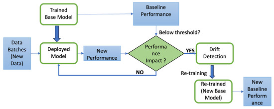
Figure 3. System diagram for training/retraining data.

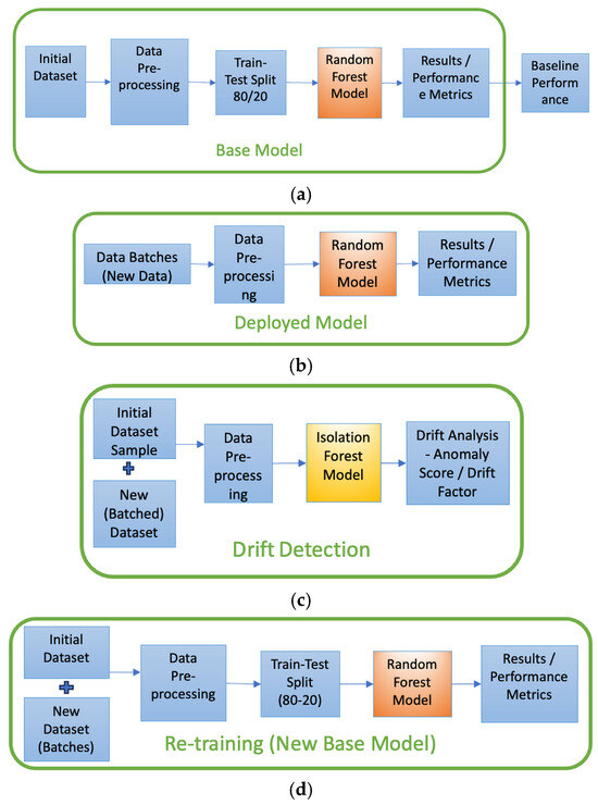
Figure 4. (a) Base Model, (b) Deployed Model, (c) Drift Detection, (d) Re-training (New Base Model).

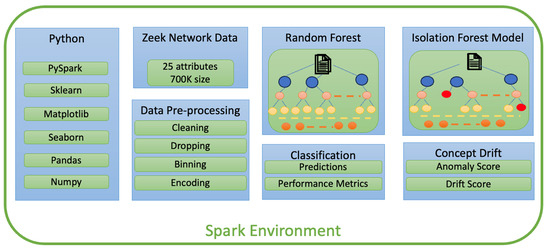
Figure 5. Components diagram.

5.2. Experimental Configurations Utilized

This section provides the hardware and software specifications as well as the parameters/hyperparameters used in this experimentation.

5.2.1. Hardware Specifications

This experiment was conducted using the following hardware configurations: a multi-core CPU processor with 8 cores, 16 GB of RAM, and 10 GB of SSD.

5.2.2. Software Specifications

The software specifications are as follows:

• Apache Spark;
• Isolation Forest (from scikit-learn);
• Mac/Ubuntu OS.

With core dependencies:

○

Python: 3.6;

○

PySpark: 3.0.0;

○

NumPy: 1.19.0;

○

pandas: 1.2.0;

○

scikit-learn: 0.24.0;

○

matplotlib: 3.3.0;

○

seaborn: ≥0.11.0.

5.2.3. Parameters/Hyperparameters

After extensive experimentation, the following parameters/hyperparameters were finally used.

Core Isolation Forest Parameters:

○

Contamination, which is the expected proportion of anomalies in the dataset, was kept at 0.01;

○

n_estimators, which is the number of base estimators (trees) n the ensemble, was kept at 100;

○

n_jobs, which is the number of parallel jobs to run for model training/testing, was kept at 1;

○

num_iterations, which is the number of times the Isolation Forest algorithm runs with different samples, was kept at 2.

Data Processing Parameters:

○

sample_fraction, which is the fraction of data to sample for each Isolation Forest run, was kept at 0.01;

○

variance_threshold, which is the threshold for feature selection based on variance, was kept at 0.01;

○

confidence_threshold, which is the threshold for considering an anomaly as high confidence, was kept at 0.7

5.3. Developing the Base Model

As shown in Figure 3, we start with developing the base model (shown in Figure 4a), which is used for comparison. After data preprocessing, the data is split into training/testing (80%/20%, respectively) and, to determine if concept drift could be detected in this dataset, UWF-ZeekDataFall22, some of the testing data was kept aside to test as new batch data. The new batches would be used to see if a concept drift was occurring and if this could be detected.

The model was then trained with the training data using Random Forest, and the testing was performed with part of the testing data. The testing data was randomly selected from the 20% testing data and inserted in batches after inserting some attack data. The idea when generating the batches was to simulate the early detection of anomalies, that is, to make the model more sensitive, hence triggering incremental retraining as early as possible when a drift is detected. Batch sizes affect how quickly the model adapts. Smaller, more frequent batches allow for more responsive adaptation, hence smaller batch sizes were used.

To generate the batches, a Fibonacci sequence was generated and normalized to percentages. These percentages would determine the proportion of “used” (data the model was trained on) to “unused” (new data the model has not seen) data in each batch. Also added to the test data were attacks, a randomly picked percentage from the different attack groups to simulate the sporadic nature of attacks. Since the number of attacks in the attack groups are different, the batches are also different in count.

The model’s performance was evaluated through multiple metrics, as presented in Table 10, which presents the base model’s accuracy, precision, recall, and F1-score for both the training as well as testing datasets. Table 10 also presents the total run times for training as well as testing. The nearly identical values across training and testing indicate that the model generalizes well and is not overfitting. These results provide a baseline against which a drift can be detected.

Table 10. Model performance metrics: training vs. testing data (baseline results).

	Total Records	Accuracy	Precision	Recall	F1-Score	Total Time (s)
Training	534,365	98.99%	98.99%	98.99%	98.99%
Testing	134,398	98.95%	98.95%	98.95%	98.95%
						1271.84

5.4. Deploying the Model

As per Figure 4b, once the model has been trained and tested, to detect potential drift, small batches of new data are inserted. The amount of data inserted in each batch is presented in Table 11. Most models require large amounts of data, but Isolation Forest works well even when the small sizes are small [6]. In fact, contrary to general machine learning models, large amounts of data often reduces Isolation Forest’s ability to isolate anomalies as normal instances can mask Isolation Forest’s ability to isolate anomalies [6]; hence, small batch sizes of new data were used.

Table 11. Detecting concept drift: performance metrics before retraining.

Batch	Total Records	Accuracy	Precision	Recall	F1	FN	TP	TN	FP	Run Times (s)
1	213	92.49%	0.9941	91.85%	95.48%	18	148	36	0	10.78
2	146	89.73%	100%	88.28%	93.78%	12	97	21	1	7.68
3	116	90.52%	100%	89.52%	94.47%	14	66	7	0	7.66
4	88	87.50%	100%	86.08%	92.52%	7	58	5	0	7.39
5	71	90.14%	100%	89.06%	94.21%	16	52	8	0	7.63
6	58	81.03%	100%	80.36%	89.11%	12	52	3	0	7.21
7	76	78.95%	100%	78.67%	88.06%	17	49	2	0	6.22
8	97	79.38%	100%	79.38%	88.51%	36	74	0	0	7.05
9	119	78.99%	100%	78.99%	88.27%	50	109	1	0	6.49
10	156	73.72%	100%	73.38%	84.64%	58	118	2	0	5.89
Averages		84.25%	99.94%	83.56%	90.91%

The techniques presented in Figure 1 were randomly spread throughout the batches, simulating the sporadic nature of attacks. Very small batch sizes could lead to false positives, while overly large batches might delay drift detection. Each new data batch is evaluated against the trained model, and performance metrics are recorded. As can be seen from the results in Table 11, as new data is being added, the accuracy and other metrics, precision, recall, and F1-Score, are decreasing. Additionally, the rate of false positives and false negatives were analyzed using confusion matrices. With the first batch, the accuracy was at 92.49%. With the insertion of the second batch of data, the accuracy dropped to 89.73%, and so on. And finally, with the insertion of batch 10, the accuracy was at 73.72%. There was clearly a concept drift even with very small batch sizes. The smaller batch sizes also attest to the fact that our model is highly sensitive to drift, and stronger security systems should in fact have higher sensitivity to detecting drift. In real-world scenarios, attacks will often not come in large numbers.

5.5. Drift Detection

As shown in Figure 4c, as the data starts drifting, the Isolation Forest algorithm is used to identify changes in the data distribution that might impact the model’s performance. Isolation Forest does this by detecting anomalies in new incoming data by calculating drift metrics. This is performed by tracking changes in anomaly scores across the different batches and determining if a drift occurred.

The Baseline Anomaly Rate, New Anomaly Rate, and Drift Factor, that is, Equations (5), (6), and (7), respectively, play a crucial role in determining what would be considered a concept drift in a model. The Baseline Anomaly Rate (Equation (5)), which is the number of anomalies in the original test data to the total number of instances in the test data, establishes a reference point. That is, anything higher than the Baseline Anomaly Rate would be considered anomalous data. As presented in Table 12, in this work, the baseline anomaly rate was set to 0.03 in all batches. This rate tells the model that 0.03 or 3% of all records are allowed to be anomalous. The usual standard used for a baseline anomaly rate is between 0.01 and 0.05. A higher rate leads to missing alerts, and a lower rate leads to overwhelming the alerts for the security system; 0.03 falls right in the middle.

Table 12. Concept drift evaluation (before retraining).

Batch Number	Baseline Anomaly Rate	Anomaly Score	New Anomaly Rate	Drift Factor
1	0.03	0.695162946	0.028173105	0.9391035
2	0.03	0.699885789	0.057822131	1.92740436
3	0.03	0.713253628	0.087895827	2.92986091
4	0.03	0.687121205	0.118933493	3.96444977
5	0.03	0.70820591	0.146855251	4.89517504
6	0.03	0.694885641	0.179279279	5.97597598
7	0.03	0.704640135	0.209580838	6.98602794
8	0.03	0.700928723	0.238491238	7.94970795
9	0.03	0.68240109	0.268608414	8.95361381
10	0.03	0.701152359	0.298250729	9.94169096

The New Anomaly Rate (Equation (6)) captures the proportion of new anomalies to the total number of instances in the updated test data. As shown in Table 12, the new anomaly rate steadily grows with each new batch, indicating that the nature of the data is changing. If the new anomaly rate surpasses the baseline anomaly rate of 0.03, this signals that the model is seeing more unfamiliar patterns. This will trigger retraining.

The Drift Factor (Equation (7)), which compares these two rates, the new anomaly rate to the baseline anomaly rate, determines the severity of the drift and its influence on the model’s effectiveness. The drift factor growing significantly per batch shows that each new batch is progressively different from the training data. If the drift factor exceeds the predefined threshold, set to two in this work, this would indicate a “drift-alert”, signaling that retraining needs to occur. A higher drift factor threshold would mean missing out on anomalies. A Drift Factor of 2 would indicate that the new anomaly rate is twice the baseline anomaly rate. However, an appropriate threshold is purely dependent on expectations and could vary from application to application. In Table 12, by batch 2, the Drift Factor is below 2; therefore, retraining started at batch 3.

5.6. Retraining the Model

As observed in Table 11 and Figure 6, as newer data with a higher proportion of anomalies is introduced, the model’s accuracy, recall, and F1-score begin to decline. This degradation indicates that the existing model is becoming less effective at distinguishing between normal and anomalous patterns. To quantify this decline, we identified a threshold at which retraining becomes necessary and tracked performance metrics across multiple batches. When significant drift was detected, model retraining was triggered. Retraining the model is elaborated in Figure 4d. The model was retrained using updated data, that is, by expanding the training dataset with new data.

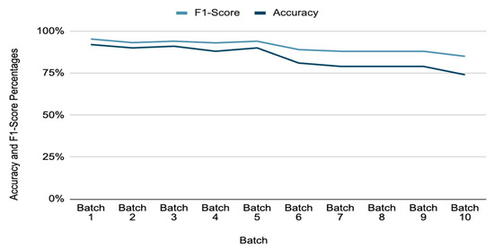
Figure 6. F1-score and accuracy before retraining.

With reference to Table 13, to evaluate batch ‘N’, the model would be trained on (Initial Training data + Batch1 data + … + Batch N-1 data). This would update the model parameters and track performance improvements. To validate the performance, the newly trained model is tested against upcoming batches and compared with previous results. Performance validation ensures that the retraining enhances predictive accuracy.

Table 13. Performance metrics after incremental retraining.

Batch	Total Records	Accuracy	Precision	Recall	F1- Score	FN	FP	TN	FP	Run Times (s)
1	213	91.58%	100%	89.76%	94.60%	17	149	36	0	10.90
2	146	87.02%	99%	85.32%	91.63%	16	93	21	1	7.91
3 *	116	85.05%	100%	83.75%	91.16%	13	67	7	0	7.25
4	88	87.14%	100%	86.15%	92.56%	9	56	5	0	7.30
5	71	88.16%	100%	86.76%	92.91%	9	59	8	0	7.84
6	58	91.04%	100%	90.63%	95.08%	6	58	3	0	7.67
7	76	92.65%	100%	92.42%	96.06%	5	61	2	0	6.27
8	97	90.91%	100%	90.91%	95.24%	10	100	0	0	7.19
9	119	95.63%	100%	95.60%	97.75%	7	152	1	0	6.76
10	156	95.51%	100%	95.45%	97.67%	8	168	2	0	6.08
Averages		90.47%	99.90%	89.68%	94.47%

* Incremental retraining starts.

As per Table 12, since a drift was detected in batch 2, batches 1 and 2 in Table 13 do not reflect results of retraining. In Table 13, retraining was started at batch 3, and Table 13 presents the results of batches 1 and 2 and the rest of the batches after retraining. As can be observed in Table 13, overall, the accuracy improves across all batches after retraining; precision remains high, near 100%, as false positives are well controlled. Recall also improves, indicating that the retrained model is better at identifying positive cases. The F1-score improves, showing a better balance between precision and recall. True positives increase, which means that more anomalies are actually being caught. False negatives remain low, meaning fewer anomalies are missed. Figure 7 presents the trends in accuracy before and after training.

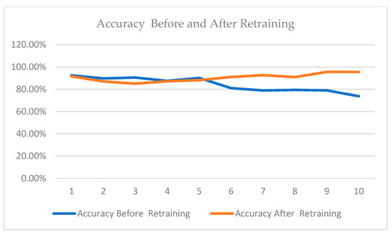
Figure 7. Accuracy before and after retraining.

5.6.1. Testing Statistical Significance

To test the statistical significance, the Z-test was used. Any two proportions can be statistically tested for significance using the Z-test. The formula for the Z-test statistic is provided by the following:

$$\mathit{Z}=({\hat{p}}_1-{\hat{p}}_2)/\sqrt{{\hat{p}}_1(1-{\hat{p}}_1)/n_1+{\hat{p}}_2(1-{\hat{p}}_2)/n_2}$$

(8)

where ${\hat{p}}_i$ denotes the estimated i-th proportion, along with the corresponding sample size, $n_i$, $i=1,2$ for this estimation. Any Z-value greater than the threshold value $z_{0.025}=1.96$ confirms the significant difference between the two proportions at a 95% confidence level.

To test if there was a significant statistical difference in the accuracy before and after retraining, the Z-test was used. As demonstrated in Table 14, the Z-values before and after retraining were significantly different. After retraining, the accuracy was significantly higher. After batch 3, the Z-value started falling, so retraining was triggered, which resulted in a significant improvement in the statistical metrics. The positive Z-value means that the first value was significantly higher than the second value and the negative Z-value means that the second value was significantly higher than the first value.

Table 14. Z-value before and after retraining.

	Accuracy Before Retraining	Accuracy After Retraining	Z-Value
1	0.9249	0.9158	8.720846
2	0.8973	0.8702	21.94895
3	0.9052	0.8505	43.47297
4	0.875	0.8714	2.805536
5	0.9014	0.8816	16.51604
6	0.8103	0.9104	−75.6705
7	0.7895	0.9265	−103.792
8	0.7938	0.9091	−85.1988
9	0.7899	0.9563	−133.898
10	0.7372	0.9551	−164.316

Table 15 presents the Z-value of the accuracy between each of the batches after retraining (Table 13). Here, too, there was a drop on batch 3; hence, incremental retraining was started on batch 3, after which the accuracy gradually increased significantly.

Table 15. Z-value between each of the batches after retraining.

	First Batch	Second Batch	Z-Value
1	0.9158	0.8702	38.37009294
2	0.8702	0.8505	14.74603031
3	0.8505	0.8714	−15.6717524
4	0.8714	0.8816	−8.03994758
5	0.8816	0.9104	−24.4902063
6	0.9104	0.9265	−15.2602768
7	0.9265	0.9091	16.4353907
8	0.9091	0.9563	−49.0737006
9	0.9563	0.9551	1.512600601
10	0.9551		#DIV/0!

5.6.2. Incremental Retraining or Full Retraining?

As shown in Table 13, incremental retraining starts on batch 3; that is, starting with batch 3, the model is retrained. Incremental training, while useful for certain applications, gradually integrates new data without completely discarding past knowledge. Incremental retaining assumes that the data distribution does not shift significantly over time. Table 13 shows that, as the batches progress, more data points are being utilized for retraining, suggesting that the model is adapting over time by incorporating more new data. While incremental training is efficient and allows for real time updates, it struggles to recover from significant drift, especially when the new data distribution differs from the original training set.

Full retraining, although more resource-intensive, ensures that the model is optimized for the current data. The decision to retrain fully rather than incrementally is driven by the need for a robust anomaly detection system that can reliably adapt to evolving threats, maintaining high precision and recall rates while minimizing false negatives. When performance drops below a predefined threshold, such as accuracy falling below 80%, full retraining is triggered. Hence, as per Table 11, full retraining would trigger at batch 7. Full retraining would be performed with all the original data plus all batches up to and including batch 7, with the usual 80/20 split for training/testing. This would ensure that the model resets its learned patterns and adapts to the most recent distribution of normal and anomalous data. Table 16 presents our results after full retraining.

Table 16. Model performance metrics: training vs. testing data—after full retraining.

	Total Records	Accuracy	Precision	Recall	F1-Score	Total Times (s)
Training	557,924	99.09%	99.10%	99.09%	99.09%
Testing	139,348	99.03%	99.03%	99.03%	99.03%
						1293.41

The results from the experimental setup demonstrate the effectiveness of the Isolation Forest model in detecting anomalies across varying levels of concept drift. As observed in the comparative performance in Table 11 and Table 13, the model maintains high precision across all batches in Table 13, consistently achieving a precision score of 1.0. This indicates that the model is highly confident in its positive classifications, with minimal false positives. However, as the proportion of injected anomalous data increases, a decline in accuracy, recall, and F1-score can be observed, as shown in Table 11.

The comparison between the two tables before and after retraining (Table 11 and Table 13, respectively) reveals several noteworthy trends in the model’s performance over time. Initially, accuracy showed a clear decline, dropping from 92.49% to 73.72% before retraining, but after retraining, the accuracy went from 91.58% to 95.51%. It can also be noted that the average accuracy was also higher after the retraining. Precision remains consistently high across all batches in both scenarios, holding steady at 100% except for minor dips in a couple batches, indicating the model continues to effectively minimize false positives regardless of retraining.

Recall, however, declined steadily before retraining, from 91.85% to 84.64%, but after retraining, the recall increased steadily from 89.76% to 95.45%. Although retraining does not prevent this downward trend, it provides a slight improvement in the earlier batches. There was a similar pattern in the F1 score, with a steady decline before retraining, but a steady increase after retraining. This strongly suggests the evidence of anomalies, and the enhancement of results once the anomalies are detected and the model is retrained.

The results of the full retraining, Table 16, are even more impressive than the incremental retraining. Full retraining results are higher than 99%, while incremental testing results are 95.45%. The Z-test gives a value of 56.7054, which shows us that there is a significant difference between these two percentages. However, full retraining demands significant computational resources and time, which could be problematic in real-time implementations. In our experimentation, full retraining took 1293.41 s while incremental retraining took 191.72 s; that is, it took 6.74 times longer with full retraining. Hence, in real-time scenarios, the relative pros and cons have to be weighed before a decision is made on incremental versus full retraining.

5.7. Limitations of This Work

Some aspects, like system latency caused by the new batches of data, are not addressed in this work. This could be addressed in future research.

Also, though the results of this work show statistical significance before and after retraining, this work needs to be replicated using other network datasets, where the new batches of data would include more of the different types of attack data. Since the attack data in this dataset is mostly Resource Development (T1587) [24], it might be that there is a clear distinction between the Resource Development and benign data, making these attacks easier to detect.

6. Conclusions

This paper introduces a framework that not only employs Isolation Forest for efficient anomaly detection but also integrates drift detection and model retraining mechanisms. In addition to statistical performance metrics like accuracy, precision, recall, and F1-score, drift detection is determined using the anomaly score, new anomaly rate, and drift factor. Both incremental as well as full retraining were performed and analyzed.

In summary, the results show that retraining has a positive impact on the model’s robustness. There is a steady increase in the model’s performance with incremental retraining and a significant positive impact on the model’s performance with full model retraining. Moreover, incremental retraining is successfully performed using small batch sizes.

7. Future Work

A good extension of this work would involve using time-windows rather than batches of new data for incremental retraining, which could improve the system’s ability to respond to threats in real time.

References

- Gama, J.; Medas, P.; Castillo, G.; Rodrigues, P. Learning with Drift Detection. In Lecture Notes in Computer Science; Springer: New York, NY, USA, 2004; pp. 286–295. [Google Scholar] [CrossRef]
- Xu, D.; Wang, Y.; Meng, Y.; Zhang, Z. An Improved Data Anomaly Detection Method Based on Isolation Forest. In Proceedings of the 2017 10th International Symposium on Computational Intelligence and Design, Hangzhou, China, 9–10 December 2017; Available online: https://www.researchgate.net/publication/323059482_An_Improved_Data_Anomaly_Detection_Method_Based_on_Isolation_Forest (accessed on 3 October 2024).
- Moomtaheen, F.; Bagui, S.S.; Bagui, S.C.; Mink, D. Extended Isolation Forest for Intrusion Detection in Zeek Data. Information 2024, 15, 404. [Google Scholar] [CrossRef]
- Liu, F.T.; Ting, K.M.; Zhou, Z.-H. Isolation forest. In Proceedings of the 2008 Eighth IEEE International Conference on Data Mining, Pisa, Italy, 15–19 December 2008; pp. 413–422. [Google Scholar] [CrossRef]
- Page, E.S. Continuous inspection schemes. Biometrika 1954, 41, 100–115. [Google Scholar] [CrossRef]
- Hinkley, D.V. Inference about the change-point from cumulative sum tests. Biometrika 1971, 58, 509–523. [Google Scholar] [CrossRef]
- Ross, G.J.; Adams, N.M.; Tasoulis, D.K.; Hand, D.J. Exponentially weighted moving average charts for detecting concept drift. Pattern Recognit. Lett. 2012, 33, 191–198. [Google Scholar] [CrossRef]
- Gama, J.; Žliobaitė, I.; Bifet, A.; Pechenizkiy, M.; Bouchachia, A. A survey on concept drift adaptation. ACM Comput. Surv. 2014, 46, 1–37. [Google Scholar] [CrossRef]
- Baena-Garcia, M.; Campo-Avila, J.; Fidalgo, R.; Bifet, A.; Gavalda, R.; Morales-Bueno, R. Early Drift Detection Method. 2006. Available online: https://www.researchgate.net/publication/245999704_Early_Drift_Detection_Method (accessed on 3 March 2025).
- Bifet, A.; Gavalda, R. Learning from time-changing data with adaptive windowing. In Proceedings of the 2007 SIAM International Conference on Data Mining, Minneapolis, MN, USA, 26–28 April 2007; pp. 443–448. [Google Scholar]
- Webb, G.I.; Hyde, R.; Cao, H.; Nguyen, H.L.; Petitjean, F. Characterizing concept drift. Data Min. Knowl. Discov. 2016, 30, 964–994. [Google Scholar] [CrossRef]
- Žliobaitė, I.; Pechenizkiy, M.; Gama, J. An overview of concept drift applications. In Big Data Analysis: New Algorithms for a New Society; Springer: New York, NY, USA, 2016; pp. 91–114. [Google Scholar]
- Barros, R.S.; Cabral, D.R.; Gonçalves, P.M., Jr.; Santos, S.G. RDDM: Reactive drift detection method. Expert Syst. Appl. 2018, 90, 344–355. [Google Scholar] [CrossRef]
- Ding, Z.; Fei, M. An anomaly detection approach based on isolation forest algorithm for streaming data using sliding window. IFAC Proc. Vol. 2013, 46, 12–17. [Google Scholar] [CrossRef]
- Togbe, M.U.; Chabchoub, Y.; Boly, A.; Barry, M.; Chiky, R.; Bahri, M. Anomalies detection using isolation in concept-drifting data streams. Computers 2021, 10, 13. [Google Scholar] [CrossRef]
- Xu, H.; Pang, G.; Wang, Y.; Wang, Y. Deep Isolation Forest for Anomaly Detection. IEEE Trans. Knowl. Data Eng. 2023, 35, 12591–12604. Available online: https://ieeexplore.ieee.org/document/10108034 (accessed on 3 October 2024). [CrossRef]
- Krawczyk, B.; Minku, L.L.; Gama, J.; Stefanowski, J.; Woźniak, M. Ensemble learning for data stream analysis: A survey. Inf. Fusion 2017, 37, 132–156. [Google Scholar] [CrossRef]
- Losing, V.; Hammer, B.; Wersing, H. Incremental on-line learning: A review and comparison of state of the art algorithms. Neurocomputing 2018, 275, 1261–1274. [Google Scholar] [CrossRef]
- Lu, J.; Liu, A.; Dong, F.; Gu, F.; Gama, J.; Zhang, G. Learning under concept drift: A review. IEEE Trans. Knowl. Data Eng. 2018, 31, 2346–2363. [Google Scholar] [CrossRef]
- MITRE ATT&CK®. Available online: https://attack.mitre.org/ (accessed on 18 September 2024).
- Bagui, S.S.; Mink, D.; Bagui, S.C.; Madhyala, P.; Uppal, N.; McElroy, T.; Plenkers, R.; Elam, M.; Prayaga, S. Introducing the UWF-ZeekDataFall22 Dataset to Classify Attack Tactics from Zeek Conn Logs Using Spark’s Machine Learning in a Big Data Framework. Electronics 2023, 12, 5039. [Google Scholar] [CrossRef]
- UWF. Zeekdata22 Dataset. Available online: https://datasets.uwf.edu/ (accessed on 10 January 2025).
- Bagui, S.; Mink, D.; Bagui, S.; Ghosh, T.; McElroy, T.; Paredes, E.; Khasnavis, N.; Plenkers, R. Detecting Reconnaissance and Discovery Tactics from the MITRE ATT&CK Framework in Zeek Conn Logs Using Spark’s Machine Learning in the Big Data Framework. Sensors 2022, 22, 7999. [Google Scholar] [PubMed]
- MITRE ATT&CK®. Resource Development. Resource Development, Tactic TA0042-Enterprise. Available online: https://attack.mitre.org/tactics/TA0042/ (accessed on 10 January 2025).
- MITRE ATT&CK®. Reconnaissance. Reconnaissance, Tactic TA0043-Enterprise. Available online: https://attack.mitre.org/tactics/TA0043/ (accessed on 21 May 2025).
- MITRE ATT&CK®. Discovery. Discovery, Tactic TA0007—Enterprise. Available online: https://attack.mitre.org/tactics/TA0007/ (accessed on 21 May 2025).
- MITRE ATT&CK®. Privilege Escalation. Privilege Escalation, Tactic TA0004—Enterprise. Available online: https://attack.mitre.org/tactics/TA0004/ (accessed on 21 May 2025).
- MITRE ATT&CK®. Defense Evasion. Defense Evasion, Tactic TA0005—Enterprise. Available online: https://attack.mitre.org/tactics/TA0005/ (accessed on 21 May 2025).
- American Registry for Internet Numbers. IPv4 Private Address Space and Filtering. Available online: https://www.arin.net/reference/research/statistics/address_filters/ (accessed on 21 May 2025).
- Bowyer, M. Well-Known TCP/UDP Ports. Available online: https://pbxbook.com/other/netports.html (accessed on 21 May 2025).
- Breiman, L.; Friedman, J.; Stone, C.J.; Olshen, R.A. Classification and Regression Trees; Chapman & Hall: Boca Raton, FL, USA, 1984. [Google Scholar]
- Bagui, S.; Bennett, T. Optimizing Random Forests: Spark Implementations of Random Genetic Forests. BOHR Int. J. Eng. (BIJE) 2022, 1, 44–52. [Google Scholar] [CrossRef]
- “3.3.2.2. Accuracy Score”, Scikit-Learn. Retrieved 6th of August 2022. Available online: https://scikit-learn.org/stable/modules/model_evaluation.html#accuracy-score (accessed on 20 July 2024).
- Powers, D.M.W. Evaluation: From Precision, Recall and F-Measure to ROC, Informedness, Markedness & Correlation. J. Mach. Learn. Technol. 2011, 2, 37–63. [Google Scholar]
Disclaimer/Publisher’s Note: The statements, opinions and data contained in all publications are solely those of the individual author(s) and contributor(s) and not of MDPI and/or the editor(s). MDPI and/or the editor(s) disclaim responsibility for any injury to people or property resulting from any ideas, methods, instructions or products referred to in the content. |
© 2025 by the authors. Licensee MDPI, Basel, Switzerland. This article is an open access article distributed under the terms and conditions of the Creative Commons Attribution (CC BY) license (https://creativecommons.org/licenses/by/4.0/).