Article

Neural Network-Informed Lotka–Volterra Dynamics for Cryptocurrency Market Analysis

by
Dimitris Kastoris
,
Dimitris Papadopoulos
*,† and
Konstantinos Giotopoulos
Department of Management Science and Technology, University of Patras, 26504 Patras, Greece
*
Author to whom correspondence should be addressed.
These authors contributed equally to this work.
Future Internet 2025, 17(8), 327; https://doi.org/10.3390/fi17080327
Submission received: 25 June 2025 / Revised: 18 July 2025 / Accepted: 21 July 2025 / Published: 24 July 2025

Abstract

Mathematical modeling plays a crucial role in supporting decision-making across a wide range of scientific disciplines. These models often involve multiple parameters, the estimation of which is critical to assessing their reliability and predictive power. Recent advancements in artificial intelligence have made it possible to efficiently estimate such parameters with high accuracy. In this study, we focus on modeling the dynamics of cryptocurrency market shares by employing a Lotka–Volterra system. We introduce a methodology based on a deep neural network (DNN) to estimate the parameters of the Lotka–Volterra model, which are subsequently used to numerically solve the system using a fourth-order Runge–Kutta method. The proposed approach, when applied to real-world market share data for Bitcoin, Ethereum, and alternative cryptocurrencies, demonstrates excellent alignment with empirical observations. Our method achieves RMSEs of 0.0687 (BTC), 0.0268 (ETH), and 0.0558 (ALTs)—an over 50% reduction in error relative to ARIMA(2,1,2) and over 25% relative to a standard NN–ODE model—thereby underscoring its effectiveness for cryptocurrency-market forecasting. The entire framework, including neural network training and Runge–Kutta integration, was implemented in MATLAB R2024a (version 24.1).

1. Introduction

Over the past decade, blockchain technology has rapidly emerged as a transformative force, with many experts predicting that it could reshape various aspects of modern society [1]. At its core, a blockchain is a decentralized, publicly accessible digital ledger [2]. While it is most commonly associated with cryptocurrencies—digital assets designed to function as a medium of exchange without the need for centralized oversight—it has far-reaching applications beyond that. Bitcoin, introduced in 2008 [2] under the pseudonym Satoshi Nakamoto (whose identity remains unknown and may represent either an individual or a group), stands as the pioneer and most widely recognized cryptocurrency. By December 2024, Bitcoin’s market capitalization soared to around 1.8 trillion euros [3], and it continues to maintain a strong market presence, currently valued above 1.4 trillion euros. The revolutionary concept introduced by Nakamoto not only sparked a dramatic surge in Bitcoin’s financial value but also inspired the creation of thousands of alternative cryptocurrencies. Today, over 17,000 digital currencies exist, either directly based on Bitcoin’s original blockchain or built on modified versions. This number continues to grow steadily. Beyond cryptocurrencies, blockchain technology has found applications across various sectors [4], with decentralized finance (DeFi) emerging as one of the most prominent.
A significant part of what has driven the success of cryptocurrencies is their strong focus on security and user privacy-features [5] that traditional financial systems often struggle to match. By utilizing advanced cryptographic protocols, digital currencies ensure the integrity of transactions and protect the anonymity of users. Additionally, the decentralized architecture behind most cryptocurrencies removes the need for central governing bodies [6], which not only reduces transaction costs but also improves efficiency and accessibility. Ethereum, one of the most prominent cryptocurrencies, has taken these innovations even further. It introduced smart contracts-self-executing agreements [6] coded directly onto the blockchain. These contracts automatically enforce their terms, offering greater transparency and eliminating the need for intermediaries. This breakthrough has significantly expanded the use cases for blockchain technology, pushing it beyond simple peer-to-peer payments into areas like decentralized finance (DeFi), gaming, and various Web3 applications. As of 8 April 2025, Ethereum’s market capitalization stands at approximately 167 billion euros [7]. This marks a significant decline compared to December 2024, when its market cap was valued at around 401 billion euros. The distinct benefits of blockchain—particularly its security, transparency, and decentralized control—continue to fuel the rise of cryptocurrencies like Ethereum. As the technology matures and adoption spreads, it is likely to play an even more critical role in shaping the future of finance. Given Ethereum’s open-source nature, decentralized framework, and history of high returns, it has become a prime focus for investors and researchers alike, sparking growing interest in forecasting its price dynamics and understanding its long-term potential.
Cryptocurrencies have steadily gained prominence and are now playing an increasingly significant role in the global financial landscape. At their peak, the total market capitalization of digital assets approached 3 trillion euros, rivaling the valuations of some of the world’s largest publicly traded companies. What once began as an experimental domain for a niche group of tech-savvy enthusiasts has evolved into a mainstream asset class. The launch of Bitcoin futures in 2017 marked a turning point, and the approval of spot Bitcoin ETFs in January 2024 further solidified crypto’s presence in traditional financial markets. Initially driven by retail interest, the space has since attracted major institutional players [8], with many more expected to follow suit.
That said, the rise of crypto has not been without skepticism. Several traditional financial institutions remain wary, viewing cryptocurrencies as speculative bubbles, rather than genuine innovations. Common criticisms include extreme price fluctuations, substantial energy demands, and relatively slow transaction speeds that hinder scalability and liquidity [9]. Some argue that neither Bitcoin nor blockchain has yet offered clear solutions to significant real-world problems. Nonetheless, regardless of whether these digital assets ultimately live up to their revolutionary promise, their current influence in the financial world is undeniable. As of today, the total market capitalization of all cryptocurrencies hovers around 3 trillion euros. A 2024 survey reported approximately 560 million active cryptocurrency users [10], highlighting the scale and reach of this emerging ecosystem. Unsurprisingly, the scientific community has taken a growing interest in cryptocurrencies, particularly through the lenses of complex systems and network theory. A considerable body of work has focused specifically on Bitcoin—examining its transactional network [11,12], price dynamics, and forecasting models [13,14]. However, only a limited number of studies have addressed the broader crypto market as a whole or attempted to model its complex behavior at the systemic level [15,16].
This study explores the behavior of cryptocurrency market shares by applying the Lotka–Volterra model to Bitcoin (BTC), Ethereum (ETH), and a combined group of alternative coins (ALTs). We compare BTC, ETH, and ALTs because they represent the three most significant and distinct segments of the cryptocurrency market. BTC (Bitcoin) is the original and dominant cryptocurrency, ETH (Ethereum) is the leading smart contract platform, and ALTs (altcoins) collectively capture all other cryptocurrencies, reflecting broader market trends and diversification. Given the dominance of a few major cryptocurrencies in total market capitalization, significant barriers to new entrants, and interdependent strategic behavior, the cryptocurrency market exhibits key characteristics of an oligopolistic structure. This justifies the application of competitive dynamics models, such as the Lotka–Volterra framework, to analyze the evolution of market shares and concentration. To determine the nonlinear interaction parameters within the system, we integrate a neural network trained on actual market data. This combined method effectively captures the competitive and cooperative dynamics between major digital assets. The estimated parameters from the neural network are then used to simulate the system’s evolution over time. Overall, the approach offers valuable insights into the structural behavior and shifts within the crypto market. The primary contribution of this study lies in analyzing the evolution of market structure and concentration by utilizing concepts from the evolutionary theory of population biology and population dynamics. Specifically, this research forecasts and models market evolution by employing the Lotka–Volterra framework, which is traditionally used to describe the competitive interactions between species vying for a shared, finite resource [17]. The primary objective of the proposed methodology is to offer an alternative approach for estimating the concentration level of a market with significant entry barriers, such as the cryptocurrency market. The Lotka–Volterra model utilized in this study has been applied successfully in various fields beyond biology, providing reliable estimates of the dynamics [18] within the processes it describes. Furthermore, the methodology proposed here can be integrated with existing frameworks or even used as a benchmark to validate their evaluation outcomes in the context of cryptocurrency markets.
Achieving the objectives outlined above would make significant contributions to both academic research and practical applications. It would offer novel approaches for estimating market concentration and provide an additional tool for strategic planning. When integrated with the recommendations presented in the conclusion, these efforts would lead to the creation of a comprehensive framework capable of capturing the various elements and factors that drive diffusion processes, particularly in the context of market competition and concentration levels.
The primary aim of our method is to capture and forecast the dynamic competition among major cryptocurrencies using a data-driven dynamical systems approach. Specifically, we estimate the parameters of the Lotka–Volterra model directly from historical data through a neural network architecture. These estimated parameters are then used to simulate the market evolution via a fourth-order Runge–Kutta integration. This enables applications such as market share forecasting, risk assessment, and strategy development for investors, exchanges, and regulators.
The structure of this paper is organized as follows: Section 2 presents the modeling framework and the dynamics of interacting populations under competition. Section 3 introduces the deep neural network model and its architecture for crypto dynamics. Section 4 details the hybrid neural network–ODE methodology, including parameter estimation, numerical integration, and model evaluation. Section 5 reports the numerical experiments, including the case study description, system stability testing, and results. Section 6 discusses the main findings, model limitations, and prospects for future research. Section 7 concludes the paper with key takeaways and recommendations.

2. Dynamics of Interacting Populations Under Competition

The hypothesis regarding population variation suggests that the rate of change is directly proportional to the current population size. The most widely accepted method for modeling species population growth in the absence of competition [19,20] is represented in the following equation:
d N ( t ) d t = r N ( t ) 1 N ( t ) K
Here, N ( t ) denotes the population size at time t, r represents the intrinsic growth rate, and K is the environmental carrying capacity—the maximum population the environment can sustain. This logistic model forms the basis of many demand estimation and forecasting techniques, including the logistic growth family [21] and Gompertz models [22].
When multiple species coexist in a shared ecosystem, they inevitably compete for limited resources. Definitions and explanations of such interspecies competition are found in [19,23], and can be summarized as follows: “Competition arises when two or more species experience diminished fitness-reduced growth or saturation levels-due to their simultaneous presence”.
In such a scenario, each species’ access to resources diminishes due to the presence of others, resulting in decreased growth rates and reduced carrying capacities. More specific types of species [17] interaction have been categorized as follows:
  • Predator–prey: One population’s growth decreases while the other’s increases.
  • Competition: Growth rates of both populations decrease.
  • Mutualism (symbiosis): Growth rates of both populations increase.
In the context of a closed and established cryptocurrency market, firms interact similarly: competition over limited market share can reduce the share of each participant, especially if they aim to maximize both market dominance and profits. This aligns with the second interaction type (competition), making it the most suitable analogy.
The simplest way to reflect this competition in a growth model is by introducing terms that quantify mutual interference. The resulting formulation is the Lotka–Volterra model, developed by Lotka and Volterra. This model has been thoroughly explored in the literature [17,20,23] for scenarios involving two or more interacting species.
For m competing participants (or entities) in a market [24,25], the system dynamics of Equation (1) can be described by the following set of first-order nonlinear differential equations:
d N i d t = N i a i j = 1 m a i j N j , i = 1 , 2 , , m
In this expression, d N i d t represents the rate of change of the i-th entity, a i is its individual growth coefficient, and a i j measures the competitive effect of species j on species i (interspecies when i j and intraspecies when i = j ). Note that these coefficients generally differ.
Each equation in this system can be derived by transforming the logistic growth equation as follows:
d N ( t ) d t = r N ( t ) 1 N ( t ) K = N ( t ) r r K N ( t ) = N ( t ) ( r a N ( t ) )
Additional terms are then included to represent the competitive interactions among entities in the market.
For the case where m = 3 , the generalized Lotka–Volterra system described in Equation (2) is expressed as follows:
d x d t = x ( a 10 + a 11 x + a 12 y + a 13 z ) d y d t = y ( a 20 + a 21 x + a 22 y + a 23 z ) d z d t = z ( a 30 + a 31 x + a 32 y + a 33 z )
Here x, y, and z represent the three competing entities. The Lotka–Volterra formulation is particularly well suited to capturing the nonlinear competitive dynamics among firms in a market. Its ability to incorporate interaction terms directly into the growth equations allows for a more realistic modeling [26] of interdependencies, which are often nonlinear and time-varying. In contrast, traditional techniques such as linear regression are limited by their assumption of fixed relationships and fail to encapsulate these dynamic competitive effects. While agent-based models offer a more detailed view by simulating individual behaviors, they require significant computational power and detailed datasets, which may not always be feasible. Likewise, equilibrium-based models tend to ignore temporal changes, assuming static market conditions.
For these reasons, the Lotka–Volterra system stands out as a balanced and computationally efficient option that can both describe and predict the evolving nature of market competition. Similar modeling strategies have previously been applied to other sectors with promising results [27,28]. This system captures competition at a macro level and includes external influences—such as marketing variables—only implicitly. The key assumption is that such external factors remain constant throughout the study period. These factors may include global economic conditions (e.g., inflation, interest rates, and recession fears), regulatory changes, investor sentiment, technological upgrades, and institutional adoption, all of which can significantly affect market dynamics. While these are not directly analyzed in this paper, their future incorporation would enable a more holistic model. In this paper, we develop a hybrid neural-network—Lotka–Volterra model as a generalized framework for forecasting cryptocurrency market dynamics and characterizing the competitive interactions and equilibrium among multiple assets. Future work will integrate exogenous drivers to capture both direct and indirect environmental influences.

3. Deep Neural Network Model for Crypto Dynamics

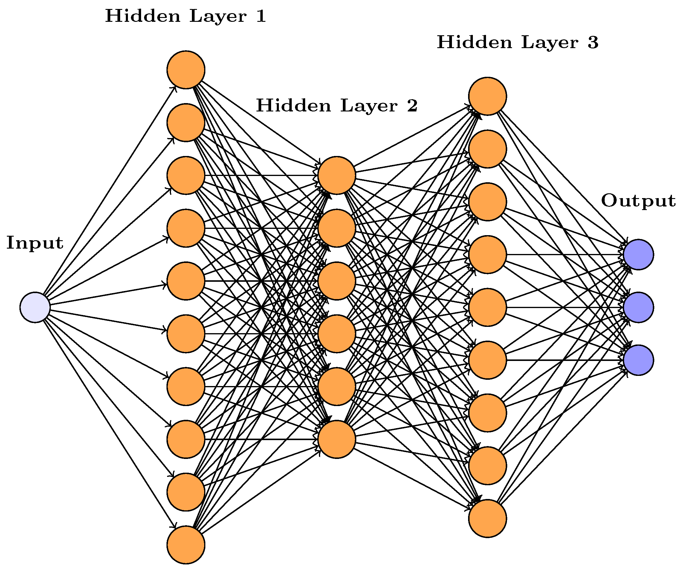
3.1. Feed-Forward Neural Network Architecture

A feed-forward neural network (NN) with three hidden layers as on Figure 1 was constructed to learn the temporal dynamics of the system. The architecture is described as follows:
  • Input layer: accepts a single input feature corresponding to time, denoted as t.
  • Hidden layers: Three fully connected hidden layers, with 10.6 and 9 neurons each and using the hyperbolic tangent (tanh) activation function. To promote stable learning, weights were initialized to small values and biases were set to zero.
  • Output layer: A fully connected layer with three outputs, representing the estimated values of the variables x ( t ) , y ( t ) , and z ( t ) . Each output is connected to a regression layer, which calculates the loss based on the deviation between predicted and actual values.
  Function of the neural network:
  • Time-series prediction: The neural network is trained on datasets ( x , y , z ) to learn and predict their evolution over time. Once trained, it produces predictions for the three variables based solely on time input.
  • Modeling underlying relationships: by learning from data, the NN approximates the hidden relationships between the variables and time, capturing complex and nonlinear behaviors that traditional models might overlook.
  • Preparing for optimization: After prediction, the outputs obtain continuous estimates of the state variables. These are then used to compute numerical derivatives d x d t , d y d t , and d z d t . These derivatives are essential for the next phase of analysis, where model parameters are estimated via optimization using lsqnonlin.
In essence, the neural network plays a crucial role in approximating the dynamics of the system, bridging the gap between observed data and the differential equations required for parameter identification. The neural network architecture with three hidden layers consisting of 10, 6, and 9 neurons respectively was selected based on bootstrap validation performance. Using moving block bootstrap resampling to simulate multiple training and testing scenarios, we compared several candidate architectures. The 10-6-9 configuration consistently achieved the lowest average test error and exhibited minimal performance variance across bootstrap samples, indicating strong generalization capability and robustness to data perturbations. The network’s depth allowed it to model nonlinear interactions among crypto market variables, while its compact structure minimized overfitting.

3.2. Feed-Forward Propagation

A feedforward neural network processes data points through a sequence of operations, as outlined in [29]. Given an input data point t ( m ) , the forward propagation begins by initializing the first layer activation as r 1 [ 0 ] = t ( m ) . To obtain the activations of layer l, denoted r l , from those of the previous layer r l 1 , two main steps are followed.
First, an intermediate vector, c l , is calculated by multiplying the weight matrix W l with r l 1 and then adding the corresponding bias vector b l :
c j l = k = 1 h l 1 W j k l r k l 1 + b j l .
This operation can be compactly written in matrix form as follows:
c l = W l r l 1 + b l .
The second step applies the activation function σ l element-wise to c l , producing the output activations r l :
r l = σ l ( c l ) = σ l W l r l 1 + b l .
Thus, for each input t ( m ) , both the pre-activation values, c l , and the activated outputs, r l , are computed using Equations (6) and (7). To highlight the dependence on the input sample, t ( m ) , we can denote these layer-wise computations as r l ( m ) = σ l ( c l ( m ) ) . In matrix notation, the forward propagation for the entire dataset is summarized as follows:
T = [ t 1 , , t N ] , c l = [ c l ( 1 ) , , c l ( N ) ] , A l = [ r l ( 1 ) , , r l ( N ) ] .
This leads to a recursive formulation for the forward pass:
A 0 = T , c l = W l A l 1 + b l , A l = σ l ( c l ) , for l = 1 , , L .
The final network output, represented as A L , is a function of the input and the learned parameters:
N ( T , W L , b L ) = A L .
Alternatively, we may express the output in component form as follows:
N j ( t ( m ) , W L , b L ) = π j ( A L ) = A j L ( t ( m ) , W , b ) ,
where π j in (11) denotes the extraction of the j-th component from the final output vector A L .

4. Hybrid Neural Network—ODE Framework for Parameter Estimation and Forecasting

This section outlines the methodology developed to estimate parameters in dynamic systems governed by nonlinear ordinary differential equations (ODEs). Our approach utilizes a feedforward neural network in combination with optimization techniques to infer the unknown parameters. To demonstrate its practical utility, we apply the method to a Lotka–Volterra model describing the interactions among three major segments of the cryptocurrency market: Bitcoin, Ethereum, and altcoins. Time-series data for each segment is used, and the results highlight the model’s ability to accurately capture the system’s dynamic behavior.
Accurate parameter estimation in nonlinear dynamic systems is a key challenge across various domains, including financial forecasting. Traditional techniques often rely on simplifications such as linearization or require detailed prior knowledge of the system’s internal structure—assumptions that may not hold in complex financial ecosystems. In this work, we introduce a data-driven approach that leverages the flexibility of neural networks to model intricate dependencies, while employing numerical optimization to estimate the parameters of a nonlinear model. To provide clarity on the implementation, we also present the core steps of the algorithm used in our framework.

4.1. Mathematical Formulation

As we see in Algorithm 1, the neural network is trained to approximate the time evolution of the system by learning the mapping from time to the observed data [30]. After predicting the trajectories, we numerically compute the derivatives and fit them to a generalized Lotka–Volterra (GLV) model using nonlinear least squares optimization. The system of ODEs used to model the interactions among the three components (e.g., BTC, ETH, and ALTs) is given as follows:
d u 1 d t = u 1 p 1 + p 2 u 1 + p 3 u 2 + p 4 u 3 , d u 2 d t = u 2 p 5 + p 6 u 1 + p 7 u 2 + p 8 u 3 , d u 3 d t = u 3 p 9 + p 10 u 1 + p 11 u 2 + p 12 u 3 .
Algorithm 1 Proposed method
1:
Input: Crypto market share data from Excel file, time vector t _ d a t a = [ 0 , 1 , , N 1 ] T
2:
Read and preprocess data [ B T C , E T H , A L T ] into d a t a
3:
Split data into 70% training ( t r a i n _ d a t a , t r a i n _ t i m e ) and 30% testing ( t e s t _ d a t a , t e s t _ t i m e )
4:
Define a Feedforward Neural Network with 3 hidden layers (tanh activation) and linear output
5:
Initialize best weights and minimum validation cost
6:
for each bootstrap iteration b = 1 to 5 do
7:
    Generate moving block bootstrap indices (block length = 10) for training data
8:
    Select resampled training data t r a i n _ d a t a ( b ) , t r a i n _ t i m e ( b )
9:
    Train DNN to predict U ˙ , i.e., the derivatives of market shares ( U ˙ = d U d t ), on t r a i n _ t i m e ( b ) , t r a i n _ d a t a ( b )
10:
    Integrate U ˙ p r e d to obtain U p r e d , i.e., reconstruct predicted market shares from predicted derivatives
11:
    Evaluate on out-of-bag (OOB) data to compute validation cost
12:
    if OOB cost is minimum then
13:
        Store best weights
14:
    end if
15:
end for
16:
Use best weights to compute U p r e d and derivatives d u 1 d t , d u 2 d t , d u 3 d t analytically
17:
Define ODE system: u ˙ i = u i · ( p i 1 + p i 2 u 1 + p i 3 u 2 + p i 4 u 3 ) , i = 1 , 2 , 3
18:
Use nonlinear least squares to estimate parameters p 1 to p 12
19:
Print estimated parameters
20:
Numerical solution fo the Lotka–Volterra equations over the t e s t _ t i m e interval using the Runge–Kutta method
To estimate the parameters p 1 , , p 12 , we define a residual function that quantifies the mismatch between the model’s predicted derivatives and the ones obtained from the neural network output. This residual function is given as follows:
r ( p ) = d u 1 d t u 1 p 1 + p 2 u 1 + p 3 u 2 + p 4 u 3 d u 2 d t u 2 p 5 + p 6 u 1 + p 7 u 2 + p 8 u 3 d u 3 d t u 3 p 9 + p 10 u 1 + p 11 u 2 + p 12 u 3
In Equation (13), the derivatives are obtained from the neural network. Because the network is trained to output u i ( t ) only, each time derivative d u i d t must be computed by analytically differentiating the trained network with respect to t (using the chain rule through every hidden layer). Likewise, when forming r ( p ) for the lsqnonlin call, we should state explicitly that the input “ d u i d t ” is this analytic network derivative, rather than a numerical finite difference. The optimal parameters are obtained by minimizing the sum of squared residuals:
min p r ( p ) 2 2 .
This optimization aligns the dynamics of the GLV model with the data-driven derivatives, effectively capturing the underlying interactions among the system components.

4.2. Numerical Integration via Runge–Kutta

Numerous numerical methods have been developed to solve ordinary differential equations. Among the most widely used for the integration of first- and second-order ODEs are the Runge–Kutta (-Nyström) schemes and linear multistep methods (e.g., see [31,32,33,34,35,36]).
The obtained coefficients are integrated into the Lotka–Volterra system (12), which is solved over the original time span using the classical fourth-order Runge–Kutta method [31]. The simulated trajectories are then compared to the observed data, and RMSE is computed to quantify fit quality.
d y d t = f ( t , y ) , y ( t 0 ) = y 0
The Runge–Kutta method approximates the solution to (15) through an iterative process defined as follows:
y n + 1 = y n + h i = 1 s b i k i , k i = f t n + c i h , y n + h j = 1 i 1 a i j k j , for i = 1 , 2 , , s .
where
  • h represents the time step, s denotes the number of stages in the method, k i are the intermediate stage values, and a i j , b i , c i are coefficients specifying the particular Runge–Kutta scheme.
From the general Runge–Kutta framework (16), various schemes of different algebraic orders can be derived. In this study, we utilize a fourth-order Runge–Kutta method with four stages [31].
Given an initial condition, y ( t 0 ) = y 0 , the solution at the subsequent time step t n + 1 = t n + h is calculated as follows:
k 1 = f t n , y n , k 2 = f t n + c 2 h , y n + a 21 k 1 h , k 3 = f t n + c 3 h , y n + a 31 k 1 + a 32 k 2 h , k 4 = f t n + c 4 h , y n + a 41 k 1 + a 42 k 2 + a 43 k 3 h ,
y n + 1 = y n + h b 1 k 1 + b 2 k 2 + b 3 k 3 + b 4 k 4 .
For the classical RK4 method, the coefficients are as follows:
c 2 = 1 2 , c 3 = 1 2 , c 4 = 1 , a 21 = 1 2 , a 31 = 0 , a 32 = 1 2 , a 41 = 0 , a 42 = 0 , a 43 = 1 , b 1 = 1 6 , b 2 = 1 3 , b 3 = 1 3 , b 4 = 1 6 .
This iterative procedure is applied at each time step, generating an approximate solution to the differential equation described by (15).

4.3. Model Evaluation

The neural network was trained using the Adam optimizer, and epochs with an initial learning rate were selected after experiments with various values. To identify the optimal architecture, three different configurations of hidden layers were evaluated. In addition, multiple activation functions were tested, but the hyperbolic tangent (tanh) proved most effective, delivering the most stable and accurate results.
For performance evaluation, a moving block bootstrap validation approach was employed. This method resamples blocks of the original time series to generate multiple training and testing datasets, preserving temporal dependencies within each block. Unlike traditional cross-validation or walk-forward methods, bootstrap validation is particularly useful when dealing with limited data or non-stationary time series [37]. It allows for robust statistical inference and a more comprehensive understanding of the model’s generalization performance across different subsets of the data. We chose a block length of 10 time steps to span roughly one calendar month of share data, under the assumption that correlations persist over that window. We ran five bootstrap replicates, which we found sufficient to stabilize the out-of-bag (OOB) cost minima in preliminary tests. For each replicate, the OOB indices consist of all training points not selected for any block; the OOB cost is then computed on those held-out points to estimate generalization error. The replicate producing the lowest OOB cost is retained for the final neural-network weights. While we acknowledge that a larger number of bootstrap iterations is ideal for quantifying model uncertainty, the limited size of our dataset (93 observations) imposes practical constraints on both the statistical value and computational feasibility of increasing the bootstrap count. With a small dataset, extensive bootstrapping can lead to high overlap and reduced independence among bootstrap samples, thereby providing diminishing returns in terms of additional information. Prior studies in similar settings [38] have found that even a modest number of bootstrap replications (e.g., 5–10) can still provide a reasonable indication of variability and uncertainty, particularly when computational costs are high and data are limited. By applying this resampling technique, we obtained a realistic and statistically grounded estimate of the network’s prediction accuracy under data variability.
During training, a dynamic plot was used to monitor convergence and track loss reduction in real time. Once training was complete, the model was used to predict the time-dependent variables x(t), y(t), and z(t) across the full time horizon. The performance of the proposed method is highly influenced by both the choice of activation function and the strategy used for initializing weights and biases. The tanh function was chosen over sigmoid and ReLU because it centers outputs around zero, aiding in faster convergence and improving gradient propagation. Unlike sigmoid, tanh offers stronger gradients and mitigates the vanishing gradient issue, while also avoiding the “dead neuron” problem often associated with ReLU. Initial weights were drawn from a distribution of small values to keep the activation functions within their linear regions during early training, which promotes more stable learning dynamics. Similarly, initializing biases with small values prevents early saturation and preserves symmetry breaking across neurons. These combined practices contribute to improved stability, faster convergence, and higher accuracy, making the proposed framework well suited to estimating parameters in complex nonlinear systems such as those modeling cryptocurrency market dynamics.
To address model sensitivity, we performed an extensive grid search varying the number of neurons in each hidden layer from 2 to 5, and from 10 to 15, as well as different learning rates and epochs. The most promising performance was consistently observed when the architecture ranged between 5 to 10 neurons per hidden layer, which we adopted as the focus of our main experiments. Table 1 presents the RMSE results across this comprehensive grid of neural network architectures and hyperparameter settings. The results show that, while some variation in RMSE exists across architectures, the overall pattern remains consistent, with the 10–6–9 architecture providing the lowest mean RMSE. This analysis demonstrates that our findings are robust to reasonable changes in network structure and training configuration. By presenting both the numerical results and our interpretation, we provide evidence that the main conclusions of the study do not depend sensitively on a single neural network architecture or hyperparameter setting.
From Algorithm 2, we see that the DNN searched over all 6 3 = 216 possible three-hidden-layer DNN architectures (from 5 to 10 neurons per layer), for each learning rate and epoch combination.
Algorithm 2 Selection of best neural network architecture
1:
Input: Crypto market share data; Search over hidden layer sizes h 1 , h 2 , h 3 = 5 10 ; Learning rates { 0.00005 , 0.0001 } ; Epochs { 100 , 200 }
2:
for each combination of ( h 1 , h 2 , h 3 ) , learning rate, and epoch count do
3:
    for each bootstrap replicate b = 1 to 5 do
4:
        Train the FFNN on a moving-block bootstrap sample of training data
5:
        Evaluate out-of-bag (OOB) validation cost for this replicate
6:
        Save weights of the replicate with lowest OOB cost
7:
    end for
8:
    Estimate ODE parameters via least-squares using NN output; simulate with RK4; compute RMSE for BTC, ETH, ALTs
9:
    Store architecture configuration and RMSE
10:
end for
11:
Sort all architectures by mean RMSE (RK4 simulation); select the top 10
From Table 1, we select the best architecture based on the mean RMSE. RMSE evaluates the accuracy of predictions by measuring the average error between observed and predicted value, based on a validation procedure:
RMSE = 1 n i = 1 n y i y ^ i 2
Then, we extract the coefficients for all three and solve the system using the fourth-order Runge–Kutta method. Based on the comparison of the mean RMSE, we choose the best one, which we then include in the graphs.

5. Numerical Experiment

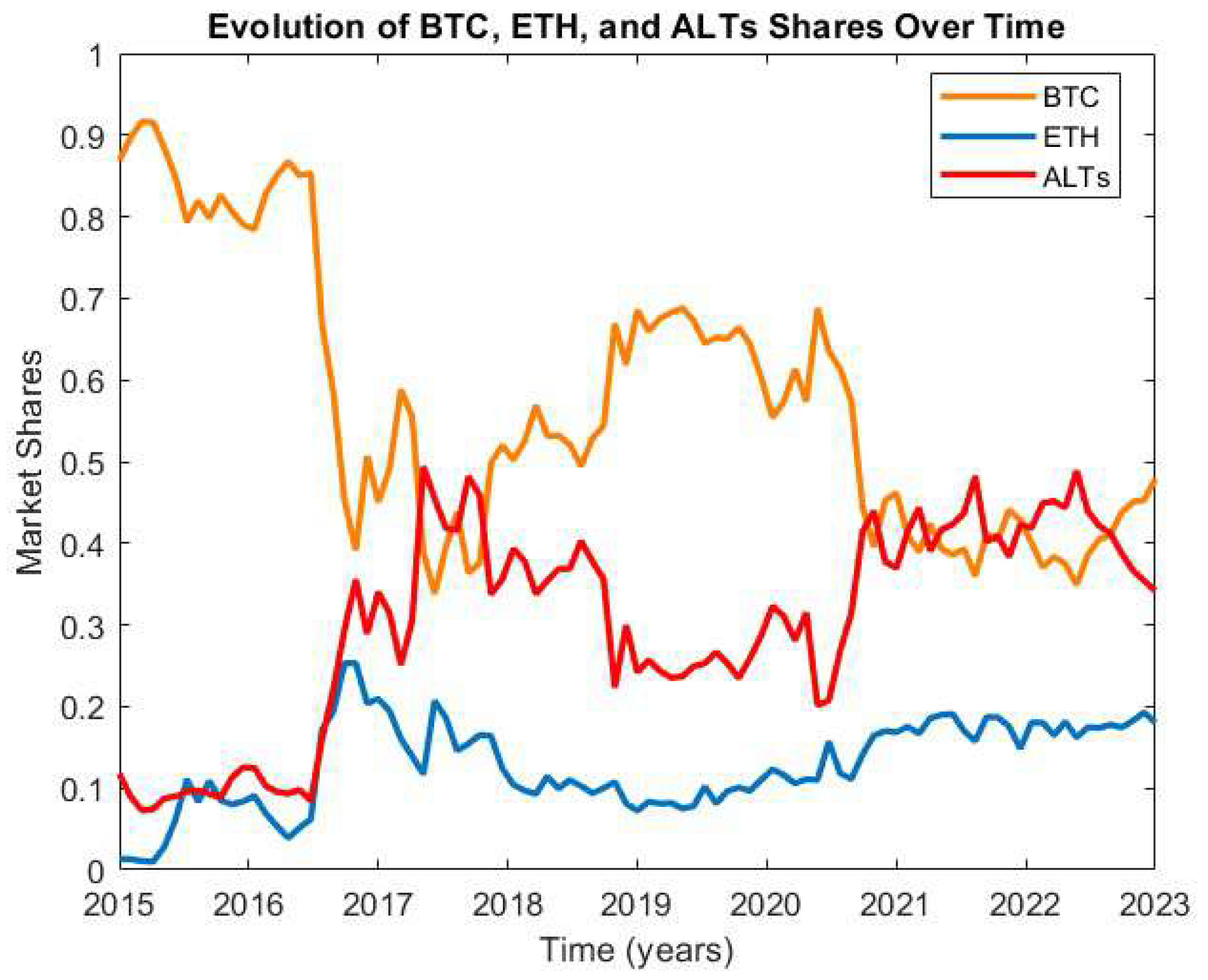
5.1. Case Study Description

This study examines the historical market penetration and future prospects of the three crypto competitors. Monthly market share data for Bitcoin (BTC), Ethereum (ETH), and altcoins (ALTS) were sourced from CoinMarketCap historical snapshots [39], covering August 2015 to May 2023, as shown in Figure 2, a period of 93 months (almost 8 years).
The market share of alternative cryptocurrencies (ALTs) is derived by subtracting the shares of Bitcoin (BTC) and Ethereum (ETH) from 1, ensuring that the total market share across all segments sums to unity.
The initial step in assessing the performance of the proposed framework involves estimating the parameters of the Lotka–Volterra system defined in Equation (2). While traditional approaches typically rely on predefined assumptions derived from the data, this study adopts a data-driven strategy. Specifically, a deep neural network is employed to infer the system parameters by effectively “training” the model based on time-series data of cryptocurrency market shares. This neural network-based estimation replaces heuristic techniques and enables the model to capture the underlying dynamics through optimization and learning from observed behavior. The results of the application of DNN for the case studied provided the following values for the corresponding parameters:
d x d t = x 0.5358 0.4521 x + 0.7681 y 1.3624 z , d y d t = y 1.4664 1.2830 x 1.6997 y 1.7748 z , d z d t = z 0.1941 0.1602 x 0.5119 y 0.1015 z .
The estimated parameters, derived from neural network–assisted system identification, provide a quantitative picture of the mutual influences and self–regulatory mechanisms among Bitcoin (BTC, x), Ethereum (ETH, y), and Altcoins (ALTs, z) in the cryptocurrency market. The associated uncertainty quantification, as reported on Table 2, indicates that while some interactions are well identified, others remain uncertain, and thus, all findings must be interpreted in this context.
Intrinsic growth rates and uncertainty:
  • The intrinsic growth rates— p 1 = 0.5358 for BTC, p 5 = 1.4664 for ETH, and p 9 = 0.1941 for ALTs—suggest that BTC and ETH may experience positive baseline growth in isolation, while ALTs are closer to neutral. The confidence interval for BTC is relatively narrow (low uncertainty), while those for ETH and ALTs are much wider, reflecting high or medium uncertainty and indicating that considerable variability is possible.
Intraspecies (self-interaction) terms and uncertainty:
  • The self-interaction parameters p 2 = 0.4521 (BTC, low uncertainty), p 7 = 1.6997 (ETH, high uncertainty), and p 12 = 0.1015 (ALTs, high uncertainty) are negative, consistent with self-limitation effects. However, only the BTC self-limitation is statistically well identified; ETH and ALT self-regulation remain uncertain due to wide confidence intervals and large standard errors.
Interspecies interactions and uncertainty:
  • Parameters reflecting competition or inhibition between asset classes—such as p 3 = 0.7681 , p 4 = 1.3624 , p 6 = 1.2830 , p 8 = 1.7748 , p 10 = 0.1602 , and p 11 = 0.5119 —vary in both sign and certainty. BTC-related cross-interactions ( p 3 and p 4 ) are estimated with medium uncertainty, while most others, particularly those involving ETH and ALTs, have high uncertainty, meaning the direction and strength of these effects cannot be robustly established from the current data.
Summary and implications:
Overall, the model reveals that some self-regulation and mutual inhibition mechanisms—especially for BTC—are reliably identified, while the interactions involving ETH and ALTs remain uncertain, as shown by their wide confidence intervals and high standard errors. This uncertainty is likely due to intrinsic market volatility, data limitations, and the complexity of the cryptocurrency ecosystem. The parameter values should, therefore, be regarded as indicative, rather than definitive.
Future research leveraging more extensive data, models allowing for time-variation in parameters, or introducing regularization techniques could help reduce uncertainty and yield more robust and interpretable estimates. Stability analyses and further predictions should explicitly account for these uncertainty levels.

5.2. System Stability Testing

To investigate the local dynamics of the crypto market share model, we first estimate the parameters p i and p i j from observed market data using a neural network combined with optimization techniques. These parameters define the nonlinear Lotka–Volterra system (12), where u i represents the market shares of BTC, ETH, and ALTs, respectively.
It is important to note that these parameter estimates exhibit a degree of uncertainty, as quantified using bootstrap confidence intervals. Therefore, the following equilibrium and stability analyses [40] should be interpreted as conditional on the current parameter estimates and their variability.
By setting the time derivatives to zero,
d u i d t = 0 ,
we solve the resulting algebraic system and find a candidate equilibrium of approximately 41 % for BTC, 20 % for ETH, and 39 % for ALTs:
u * = ( 0.4150 , 0.1953 , 0.3897 ) .
This represents the predicted steady-state market shares under the estimated parameters.
To understand the local behavior near this equilibrium, we linearize the nonlinear system (12) around u * . With deviations from the equilibrium denoted as
U = u 1 u 1 * , V = u 2 u 2 * , W = u 3 u 3 * ,
the linearized dynamics satisfy
d d t U V W = J ( u * ) U V W ,
where J ( u * ) is the Jacobian matrix of partial derivatives evaluated at the equilibrium.
The general solution near equilibrium is
U V W = c 1 v 1 e λ 1 t + c 2 v 2 e λ 2 t + c 3 v 3 e λ 3 t ,
where λ i and v i are the real eigenvalues and eigenvectors of J ( u * ) , and the coefficients c i are obtained by projecting the initial deviation onto the eigenvector basis:
c 1 = 0.1583 , c 2 = 0.1082 , c 3 = 0.5636 .
Analyzing the eigenvalues of J ( u * ) , we find
λ 1 = 0.4850 , λ 2 = 0.2072 , λ 3 = 0.0013 ,
all strictly negative, suggesting that u * is locally asymptotically stable under the current parameter estimates. The absence of imaginary parts indicates monotonic convergence without oscillations.
However, given the presence of uncertainty in some parameters, the precise location and stability properties of u * may vary in practice. This analysis assumes time-invariant parameters and neglects exogenous shocks, which are important factors in real cryptocurrency markets.
The phase portrait shown in Figure 3 displays trajectories initiated from diverse initial conditions. All trajectories converge smoothly to the equilibrium u * , supporting the model’s predictive validity within the assumptions and current parameter estimates.
Overall, this approach—combining parameter estimation with Lotka–Volterra equilibrium and stability analysis—provides a useful framework to characterize the system’s local dynamics, though further work is needed to incorporate parameter uncertainty, time variability, and external influences for more robust market predictions.

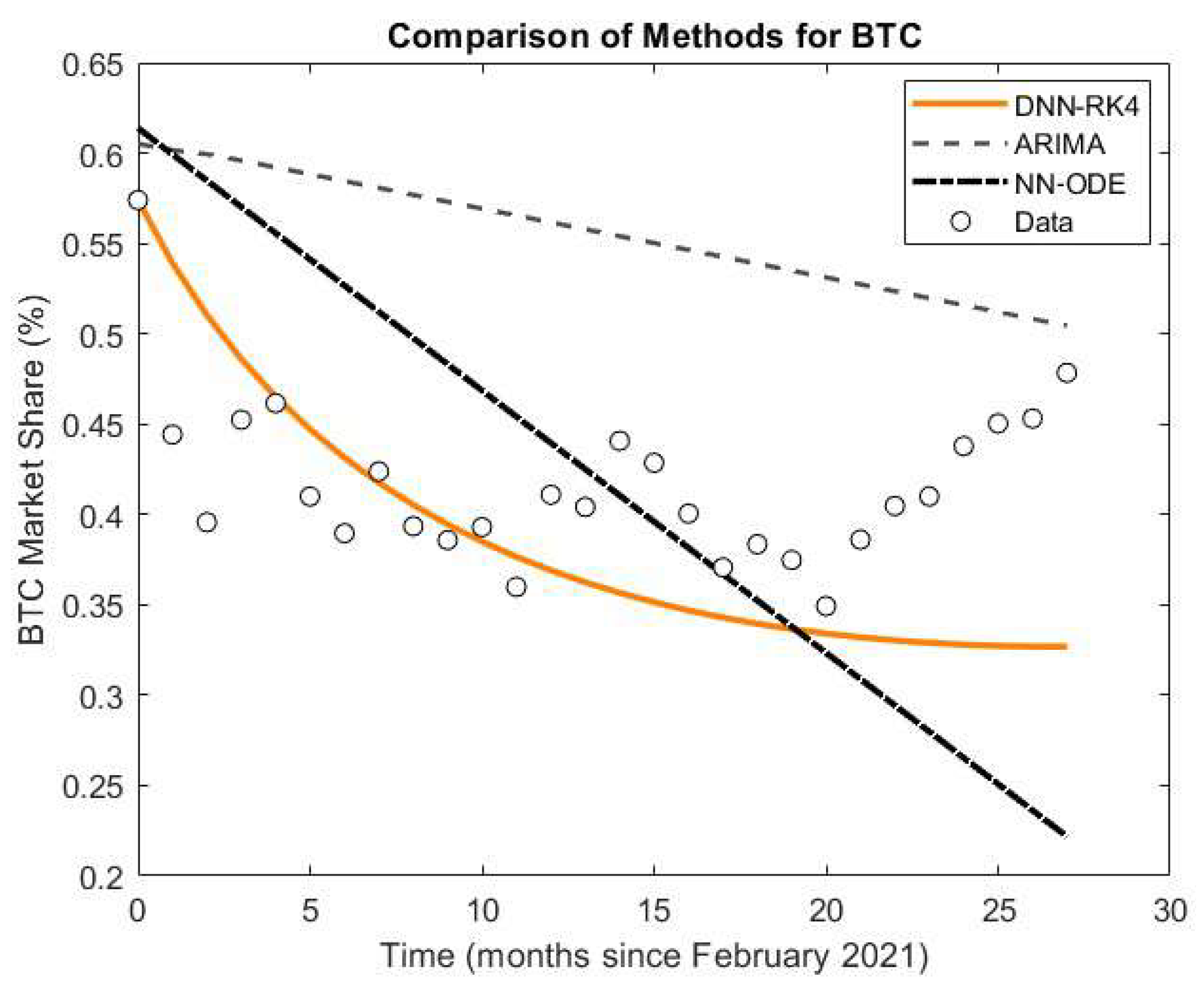
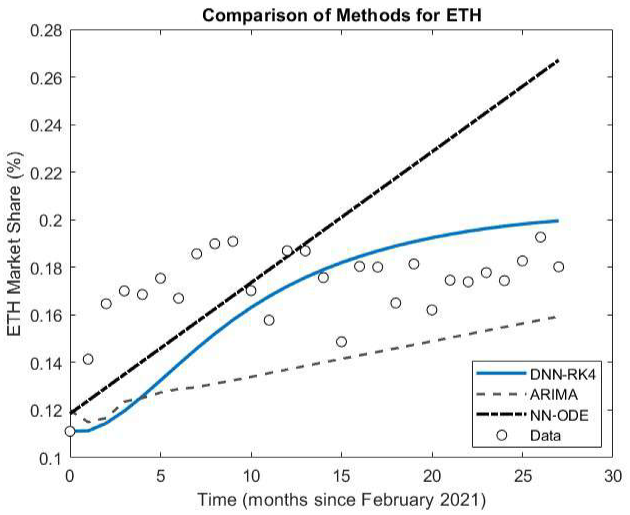
5.3. Case Study Results

In this section, we compare the effectiveness of our hybrid DNN-RK4 method against a range of ARIMA models and a neural ODE (NN-ODE) approach for predicting the market shares of BTC, ETH, and ALTs. The DNN-RK4 approach demonstrates the closest alignment to the real-world market share data, consistently producing the lowest prediction errors across the tested period.
The ARIMA (autoregressive integrated moving average) model is a widely used statistical method for analyzing and forecasting time-series data. It combines three components: the autoregressive (AR) part models the relationship between current and past values; the integrated (I) part handles non-stationarity by differencing the data; and the moving average (MA) part captures dependencies between residual errors. By adjusting its parameters (p, d, and q), ARIMA can effectively model and forecast trends and patterns in sequential financial data, including cryptocurrency prices. In the ARIMA ( p , d , q ) model, p denotes the order of the autoregressive component (i.e., the number of lagged values of the series included), d represents the degree of differencing applied to make the series stationary (i.e., the number of times the series is replaced by the difference between consecutive observations), and q specifies the order of the moving-average component (i.e., the number of lagged forecast errors incorporated). Together, these three parameters allow ARIMA models to capture both short-term autocorrelation (through p and q) and nonstationarity (through d) in time series data.
The neural ODE (NN-ODE) model is a deep learning approach for modeling time series dynamics by parameterizing the system of differential equations with neural networks. Instead of specifying fixed functional forms, NN-ODE learns the underlying evolution rules directly from the data. This allows the model to flexibly capture nonlinear and complex relationships in sequential data. The network is trained to minimize the difference between observed and predicted trajectories, using methods like Runge–Kutta for integrating the neural dynamics over time. As a result, NN-ODE offers a data-driven way to forecast system evolution, especially useful when the true governing equations are unknown or highly nonlinear.
The various ARIMA configurations [41], while capable of capturing some of the underlying temporal patterns, generally yield higher root mean squared error (RMSE) values compared to the DNN-RK4 method. To facilitate an objective assessment, all models, including NN-ODE, are evaluated using the RMSE metric, and results are summarized both in graphical form and in a results table.
This analysis provides strong evidence that the DNN-RK4 method offers superior predictive power for modeling the evolution of cryptocurrency market shares when compared to traditional ARIMA time series approaches and the neural ODE method.
To evaluate the forecasting accuracy of the proposed DNN-RK4 approach, grounded in a nonlinear dynamical system framework, we compared its performance with that of classical time series models, specifically ARIMA, as well as the NN-ODE model. We evaluated multiple ARIMA ( p , d , q ) configurations, including ( 2 , 1 , 2 ) , ( 2 , 1 , 1 ) , and ( 1 , 0 , 1 ) . For each candidate model, we fitted the parameters on the training set and computed the RMSE on the validation set. The ARIMA ( 2 , 1 , 2 ) configuration produced the lowest RMSE, and was therefore chosen for comparison against our proposed method and NN-ODE. To optimize the NN-ODE model, we conducted an extensive grid search, varying the number of neurons in each of the three hidden layers from 3 to 10, with learning rates of 0.0001 and 0.001 and training epochs of 100 and 200. The mean RMSE (MRMSE) across all assets was used as our primary evaluation metric to identify the best configuration. This systematic process led to the selection of a 5–4–10 architecture with a learning rate of 0.001 and 200 training epochs, which consistently provided the lowest MRMSE and was adopted for our main experiments. The comparison focuses on the three main components of the market: Bitcoin (BTC), Ethereum (ETH), and alternative cryptocurrencies (ALTs).
The DNN-RK4 model, driven by parameters estimated through a neural network, exhibited superior predictive performance across all market segments. For BTC, the DNN-RK4 model achieved an RMSE of 0.06865, significantly outperforming the ARIMA model’s RMSE of 0.14742 and the NN-ODE’s RMSE of 0.11757, as we notice in Figure 4. In the case of ETH, we see on Figure 5 that the differential was similarly notable—0.02682 (DNN-RK4) compared to 0.03665 (ARIMA) and 0.04507 (NN-ODE). For the ALT category, the DNN-RK4 model again showed improved accuracy, reducing the error from 0.11890 (ARIMA) and 0.11305 (NN-ODE) to 0.05581 as shown in Figure 6. These results highlight the advantage of using a model based on competitive dynamics to capture nonlinear relationships inherent to the cryptocurrency ecosystem, where investor behavior, technological updates, and market sentiment evolve rapidly.
The cryptocurrency market is characterized by high volatility, interdependence between major assets, and the continuous entry of new tokens. These features make traditional linear models less effective in capturing complex feedback mechanisms and competitive interactions. The DNN-RK4 method, supported by neural network-driven parameter learning, demonstrates strong adaptability in forecasting such nonlinear systems. It is particularly useful in capturing turning points and saturation effects, which are common in speculative and innovation-driven markets like crypto.
Further supporting these observations, Table 3 now compares both RMSE and MAE values across multiple modeling strategies. To underscore the practical benefits of our DNN–RK4 hybrid model, we present a concise overview of its forecasting performance relative to ARIMA and NN-ODE. The following summary distills the key RMSE improvements for each asset class.
  • BTC: DNN–RK4 halves the error of ARIMA (0.0687 vs. 0.1474 RMSE).
  • ETH: DNN–RK4 outperforms by approx. 27% (0.0268 vs. 0.0367 RMSE).
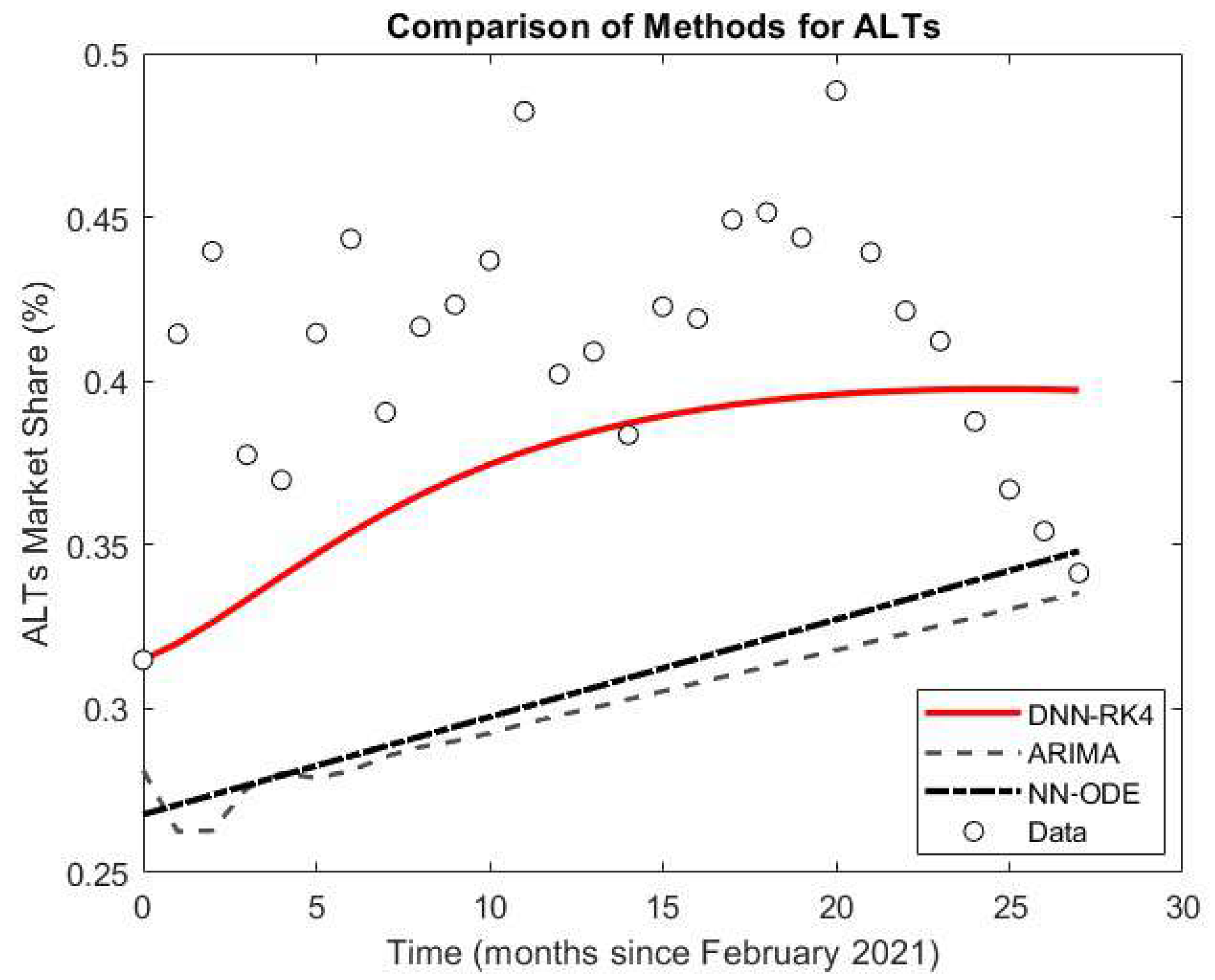
  • ALTs: DNN–RK4 reduces error by approx. 53% (0.0558 vs. 0.1189 RMSE).
  • Aggregate: Mean RMSE drops from 0.101 (ARIMA) and 0.092 (NN–ODE) to 0.050 (DNN–RK4).
While RMSE has been our main evaluation criterion throughout the study, we also report MAE to provide a more robust and comprehensive assessment of forecasting accuracy, as MAE is less sensitive to large outliers.
MAE = 1 n i = 1 n | y i y ^ i |
The DNN-RK4 model, in particular, demonstrated excellent performance, with RMSE values of 0.06865, 0.02682, and 0.05581 and corresponding MAE values of 0.05432, 0.02259, and 0.04735 for BTC, ETH, and ALTs, respectively. Notably, the mean MAE for DNN-RK4 (0.04142) was substantially lower than for ARIMA (0.09420) and NN-ODE (0.07965). This dual-metric analysis further confirms that DNN-RK4 consistently yields the most accurate predictions for cryptocurrency market shares among the methods compared.

6. Discussion

In recent years, the intersection of machine learning and dynamical systems has opened new directions for financial and economic modeling, especially in challenging environments like cryptocurrencies. Our work builds on these methodological developments, drawing inspiration from state-of-the-art deep learning architectures such as LSTM networks [42] and more recent advances using attention mechanisms and transformer models [43], which have demonstrated impressive forecasting accuracy in financial applications, including the crypto sector [44]. In addition to modeling price dynamics, modern approaches increasingly incorporate macroeconomic variables—for example, central bank policy rates—to explain asset fluctuations and regime shifts [45]. By grounding our approach in this broader context, we aim to bridge endogenous competition models with the latest advances in machine learning, highlighting the relevance and potential extensions of our framework to wider financial systems.
To further improve the robustness and accuracy of cryptocurrency market modeling, future research will investigate a range of advanced machine learning and hybrid approaches tailored to the unique challenges of crypto dynamics. One promising direction involves temporal convolutional networks (TCNs) [46], which can outperform recurrent models in sequence modeling tasks while offering parallel processing advantages and stable gradients over long sequences—a critical factor—in training stability when analyzing extensive crypto market histories.
In addition, the use of graph neural networks (GNNs) will be explored to represent the complex interdependencies between different cryptocurrencies [47]. Crypto assets often exhibit co-movements, influenced by trading volumes, blockchain correlations, or investor sentiment. Modeling these relationships as a graph enables more informed parameter estimation and can uncover hidden structures in the market.
Another area of potential is neural ODEs [48], which integrate the strengths of neural networks with differential equations. This approach is particularly suitable for learning continuous-time representations, offering a natural fit for systems like Lotka–Volterra that evolve over time. Neural ODEs can adaptively model temporal changes in market competition and volatility with fewer parameters and better interpretability [49].
The integration of sentiment analysis from social media and blockchain news will also be considered. Since investor behavior in crypto is highly reactive to news, incorporating textual data through models like BERT or domain-specific transformer variants (e.g., FinBERT) could improve forecasting accuracy by providing context-aware inputs to dynamic models [50]. Finally, online learning techniques will be examined for their ability to continuously update model parameters as new data arrives. This is critical for maintaining prediction accuracy in a market characterized by rapid innovation, regulatory shifts, and speculative bubbles. Something important to note here is that, because our Lotka–Volterra model assumes constant coefficients, it cannot capture one-time shocks such as Bitcoin’s May 2020 halving or regulatory crackdowns in 2021. As a result, the estimated parameters may partially reflect these exogenous events, rather than pure “peer competition.” Also, a limitation of our current study is the exclusion of external market covariates such as absolute price, trading volume, and macroeconomic factors. While our results focus on modeling relative competition within a closed system, future research should include control experiments that explicitly incorporate such exogenous variables to quantify their impact on market share evolution. Future work will incorporate time-varying coefficients, exogenous covariates, and the previously discussed methodologies to address this limitation, aiming to develop a more comprehensive, adaptive, and robust framework for modeling and forecasting market share evolution in the cryptocurrency domain.

7. Conclusions

The proposed framework demonstrates that integrating deep neural networks with Lotka–Volterra competitive dynamics provides a robust, data-driven means of capturing and forecasting the evolving structure of cryptocurrency market shares. By estimating interaction coefficients directly from observed BTC, ETH, and ALT time series and then simulating their joint evolution via a fourth-order Runge–Kutta scheme, the model not only outperforms traditional ARIMA benchmarks but also achieves lower prediction errors compared to a standard NN-ODE model. Our hybrid DNN-RK4 approach achieves a mean RMSE of 0.05001 and a mean MAE of 0.04099, significantly outperforming ARIMA (mean RMSE 0.10099, mean MAE 0.09420) and NN-ODE (mean RMSE 0.09190, mean MAE 0.07965) across all assets. This confirms the superior accuracy and practical effectiveness of our method for cryptocurrency market forecasting, indicating its practical potential for decision-making in portfolio management and market trend analysis. Furthermore, the Lotka–Volterra–NN hybrid approach yields interpretable insights into mutual competitive pressures (e.g., the asymmetric influence of BTC on ALTs and ETH on BTC). Moreover, a local stability analysis indicates that the estimated equilibrium is locally asymptotically stable for the best-fit parameters, explaining why any transient deviations decay in the absence of exogenous shocks. However, since some parameters exhibit medium to high uncertainty, this stability conclusion is conditional on the estimated values; further analysis is warranted to assess how parameter uncertainty might affect the robustness of equilibrium stability. These findings both validate the Lotka–Volterra–NN hybrid approach in a highly nonlinear, volatile domain and furnish a principled basis for strategic decision-making. The key limitations of this study include the exclusion of macroeconomic and exogenous variables and the assumption of constant interaction parameters. Looking ahead, extending the model to accommodate time-varying coefficients, exogenous covariates, or graph-based interactions among a broader set of tokens could further enhance its adaptability and predictive power, ensuring that it remains responsive to the rapid innovation and intermittent shocks characteristic of global crypto markets.

Supplementary Materials

The following supporting information can be downloaded at https://www.mdpi.com/article/10.3390/fi17080327/s1, Spreadsheets S1: Crypto Data.

Author Contributions

D.K., D.P., and K.G. conceived of the idea, designed and performed the experiments, analyzed the results, drafted the initial manuscript, and revised the final manuscript. All authors have read and agreed to the published version of the manuscript.

Funding

This research was supported by Grant (81845) from the Research Committee of the University of Patras via “C. CARATHEODORI” program.

Data Availability Statement

The raw data used in this study are publicly available online at https://coinmarketcap.com/historical/. The specific dataset used for analysis is also provided in the Supplementary Materials (accessed on 8 March 2025).

Conflicts of Interest

The authors declare no conflicts of interest.

References

  1. White, G.R. Future applications of blockchain in business and management: A Delphi study. Strateg. Change 2017, 26, 439–451. [Google Scholar] [CrossRef]
  2. Bitcoin.org. Available online: https://bitcoin.org/bitcoin.pdf (accessed on 2 April 2025).
  3. Tradingview.com. Available online: https://www.tradingview.com/symbols/BTC/ (accessed on 5 April 2025).
  4. Taleb, N. Prospective applications of blockchain and bitcoin cryptocurrency technology. TEM J. 2019, 8, 48–55. [Google Scholar] [CrossRef]
  5. Navamani, T.M. A Review on Cryptocurrencies Security. J. Appl. Secur. Res. 2021, 18, 49–69. [Google Scholar] [CrossRef]
  6. Nandy, T.; Verma, U.; Srivastava, P.; Rongara, D.; Gupta, A.; Sharma, B. The Evaluation of Cryptocurrency: Overview, Opportunities, and Future Directions. In Proceedings of the 2023 7th International Conference on Intelligent Computing and Control Systems (ICICCS), Madurai, India, 17–19 May 2023; pp. 1421–1426. [Google Scholar]
  7. Tradingview.com. Available online: https://www.tradingview.com/symbols/ETH/ (accessed on 8 April 2025).
  8. Forbes.com. Available online: https://www.forbes.com/sites/lawrencewintermeyer/2021/08/12/institutional-money-is-pouring-into-the-crypto-market-and-its-only-going-to-grow/?sh=1a5424261459 (accessed on 8 April 2025).
  9. Taleb, N.N. Bitcoin, currencies, and fragility. Quant. Financ. 2021, 21, 1249–1255. [Google Scholar] [CrossRef]
  10. Visual Capitalist. Available online: https://www.visualcapitalist.com/crypto-ownership-growth-by-region/ (accessed on 12 April 2025).
  11. Javarone, M.A.; Wright, C.S. From bitcoin to bitcoin cash: A network analysis. In Proceedings of the 1st Workshop on Cryptocurrencies and Blockchains for Distributed Systems, Munich, Germany, 15 June 2018; pp. 77–81. [Google Scholar]
  12. Donet, J.A.D.; Pérez-Sola, C.; Herrera-Joancomartí, J. The bitcoin p2p network. In Proceedings of the International Conference on Financial Cryptography and Data Security, Christ Church, Barbados, 3–7 March 2014; pp. 87–102. [Google Scholar]
  13. Kjærl, F.; Khazal, A.; Krogstad, E.A.; Nordstrøm, F.B.; Oust, A. An analysis of bitcoin’s price dynamics. J. Risk Financ. Manag. 2018, 11, 63. [Google Scholar] [CrossRef]
  14. Velankar, S.; Valecha, S.; Maji, S. Bitcoin price prediction using machine learning. In Proceedings of the 2018 20th International Conference on Advanced Communication Technology (ICACT), Chuncheon, Republic of Korea, 11–14 February 2018; pp. 144–147. [Google Scholar]
  15. ElBahrawy, A.; Alessandretti, L.; Kandler, A.; Pastor-Satorras, R.; Baronchelli, A. Evolutionary dynamics of the cryptocurrency market. R. Soc. Open Sci. 2017, 4, 170623. [Google Scholar] [CrossRef]
  16. Wu, K.; Wheatley, S.; Sornette, D. Classification of cryptocurrency coins and tokens by the dynamics of their market capitalizations. Soc. Open Sci. 2018, 5, 180381. [Google Scholar] [CrossRef]
  17. Murray, J.D. Mathematical Biology; Springer: New York, NY, USA, 1993. [Google Scholar]
  18. Wijeratnea, A.W.; Yi, F.; Wei, J. Biffurcation analysis in the diffu- sive Lotka-Voltera system: An application to market economy. Chaos Solitons Fractals 2009, 40, 902–911. [Google Scholar] [CrossRef]
  19. Neal, D. Introduction to Population Biology; Cambridge University Press: New York, NY, USA, 2004. [Google Scholar]
  20. Boyce, W.E.; DiPrima, R.C. Elementary Differential Equations and Boundary Value Problems, 8th ed.; Wiley: Hoboken, NJ, USA, 2004. [Google Scholar]
  21. Fisher, J.C.; Pry, R.H. A simple substitution model of technological change. Technol. Forecast. Soc. Change 1971, 3, 75–88. [Google Scholar] [CrossRef]
  22. Rai, L.P. Appropriate models for technology substitution. J. Sci. Ind. Res. 1999, 58, 14–18. [Google Scholar]
  23. Begon, M.; Townsend, C.; Harper, J. Ecology: From Individuals to Ecosystems, 4th ed.; Blackwell: Oxford, UK, 2006. [Google Scholar]
  24. Fay, T.H.; Greeff, J.C. A three species competition model as a decision support tool. Ecol. Modell 2008, 211, 142–152. [Google Scholar] [CrossRef]
  25. Leach, P.G.L.; Miritzis, J. Analytic behaviour of competition among three species. J. Nonlinear Math. Phys. 2006, 13, 535–548. [Google Scholar] [CrossRef]
  26. Olivença, D.V.; Davis, J.D.; Voit, E.O. Inference of dynamic interaction networks: A comparison between Lotka-Volterra and multivariate autoregressive models. Front. Bioinform. 2022, 2, 1021838. [Google Scholar] [CrossRef] [PubMed]
  27. Kastoris, D.; Giotopoulos, K.; Papadopoulos, D. Neural Network-Based Parameter Estimation in Dynamical Systems. Information 2024, 15, 809. [Google Scholar] [CrossRef]
  28. Michalakelis, C.; Sphicopoulos, T.S.; Varoutas, D. Modelling competition in the telecommunications market based on the concepts of population biology. Trans. Syst. Man Cybern. Part C Appl. Rev. 2011, 41, 200–210. [Google Scholar] [CrossRef]
  29. Bebis, G.; Georgiopoulos, M. Feed-forward neural networks. IEEE Potentials 1994, 13, 27–31. [Google Scholar] [CrossRef]
  30. Huang, L.; Qin, J.; Zhou, Y.; Zhu, F.; Liu, L.; Shao, L. Normalization Techniques in Training DNNs: Methodology, Analysis and Application. IEEE Trans. Pattern Anal. Mach. Intell. 2023, 45, 10173–10196. [Google Scholar] [CrossRef]
  31. Butcher, J.C. Numerical Methods for Ordinary Differential Equations; John Wiley & Sons: Hoboken, NJ, USA, 2016; Volume 3, pp. 143–331. [Google Scholar]
  32. Delin, T.; Zheng, C. On A General Formula of Fourth Order Runge-Kutta Method. J. Math. Sci. Math. Educ. 2012, 7, 1–10. [Google Scholar]
  33. Dormand, J.R.; El-Mikkawy, M.E.A.; Prince, P.J. Families of Runge-Kutta-Nyström formulae. IMA J. Numer. 1987, 7, 235–250. [Google Scholar] [CrossRef]
  34. Papadopoulos, D.F.; Simos, T.E. The use of phase lag and amplification error derivatives for the construction of a modified Runge-Kutta-Nyström method. Abstr. Appl. Anal. 2013, 2013, 910624. [Google Scholar] [CrossRef]
  35. Papadopoulos, D.F.; Anastassi, Z.A.; Simos, D.F. The use of phase-lag and amplification error derivatives in the numerical integration of ODEs with oscillating solutions. AIP Conf. Proc. 2009, 1168, 547–549. [Google Scholar]
  36. Papadopoulos, D.F. A Parametric Six-Step Method for Second-Order IVPs with Oscillating Solutions. Mathematics 2024, 12, 3824. [Google Scholar] [CrossRef]
  37. Steyerberg, E.W.; Harrell, F.E., Jr.; Borsboom, G.J.; Eijkemans, M.J.C.; Vergouwe, Y.; Habbema, J.D.F. Internal validation of predictive models: Efficiency of some procedures for logistic regression analysis. J. Clin. Epidemiol. 2001, 54, 774–781. [Google Scholar] [CrossRef]
  38. Efron, B.; Tibshirani, R.J. An Introduction to the Bootstrap, 1st ed.; Chapman and Hall/CRC Press: Boca Raton, FL, USA, 1994. [Google Scholar]
  39. Coinmarketcap.com. Available online: https://coinmarketcap.com/historical/ (accessed on 16 April 2025).
  40. Schulz, A.W. Equilibrium modeling in economics: A design-based defense. J. Econ. Methodol. 2024, 31, 36–53. [Google Scholar] [CrossRef]
  41. Kontopoulou, V.I.; Panagopoulos, A.D.; Kakkos, I.; Matsopoulos, G.K. A Review of ARIMA vs. Machine Learning Approaches for Time Series Forecasting in Data Driven Networks. Future Internet 2023, 15, 255. [Google Scholar] [CrossRef]
  42. Hochreiter, S.; Schmidhuber, J. Long short-term memory. Neural Comput. 1997, 9, 1735–1780. [Google Scholar] [CrossRef]
  43. Vaswani, A.; Shazeer, N.; Parmar, N.; Uszkoreit, J.; Jones, L.; Gomez, A.N.; Kaiser, Ł.; Polosukhin, I. Attention is all you need. In Proceedings of the Advances in Neural Information Processing Systems 30: Annual Conference on Neural Information Processing Systems 2017, Long Beach, CA, USA, 4–9 December 2017; Volume 30. [Google Scholar]
  44. Kim, S.; Shin, D. Transformer-based cryptocurrency price prediction using social media sentiment. IEEE Access 2021, 9, 140697–140709. [Google Scholar]
  45. Choi, I.; Kim, W.C. A temporal information transfer network approach considering federal funds rate for an interpretable asset fluctuation prediction framework. Int. Rev. Econ. Financ. 2024, 96, 103562. [Google Scholar] [CrossRef]
  46. Liu, Y.; Huang, X.; Xiong, L.; Chang, R.; Wang, W.; Chen, L. Stock price prediction with attentive temporal convolution-based generative adversarial network. Array 2025, 25, 100374. [Google Scholar] [CrossRef]
  47. Zhao, Z.; Wang, J.; Wei, J. Graph-Neural-Network-Based Transaction Link Prediction Method for Public Blockchain in Heterogeneous Information Networks. Blockchain Res. Appl. 2025, 6, 100265. [Google Scholar] [CrossRef]
  48. Chen, R.T.Q.; Rubanova, Y.; Bettencourt, J.; Duvenaud, D. Neural Ordinary Differential Equations. Adv. Neural Inf. Process. Syst. 2018, 31, 3–4. [Google Scholar]
  49. Coelho, C.; da Costa, M.F.P.; Ferrás, L.L. XNODE: A XAI Suite to Understand Neural Ordinary Differential Equations. AI 2025, 6, 105. [Google Scholar] [CrossRef]
  50. Gurgul, V.; Lessmann, S.; Härdle, W.K. Deep learning and NLP in cryptocurrency forecasting: Integrating financial, blockchain, and social media data. Int. J. Forecast. 2024, 2, 4. [Google Scholar] [CrossRef]
Figure 1. An example of a deep neural network with one input neuron, three output neurons, and three hidden layers, with 10.6 and 9 neurons.
Futureinternet 17 00327 g001
Figure 2. Evolution of cryptocurrency market from August 2015 to May 2023.
Futureinternet 17 00327 g002
Figure 3. Trajectories from various initial market shares converging to the unique stable equilibrium u * (Blue Star Point).
Futureinternet 17 00327 g003
Figure 4. Actual vs. predicted Bitcoin market-share trajectories (February 2021–May 2023).
Futureinternet 17 00327 g004
Figure 5. Actual vs. predicted Ethereum market-share trajectories (February 2021–May 2023).
Futureinternet 17 00327 g005
Figure 6. Actual vs. predicted Altcoins market-share trajectories (February 2021–May 2023).
Futureinternet 17 00327 g006
Table 1. Per-asset RMSEs (BTC, ETH, and ALTs) and mean RMSE (MRMSE) for various NN architectures and hyperparameters.
h 1 h 2 h 3 BTCETHALTsMRMSELREpochs
10690.0563550.0974970.0965560.0834690.0001200
10690.0632680.0923360.0977580.0844540.0001100
810100.0687670.0976750.1013600.0892670.0001200
7760.0626120.1009600.1024800.0886840.0001200
710100.0714300.0964620.1028600.0902510.0001200
65100.0634370.1018700.1029400.0894160.0001200
91050.0710150.0990510.1031000.0910550.00005200
99100.0686000.0997300.1045400.0909570.0001200
108100.0584090.1140400.1051500.0925330.0001200
91050.0723990.1007900.1052700.0928200.0001100
Table 2. Parameter estimates with uncertainty quantification (using standard error and 95% confidence interval).
ParameterEstimateStd (Uncertainty)95% CI RangeUncertainty Level
p 1 0.53580.0995[0.3409, 0.7308]Low
p 2 −0.45210.0826[−0.6139, −0.2903]Low
p 3 0.76810.1440[0.4859, 1.0502]Medium
p 4 −1.36240.2519[−1.8562, −0.8687]Medium
p 5 1.46642.1373[−2.7227, 5.6554]High
p 6 −1.28301.7878[−4.7871, 2.2210]High
p 7 −1.69972.7787[−7.1458, 3.7465]High
p 8 −1.77485.2371[−12.0395, 8.4899]High
p 9 0.19410.4939[−0.7739, 1.1622]Medium
p 10 −0.16020.4119[−0.9675, 0.6471]Medium
p 11 −0.51190.6752[−1.8352, 0.8115]High
p 12 −0.10151.2280[−2.5085, 2.3054]High
Table 3. Root mean squared error (RMSE) and mean absolute error (MAE) values for different methods and components: BTC, ETH, and ALTs.
MethodBTC (RMSE)ETH (RMSE)ALTs (RMSE)BTC (MAE)ETH (MAE)ALTs (MAE)
DNN-RK40.068650.026820.055810.054320.022590.04735
ARIMA (2,1,2)0.147420.036650.118900.139060.033700.10986
NN-ODE0.117570.045070.113050.097010.038060.10388
Disclaimer/Publisher’s Note: The statements, opinions and data contained in all publications are solely those of the individual author(s) and contributor(s) and not of MDPI and/or the editor(s). MDPI and/or the editor(s) disclaim responsibility for any injury to people or property resulting from any ideas, methods, instructions or products referred to in the content.

