Abstract
Efforts to increase wood mobilization have highlighted the need to appraise drivers of short-run timber supply. The current study aims to shed further light on harvesting decisions of private forest owners, by investigating optimal harvesting under uncertainty, when timber revenues are invested on financial markets and uncertainty is mitigated by news releases. By distinguishing between aggregate economic risk and sector specific risks, the model studies in great detail optimal harvesting-investment decisions, with particular emphasis on the non-trivial transmission of risk on optimal harvesting, and on the way private forest owners react to news and information. The analysis of the role played by information in harvesting decisions is a novelty in forest economic theory. The presented model is highly relevant from a policy—information is a commonly used forest policy instrument—as well as a practical perspective, since the mechanism of risk transmission is at the basis of timber pricing.
Keywords:
wood mobilization; timber supply; decision; uncertainty; risk; information; portfolio; financial market 1. Introduction
1.1. Background
Forest ownership structure is known to have implications for forest management and the production of timber and other forest products and services [1]. In the forest-rich regions of Central-East and Northern Europe, private forest ownership is increasing at the expense of public ownership (Ibid.), a process often linked to the fragmentation of forest land and ensuing difficulties in mobilizing woody biomass [2]. This highlights the relevance of considering decision-making of private forest owners. Indeed, there is limited information regarding the behavior of private forest owners and their involvement in the timber market. However, though owners of fragmented forests have multiple objectives and attitudes (Ibid.), there is some empirical evidence to the effect that also for multi-objective owners, economic incitements are the most important (see, e.g., Kuuluvainen et al. [3]).
Hence, building on previous partial equilibrium studies, the current model aims to shed further light on harvesting decisions of private forest owners. In particular, we study optimal consumption-saving and harvesting decisions of a risk-averse private forest owner that is allowed to invest harvest revenues on financial markets, when uncertainty is mitigated by news release. To the best of our knowledge, this model is the first in the literature to study the role of information in determining harvesting behavior. We believe that this is an important issue to be considered also from a policy perspective, since information can be a powerful tool to induce (socially) optimal behavior.
An important caveat is in order here: the present model follows a well-established direction in the existing literature [4,5,6,7,8,9,10] in focusing on the inter-temporal wood supply problem, namely how forest-owners decide between “harvesting today” and “harvesting tomorrow”. This of course implies that other important aspects (e.g. pricing) must be left aside, in addition the model is extremely stylized since harvesting decisions are potentially affected by a multitude of variables not considered here, such as initial non-forest wealth, the age and sex of the forest owner, whether the forest owner lives on the estate or not, etc. However, using the approach proposed here, it is possible to develop alternative formulations to separately address these issues, so that our model could work as a useful starting point to investigate, in a broad sense, the role of information in forest economics, something which has so far been neglected.
1.2. Harvesting Decisions under Uncertainty
Using the Fisherian two-period consumption-saving-harvesting model, optimal timber harvesting under uncertainty has been extensively investigated [4,5,6,7,8,9,10]. That risk-averse landowners respond differently to uncertainty than risk-neutral ones has been established in a number of studies [11,12,13,14]. Further, as the authors of [9] point out “the necessity to take the stochastic nature of the world into account in forest management is widely accepted”.
Johansson and Löfgren [4] show how timber price uncertainty under risk-aversion increases short-run timber supply. This result is confirmed in Koskela [5], who considers a more complex landowner's maximization problem, wherein optimal harvesting and consumption-saving decisions are derived under uncertain timber prices, and capital markets are characterized by a deterministic interest rate. The set of the available investment opportunities is further developed in Ollikainen [7,8], where optimal harvest decisions are derived under the possibility of (harvest) revenues investment in a risky asset. In particular, the authors of [8] extend what is claimed in [7], by assuming a stochastic future timber price.
The analysis of Ollikainen [8] shows that the behavior of risk-averse and risk-neutral forest owners differ depending on the position assumed on capital markets (borrowers or lenders), and the sign of the correlation between the interest rate and future timber price. Gong and Löfgren [10] bring further understanding of the problem by considering a richer set of investment possibilities that includes both a risky and a riskless asset, while still maintaining uncertainty on future timber price. In particular, assuming distributional independence between future timber price and the risky asset, while leaving the utility function unspecified, Gong and Löfgren derive conditions under which risk-aversion increases, reduces, or does not affect harvesting decisions with respect to risk-neutrality.
The current study investigates optimal harvesting decisions under uncertainty, when forest owners are allowed to invest harvest revenues on financial markets and uncertainty is mitigated by news release. A model is developed that—albeit, like all theoretical frameworks, a simplification of reality—incorporates elements of realism worth considering to better understand forest owner behavior. In particular, we build on both Ollikainen [8] and Gong and Löfgren [10] to consider optimal consumption-saving and harvesting decisions of a risk-averse private forest owner, whose utility function is specified, as in [8], and timber revenues can be invested in a financial portfolio made by a risky and a riskless asset as in [10].
For what concerns the correlation between the asset and timber price [15], our framework allows for the distinction between aggregate economic (or, equivalently, undiversifiable) and idiosyncratic risk (or, equivalently, diversifiable, or sector specific). As is well known, in finance theory it is common to distinguish between risk due to the unique circumstances of a specific asset (idiosyncratic risk) and those correlated to the overall economy (aggregate economic risk).
Following this idea, in our analysis we assume that the asset’s dividend and the future timber price both have two distinct components: A common aggregate economic component which is determined by a shock hitting the entire economy, including the forest sector and financial markets, and two separate idiosyncratic components. For the financial asset, the specific idiosyncratic component represents financial risk, while for future timber price it reflects risk specific to the forest sector. This particular structure is interesting since it allows studying how forest owners diversify between financial and timber markets in order to reduce idiosyncratic risk, and how risk is priced in timber markets.
The main innovative feature of our framework is that we consider the arrival of news concerning the future, by means of a signal received immediately before the harvesting decision. In particular, we assume that the news concerns the real economy and either the financial or the forest sector. This representation can shed light on how private forest owners react to news and information, modifying their harvesting schedule accordingly. In particular, when analyzing the reaction to news about financial markets, the model makes it possible to assess how financial specific risk impacts on the harvesting decision, independently from economic risk. This feature is relevant, as there are examples of financial risk affecting timber markets [16], particularly given the somewhat specific characteristics of the recent financial crisis [17].
Alternatively, our framework could be used to model the response of private forest owners (i.e., short-run timber supply) to signals and communications related specifically to timber markets. This type of information is routinely released—by, e.g., Swedish forest owners associations (see, e.g., [18])—presumably partly in order to increase current supply of timber. The model has clear policy relevance, seeing that information is a commonly used forest policy instrument [19].
Finally, the arrival of information and the presence of distinct sources of risk render the way timber and financial markets co-move non-trivial, providing some theoretical support to the contrasting findings on correlation from the empirical literature [20,21,22,23,24]. The paper proceeds as follows: Section 2 presents the general framework, with particular emphasis on the modeling of uncertainty through aggregate economic and idiosyncratic risk, as well as the arrival of news. In Section 3, the model is solved. Section 4 discusses the implications of the proposed model.
2. The Framework
We consider a two-period economy in which a risk-averse private landowner wants to maximize the utility deriving from final wealth, by choosing how much to harvest and how much to invest on financial markets [25]. The utility index is assumed to be exponential with constant risk-aversion ρ:U = −exp(−ρw), where w represents wealth at time 2.
Harvesting occurs in both periods, while financial investment made at time 1 returns its payoff at time 2. In particular, denoting by xi the quantity harvested at time i, and by pi the price at which wood harvested at time i is sold on the wood market, we assume that timber revenues p1x1 are invested at time 1 on the financial market.
Two assets are available: a risk-free bond with gross return (1 + rf), and a risky asset that pays out a dividend d at time 2 per unit of investment at time 1. We denote by ϖ the fraction of p1x1 invested in the risk-free asset. Therefore, the investment portfolio will be generically indicated as (1 − ϖ,ϖ).
Finally, we denote by Q the initial forest endowment, and by g its growth function, with g satisfying standard properties, such as: (i) g(0) = 0, (ii) g′ > 0, (iii) g′′ < 0.
Given the amount harvested at time 1, x1, the stock available at time 2 is uniquely defined by the growth function g and the initial endowment Q. In addition, since we are assuming that utility derives from final wealth only, and that the rotations beyond the second period are ignored, it also follows that such a stock will be entirely harvested at time 2, so that:
x2 = (Q − x1) + g(Q − x1)
2.1. Uncertainty
When the landowner makes his harvesting-investment decision at time 1, the future timber price p2 and the realized dividend of the asset d are not known, however their respective distribution are. In particular, d = m + εa + εi; p2 = m + εa + εf m, m ∈  , εa ~N(0, σa2), εi ~N(0, σi2), εf ~N(0, σf2).
, εa ~N(0, σa2), εi ~N(0, σi2), εf ~N(0, σf2). m and m are the expected asset dividend and the expected future timber price, respectively, which are both known at time 1. We assume that m > 1 + rf.
The asset dividend d and the future timber price p2 have a common component εa that represents an aggregate shock affecting the entire economy, including financial markets and the forest sector. Therefore, the variance of εa, σa2, can be thought of as a measure of aggregate economic (or, equivalently, undiversifiable) risk.
The two shocks εi and εf are mutually independent, and in addition they are also independent from εa. Therefore, they represent specific shocks exclusively affecting financial markets (εi), and the forest sector (εf). Hence, σi2 and σf2 can be thought of as measures of idiosyncratic risk: financial risk (σi2), and forest sector risk (σf2), respectively.
2.2. Information Arrival
While uncertainty resolves by time 2, with the realizations of the asset dividend and the timber price, some news concerning the asset already arrives at time 1 through a signal s. In particular,
s = αεa + εi + εs
where εs is a noise distributed according to εs ~N(0, σs2). Notice that the signal in itself is a random variable, however its realization becomes known one period ahead with respect to the asset’s dividend and the timber price (that is, at time 1 instead of time 2). The signal is already partially informative about the asset’s price because of the two components εi and (scaled) εa. However the information about the asset’s brought by the signal is disturbed by the presence of a noise, εs, which renders s imprecise depending on its variance σs2.
σs2 is a measure of the precision of the signal, since higher σs2 induces also higher variability of the signal and, therefore, lower precision. α ∈ [0,1] represents the degree to which the signal is specific to the asset. If α = 1, the signal is simply a noisy estimate of the dividend d, and therefore it is partially informative about the aggregate shock εa, and, consequently, about p2. In contrast, if α = 0, the signal exclusively brings information for the financial market and it cannot be used to infer the timber price at time 2. For clarity, one can imagine that, when the signal is announced, the forest owner estimates its degree of specificity to the asset.
The informativeness of the signal with respect to the dividend and the timber price respectively is defined usually as γd = (cov(s,d))/(var(s)) and γp2 = (cov(s,p2))/(var(s)). Notice that by construction the signal is less informative with respect to the future timber price as reflected in γd > γp2 is also important to notice that an increase in aggregate economic risk σa2 makes the signal more informative (higher) for the forest price, while the opposite holds for an increase in financial specific risk σi2.
Given our assumptions, s, p2|s and d2|s are also normally distributed. In particular, standard Bayesian updating leads to:
d|s~N(m + γds, (1 − αγd)σa2 + (1 − γd)σi2)
p2|s~N(m + γp2s, (1 − αγp2)σa2 + σf2)
Cov(d, p2|s) = (1 − αγd)σa2
Notice that, when the signal is specific to the asset only, that is, when α = 0, the expected conditional future price, E[p2|s], is equal to the unconditional one, E[p2] = m, while the conditional covariance between the dividend and the price, Cov(d, p2|s), is equal to σa2, since εi and εf are independent. For this reason, if not explicitly mentioned otherwise, in the following we will assume that α ≠ 0.
Also notice that conditional covariance increases as aggregate economic risk increases (i.e., the higher σa2 is), while it reduces the signal becomes more precise (i.e., the lower σs2 is, and/or less financially specific (i.e., the higher α) is. In addition, if the signal concerned aggregate economic risk only, that is, s = αεa + εs, covariance would be higher than in (5), provided that the signal is sufficiently precise (i.e., σs2 is sufficiently low).
3. The Model
At the beginning of period 1, the forest owner is endowed with a forest stock Q, characterized by growth function g. The current timber price is p1, while the future price p2 is known to be distributed according to p2~N(m, σa2 + σf2).
The revenues p1x1 from timbers harvested at time 1, x1, are invested on financial markets; more precisely, a fraction ϖ of p1x1 is invested in a risk-free bond with gross return 1 + rf, while the remaining fraction 1 − ϖ is invested in a risky asset that pays out a dividend d in the second period. At the beginning of period 1, d is known to be distributed according to d~N(m, σa2 + σi2).
Hence the agent’s maximization problem consists in choosing optimal current timber supply x1, and the investment portfolio (ϖ, 1 − ϖ) in order to maximize the utility from final wealth w.
Given harvesting level x1 and the portfolio (ϖ, 1 − ϖ), final wealth at time 2 is:
where x2 is given by (1).
w = p2x2 + ωp1x1 (1 + rf) + (1 − ω)p1x1d
Before the harvesting and investment decisions are taken, the agent receives some news concerning the financial market by means of a signal s = αεa + εi + εs [26]. This information is then used to update the priors of p2 and d, and henceforth to choose optimal contingent harvesting x1 and the portfolio (ϖ, 1 − ϖ). In particular, the maximization problem becomes:
under the constraint given by the growth function (1).
Maxω,x1E[p2x2 + ωp1x1 (1 + rf) + (1 − ω)p1x1d|s]
Since both p2|s and d|s are normally distributed, so is w|s. Further, the utility index is a standard CARA exponential utility [27], so that the expected utility of w given the signal s is a strictly increasing transformation of the kernel E[w|s] −  Var[w|s], where E[w|s] = x2 (m + γd s) + ωp1x1 (1 + rf) + (1 − ω)p1x1(m + γd s) and Var[w|s] =
 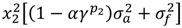 + [(1 − ω)p1x1)]2[
 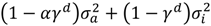 ].
].
Var[w|s], where E[w|s] = x2 (m + γd s) + ωp1x1 (1 + rf) + (1 − ω)p1x1(m + γd s) and Var[w|s] = + [(1 − ω)p1x1)]2[ ].3.1. First Order Conditions
The first order conditions associated to the maximization problem (7) yield:
 where x2 is given by (1).
Notice that, ∂x2/∂x1 < 0, (9) holds only if 
3.1.1. Harvesting and Investment
When analyzing the relationship between the optimal short-run supply of timber, x1, and the financial portfolio (ϖ, 1 − ϖ), it is easy to notice that the investment in the risky asset (1 − ϖ)p1x1 is not affected by the specific level of current harvesting x1. Hence, if harvesting is increased at time 1, the extra-revenues from timber sales are invested into the risk-free asset, and not in the risky one. In a similar fashion, as long as the signal on the financial market is observable, even if the landowner was given the possibility to exclusively invest in the risk-free asset [28], the optimal short-run supply of wood would be given by the same x1 solving (9) [29].
In general, there is a trade-off between investing in the risk-free asset and allowing the forest to grow to time 2. This immediately appears in the first order condition (9): If m falls, x1 (harvesting in the first period) increases and the total investment in the risk-free asset increases as well. Similarly, if p1 or rf increases, so do x1 and the investment in the risk-free asset.
3.1.2. Harvesting and Risk
The increase in aggregate economic risk and in the two idiosyncratic risks impacts the short-run supply of timber (x1), and therefore investment. In particular, if risk in the forest sector σf2 increases, so does current harvesting x1 and the investment in the risk-free asset, as can be expected. Similarly, if risk-aversion ρ increases, so does x1. The investment in the risk-free asset increases as well, but this time also because the investment in the risky asset (1 − ϖ) is reduced by the increase in risk-aversion.
Inspection of the first order condition (9) reveals an interesting result: when the asset specific risk σi2 increases, this is transmitted to the optimal harvested quantity through the signal s. In particular, the signal's informativeness is reduced as reflected in the decrease of γp2. If the signal conveys good news, a higher financial risk σi2 unequivocally increases short-run timber supply, ceteris paribus. In case of a negative signal, instead, the effect is a priori ambiguous [30]. However, for high risk aversion, again short run supply increases when asset specific risk increases, ceteris paribus.
The effect of financial risk σi2 on optimal harvesting is due to the presence of the common aggregate economic component εa and the signal s on the asset's dividend. Further, as noted above, under these assumptions financial risk σi2 affects optimal harvest as long as the agent observes the signal, no matter if he is given the actual possibility to invest in the risky asset or not. On the contrary, if no signal was received, and/or p2, s and d had no common component, the first order condition associated to the optimal harvesting quantity would not depend on σi2.
To the best of our knowledge, our model is the first in the literature to suggest that financial idiosyncratic risk can have an impact on harvesting behavior. Despite the relative difficulty in providing an accurate empirical analysis of this claim, the observation of the patterns followed by timber markets during, in particular, the first phase of the recent financial downturn might support this idea, as discussed in more detail in Section 4.
Finally, it is interesting to notice how harvesting and financial investment react differently to an increase in aggregate economic risk. For simplicity, consider the case α = 1. An increase in the aggregate economic risk σa2 will always reduce the investment in the risky asset (1 − ϖ), no matter what the realization of the signal and the level of risk-aversion ρ are. The reaction of the harvesting schedule is instead ambiguous for a positive signal and it depends on risk-aversion, ρ [31] , if ρ is quite low, an increase in aggregate economic risk could possibly lead to a reduction in current harvesting level x1 [32].
This result indicates that the forest owner is behaving differently when deciding about timber harvesting compared to the evaluation of financial assets. In particular, let us consider an alternative risky asset at the place of the forest, with dividend d = p2. The first order condition associated to this problem shows that, in case of a positive signal, the variation of the investment in the second asset in response to an increase in σa2, is ambiguous, but in this case the sign of the reaction depends on the relative magnitude of variances, expected dividend, risk-free rate and signal realization, but not on the level of risk-aversion.
Even if it is beyond the scope of this paper to empirically evaluate the validity of the framework proposed, these findings seem to suggest that timber prices and financial markets co-move in quite a complicated manner, presenting both significant and negligible correlation; as empirical evidence from the literature also seems to suggest (see Section 4).
3.1.3. Harvesting and the Signal Realization
We next investigate how harvesting is affected by the “positivity” of the information conveyed by the signal.
Suppose that s = 0, so that the updated expected dividend and timber price after having observed the signal do coincide with the unconditional ones, namely, E[d|s] = m, and E[p2|s] = m.
Let us denote by x1° the solution to (9) when the realization of the signal is s = 0.
Next, we define the function ϕ(x1,s), such that ϕ(m,x1,s,α,ρ,p1,rf)=  × (m + γp2s − ρx2[
 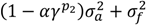 ]) + p1(1 + rf). Hence, ϕ(m,x1°,s,α,ρ,p1,rf) = 0.
× (m + γp2s − ρx2[ ]) + p1(1 + rf). Hence, ϕ(m,x1°,s,α,ρ,p1,rf) = 0.An increase of the signal to s > 0 (that is, the arrival of good news) translates into ϕ(m,x1°,s,α,ρ,p1,rf) < 0. Since, ∂x2/∂x1 < 0 and ∂2x2/∂2x1 < 0, the new equilibrium requires a lower x1, so that the short-run supply of wood is reduced. As a consequence, also the total investment in the financial market p1x1 is reduced. In addition, given the positivity of the signal, the investment portfolio (ϖ, 1 − ϖ) is tilted towards the risky asset.
Summarizing, the arrival of good news induces a reduction in current harvesting (which in turn translates in a decrease of current wealth) and in the proportion of current wealth invested in the risk-free bond in favor of the one in the risky investment. The opposite happens if the signal conveys bad news (that is if s < 0); in this particular instance, harvesting at time 1 is increased, and the financial portfolio is tilted towards the risk-free asset.
3.2. Information
The informativeness of the signal depends on risks σa2, σi2, precision σs2, and the specificity parameter, α. Higher precision (i.e., lower σs2) translates into higher informativeness for both the dividend and the price. Hence, the new equilibrium requires a lower x1 and an investment portfolio more tilted towards the risky investment (that is, higher (1 − ϖ)). Therefore the investment in the risk-free asset is reduced because of the reduction of x1, but also because of the change in the optimal portfolio composition.
If good news arrives (s > 0), short-run supply reduces as α increases [33]. This simply means that the more the signal becomes informative about aggregate economic risk, the stronger the forest landowner reacts to it (reducing the short-run supply of wood). In case of a negative signal the result is ambiguous: on one side a very trustable negative signal would induce an increase in the current-supply of wood. On the other hand, the fact that the signal is less specific to financial markets reduces the conditional variance of future timber price (i.e., its overall risk), and consequently short-run supply is reduced.
3.2.1. Information Specific to the Timber Market
In the following we assume that the signal, s, concerns the price of timber at time 2. In particular,
s = αεa + εf + εs
If α = 0, the signal exclusively brings information about the timber price, and it cannot be used to infer any information about the financial market. The first order condition for harvesting associated to the maximization problem yields:
 where x2 is given by (1).
As before, since ∂x2/∂x1 < 0, the first order condition associated to optimal harvesting holds only if  .
.
.Using this alternative formulation, one obtains that σf2 affects the optimal investment in the financial asset while the specific financial risk σi2 has no influence on the harvest level.
To facilitate the analysis, let us here assume that σi2 = σf2. When comparing (9) and (11), the role played by the degree of informativeness of the signal immediately becomes apparent. In particular, as is intuitive, a positive signal induces a higher reduction in the short-run supply of wood when the signal itself is supposed to be informative about the forest sector, as it is in (11).
This does not immediately follow in the case of a negative signal: on the one hand a very trustable negative signal would induce an increase in the current-supply of wood. On the other hand, the high degree of informativeness is perceived as a reduction in risk and therefore it reduces current supply x1. In particular, for higher levels of risk aversion this second effect could prevail.
Comparative statics with respect to the parameters m, s, α, ρ, α, σa2, σf2, σs2, rf and p can be carried out as in the previous case.
3.2.2. The Importance of Information
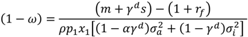
In this section, we briefly discuss the role played by the signal when the information conveyed does not add anything with respect to the initial expectations. This occurs when the realized signal (on the risky asset or on future timber price) takes value 0. In such an instance, the first order condition for optimal harvesting associated to the maximization problem will be:
 if the signal is related to the financial market, and:
 if the signal is specific to the forest sector.
We label the solution of the above equations x1A and x1B, respectively. We denote by x1 the optimal solution if no signal is received, and, to facilitate the comparison, we assume σi2 = σf2. Even if the updated expectations have not changed, the mere existence of the signal has strong impact on the optimal harvesting/investment quantities, through the reduced conditional variance, and therefore risk. In particular, x1B < x1A < x1, that is, the more the signal is specific to the forest sector, the more it reduces uncertainty. Notice that this implies that different landowners could react to the same signal in different ways, depending on whether they consider the signal more related to the forest sector or to financial markets. The difference |x1A − x1| reduces as σi2, σf2 increase, while it increases as α and σa2 increase.
Therefore, the reply to the signal is stronger the higher the aggregate economic risk σa2 is, and the more informative the signal is. In contrast, σf2 and σi2 reduce the credibility of the signal. Indeed, when aggregate economic risk is high, it is relatively more important for the forest owner to receive a signal, so that he/she tends to “over-react” with respect to it. On the other hand, financial risk and the signal precision do not directly affect timber prices, which is why their increase simply adds disturbance to the interpretation of the signal, so that the forest owner becomes more cautious.
It is also worth noting that—even if in both cases considered above, the signals bring the same information about the economic component—the reaction to the signal of the second agent is stronger, simply because informativeness itself is stronger [34].
4. Discussion and Conclusions
In this paper we have presented a theoretical model of optimal harvesting-investment decision for a private forest owner who invests the revenues from timber sale on financial markets. The framework has two main characteristics: (i) the role of information and (ii) the way uncertainty is modeled. As far as it has been possible to ascertain, this is the first theoretical paper investigating the effect of information on harvesting decisions. When modeling uncertainty, we explicitly allow for a distinction between aggregate economic risk and sector specific risk, such as financial and forestry risk respectively. Obviously it is beyond the scope of this paper to try to establish a direct linkage between concrete empirical facts and the results of our model. Nevertheless, the particular structure used here permits financial specific risk to influence harvesting behavior (see Section 3.1.2 above), and, along with the introduction of the information component, it furthers the understanding of recent trends in timber prices that are difficult to explain using standard models.
For example, when the housing sector collapsed in US, timber prices in Sweden plummeted dramatically, as expected. However, they dropped even further after Lehman Brothers’ bankruptcy [16]. To make a parallelism with the framework presented above, the Lehman Brothers’ breakdown could be interpreted as the “arrival of a signal”, carrying information on both aggregate economic and financial risk, affecting economic operators (including those in the forest sector) all over the world. Indeed, though the growth forecasts had already been gradually corrected downward since August 2007 [17], they dropped dramatically only with the collapse of Lehman Brothers’, an event which apparently took market participants by surprise and therefore induced a strong reaction in prices.
The presence of common aggregate economic risk (due to the potential occurrence of a shock, εa) and the arrival of financial information make the way financial and timber markets interact non-trivial, reconciling the mixed empirical evidence reported in the literature. Indeed, there is no consensus on the way timber prices and financial markets co-move. On one side, some studies have found a positive correlation between timber and financial markets [20,21], while quite a few studies point out that forest investments are an attractive alternative for risk diversification, due to negligible correlation with financial assets (see, e.g., [22,23,24]).
Even if ours is not an equilibrium model, so that both financial and timber prices are exogenous, observing the conditional covariance between timber price and asset dividend one could partially accommodate these contrasting findings. Indeed, conditional covariance varies in value depending on the severity of aggregate economic risk and the specific information received (see Section 2.2). Finally, Heikkinen [21]—using time series data for the period from January 1988 to September 1999—finds that the correlation between timber and financial markets increases over time. This finding seems to be consistent with the idea that harvesting decision-making adjusts to the arrival of new information. This is also why we contend that the role of information in harvesting decision should be further investigated.
The accommodation of the role played by information/news in the model—particularly information specific to timber markets—is of relevance from a policy perspective. Hence, information is a frequently used policy tool, and the way information affects harvesting decisions is thus of interest, especially in light of the efforts to increase wood mobilization in many European countries. As an example, information about timber markets, coupled with recommendations not to postpone harvest, features frequently in forest owner associations membership magazines, presumably partly with the objective to increase the short-run supply of timber (see, e.g., [18]).
Thus the model presented here can be used as a starting point for exploring an area of forest economics well worth considering, not least from a policy perspective and with very concrete applications. For example, departing from the approach proposed here, it is possible to develop an alternative framework suitable for analyzing how different degrees of information penetration affect the equilibrium price of timber. Alternatively, one could investigate how the release of information could be used as a policy tool to optimally induce higher/lower levels of timber supply among forest owners, depending on their specific characteristics (e.g., stand characteristics related to the extent of non-timber forest values). These topics will be part of our future research.
Conflicts of Interest
The authors declare no conflict of interest. The opinions expressed herein are those of the authors and do not necessarily reflect the views of the European Commission.
References and Notes
- State of Europe’s Forests 2011: Status and Trends in Sustainable Forest Management in Europe; FOREST EUROPE/FAO/UNECE, Ministerial Conference on the Protection of Forests in Europe, FOREST EUROPE Liaison Unit: Oslo, Norway, 2011. Available online: http://www.unece.org/fileadmin/DAM/timber/soef/SoEF2011_revised_version_november.pdf (accessed on 2 October 2013).
- Stern, T.; Schwarzbauer, P.; Huber, W.; Weiss, G.; Aggestam, F.; Wippel, B.; Petereit, A.; Navarro, P.; Rodriguez, J.; Boström, C.; de Robert, M. Identifying practices and policies for wood mobilisation from fragmented forest areas. Ökosystemdienstleistungen und Landwirtschaft. Herausforderungen und Konsequenzen für Forschung und Praxis. 22. Jahrestagung der Österreichischen Gesellschaft für Agrarökonomie. Universität für Bodenkultur: Vienna, Austria, 2012; pp. 119–120. Available online: http://oega.boku.ac.at/fileadmin/user_upload/Tagung/2012/OEGA_TAGUNGSBAND_2012.pdf (accessed on 2 October 2013).
- Kuuluvainen, J.; Karppinen, H.; Ovaskainen, V. Landowner objectives and nonindustrial private timber supply. For. Sci. 1996, 42, 300–309. [Google Scholar]
- Johansson, P.O.; Löfgren, K.G. The Economics of Forestry and Natural Resources; Basil Blackwell: Oxford, UK, 1985. [Google Scholar]
- Koskela, E. Forest taxation and timber supply under price uncertainty: Perfect capital markets. For. Sci. 1989, 35, 137–159. [Google Scholar]
- Koskela, E. Forest taxation and timber supply under price uncertainty: Credit rationing in capital markets. For. Sci. 1989, 35, 160–172. [Google Scholar]
- Ollikainen, M. Forest taxation and the timing of private nonindustrial forest harvests under interest rate uncertainty. Can. J. For. Res. 1990, 20, 1823–1829. [Google Scholar] [CrossRef]
- Ollikainen, M. A mean-variance approach to short-term timber selling and forest taxation under multiple sources of uncertainty. Can. J. For. Res. 1993, 23, 573–581. [Google Scholar] [CrossRef]
- Uusivuori, J. Nonconstant Risk Attitudes and Timber Harvesting. For. Sci. 2002, 48, 459–470. [Google Scholar]
- Gong, P.; Löfgren, K.G. Risk-aversion and the short-run supply of timber. For. Sci. 2003, 49, 647–656. [Google Scholar]
- Caulfield, J.P. A stochastic efficiency approach for determining the economic rotation of a forest stand. For. Sci. 1998, 34, 441–457. [Google Scholar]
- Taylor, R.G.; Fortson, J.C. Optimum planting density and rotation age based on financial risk and return. For. Sci. 1991, 37, 886–902. [Google Scholar]
- Valsta, L.T. A scenario approach to stochastic anticipatory optimization in stand management. For. Sci. 1992, 38, 430–447. [Google Scholar]
- Gong, P. Risk preferences and adaptive harvest policies for even-aged stand management. For. Sci. 1998, 44, 496–506. [Google Scholar]
- We emphasize that this is a key distinctive element between [8] and [10], since the latter assumes distributional independence, while the former bases its results specifically on correlation.
- Dramatiskt ras på virkespris; Dalanytt: Falun, Sweden, 2009. Available online: http://sverigesradio.se/sida/artikel.aspx?programid=161&artikel=2683304 (accessed on 2 August 2013).
- Prakash, K.; Koehler-Geib, F. The Uncertainty Channel of Contagio; IMF Working Papers 4995; The World Bank, Poverty Reduction and Economic Management Network, Economic Policy and Debt Department: Washington, DC, USA, 2009; p. 36. [Google Scholar]
- Södrakontakt nr.4; Södrakontakt: Växjö, Sweden, 2013. Available online: http://skog.sodra.com/Documents/Tidningar%20och%20informationsblad/Södrakontakt/2013/Södrakontakt%20nr%204%202013.pdf (accessed on 1 September 2013).
- Serbruyns, I.; Luyssaert, S. Acceptance of sticks, carrots and sermons as policy instruments for directing private forest management. For. Policy Econ. 2006, 9, 285–296. [Google Scholar] [CrossRef]
- Heikkinen, V.-P.; Kanto, A. Market model with long-term effects—Empirical evidence from Finnish forestry returns. Silva Fenn. 2000, 34, 61–69. [Google Scholar]
- Heikkinen, V.-P. Co-integration of timber and financial markets—Implications for portfolio selection. For. Sci. 2002, 48, 118–128. [Google Scholar]
- Lönnstedt, L.; Svensson, J. Return and risk in timberland and other investment alternatives for NIPF owners. Scand. J. For. Res. 2000, 15, 661–669. [Google Scholar] [CrossRef]
- Penttinen, M.; Lausti, A. The Competitiveness and return components of NIPF ownership in Finland. The Finn. J. Bus. Econ. 2004, 2, 143–156. [Google Scholar]
- Healey, T.; Corriero, T.; Rozenov, R. Timber as an institutional investment. J. Altern. Invest. 2005, 8, 60–74. [Google Scholar] [CrossRef]
- In what follows we will use the terms “agent”, “individual” and “landowner” interchangeably, without special or technical meanings, unless otherwise stated.
- The case of a signal on the forest sector will be treated in a separate section.
- CARA (constant absolute risk aversion) utility is a class of utility functions u(w) characterized by the property that the associated risk aversion coefficient usually defined as − u′′(w)/u′(w) is a constant parameter and does not vary with the wealth level.
- In such an instance, final wealth would be w = p2x2 + p1x1 (1 + rf).
- We refer the Reader to the next section in order to obtain additional insight on this result.
- Indeed higher risk makes the signal less credible and the absolute value of the variation in the short-run timber supply induced by an increase in financial risk is higher in case of good news.
- Indeed
 .
. - In the case of a negative signal, current harvesting always increases with economic risk.
- Notice that we are implicitly assuming that ∂γp2/∂α > 0, that is σa2α2 ≤ σi2 + σs2, which is generally the case for realistic values of σa2, α, σi2, σs2.
- Here we are evaluating |x1A − x1B|.
© 2013 by the authors; licensee MDPI, Basel, Switzerland. This article is an open access article distributed under the terms and conditions of the Creative Commons Attribution license (http://creativecommons.org/licenses/by/3.0/).