Retrieval of Mangrove Leaf Area Index Using Multispectral Vegetation Indices and Machine Learning Regression Algorithms

Abstract

Leaf Area Index (LAI) is the total leaf area per unit of land surface area and is a crucial parameter for assessing vegetation growth and productivity. Machine learning regression algorithms are widely applied for LAI estimation. Due to spectral response variations among sensors and susceptibility of mangrove-derived variables to environmental noise suppression, obtaining sensitivity indices and optimal machine learning regression models is essential for retrieving mangrove LAI at the population scale. This study proposes a novel approach to processing and retrieving mangrove LAI data by integrating multispectral indices with machine learning methods. Box–Cox transformation and CatBoost-based feature selection were employed to obtain the optimal dataset. Random Forest (RF), Gradient Boosting Regression Trees (GBRT), and Categorical Boosting (CatBoost) algorithms were used to evaluate the accuracy of LAI retrieval from Unmanned Aerial Vehicle (UAV) and Gaofen-6 (GF-6) data. Results indicate that when LAI > 3, LAI does not immediately saturate as CVI, MTVI 2, and other indices increase, demonstrating higher sensitivity. UAV data outperformed GF-6 data in retrieving LAI for diverse mangrove populations; during model training, RF proved more suitable for small-sample datasets, while CatBoost effectively suppressed environmental noise. Both RF and CatBoost demonstrated higher robustness in estimating Avicennia marina (AM) (RF: R² = 0.704) and Aegiceras corniculatum (AC) (R² = 0.766), respectively. Spatial distribution analysis of LAI indicates that healthy AM and AC cover 85.36% and 96.67% of the area, respectively. Spartina alterniflora and aquaculture wastewater may be among the factors affecting the health of mangrove forests in the study area. LAI retrieval holds significant importance for mangrove health monitoring and risk early warning.

1. Introduction

Mangroves are intertidal wetland ecosystems unique to tropical and subtropical regions, providing vital ecological services to coastal areas and playing a crucial role in establishing and stabilizing coastlines [1,2]. However, multiple pressures, including human activities, climate change, and mismanagement, threaten global mangrove resources. Coastal fishing and aquaculture activities not only lead to overharvesting of selected mangrove species but may also cause habitat destruction, posing potential threats to the long-term health of mangrove ecosystems [3]. Secondly, natural disturbances such as pests, diseases, and invasive species like Spartina alterniflora inhibit mangrove growth [4]. The health status of mangrove ecosystems therefore warrants increasing attention, highlighting the need for effective, quantitative, and scalable monitoring approaches to support mangrove conservation and sustainable management.

Physiological and structural parameters, as key factors in assessing plant health and adaptability, are crucial for understanding mangrove ecosystem health. Currently, methods for extracting vegetation LAI primarily include ground-based measurements and remote sensing inversion techniques. Traditional LAI measurements rely heavily on ground surveys, but this approach is often time-consuming, destructive to vegetation, and impractical for obtaining LAI information over large areas [5]. Previous research has demonstrated that vegetation indices and parameters extracted from remote sensing data sets can effectively characterize mangrove health, such as LAI and chlorophyll concentration [6]. In remote sensing inversion studies of mangrove LAI, multispectral sensors, hyperspectral sensors, and LiDAR point clouds have been proven effective methods [7]. Low-resolution satellites like MODIS and medium-to-high-resolution satellites such as Sentinel-2 are widely applied for LAI estimation at various scales [8]. Multispectral satellite data like Sentinel-2 can overcome the extensive reliance on in situ measurement training data found in other methods, demonstrating broader applicability in mangrove LAI inversion and thus being widely adopted [9]. Hyperspectral data, such as Zhuhai-1, feature numerous narrow bands, which have been shown through radiative transfer model-based analysis to exhibit high sensitivity to LAI [10]. In studies using optical data for LAI inversion, Zhao (2023) [11] compared the LAI estimation capabilities of Landsat-8, Sentinel-2, Worldview-2, and Zhuhai-1 data. These studies show that spatial and spectral resolution significantly impact the mapping accuracy of mangrove LAI, with imagery featuring higher spectral or spatial resolution demonstrating greater robustness in LAI inversion. Compared to optical data, LiDAR possesses the capability to penetrate vegetation canopies, is less affected by understory coverage, and can finely delineate upper and lower canopy structures [12]. For high-precision estimation of mangrove population LAI, the spatial resolution of remote sensing imagery becomes critical.

In contrast to traditional satellite remote sensing, UAV offer greater flexibility and controllability in flight altitude, observation angle, heading, and fore-and-aft overlap. Unlike satellites, they do not require consideration of revisit cycles, allowing missions to be flexibly adjusted according to tidal changes. UAV data can effectively overcome interference from complex backgrounds and multiple vegetation species [13,14]. Compared to satellite remote sensing, UAV have a smaller flight range. High-resolution multispectral satellite data from Gaofen-6 can achieve 2 m spatial resolution through data fusion. Its wavelength range aligns with UAV data and has been effectively applied in estimating canopy chlorophyll content in mangrove populations, compensating for the limited mapping scope of UAV [15]. In LAI retrieval, increasing recognition exists among scholars regarding the spatial and textural advantages of satellite-borne and aerial high-resolution imagery. However, the consistency and complementarity of UAV ultra-high-resolution imagery and GF-6 high-resolution satellite data for mangrove stand LAI estimation remain insufficiently explored, particularly across different spatial scales.

Deriving sensitivity parameters from satellite sensors facilitates the retrieval of mangrove LAI. These remote sensing image parameters typically include bands or their spectral transformations, texture information, backscatter coefficients, and others [16]. For instance, in estimating vegetation parameters using optical sensors, Heenkenda (2015) [17] proposed that reflectance around 550 nm or within the 680–750 nm range provides highly accurate indicators for predicting mangrove chlorophyll content. Among spectral transformation methods, vegetation indices are most frequently employed. Currently, the most widely applied approach for LAI estimation combines visible and near-infrared vegetation indices [18,19]. Zhao (2023) demonstrated that vegetation indices constructed using the 443–908 nm wavelength range effectively estimate mangrove LAI [11]. Tran (2022) [20] investigated spectral indices and found that the Normalized Difference Vegetation Index (NDVI) is the most widely applied for estimating mangrove aboveground parameters (e.g., carbon density, biomass, canopy height, and LAI), followed by the Enhanced Vegetation Index (EVI. Manna (2020) [21] demonstrated that composite NDVI (NDVI_com) is more sensitive to LAI, yielding improved LAI estimates. Compared to single indices, multi-index parameters reflect diverse spectral characteristics, thereby enhancing sensitivity to LAI. Fu (2022) [7] incorporated multiple vegetation indices (NDVI, RVI, ARVI, SAVI, EVI, etc.) into various regression models to achieve superior LAI estimation capabilities. In particular, species-specific differences in vegetation index sensitivity for LAI retrieval using combined UAV and GF-6 data have not yet been systematically evaluated in mangrove ecosystems.

Currently, remote sensing inversion methods for vegetation parameters primarily include parametric regression (VIs), nonparametric regression (linear regression, ridge regression, etc.), and nonlinear regression (such as machine learning regression and artificial neural network regression) [22]. Juniansah (2018) [23] established an optimal parametric regression model for mangrove LAI based on the strong correlation between NDVI and EVI indices and field-measured LA. Li (2020) [24] estimated effective understory vegetation LAI (Leo), understory vegetation LAI (Leu), and total LAI (Let) using parametric and nonparametric regression methods. Findings indicated that nonparametric regression typically yielded the highest accuracy and effectively handled composite data. Gaussian process regression (GPR), as a nonparametric regression method, has proven to be a proficient time series processor capable of Green LAI mapping across global scales [25]. Machine learning regression algorithms (MLA), as nonlinear regression methods, can balance errors across datasets and exhibit strong model generalization capabilities. Their ability to establish adaptive and robust relationships between input and output data makes them effective for simulating vegetation parameters using both remote sensing and field measurement data [22,26,27]. Heenkenda (2015) [17] employed a nonlinear random forest approach to characterize the relationship between mangrove canopy chlorophyll and remote sensing datasets while estimating the spatial distribution of vegetation canopy chlorophyll variation. Lou (2021) [28] demonstrated that adjusting parameters within a single RF model significantly improves the accuracy of GF-1 WFV, Landsat-8 OLI, and Sentinel-2 MSI sensors in determining canopy chlorophyll content over marsh wetlands, with particularly notable enhancements for Sentinel-2 MSI. Given that different models possess distinct assumptions and data fitting capabilities, comparative analysis can identify the most suitable model to enhance LAI inversion accuracy. Miao (2022) [29] compared three machine learning regression models—RF, XGBoost, and LightGBM—and concluded that XGBoost, utilizing sensitive spectral features from Sentinel-2 imagery, provided the optimal estimation of leaf carbon, nitrogen, and phosphorus in mangroves. Deng (2023) [15] constructed optimal canopy chlorophyll content models for different mangrove species by comparing RF, GBRT, and XGBoost algorithms, while also noting that XGBoost exhibited overfitting when training datasets were insufficient. The CatBoost algorithm incorporates an algorithm for selecting leaf nodes in tree structure construction, thereby mitigating overfitting [30,31]. Therefore, a systematic comparison of machine learning regression models, including RF, GBRT, and CatBoost, for species-specific mangrove LAI estimation using multi-source remote sensing data is still lacking.

The objectives of this study are to: (1) evaluate and compare the performance of multispectral UAV imagery and GF-6 satellite data for stand-level mangrove leaf area index (LAI) estimation; (2) assess the applicability of different vegetation indices and machine-learning regression models, including Random Forest (RF), Gradient Boosting Regression Tree (GBRT), and CatBoost gradient boosting decision trees, for LAI retrieval in Avicennia marina and Aegiceras corniculatum; and (3) examine how sensor characteristics, particularly spatial and spectral resolution, together with model performance, influence the accuracy of LAI estimation, and how LAI spatial distribution patterns reflect mangrove habitat conditions. This study integrates multispectral vegetation indices derived from UAV imagery and GF-6 data with machine-learning algorithms calibrated against field-measured LAI, aiming to systematically compare LAI retrieval performance across sensors and species and to provide a methodological reference for multi-source remote sensing applications in mangrove canopy-scale analysis.

2. Materials and Methods

2.1. Study Area and Species

The study area is located in the mangrove wetland along the Dafeng River in the Beibu Gulf, Guangxi. The entire plot is designated as SJ (Figure 1), with geographic coordinates ranging from 108°48′15″ E to 108°52′15″ E and 21°37′00″ N to 21°38′20″ N. This area exhibits a typical subtropical monsoon maritime climate, providing excellent natural conditions for mangrove growth. The study area is dominated by populations of Avicennia marina (AM), and Aegiceras corniculatum (AC), with AM covering a larger area than AC. Human activities are prominent in the study area, with extensive invasions of Spartina alterniflora occurring seaward. Concurrently, mangrove ecosystems face threats from pest and disease pressures, jeopardizing their ecological health [4]. Obtaining spatial distributions of LAI in this region is crucial for monitoring mangrove health.

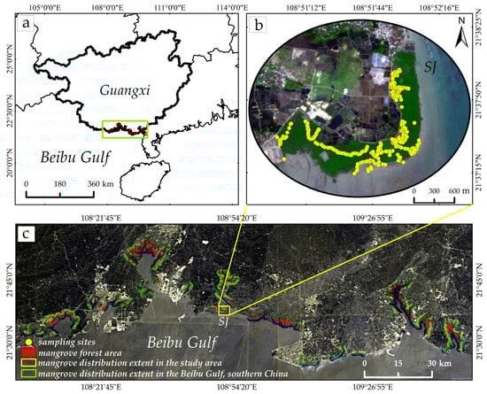
Figure 1. Location of study area and sampling sites. (a) Location of the study area in Guangxi Province and the Beibu Gulf; (b) Distribution of field sampling sites overlaid on Sentinel-2 imagery in the Shajiao (SJ) mangrove area; (c) Spatial distribution of mangrove forests within the study area and across the broader Beibu Gulf region.

2.2. LAI In Situ Measurement and Image Processing

2.2.1. Field Measurements

To obtain accurate in situ LAI data, we collected 85 AM plots and 62 AC plots within the study area from 8 January 2021 to 6 April 2021. Field plots were established within representative mangrove stands following a stratified sampling design, and adjacent plots were separated by distances exceeding the spatial resolution of the GF-6 imagery to reduce spatial autocorrelation and mixed-pixel effects. Specific requirements for data collection were as follows: (1) To minimize human interference, survey sites were located 30 m inland from the coastline; (2) Each plot size was kept as close as possible to a 10 m × 10 m square, as previous studies have shown that 10 m × 10 m plots are the optimal scale for estimating LAI [16,32]; (3) LAI data for mangroves were measured using the LAI-2200 canopy analyzer (LI-COR Biosciences Inc., Lincoln, NE, USA) (Table 1), and the geographic coordinates of each plot were recorded using the CNOOC V90 GNSS RTK system (CHCNAV, Shanghai, China). All field LAI measurements were conducted under rain-free conditions and during periods of lowest tide to ensure that mangrove canopies were not flooded.

Table 1. Summary statistics of measured LAI for AM and AC mangrove species.

Species	Number of Samples	Mean Value	Standard Error of Mean	LAI Range
AM	85	1.87	0.05	[0.93, 3.04]
AC	62	2.60	0.08	[1.26, 4.03]

2.2.2. UAV and GF-6 Multispectral Data Processing

While collecting ground sample plots, the experiment simultaneously deployed a DJI Matrice 210 (M210) drone (DJI, Shenzhen, China). This drone was equipped with a MicaSense RedEdge™ (MicaSense, Inc., located in Seattle, Washington, DC, USA), providing multispectral bands: blue (band 1: 460–510 nm), green (band 2: 545–575 nm), red (band 3: 630–690 nm), red edge (band 4: 712–722 nm), and near-infrared (band 5: 820–860 nm). During flight, the altitude is set to 100 m, with both heading and sideways overlap rates set to 80%. UAV flights were conducted under rain-free conditions and during periods of lowest tide, consistent with field LAI measurements. The original UAV imagery was recorded as digital number (DN) values and radiometrically calibrated using a reflectance panel, with the corresponding reflectance coefficients input into Pix4D 4.5.6 to convert DN values to surface reflectance. Using the Georeferencing Toolbar in ArcMap 10.8, the imagery was georeferenced to the WGS 1984 UTM Zone 49N coordinate system, achieving a root mean square error (RMSE) of 0.21. Non-mangrove areas were subsequently masked.

The selection of the Gaofen-6 (GF-6) image was constrained by the satellite revisit cycle and data availability and represents the closest cloud-free observation temporally matched to the UAV flights and field surveys. GF-6 imagery was also acquired under rain-free and low-tide conditions. GF-6 satellite is a low-orbit optical remote sensing satellite and China’s first high-resolution satellite dedicated to precision agriculture observation. GF-6 satellite data is acquired through the https://data.cresda.cn (accessed on 12 September 2022) (CRSC), with imagery captured on 2 January 2021. Equipped with an 8-band CMOS sensor, GF-6 captures imagery at 2 m panchromatic and 8 m spatial resolutions. It provides blue (band 1: 450–520 nm), green (band 2: 520–600 nm), red (band 3: 630–690 nm), near-infrared (band 4: 760–900 nm), and Pan (p: 450–900 nm). The GF-6 data were preprocessed using radiometric calibration and atmospheric correction to convert DN values to surface reflectance prior to analysis. The multispectral and panchromatic bands were georeferenced using GNSS RTK positioning data with the Georeferencing Toolbar in ArcMap 10.8, achieving registration errors of 0.32 and 0.38, respectively. The bands were then fused into 2 m-resolution multispectral imagery using the Gram–Schmidt pan-sharpening tool in ENVI 5.6, and non-mangrove surfaces were simultaneously masked.

2.3. LAI Modeling Framework and Accuracy Assessment

This study employs UAV and GF-6 multispectral data, integrating RF, GBRT, and CatBoost algorithms to estimate LAI for mangrove species AM and AC. The methodology is as follows: (1) Preprocess UAV and GF-6 multispectral data to obtain ground-truth reflectance information while performing spectral transformations to calculate vegetation indices; (2) Optimal parameters were selected through normality tests, correlation analysis, BOX-COX transformations, and feature variable selection; (3) Incorporate the optimized variables into RF, GBRT, and CatBoost machine learning regression models for training and prediction using ground-truth measurements; (4) Perform RF classification of the study area to delineate the distribution ranges of different tree species; (5) Generate LAI maps based on mangrove species distribution information and the index parameter model (Figure 2).

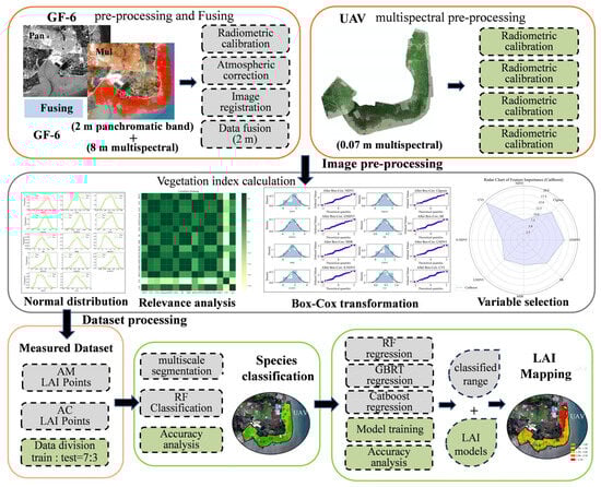
Figure 2. Technology roadmap for LAI mapping.

2.3.1. Calculation of the Vegetation Index

The effects of soil background and shading in traditional band reflectance measurements of mangrove growth areas were mitigated or eliminated by calculating vegetation indices. Through spectral transformations of two-band and three-band data, this study computed 14 vegetation indices for both the UAV and GF-6 datasets (Table 2). The vegetation index calculations were performed using the Band Math tool in ENVI 5.6 software.

Table 2. Selected multispectral indices for LAI retrieval derived from UAV and GF-6 data.

Multispectral Index	Formula	Reference
NDVI	$({\rho }_{nir}-{\rho }_{red})/({\rho }_{nir}+{\rho }_{red})$	[33]
GNDVI	$({\rho }_{nir}-{\rho }_{green})/({\rho }_{nir}+{\rho }_{green})$	[34]
LNDVI	$1.2\times ({\rho }_{nir}-{\rho }_{red})/({\rho }_{nir}+5\times {\rho }_{red})$	[35]
S-NDVI	$4/\left(1+2\times \left(1.2/NDVI\right)\right)$	[36]
EVI	$2.5\times ({\rho }_{nir}-{\rho }_{red})/({\rho }_{nir}+6\times {\rho }_{red}-7.5\times {\rho }_{blue}+1)$	[37]
EVI2	$2.5\times ({\rho }_{nir}-{\rho }_{red})/({\rho }_{red}+2.4\times {\rho }_{red}+1)$	[38]
SR	${\rho }_{nir}/{\rho }_{red}$	[39,40]
MSR	$({\rho }_{nir}/{\rho }_{red}-1)/SQRT({\rho }_{nir}/{\rho }_{red}+1)$	[41,42]
CIgreen	${\rho }_{nir}/{\rho }_{green}-1$	[43,44]
CVI	$({\rho }_{nir}\times {\rho }_{red})/({{\rho }_{green}}^2)$	[45,46]
MSAVI	$\begin{array}{l}(2{\rho }_{nir}+1-SQRT({(2{\rho }_{nir}+1)}^2- 8 \times ({\rho }_{nir}-{\rho }_{red}))\hfill \end{array})/2$	[47]
MTVI2	$1.5\times (1.2\times ({\rho }_{nir}-{\rho }_{green})-2.5\times ({\rho }_{red}-{\rho }_{green}))/SQRT({(2\times {\rho }_{red}+1)}^2-(6\times {\rho }_{nir}-5\times SQRT({\rho }_{red}))-0.5)$	[41]
RDVI	$({\rho }_{nir}-{\rho }_{red})/SQRT({\rho }_{nir}+{\rho }_{red})$	[41,48]
SAVI	$\left(1+0.5\right)\times ({\rho }_{nir}-{\rho }_{red})/({\rho }_{nir}+{\rho }_{red}+0.5)$	[49]

Note. ρ represents the reflectance at a given spectral band. Central wavelengths of the UAV bands are blue (485 nm), green (560 nm), red (660 nm), and near-infrared (nir: 840 nm). For the GF-6 multispectral data, the corresponding band-center wavelengths are blue (485 nm), green (560 nm), red (660 nm), and near-infrared (nir: 830 nm).

2.3.2. Construction of Machine Learning Regression Algorithms (MLAs)

Random Forest (RF) is a highly representative Bagging ensemble algorithm, where all underlying evaluators are decision trees. Its primary purpose is to predict new data points through voting [50]. Its prediction process primarily involves Bootstrap Sampling, Building Multiple Trees, Independent Training, and Aggregating Predictions, culminating in the output of a final prediction. For regression tree forests, the prediction result is typically formed by averaging the individual predictions [51,52].

Gradient Boosting Regression Trees (GBRT) is an algorithm based on gradient boosting that uses decision trees as its base learners. GBRT integrates multiple regression variables into a robust regression algorithm. Its core principle is to construct new regression trees based on the results of previous trees, following the direction that minimizes the gradient of the loss function [53]. The GBRT prediction process differs significantly from RF, primarily comprising the following steps: Initialize Model, Compute Residuals, Build Tree on Residuals, Iterate Steps 2–3, and Output Final Model. The final prediction results are generated using the Final Model. The GBRT model imposes no restrictions on assumptions about the input data and achieves superior predictive performance and stability compared to a single decision tree through its ensemble approach [54].

The Category Boosting (CatBoost) regression algorithm is an improved implementation within the GBDT framework that uses oblivious trees as base learners. It consists of a regressor composed of Categorical and Boosting components [55]. CatBoost addresses gradient bias and prediction shift issues, thereby reducing overfitting risks [56]. The CatBoost regression algorithm follows a prediction process similar to GBRT, with an additional step of handling categorical features inserted between Initialize Model and Compute Residuals (Figure 3).

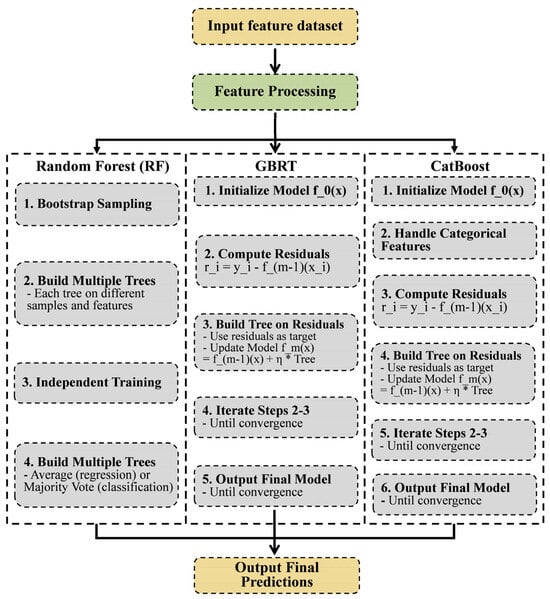
Figure 3. RF, GBRT and CatBoost predicted structures.

2.3.3. Determination of Model Parameters

Model parameters for the RF, GBRT, and CatBoost regression models were determined in a Python 3.7.10 environment based on model performance and stability. The dataset was randomly divided into training and test sets at a ratio of 7:3 prior to model training. All feature transformations, including the Box–Cox transformation and variable selection procedures, were performed using the training dataset only, and the optimized configurations were subsequently applied to the independent test dataset to assess predictive capability.

For the Random Forest (RF) model, the parameter configuration consisted of 800 decision trees (n_estimators = 800), square-root feature sampling (max_features = ‘sqrt’), and a fixed random seed (random_state = 0). The GBRT model was implemented using a gradient boosting framework, with key parameters such as tree depth, learning rate, and number of iterations adjusted to balance prediction accuracy and model complexity. The CatBoost model employed a mean absolute error (MAE) loss function, a tree depth of 7, and an iteration-based overfitting detection strategy. All models were evaluated using the same training–testing framework to ensure comparability among different regression algorithms.

2.3.4. Accuracy Metrics

Our analysis employs Mean Absolute Error (MAE) to evaluate the predictive accuracy of individual models and selects the optimal model for forecasting. The coefficient of determination (R²) is used to assess the closeness between the dataset and the fitted regression line, evaluating the predictive performance of the regression model. Root Mean Square Error (RMSE) is applied to measure the prediction error between the forecasted LAI values and the measured values.

MAE is a crucial metric for evaluating regression model prediction accuracy, measuring prediction error by calculating the average absolute difference between predicted and measured LAI values. This paper will output the MAE for each prediction model using Python 3.7 to select the optimal machine learning regression model.

$$MAE={\displaystyle \frac{1}{n}}{\displaystyle {\sum }_{i=1}^n|y_i-\widehat{y_i}|}$$

(1)

In the equation, n represents the number of samples in the training set; y_i denotes the measured LAI value of the i-th sample; $\widehat{y_i}$ is the predicted value of the i-th sample; $|y_i-\widehat{y_i}|$ indicates the absolute error between the measured value and the predicted LAI value for the i-th sample.

R² is a statistical metric used in regression analysis to assess the quality of model fit. It reflects the degree of alignment between observed and predicted values through regression relationships for RF, GBRT, and CatBoost models, thereby assessing the capability of each machine learning regression model to estimate LAI in mangrove forests, as shown in Equation (2).

$$R^2=1-{\displaystyle \frac{{{\displaystyle {\sum }_{i=1}^n(y_i-{\widehat{y}}_i)}}^2}{{{\displaystyle {\sum }_{i=1}^n(y_i-\overline{y})}}^2}}$$

(2)

In the equation, n is the number of samples; y_i is the actual value of the i-th sample; $\widehat{y_i}$ is the predicted value of the i-th sample; $\stackrel{\_}{y_i}$ is the mean of the measured LAI values; ${{\displaystyle {\sum }_{i=1}^n(y_i-{\widehat{y}}_i)}}^2$ is the residual sum of squares (RSS); ${{\displaystyle {\sum }_{i=1}^n(y_i-\overline{y})}}^2$ is the total sum of squares (TSS).

RMSE is primarily used to measure the discrepancy between predicted and actual values. It characterizes the degree of curve fit between predicted and measured values, serving as a metric for assessing the accuracy of model predictions, as shown in Equation (3).

$$RMSE=\sqrt{{\displaystyle \frac{1}{n}}{\displaystyle {\sum }_{i=1}^n{(y_i-{\widehat{y}}_i)}^2}}$$

(3)

In the equation, n is the number of samples; y_i is the actual value of the i-th sample; $\widehat{y_i}$ is the predicted value of the i-th sample; ${(y_i-{\widehat{y}}_i)}^2$ represents the squared error of the i-th sample.

3. Results

3.1. Dataset Statistical Characteristics and Sensitivity of LAI-Related Variables

To identify informative input variables for LAI modeling and to ensure the validity of subsequent regression analyses, normality tests and correlation analyses were conducted for both UAV and GF-6 datasets.

The results of the normality tests for the training and validation datasets indicate that both UAV and GF-6 data generally satisfy the normal distribution assumption, confirming that the datasets meet the statistical requirements for subsequent model construction (Figure 4a,d and Figure 5a,d).

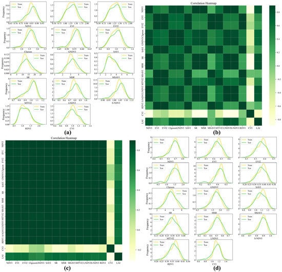
Figure 4. Normal distribution and heatmap of UAV and GF-6 data for Avicennia marina (AM). (a) UAV data normal distribution plot; (b) UAV data heatmap; (c) GF-6 data heatmap; (d) GF-6 data normal distribution plot.

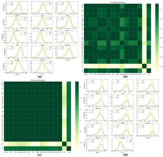
Figure 5. Normal distribution and heatmap of UAV and GF-6 data for Aegiceras corniculatum (AC). (a) UAV data normal distribution plot; (b) UAV data heatmap; (c) GF-6 data heatmap; (d) GF-6 data normal distribution plot.

Correlation analysis shows that vegetation indices for the AM tree species exhibit correlation coefficients (R) with LAI ranging from 0.70 to 0.78 (Table 3). Specifically, the MSR derived from UAV data shows the highest correlation with LAI (R = 0.782), whereas the SR derived from GF-6 data presents the strongest correlation among the satellite-based indices (R = 0.728). For the AC tree species, the correlation differences between UAV and GF-6 data are more pronounced. The UAV-derived LNDVI achieves the highest correlation with LAI (R = 0.838), while the GF-6-derived CIgreen shows the strongest correlation among the corresponding satellite indices (R = 0.732) (Figure 4b,c and Figure 5b,c). These correlation results provide a quantitative basis for identifying candidate variables for subsequent LAI modeling.

Table 3. Pearson correlation coefficients (R) between vegetation indices and measured LAI derived from UAV and GF-6 data for Avicennia marina (AM) and Aegiceras corniculatum (AC).

Vegetation Index	AM_UAV (R)	AM_GF-6 (R)	AC_UAV (R)	AC_GF-6 (R)
NDVI	0.762	0.688	0.825	0.678
EVI	0.376	0.715	0.669	0.712
EVI 2	0.299	0.703	0.616	0.718
CIgreen	0.649	0.596	0.782	0.732
GNDVI	0.646	0.580	0.785	0.717
SAVI	0.327	0.701	0.637	0.717
SR	0.774	0.728	0.776	0.707
MSR	0.782	0.715	0.821	0.700
MSAVI	0.100	0.692	0.260	0.714
MTVI2	0.428	0.725	0.680	0.713
LNDVI	0.777	0.706	0.838	0.692
S-NDVI	0.758	0.683	0.820	0.674
RDVI	0.173	0.703	0.415	0.717
CVI	−0.700	−0.307	−0.737	−0.038

Feature variable screening further reveals differences between UAV and GF-6 datasets across the two mangrove species. For UAV data, both AM and AC tree species retain NDVI, SR, MSR, LNDVI, S-NDVI, CVI, CIgreen, and GNDVI as core feature variables. In contrast, the selected feature variables derived from GF-6 data exhibit greater diversity. For the AM tree species, the retained indices include EVI, EVI2, SAVI, SR, MSR, MTVI2, LNDVI, and RDVI, while for the AC tree species, the selected features include EVI, EVI2, CIgreen, SAVI, SR, MSR, MSAVI, and MTVI2.

3.2. Effects of Box–Cox Transformation and Feature Importance Analysis

To improve data distribution characteristics and support subsequent regression analyses, Box–Cox transformations were applied to both the training and validation datasets for the UAV and GF-6 data.

The transformation results show that the normality of both datasets improved for the AM and AC tree species after Box–Cox transformation. For the AM species, the normality of the training and prediction datasets increased markedly following transformation (Figure 6a,b). For the AC species, the pronounced distribution discrepancy between the GF-6 training and validation datasets was substantially reduced after transformation (Figure 7a,b), indicating a more consistent data distribution between the two datasets.

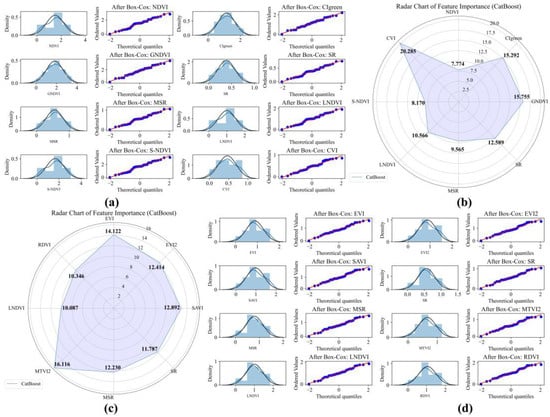
Figure 6. Box–Cox transformation and CatBoost feature variable selection of UAV and GF-6 data for Avicennia marina (AM). (a) UAV data Box–Cox transformation QQ plot; (b) UAV data feature variable selection chart; (c) GF-6 data feature variable selection chart; (d) GF-6 data Box–Cox transformation QQ plot.

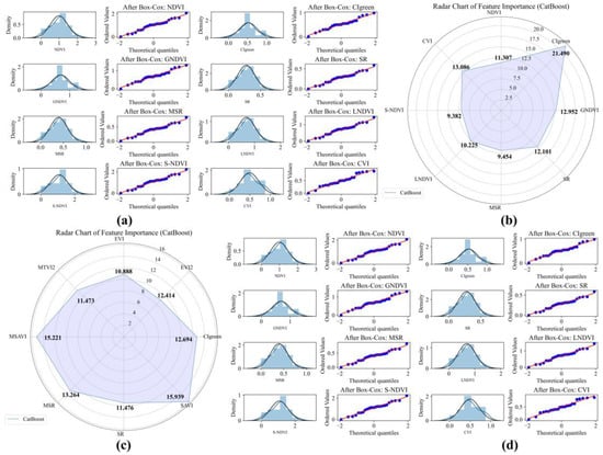
Figure 7. Box–Cox transformation and CatBoost feature variable selection of UAV and GF-6 data for Aegiceras corniculatum (AC). (a) UAV data Box–Cox transformation QQ plot; (b) UAV data feature variable selection chart; (c) GF-6 data feature variable selection chart; (d) GF-6 data Box–Cox transformation QQ plot.

Feature selection based on CatBoost feature importance rankings reveals distinct dominant variables across sensors and species. For the AM species, the most important feature derived from UAV data is CVI, with an importance score of 20.285, followed by GNDVI (15.755) and CIgreen (15.292). In contrast, for the GF-6 data, MTVI2 (16.116), EVI (14.122), and SAVI (12.892) exhibit the highest importance scores (Figure 6c,d).

For the AC species, feature importance patterns show similar sensor-dependent differences. In the UAV dataset, CIgreen, CVI, and GNDVI present the highest importance scores of 21.494, 13.086, and 12.952, respectively. For the GF-6 dataset, SAVI (15.939), MSAVI (15.221), and MSR (13.264) are identified as the most influential variables (Figure 7c,d).

3.3. Model Performance and Prediction Results for Mangrove Leaf Area Index

Three regression models—RF, CatBoost, and GBRT—were employed to estimate LAI for the training and validation datasets of AM and AC tree species. Model performance was evaluated using MAE, R², and RMSE metrics (Figure 8, Figure 9 and Figure 10). Clear differences in prediction accuracy were observed among data sources, regression models, and tree species.

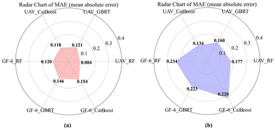
Figure 8. Model training results of UAV and GF-6 data. (a) Model training results of Avicennia marina (AM); (b) Model training results of Aegiceras corniculatum (AC).

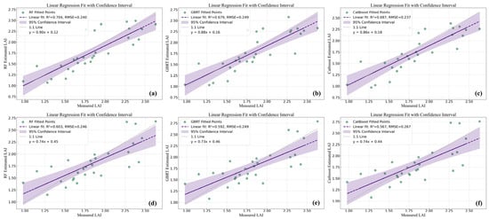
Figure 9. Prediction results of UAV and GF-6 data for Avicennia marina (AM). (a) RF regression model in UAV data; (b) GBRT regression model in UAV data; (c) CatBoost regression model in UAV data; (d) RF regression model in GF-6 data; (e) GBRT regression model in GF-6 data; (f) CatBoost regression model in GF-6 data.

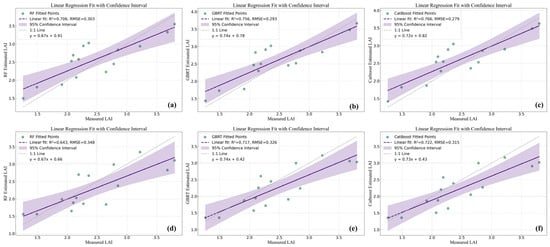
Figure 10. Prediction results of UAV and GF-6 data for Aegiceras corniculatum (AC). (a) RF regression model in UAV data; (b) GBRT regression model in UAV data; (c) CatBoost regression model in UAV data; (d) RF regression model in GF-6 data; (e) GBRT regression model in GF-6 data; (f) CatBoost regression model in GF-6 data.

Model training results based on MAE are presented in Figure 8. For both AM and AC tree species, MAE values derived from UAV data were consistently lower than those obtained from GF-6 data across all three models. In the AM species, RF achieved the lowest MAE among the three models for both UAV and GF-6 datasets, outperforming CatBoost and GBRT by 0.034 and 0.037, respectively, when using UAV data, and by 0.034 and 0.026, respectively, when using GF-6 data (Figure 8a). A similar pattern was observed for the AC species, where RF also yielded the lowest MAE values for both data sources, while CatBoost and GBRT exhibited higher training errors (Figure 8b).

For the AM tree species, prediction accuracy based on UAV data yielded R² values ranging from 0.679 to 0.704, with RMSE values between 0.240 and 0.249. Using GF-6 data, R² values ranged from 0.567 to 0.603, with RMSE values between 0.246 and 0.267. Among the three models, RF achieved the highest prediction accuracy for both data sources, with an R² value 0.025 higher and an RMSE value 0.009 lower than those of the GBRT model when using UAV data, and an R² value 0.036 higher and an RMSE value 0.021 lower than those of the CatBoost model when using GF-6 data (Table 4 and Figure 9).

Table 4. Model training and validation results for Avicennia marina (AM) and Aegiceras corniculatum (AC).

Evaluation Metrics	UAV_RF	UAV_GBRT	UAV_CatBoost	GF-6_RF	GF-6_GBRT	GF-6_CatBoost
AM_MAE	0.084	0.121	0.118	0.120	0.146	0.154
AM_R2	0.704	0.679	0.687	0.603	0.592	0.567
AM_RMSE	0.240	0.249	0.237	0.246	0.249	0.267
AC_MAE	0.177	0.160	0.134	0.234	0.223	0.220
AC_R2	0.706	0.756	0.766	0.643	0.717	0.722
AC_RMSE	0.303	0.293	0.279	0.348	0.326	0.315

For the AC tree species, prediction accuracy based on UAV data yielded R² values ranging from 0.706 to 0.766, with RMSE values between 0.279 and 0.303. Using GF-6 data, R² values ranged from 0.643 to 0.722, with RMSE values between 0.315 and 0.348. In this case, CatBoost achieved the highest prediction accuracy across both data sources. When applied to UAV data, CatBoost produced an R² value 0.060 higher than RF and 0.010 higher than GBRT, while reducing RMSE by 0.024 and 0.014, respectively. For GF-6 data, CatBoost also yielded the highest accuracy, with R² values 0.079 and 0.005 higher than those of RF and GBRT, and RMSE values 0.033 and 0.011 lower, respectively (Table 4, Figure 10).

3.4. LAI Retrieval and Spatial Distribution Patterns Across Mangrove Species

Although multi-index machine-learning models showed slightly better predictive performance during model evaluation, NDVI–LAI linear regression was adopted for spatial LAI mapping to enhance interpretability and spatial stability, and to reduce the risk of overfitting when extrapolating across the entire study area. LAI models for different mangrove species were constructed by integrating NDVI derived from UAV and GF-6 datasets with field-measured LAI data (Equations (4) and (5)). Species-specific NDVI–LAI linear relationships for AM and AC were established using UAV data. The AM model achieved an R² of 0.571 with an RMSE of 0.303, while the AC model yielded a higher R² of 0.637 and a lower RMSE of 0.247, with the associated 95% confidence intervals (CI) shown in Figure 11.

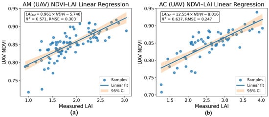
Figure 11. Species-specific NDVI–LAI linear relationships derived from UAV data for mangrove species. (a) NDVI–LAI relationship for Avicennia marina (AM); (b) NDVI–LAI relationship for Aegiceras corniculatum (AC).

Sampling points extracted from UAV imagery were used for model development, while independent in situ LAI measurements were used for validation. A random forest classifier combined with multi-scale segmentation was applied to classify mangroves in the UAV imagery into AM and AC species. The overall classification accuracy reached 87.39%, with a Kappa coefficient of 0.78 (Table 5 and Figure 12a).

Table 5. Accuracy assessment of UAV-based mangrove species classification for Avicennia marina (AM) and Aegiceras corniculatum (AC).

Species	Training Samples	Verification Samples	User’s Accuracy	Producer’s Accuracy	Kappa Coefficient	Overall Accuracy
AM	198	85	0.853	0.933	0.78	87.39%
AC	145	62	0.848	0.788

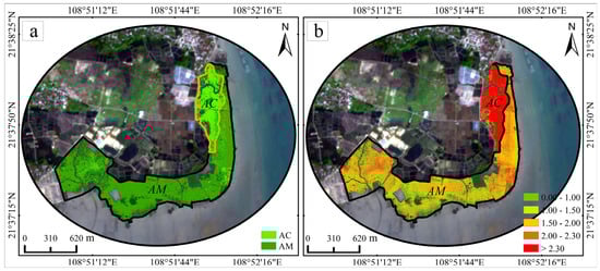
Figure 12. Classification and retrieval results of mangrove leaf area index for Avicennia marina (AM) and Aegiceras corniculatum (AC). (a) Classification results in UAV data; (b) Retrieval results in UAV data.

AM_UAV LAI-NDVI Model:

$$LA{I}_{AM\_UAV}=8.961\times NDVI-5.748$$

(4)

AC_UAV LAI-NDVI Model:

$$LA{I}_{AC\_UAV}=12.554\times NDVI-8.016$$

(5)

Based on the NDVI–LAI relationships for the two species and the corresponding classification results, species-level LAI spatial distribution maps were generated (Figure 12b), in which darker red indicates higher LAI values. According to in situ measurements, the mean LAI of AM was 1.87, while the mean LAI of AC was 2.60, yielding a difference of 0.73 (Table 1). In the LAI thematic maps, AM values were mainly distributed within the range of 1.5–2.0, whereas AC exhibited a higher proportion of pixels with LAI values exceeding 2.3 (Table 6). The mean LAI values derived from both mapped results and field measurements fell within the corresponding ranges for each species.

Table 6. Proportion of LAI value ranges for Avicennia marina (AM) and Aegiceras corniculatum (AC).

Species	LAI 0–1	LAI 1–1.5	LAI 1.5–2.0	LAI 2.0–2.3	LAI > 2.3
AM	14.64%	19.62%	42.02%	18.34%	5.38%
AC	3.33%	2.54%	4.42%	4.70%	85.01%

LAI thresholds were further used to classify mangrove health status, with LAI~0 representing dead mangroves, LAI~1 indicating poor condition, and LAI~2.3 representing healthy mangroves. Based on UAV-derived LAI data, the health status of different mangrove species was quantitatively assessed. For AM species, 14.64% of pixels exhibited LAI values between 0 and 1, 79.98% ranged from 1 to 2.3, and 5.38% exceeded 2.3. For AC species, 3.33% of pixels fell within 0 < LAI ≤ 1, 11.66% within 1 < LAI ≤ 2.3, and 85.01% exceeded 2.3 (Table 6). Accordingly, healthy mangroves (LAI > 1) accounted for 85.36% of the AM distribution, while unhealthy mangroves represented 14.64%. In contrast, healthy mangroves constituted 96.67% of the AC distribution, with only 3.33% classified as unhealthy.

Spatially, areas characterized by lower LAI values were primarily concentrated near localized disturbance zones. UAV orthoimages revealed low-LAI patches associated with wastewater discharge channels, Spartina alterniflora encroachment, and combined impacts of wastewater discharge and Spartina expansion. In contrast, areas distant from these disturbance sources generally exhibited higher LAI values.

4. Discussion

4.1. Spectral Index Sensitivity and Uncertainty in Leaf Area Index Retrieval

This study utilizes the optimal feature variables selected by CatBoost to establish curve-based relationships with measured LAI. Figure 13 shows the saturation patterns of LAI across different mangrove species in relation to variations in the optimal spectral indices. The results show that several commonly used indices, such as EVI, SAVI, and MSR, tend to exhibit saturation when LAI reaches approximately 2–3 or 3–4. In contrast, when LAI > 3, certain indices do not exhibit clear saturation but instead show a gradual increase or decrease, indicating relatively higher sensitivity under dense canopy conditions.

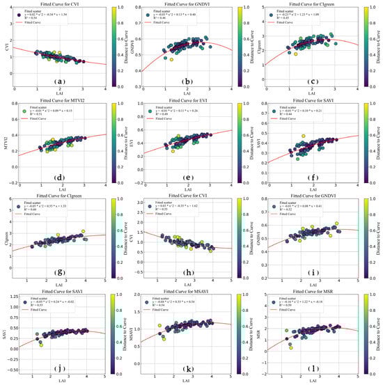
Figure 13. Sensitivity of optimal spectral indices to leaf area index (LAI). (a–c) Index sensitivity derived from UAV data for Avicennia marina (AM); (d–f) Index sensitivity derived from GF-6 data for Avicennia marina (AM); (g–i) Index sensitivity derived from UAV data for Aegiceras corniculatum (AC); (j–l) Index sensitivity derived from GF-6 data for Aegiceras corniculatum (AC).

To further analyze the sensitivity of optimal feature variables for AM and AC species, the selected indices mainly include two-band indices composed of red and near-infrared bands (e.g., SAVI, MSAVI, EVI, and MSR), near-infrared and green bands (e.g., GNDVI and CIgreen), as well as three-band indices composed of near-infrared, red, and green bands (e.g., CVI and MTVI2). The wavelength ranges of these LAI-sensitive indices span approximately 450–900 nm, which is consistent with the findings of Zhao (2023), who reported effective LAI-sensitive wavelengths ranging from 443 to 908 nm [11].

Different spectral bands exhibit varying sensitivities to LAI, leading to distinct saturation characteristics among vegetation indices. When LAI < 3, the red and blue bands generally show higher sensitivity to changes in LAI. Although the green band may exhibit lower sensitivity than the red and blue bands under certain conditions, it demonstrates a broader dynamic range in response to LAI variations [57]. Three-band indices such as CVI and MTVI2, which integrate near-infrared, red, and green bands, and two-band indices such as CIgreen, composed of near-infrared and green bands, maintain sensitivity under higher LAI conditions. In contrast, indices such as MSR and MSAVI tend to approach saturation as LAI increases (Figure 13). These results indicate that different spectral band combinations emphasize different aspects of canopy structure and density.

Beyond index formulation, sensor-related characteristics may also influence the sensitivity of vegetation indices to LAI. Differences in spatial resolution affect the degree to which canopy heterogeneity and fine-scale structural variations can be captured, particularly under structurally complex canopies [58,59]. Variations in spectral resolution and band configuration further influence index responsiveness to canopy density and chlorophyll content, especially for indices constructed from red, green, and near-infrared bands [41,44].

In addition, radiometric resolution and calibration accuracy can affect the stability and precision of reflectance measurements, thereby influencing vegetation index performance and inter-sensor comparability [37,60]. Consequently, differences in LAI sensitivity among vegetation indices may reflect the combined effects of index formulation and sensor characteristics rather than band selection alone [61].

Furthermore, variability in field-measured LAI may also contribute to uncertainty in sensitivity analysis. Previous studies have shown that canopy LAI measurements are influenced by sampling strategy, canopy heterogeneity, and short-term environmental conditions, which may introduce variability even within the same vegetation type [62]. This measurement variability, together with differences in sensor resolution, underscores the importance of constructing and evaluating diverse spectral indices to improve the robustness and reliability of LAI retrieval across mangrove species and environmental conditions. Model performance metrics (R², RMSE, and MAE) reported in this study represent average evaluation results under a given training–validation partition and may vary with different sample splits. In addition, differences in sensor resolution and canopy spatial heterogeneity may introduce uncertainty into LAI sensitivity analysis, which should be considered when interpreting index performance.

4.2. Effects of Regression Model Selection on Leaf Area Index Retrieval

To identify the most suitable LAI retrieval model, this study compares the performance of three machine learning regression algorithms, namely random forest (RF), gradient boosting regression tree (GBRT), and CatBoost. Differences in model performance across mangrove species and data sources reflect variations in algorithm structure, robustness to noise, and sensitivity to feature interactions.

RF and CatBoost generally exhibit higher robustness under different environmental conditions, highlighting their suitability for LAI inversion tasks [63]. RF has been shown to perform well when training sample sizes are relatively limited, owing to its ensemble structure and the independence of individual decision trees, which reduces sensitivity to noisy predictor variables [24,64]. This characteristic is particularly advantageous for vegetation LAI estimation, where environmental noise and measurement uncertainty are often present. In contrast, GBRT may be more sensitive to noise accumulation during sequential tree construction, which can reduce predictive stability under complex environmental conditions [53].

CatBoost represents an optimization of traditional gradient boosting algorithms and demonstrates advantages in handling feature interactions and suppressing over-fitting, particularly under conditions where input variables exhibit complex nonlinear relationships [65,66]. These properties may explain its improved adaptability for certain mangrove species, where canopy structure and spectral responses are more heterogeneous. As a result, CatBoost can outperform RF under identical inputs when estimation uncertainty increases.

Although RF and CatBoost exhibit different strengths, the differences in predictive performance between these two models remain relatively small, indicating that both algorithms are capable of effectively capturing the nonlinear relationships between spectral variables and LAI. This observation is consistent with previous comparative studies showing that ensemble learning approaches often yield comparable accuracy in vegetation parameter inversion when appropriately configured [31]. Consequently, evaluating multiple regression models provides a robust basis for selecting suitable algorithms and reducing uncertainty in LAI estimation, thereby improving the reliability of mangrove canopy analysis [16].

4.3. Relationship Between Leaf Area Index and Mangrove Health Status

Leaf area index (LAI) is widely recognized as a key indicator of canopy structure and photosynthetic capacity and is commonly used as a proxy for assessing mangrove condition and relative health status. Previous studies have suggested indicative LAI thresholds to distinguish broad canopy conditions, such as dead or severely degraded stands (LAI~0), poorly developed canopies (LAI~1), and well-developed or healthy canopies (LAI ≥ 2.3), while acknowledging that these thresholds are not absolute and may vary across species, environments, and measurement methods [16,67,68].

Based on UAV-derived LAI estimates, this study quantitatively characterized the canopy condition of different mangrove species. For AM, 14.64% of the area exhibited LAI values between 0 and 1, 79.98% ranged between 1 and 2.3, and 5.38% exceeded 2.3. In contrast, AC showed a markedly different distribution, with 3.33% of the area having LAI ≤ 1, 11.66% between 1 and 2.3, and 85.01% exceeding 2.3 (Table 6; Figure 14). When applying these indicative thresholds, canopies classified as relatively healthy (LAI > 1) accounted for 85.36% of AM stands and 96.67% of AC stands.

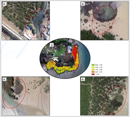
Figure 14. Spatial patterns of mangrove LAI and associated local conditions. (a) LAI inversion results derived from UAV data, with subpanels (a₁–a₄) highlighting representative areas exposed to potential risks; (a₁) mangrove area potentially affected by aquaculture wastewater discharge; (a₂–a₄) mangrove areas potentially impacted by Spartina alterniflora invasion.

The observed differences in LAI distribution suggest that AC generally exhibits denser and more developed canopies than AM within the study area, which is consistent with previous findings reporting interspecific differences in mangrove canopy structure under comparable environmental settings [16,68]. However, it should be noted that LAI-based health classification is sensitive to threshold selection and measurement uncertainty. Variability in LAI estimates may arise from species-specific canopy architecture, sub-canopy heterogeneity, seasonal phenology, and uncertainties associated with both field measurements and remote sensing retrieval.

Spatial analysis further revealed that areas exhibiting lower LAI values tend to co-occur with localized environmental disturbances, including proximity to wastewater discharge channels and the presence of Spartina alterniflora encroachment (Figure 14a₁–a₄). Rather than implying direct causality, these spatial associations indicate that such stressors may contribute to canopy degradation or reduced growth vigor under certain conditions. Similar patterns linking reduced LAI to anthropogenic disturbance, invasive species, or altered hydrological regimes have been reported in other mangrove and coastal wetland studies [67,69,70,71].

Overall, the results indicate that mangroves in the SJ region are generally in good condition, although localized areas exhibit reduced canopy development. LAI-based spatial patterns therefore provide an effective means of identifying relative canopy condition and potential stress hotspots, offering valuable support for mangrove monitoring, management, and ecological restoration. It should also be mentioned that the area proportions of LAI-based health classes are influenced by LAI estimation uncertainty, classification thresholds, and the intrinsic spatial heterogeneity of mangrove canopies. Therefore, the reported health class distributions are intended to reflect relative spatial patterns rather than exact quantitative proportions. It should be noted that the LAI-based health thresholds and model configurations proposed in this study are calibrated specifically for the SJ mangrove site in the Beibu Gulf and for the two dominant mangrove species considered (Avicennia marina and Aegiceras corniculatum). Their transferability to other regions or mangrove species may be influenced by differences in environmental conditions, canopy structure, and sensor characteristics, and therefore should be approached with appropriate caution.

5. Conclusions

As an important indicator of mangrove ecosystem condition, leaf area index (LAI) is closely related to canopy structure and vegetation vigor. This study investigated the sensitivity of multispectral vegetation indices to LAI and developed optimal LAI retrieval models for Avicennia marina (AM) and Aegiceras corniculatum (AC) using UAV and GF-6 data. Spatial LAI distribution was utilized to support the assessment of mangrove condition and potential health risks.

The results indicate that CVI and CIgreen are the most sensitive vegetation indices for AM and AC species in UAV data, respectively, while MTVI 2 and SAVI show the highest sensitivity for GF-6 imagery. The optimal machine learning regression model for AM species is random forest (RF), whereas CatBoost performs best for AC species. Both UAV and GF-6 data demonstrate strong capability for mangrove LAI estimation, with UAV data achieving higher retrieval accuracy. LAI values do not exhibit saturation when LAI exceeds 3 and instead increase gradually with increasing values of vegetation indices such as CVI, MTVI 2, and CIgreen.

Based on the spatial distribution of LAI derived from UAV data, the study area’s mangroves generally exhibit favorable growth conditions, while localized areas with relatively low LAI values suggest potential stress. Wastewater discharge from aquaculture ponds and the ongoing expansion of Spartina alterniflora may be contributing factors affecting mangrove growth in the SJ region. Monitoring LAI holds significant importance for mangrove ecosystem health. When interpreted with appropriate caution and uncertainty awareness, LAI thresholds can offer early-warning insights.

Overall, this study demonstrates the effectiveness of integrating UAV and satellite remote sensing data with machine learning algorithms for mangrove LAI monitoring and early-stage ecosystem assessment. Future work will focus on expanding LAI field measurements and incorporating multi-temporal UAV and satellite data across the Beibu Gulf region, providing stronger data support for mangrove conservation, management, and restoration decision-making.

References

- Lymburner, L.; Bunting, P.; Lucas, R.; Scarth, P.; Alam, I.; Phillips, C.; Ticehurst, C.; Held, A. Mapping the multi-decadal mangrove dynamics of the Australian coastline. Remote Sens. Environ. 2020, 238, 111185. [Google Scholar] [CrossRef]
- Li, Q.; Wong, F.K.K.; Fung, T.; Nichol, J.; Wong, M.S. Mapping multi-layered mangroves from multispectral, hyperspectral, and LiDAR data. Remote Sens. Environ. 2021, 258, 112403. [Google Scholar] [CrossRef]
- Wang, D.; Wan, B.; Liu, J.; Su, Y.; Guo, Q.; Qiu, P.; Wu, X. Estimating aboveground biomass of the mangrove forests on northeast Hainan Island in China using an upscaling method from field plots, UAV-LiDAR data and Sentinel-2 imagery. Int. J. Appl. Earth Obs. Geoinf. 2020, 85, 101986. [Google Scholar] [CrossRef]
- Ward, R.D.; Friess, D.A.; Day, R.H.; MacKenzie, R.A. Impacts of climate change on mangrove ecosystems: A region-by-region overview. Ecosyst. Health Sustain. 2016, 2, e01211. [Google Scholar] [CrossRef]
- Xie, Q.; Dash, J.; Huete, A.; Jiang, A.; Yin, G.; Ding, Y.; Peng, D.; Qin, Q.; Mortimer, H.; Casa, R.; et al. Retrieval of crop biophysical parameters from Sentinel-2 remote sensing imagery. Int. J. Appl. Earth Obs. Geoinf. 2019, 80, 187–195. [Google Scholar] [CrossRef]
- Almeida, L.T.; Olímpio, J.L.S.; Pantalena, A.F.; Almeida, B.S.; Soares, M.O. Evaluating ten years of management effectiveness in a mangrove protected area. Ocean Coast. Manag. 2016, 125, 29–37. [Google Scholar] [CrossRef]
- Fu, B.; Sun, J.; Wang, Y.; Chen, B.; Yang, Z.; Zhang, B.; Zhang, L. Evaluation of LAI estimation of mangrove communities using DLR and ELR algorithms with UAV, hyperspectral, and SAR images. Front. Mar. Sci. 2022, 9, 944454. [Google Scholar] [CrossRef]
- Zhang, X.; Song, P. Estimating urban evapotranspiration at 10 m resolution using vegetation information from Sentinel-2: A case study for the Beijing Sponge City. Remote Sens. 2021, 13, 2048. [Google Scholar] [CrossRef]
- Binh, N.A.; Hauser, L.T.; Hoa, P.V.; Thao, G.T.P.; An, N.N.; Nhut, H.S.; Phuong, T.A.; Verrelst, J. Quantifying mangrove leaf area index from Sentinel-2 imagery using hybrid models and active learning. Int. J. Remote Sens. 2022, 43, 5636–5657. [Google Scholar] [CrossRef]
- Zhang, Y.; Yang, J.; Du, L. Analyzing the effects of hyperspectral ZhuHai-1 band combinations on LAI estimation based on the PROSAIL model. Sensors 2021, 21, 1869. [Google Scholar] [CrossRef]
- Zhao, D.; Zhen, J.; Zhang, Y.; Wang, L.; Gao, J.; Liu, M.; Zhang, C. Mapping mangrove leaf area index (LAI) by combining remote sensing images with PROSAIL-D and XGBoost methods. Remote Sens. Ecol. Conserv. 2023, 9, 315. [Google Scholar] [CrossRef]
- Li, Q.; Wong, F.K.K.; Fung, T.; Brown, L.A.; Dash, J. Assessment of active LiDAR data and passive optical imagery for double-layered mangrove leaf area index estimation: A case study in Mai Po, Hong Kong. Remote Sens. 2023, 15, 2551. [Google Scholar] [CrossRef]
- Tian, J.; Wang, L.; Li, X.; Gong, H.; Shi, C.; Zhong, R.; Liu, X. Comparison of UAV and WorldView-2 imagery for mapping leaf area index of mangrove forest. Int. J. Appl. Earth Obs. Geoinf. 2017, 61, 22–31. [Google Scholar] [CrossRef]
- DiGiacomo, A.E.; Giannelli, R.; Puckett, B.; Smith, E.; Ridge, J.T.; Davis, J. Considerations and tradeoffs of UAS-based coastal wetland monitoring in the southeastern United States. Front. Remote Sens. 2022, 3, 924969. [Google Scholar] [CrossRef]
- Deng, L.; Chen, B.; Yan, M.; Fu, B.; Yang, Z.; Zhang, B.; Zhang, L. Estimation of species-scale canopy chlorophyll content in mangroves from UAV and GF-6 data. Forests 2023, 14, 1417. [Google Scholar] [CrossRef]
- Zhu, Y.; Liu, K.; Liu, L.; Myint, S.W.; Wang, S.; Liu, H.; He, Z. Exploring the potential of WorldView-2 red-edge band-based vegetation indices for estimation of mangrove leaf area index with machine learning algorithms. Remote Sens. 2017, 9, 1060. [Google Scholar] [CrossRef]
- Heenkenda, M.K.; Joyce, K.E.; Maier, S.W.; de Bruin, S. Quantifying mangrove chlorophyll from high spatial resolution imagery. ISPRS J. Photogramm. Remote Sens. 2015, 108, 234–244. [Google Scholar] [CrossRef]
- Green, E.P.; Mumby, P.J.; Edwards, A.J.; Clark, C.D.; Ellis, A.C. Estimating leaf area index of mangroves from satellite data. Aquat. Bot. 1997, 58, 11–19. [Google Scholar] [CrossRef]
- Guo, X.; Wang, M.; Jia, M.; Wang, W. Estimating mangrove leaf area index based on red-edge vegetation indices: A comparison among UAV, WorldView-2 and Sentinel-2 imagery. Int. J. Appl. Earth Obs. Geoinf. 2021, 103, 102493. [Google Scholar] [CrossRef]
- Tran, T.V.; Reef, R.; Zhu, X. A review of spectral indices for mangrove remote sensing. Remote Sens. 2022, 14, 4868. [Google Scholar] [CrossRef]
- Manna, S.; Raychaudhuri, B. Retrieval of leaf area index and stress conditions for Sundarban mangroves using Sentinel-2 data. Int. J. Remote Sens. 2020, 41, 1019–1039. [Google Scholar] [CrossRef]
- Zhen, J.; Jiang, X.; Xu, Y.; Miao, J.; Zhao, D.; Wang, J.; Wang, J.; Wu, G. Mapping leaf chlorophyll content of mangrove forests with Sentinel-2 images of four periods. Int. J. Appl. Earth Obs. Geoinf. 2021, 102, 102387. [Google Scholar] [CrossRef]
- Juniansah, A.; Tama, G.C.; Febriani, K.R.; Baharain, M.N.; Kanekaputra, T.; Wulandari, Y.S.; Kamal, M. Mangrove leaf area index estimation using Sentinel-2A imagery in Teluk Ratai, Pesawaran Lampung. IOP Conf. Ser. Earth Environ. Sci. 2018, 165, 012004. [Google Scholar] [CrossRef]
- Li, Q. Mangrove Species Classification and Leaf Area Index Estimation from Multispectral, Hyperspectral and LiDAR Data in Mai Po Nature Reserve, Hong Kong. Ph.D. Thesis, The Chinese University of Hong Kong, Hong Kong, China, 2020. [Google Scholar]
- Pipia, L.; Amin, E.; Belda, S.; Salinero-Delgado, M.; Verrelst, J. Green LAI mapping and cloud gap-filling using Gaussian process regression in Google Earth Engine. Remote Sens. 2021, 13, 403. [Google Scholar] [CrossRef] [PubMed]
- Prasad, R.; Pandey, A.; Singh, K.P.; Singh, V.; Mishra, R.; Singh, D. Retrieval of spinach crop parameters by microwave remote sensing with back propagation artificial neural networks: A comparison of different transfer functions. Adv. Space Res. 2012, 50, 363–370. [Google Scholar] [CrossRef]
- Walthall, C.; Dulaney, W.; Anderson, M.; Gallo, K. A comparison of empirical and neural network approaches for estimating corn and soybean leaf area index from Landsat ETM+ imagery. Remote Sens. Environ. 2004, 92, 465–474. [Google Scholar] [CrossRef]
- Lou, P.; Fu, B.; He, H.; Chen, J.; Wu, T.; Lin, X.; Liu, L.; Fan, D.; Deng, T. An effective method for canopy chlorophyll content estimation of marsh vegetation based on multiscale remote sensing data. IEEE J. Sel. Top. Appl. Earth Obs. Remote Sens. 2021, 14, 5311–5325. [Google Scholar] [CrossRef]
- Miao, J.; Zhen, J.; Wang, J.; Zhao, D.; Jiang, X.; Shen, Z.; Gao, C.; Wu, G. Mapping seasonal leaf nutrients of mangrove with Sentinel-2 images and XGBoost method. Remote Sens. 2022, 14, 3679. [Google Scholar] [CrossRef]
- Hancock, J.T.; Khoshgoftaar, T.M. CatBoost for big data: An interdisciplinary review. J. Big Data 2020, 7, 94. [Google Scholar] [CrossRef]
- Luo, M.; Wang, Y.; He, Y.; Li, X. Combination of feature selection and CatBoost for prediction: The first application to the estimation of aboveground biomass. Forests 2021, 12, 216. [Google Scholar] [CrossRef]
- Bunt, J.S.; Boto, K.G.; Boto, G. A survey method for estimating potential levels of mangrove forest primary production. Mar. Biol. 1979, 52, 123–128. [Google Scholar] [CrossRef]
- Tucker, C.J. Red and photographic infrared linear combinations for monitoring vegetation. Remote Sens. Environ. 1979, 8, 127–150. [Google Scholar] [CrossRef]
- Gitelson, A.A.; Kaufman, Y.J.; Merzlyak, M.N. Use of a green channel in remote sensing of global vegetation from EOS-MODIS. Remote Sens. Environ. 1996, 58, 289–298. [Google Scholar] [CrossRef]
- Jiang, Z.; Huete, A.R. Linearization of NDVI based on its relationship with vegetation fraction. Photogramm. Eng. Remote Sens. 2010, 76, 965–975. [Google Scholar] [CrossRef]
- Liu, F.; Qin, Q.; Zhan, Z. A novel dynamic stretching solution to eliminate saturation effect in NDVI and its application in drought monitoring. Chin. Geogr. Sci. 2012, 22, 683–694. [Google Scholar] [CrossRef]
- Huete, A.; Didan, K.; Miura, T.; Rodriguez, E.P.; Gao, X.; Ferreira, L.G. Overview of the radiometric and biophysical performance of the MODIS vegetation indices. Remote Sens. Environ. 2002, 83, 195–213. [Google Scholar]
- Jiang, Z.; Huete, A.R.; Didan, K.; Miura, T. Development of a two-band enhanced vegetation index without a blue band. Remote Sens. Environ. 2008, 112, 3833–3845. [Google Scholar] [CrossRef]
- Jain, N.; Ray, S.S.; Singh, J.P.; Sharma, R.; Panigrahy, S. Use of hyperspectral data to assess the effects of different nitrogen applications on a potato crop. Precis. Agric. 2007, 8, 225–239. [Google Scholar] [CrossRef]
- Jordan, C.F. Derivation of leaf-area index from quality of light on the forest floor. Ecology 1969, 50, 663–666. [Google Scholar] [CrossRef]
- Haboudane, D.; Miller, J.R.; Pattey, E.; Zarco-Tejada, P.J.; Strachan, I.B. Hyperspectral vegetation indices and novel algorithms for predicting green LAI of crop canopies: Modeling and validation in the context of precision agriculture. Remote Sens. Environ. 2004, 90, 337–352. [Google Scholar] [CrossRef]
- Chen, J.M. Evaluation of vegetation indices and a modified simple ratio for boreal applications. Can. J. Remote Sens. 1996, 22, 229–242. [Google Scholar] [CrossRef]
- Gitelson, A.A.; Gritz, Y.; Merzlyak, M.N. Relationships between leaf chlorophyll content and spectral reflectance and algorithms for non-destructive chlorophyll assessment in higher plant leaves. J. Plant Physiol. 2003, 160, 271–282. [Google Scholar] [CrossRef]
- Gitelson, A.A.; Keydan, G.P.; Merzlyak, M.N. Three-band model for noninvasive estimation of chlorophyll, carotenoids, and anthocyanin contents in higher plant leaves. Geophys. Res. Lett. 2006, 33, L11402. [Google Scholar] [CrossRef]
- Vincini, M.; Frazzi, E.; D’Alessio, P. Comparison of Narrow-Band and Broad-Band Vegetation Indices for Canopy Chlorophyll Density Estimation in Sugar Beet; Precision Agriculture ’07; Wageningen Academic Publishers: Wageningen, The Netherlands, 2007; pp. 189–196. [Google Scholar]
- Vincini, M.; Frazzi, E.; D’Alessio, P. A broad-band leaf chlorophyll vegetation index at the canopy scale. Precis. Agric. 2008, 9, 303–319. [Google Scholar] [CrossRef]
- Qi, J.; Chehbouni, A.; Huete, A.R.; Kerr, Y.H.; Sorooshian, S. A modified soil adjusted vegetation index. Remote Sens. Environ. 1994, 48, 119–126. [Google Scholar] [CrossRef]
- Roujean, J.L.; Breon, F.M. Estimating PAR absorbed by vegetation from bidirectional reflectance measurements. Remote Sens. Environ. 1995, 51, 375–384. [Google Scholar] [CrossRef]
- Huete, A.R. A soil-adjusted vegetation index (SAVI). Remote Sens. Environ. 1988, 25, 295–309. [Google Scholar] [CrossRef]
- Quinlan, J.R. Induction of decision trees. Mach. Learn. 1986, 1, 81–106. [Google Scholar] [CrossRef]
- Loh, W.Y. Classification and regression trees. Wiley Interdiscip. Rev. Data Min. Knowl. Discov. 2011, 1, 14–23. [Google Scholar] [CrossRef]
- Johansson, U.; Boström, H.; Löfström, T.; Carlsson, L.; Gunnarsson, E.; Jonsson, P.; Bäckström, A.; Gustafsson, M. Regression conformal prediction with random forests. Mach. Learn. 2014, 97, 155–176. [Google Scholar] [CrossRef]
- Friedman, J.H. Greedy function approximation: A gradient boosting machine. Ann. Stat. 2001, 29, 1189–1232. [Google Scholar] [CrossRef]
- Wang, L.; Zhang, Y.; Yao, Y.; Li, X.; Chen, H.; Zhou, Q.; Liu, Y. GBRT-based estimation of terrestrial latent heat flux in the Haihe River Basin from satellite and reanalysis datasets. Remote Sens. 2021, 13, 1054. [Google Scholar] [CrossRef]
- Dorogush, A.V.; Ershov, V.; Gulin, A. CatBoost: Gradient boosting with categorical features support. arXiv 2018, arXiv:1810.11363. [Google Scholar] [CrossRef]
- Dorogush, A.V.; Gulin, A.; Gusev, G.; Ershov, V.; Prokhorenkova, L. Fighting biases with dynamic boosting. arXiv 2017, arXiv:1706.09516. [Google Scholar]
- Wang, F.; Huang, J.; Tang, Y.-L.; Wang, X.-Z. New vegetation index and its application in estimating leaf area index of rice. Rice Sci. 2007, 14, 195–203. [Google Scholar] [CrossRef]
- Turner, D.P.; Cohen, W.B.; Kennedy, R.E.; Fassnacht, K.S.; Briggs, J.M. Relation-ships between leaf area index and Landsat TM spectral vegetation indices across three temperate zone sites. Remote Sens. Environ. 1999, 70, 52–68. [Google Scholar] [CrossRef]
- Garrigues, S.; Allard, D.; Baret, F.; Weiss, M. Influence of landscape spatial heterogeneity on the non-linear estimation of leaf area index from moderate spatial resolution remote sensing data. Remote Sens. Environ. 2008, 105, 286–298. [Google Scholar] [CrossRef]
- Schowengerdt, R.A. Remote Sensing: Models and Methods for Image Processing, 3rd ed.; Academic Press: Amsterdam, The Netherlands, 2007. [Google Scholar]
- Weiss, M.; Baret, F.; Myneni, R.B.; Pragnère, A.; Knyazikhin, Y. Investigation of a model inversion technique to estimate canopy biophysical variables from spectral and directional reflectance data. Agronomie 2004, 20, 3–22. [Google Scholar] [CrossRef]
- Jonckheere, I.; Fleck, S.; Nackaerts, K.; Muys, B.; Coppin, P.; Weiss, M.; Baret, F. Review of methods for in situ leaf area index determination: Part I. Theories, sensors and hemispherical photography. Agric. For. Meteorol. 2004, 121, 19–35. [Google Scholar] [CrossRef]
- Breiman, L. Random forests. Mach. Learn. 2001, 45, 5–32. [Google Scholar] [CrossRef]
- Montorio, R.; Pérez-Cabello, F.; Alves, D.B.; García-Martín, A. Unitemporal approach to fire severity mapping using multi-spectral synthetic databases and Random Forests. Remote Sens. Environ. 2020, 249, 112025. [Google Scholar] [CrossRef]
- Cracknell, M.J.; Reading, A.M. Geological mapping using remote sensing data: A comparison of five machine learning algorithms, their response to variations in the spatial distribution of training data and the use of explicit spatial information. Comput. Geosci. 2014, 63, 22–33. [Google Scholar] [CrossRef]
- Zhang, Y.; Zhao, Z.; Zheng, J. CatBoost: A new approach for estimating daily reference crop evapotranspiration in arid and semi-arid regions of Northern China. J. Hydrol. 2020, 588, 125087. [Google Scholar] [CrossRef]
- Lovelock, C.E.; Feller, I.C.; McKee, K.L.; Engelbrecht, B.M.J.; Ball, M.C. The effect of nutrient enrichment on growth, photosynthesis and hydraulic conductance of dwarf mangroves in Panama. Funct. Ecol. 2004, 18, 25–33. [Google Scholar] [CrossRef]
- Asner, G.P.; Scurlock, J.M.O.; Hicke, J.A. Global synthesis of leaf area index observations: Implications for ecological and remote sensing studies. Glob. Ecol. Biogeogr. 2003, 12, 191–205. [Google Scholar] [CrossRef]
- Alongi, D.M. Mangrove forests: Resilience, protection from tsunamis, and responses to global climate change. Estuar. Coast. Shelf Sci. 2008, 76, 1–13. [Google Scholar] [CrossRef]
- Friess, D.A.; Webb, E.L. Variability in mangrove change estimates and implications for the assessment of ecosystem service provision. Glob. Ecol. Biogeogr. 2014, 23, 715–725. [Google Scholar] [CrossRef]
- Xie, X.F.; Sun, X.M.; Wu, T.; Jiang, G.J.; Pu, L.J.; Xiang, Q. Impacts of Spartina alterniflora invasion on coastal wetland ecosystem: Advances and prospects. Ying Yong Sheng Tai Xue Bao. (J. Appl. Ecol.) 2020, 31, 2119–2128. [Google Scholar]
Disclaimer/Publisher’s Note: The statements, opinions and data contained in all publications are solely those of the individual author(s) and contributor(s) and not of MDPI and/or the editor(s). MDPI and/or the editor(s) disclaim responsibility for any injury to people or property resulting from any ideas, methods, instructions or products referred to in the content. |
© 2026 by the authors. Licensee MDPI, Basel, Switzerland. This article is an open access article distributed under the terms and conditions of the Creative Commons Attribution (CC BY) license.