Abstract
Forestry environments—such as logging sites, transport trails, and resource monitoring areas—are characterized by rugged terrain and irregularly distributed obstacles, which pose substantial challenges for AGV route planning. This poses challenges for route planning in automated guided vehicles (AGVs) and forestry machinery. To address these challenges, this study proposes a hybrid path optimization method that integrates an improved A* algorithm with the Dynamic Window Approach (DWA). At the global planning level, the improved A* incorporates a dynamically weighted heuristic function, a steering-penalty term, and Floyd-based path smoothing to enhance path feasibility and continuity. In terms of local planning, the improved DWA algorithm employs adaptive weight adjustment, risk-perception factors, a sub-goal guidance mechanism, and a non-uniform and adaptive sampling strategy, thereby strengthening obstacle avoidance in dynamic environments. Simulation experiments on two-dimensional grid maps demonstrate that this method reduces path lengths by an average of 6.82%, 8.13%, and 21.78% for 20 × 20, 30 × 30, and 100 × 100 maps, respectively; planning time was reduced by an average of 21.02%, 16.65%, and 9.33%; total steering angle was reduced by an average of 100°, 487.5°, and 587.5°. These results indicate that the proposed hybrid algorithm offers practical technical guidance for intelligent forestry operations in complex natural environments, including timber harvesting, biomass transportation, and precision stand management.
1. Introduction
In recent years, the development of intelligent forestry has driven increasing demand for autonomous equipment capable of operating under complex natural conditions. Forestry Automated Guided Vehicles (F-AGVs) are being deployed for transporting timber, collecting biomass, and monitoring forest resources. Compared with indoor or factory environments, forest terrains present challenges such as uneven ground, soft soil, and irregularly distributed trees, which cause slippage and motion uncertainty [1]. Consequently, path-planning algorithms designed for structured environments must be adapted to ensure real-time obstacle avoidance and path smoothness in forestry applications. To address these needs, this paper focuses on improving AGV navigation performance in simulated forest environments, aiming to provide theoretical and technical references for the automation and digitization of forestry operations.
In addition, forestry operations impose even more stringent demands on autonomous mobile equipment. Forest environments typically feature rugged terrain, diverse obstacle types, irregular distributions, and significant dynamic changes, making path planning and obstacle avoidance particularly challenging. In recent years, researchers have begun exploring the application of intelligent navigation and control methods to forestry equipment. For instance, one study proposed an autonomous driving control system for forestry forwarders based on Global Navigation Satellite System/Inertial Navigation System (GNSS/INS) to enhance the autonomous driving and path-following capabilities of forestry machinery. However, its obstacle avoidance performance in complex dynamic environments still requires optimization [2]. Concurrently, mobile laser scanning and Simultaneous Localization and Mapping (SLAM) technologies have gained widespread adoption in forest resource inventories, providing crucial means for mobile robots to construct environmental maps and perceive forest spatial structures. Nevertheless, achieving efficient path planning and dynamic obstacle avoidance based on these technologies remains a significant challenge [3]. These studies indicate that forestry robots and AGVs similarly require efficient and robust path planning and control methods within forest environments.
For path-planning problems, traditional methods such as A* and Dijkstra are widely adopted due to their simplicity and ease of implementation. However, in complex environments, they often suffer from low search efficiency, redundant path nodes, and frequent abrupt turns [4,5,6]. Taking the A* algorithm as an example, the paths it generates frequently hug obstacles, posing collision risks, and it struggles to handle sudden obstacles in dynamic environments. These shortcomings are particularly pronounced in forest environments and industrial settings with high-frequency scheduling. To enhance algorithmic performance, researchers have proposed various A* improvements, One of the more mainstream approaches in A* is to design an adaptive evaluation function, which allows the algorithm to adapt to the environment, thereby improving search speed and flexibility [7], including optimizing cost functions and heuristics to improve path smoothness and environmental adaptability [8,9,10], as well as reducing search nodes through diagonal octant neighborhood expansion and integrating A* with artificial potential fields [11,12].
Meanwhile, the Dynamic Window Approach (DWA) has emerged as a key method for local path planning due to its excellent real-time performance and obstacle avoidance capabilities. Related research has primarily focused on optimizing evaluation functions and improving sampling strategies to enhance its environmental adaptability and robustness [13,14]; Kim and Yang [15] optimized DWA using reinforcement learning to achieve higher real-time performance in dynamic environments; Cao et al. [16] proposed a path-planning method for mobile robots based on a smooth dynamic window approach guided by A*-optimization. This method optimizes local motion on top of global path planning, enabling smoother paths during obstacle avoidance. However, traditional DWA lacks a global perspective and is prone to getting stuck in local optima, presenting limitations when applied in forests or complex dynamic environments.
Hybrid algorithms have emerged as a research hotspot due to their ability to balance global and local planning advantages. Relevant scholars have achieved real-time obstacle avoidance for unknown obstacles by introducing dynamically adjustable environmental parameters and obstacle distance functions [17,18,19]; Some researchers [8,20,21] have integrated improved A* algorithms with artificial potential field methods to enhance path adaptability in complex environments. In industrial manufacturing settings, studies have proposed multi-objective optimization-based AGV path-planning methods, significantly improving scheduling and operational efficiency [22,23,24]. In the field of forestry robotics, although hybrid algorithms emerged later, they have demonstrated potential value in enhancing path continuity and obstacle avoidance efficiency within forest environments.
In summary, existing research on A* improvements can to some extent shorten paths and reduce redundant nodes, but still falls short in path smoothness and adaptability to complex environments. Regarding DWA improvements, while local obstacle avoidance capabilities have been enhanced, the lack of global guidance makes it prone to getting stuck in local optima. Although hybrid algorithms balance global and local advantages, their real-time performance, robustness, and scalability require further optimization in complex dynamic environments such as forests and industrial settings. Many studies merely perform a “loosely coupled” combination of the standard A* algorithm with the standard DWA algorithm. This simple combination inherits the fundamental flaws of both algorithms:
- (1)
- Poor global path quality: The global paths generated by standard A* often contain numerous redundant nodes and unnecessary sharp turns, and tend to “hug” obstacles. This forces the subsequent DWA algorithm to perform local obstacle avoidance along a “poor-quality” reference path, compelling it to execute frequent abrupt turns and speed adjustments. Such behavior is unacceptable in forestry environments that demand smooth operation.
- (2)
- Limitations of Local Planning: Standard DWA algorithms, lacking a global perspective and relying on evaluation functions with static weights, are highly prone to getting stuck in local optima in complex environments—such as becoming “locked” near L-shaped or U-shaped obstacles. Furthermore, their fixed evaluation criteria cannot adapt to the complex and dynamic risks inherent in forestry environments.
Therefore, a simple combination of a “poor-quality global planner” and a “local planner prone to getting stuck” cannot truly solve path-planning problems in complex environments.
To overcome these challenges, this paper proposes a tightly coupled hybrid path-planning framework based on reinforcement-enhanced A* and enhanced DWA, specifically designed to address the complexity and dynamism of forestry environments. Our approach differs from traditional A*-DWA fusion because it goes beyond mere “integration”; instead, it employs targeted reinforcement on both the A* and DWA algorithms themselves and incorporates a synergistic mechanism.
The core contributions and innovations of this paper are summarized as follows:
- (1)
- Proposing an improved A* algorithm for smoothing global guidance:
First, we introduce a steering penalty term into the cost function g(n). This enables the algorithm to proactively avoid sharp turns during the search phase, generating smoother paths from the outset rather than relying solely on post-processing.
Second, we designed a dynamically weighted heuristic function h(n), whose weight ω(n) dynamically correlates with obstacle density D(n), thereby enhancing search efficiency in complex areas.
Finally, the generated paths undergo secondary optimization using the Floyd path smoothing algorithm to eliminate redundant nodes and ensure high path executability.
- (2)
- Proposing an improved DWA algorithm for robust dynamic obstacle avoidance:
We designed a novel DWA evaluation function centered on the introduction of a dynamic risk perception factor R(v,ω). This factor integrates minimum collision time and minimum obstacle distance, significantly enhancing the algorithm’s risk avoidance capabilities in dynamic environments.
We adopted an adaptive weight adjustment mechanism. The weights α(t), β(t), etc., in the evaluation function are no longer fixed but dynamically adjusted based on the current environment’s obstacle density and path deviation, achieving environmental adaptability.
We introduced a “non-uniform + adaptive” sampling strategy to enhance sampling efficiency and decision quality.
- (3)
- Propose a tightly coupled collaborative framework integrating A* and DWA:
We tightly couple the two improved algorithms through a “subgoal guidance mechanism”. The enhanced DWA no longer blindly moves toward the endpoint but instead guides itself using “subgoal points” generated along the smooth path produced by the improved A*.
This design enables DWA to maintain awareness of high-quality global paths while executing efficient local dynamic obstacle avoidance, thereby effectively overcoming the local optimization issue inherent in traditional DWA.
We conducted systematic comparative experiments within the forestry 2D raster simulation environment we constructed, validating the effectiveness and robustness of the proposed reinforcement A*-reinforcement DWA tightly coupled framework. Experimental results demonstrate that compared to existing baseline methods, our approach exhibits significant performance advantages in both path quality (e.g., smoothness, length) and planning efficiency (e.g., computational time, energy consumption metrics), providing an optimal solution for the practical deployment of forestry AGVs.
2. Analysis of the A* Algorithm
2.1. Traditional A* Algorithm
The A* (A-star) algorithm is a heuristic search algorithm widely applied in path planning, graph search, game AI, and mobile robotics such as automated guided vehicles. Proposed by Hart, Nilsson, and Raphael in 1968 [25], its core principle involves guiding the search path by combining actual costs with heuristic information while ensuring optimal solutions, thereby significantly enhancing search efficiency.
The A* algorithm is fundamentally a graph search algorithm, with its core mechanism centered on introducing an evaluation function composed of two parts:
Among these, g(n): Represents the actual cost from the starting point to the current node, typically the path length or cumulative path cost; h(n): The heuristic estimated cost from the current node to the target node, commonly using Euclidean distance, Manhattan distance, or diagonal distance as the estimation function. By synthesizing these two pieces of information, The A* algorithm effectively controls the search scope while ensuring the shortest path is found, thereby minimizing unnecessary node expansion.
In the A* algorithm, Distance measurement methods play a crucial role in algorithm performance. Common distance metrics include: Manhattan distance, Euclidean distance, diagonal distance, and Chebyshev distance. To align with the movement patterns of AGVs, The evaluation function in this paper employs the Euclidean distance to represent g(n) and h(n), As shown in Equations (2) and (3), respectively:
among them:
- Coordinates for the current node n;
- For the target node coordinates.
The cumulative cost function is the sum of Euclidean distances along the path from the starting point to the current node. The sum of the distances of all traversed path segments. Assume the path consists of a sequence of consecutive nodes , Then:
among them:
- : The two-dimensional coordinates of the i-th node along the path;
- : The coordinates of the i − 1-th node, i − 1, the previous path point.
This metric precisely measures path length, making it particularly suitable for continuous spaces or scenarios permitting diagonal movement. Compared to Manhattan distance, Euclidean distance provides estimates more closely aligned with actual physical distances, facilitating the generation of more natural and shorter paths. Figure 1 and Figure 2 below illustrate how the two distances represent paths on a grid map. The blue triangle in the lower-left corner of the grid map indicates the starting point, while the green circle in the upper-right corner marks the endpoint. Figure 1a depicts the path representation of the Manhattan distance on the grid map, and Figure 1b shows the path representation of the Euclidean distance on the grid map.
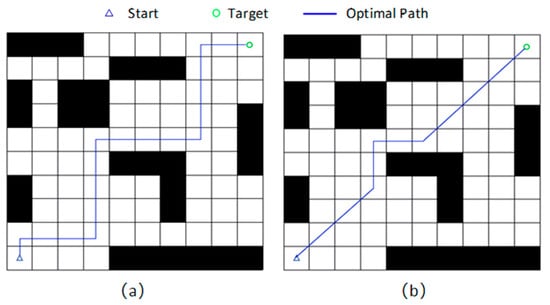
Figure 1.
Distance Representation in Raster Maps; (a): Manhattan grid path; (b): Euclidean grid path.
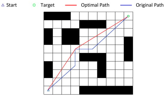
Figure 2.
Path Inflection Point Optimization.
2.2. Improvements to the A* Algorithm
To enhance the rationality and feasibility of path generation by the A* algorithm in complex environments, this paper optimizes the traditional A* algorithm in three aspects: improving the heuristic function, optimizing the cost function, and introducing the Floyd algorithm for path smoothing. These enhancements boost the search efficiency, path quality, and motion controllability of the path-planning algorithm, providing a superior global path foundation for subsequent integration with the DWA algorithm.
2.2.1. Improving the Heuristic Function
In traditional A* algorithms, the heuristic function typically employs Euclidean distance or Manhattan distance to estimate the cost from the current node to the goal node. However, these static estimation methods fail to account for environmental complexity and path pass ability, often resulting in inefficient searches or suboptimal paths. To address this, this paper proposes an improved weighted dynamic heuristic function, formulated as follows:
Among these, ω serves as the heuristic weighting factor, enabling flexible transition of the search strategy from “shortest path priority” to “rapid target convergence” by adjusting its value, Where
- When ω = 1: This corresponds to standard A*, guaranteeing optimality, but search efficiency may be low.
- When ω > 1: The search becomes more biased toward the target direction, significantly accelerating search speed but potentially sacrificing global optimality.
- When ω < 1: The search becomes overly conservative and impractical, as underestimating costs may cause the search to fail to converge.
Additionally, to enhance the adaptability of the heuristic function, the ω value is dynamically increased in areas with high obstacle density. This makes the search more inclined to avoid high-risk zones, thereby improving path safety. Based on the statically set ω value, adjustments are made according to obstacle density:
among them:
- denotes the dynamic weight of node n;
- is the base weight (constant);
- D(n) represents the obstacle density around the current node;
- k is the density influence factor.
Increasing the weight of high-density areas accelerates escape from complex environments, thereby improving search efficiency.
2.2.2. Cost Function Optimization
In the traditional A* algorithm, the cost function typically represents the cumulative path distance from the starting point to the current node n. This distance is the sum of all distances between previously traversed nodes along the path, usually accumulated in unit grid increments. Its calculation is as follows:
Here, denotes the distance from the previous node to the current node, typically set to 1 or . While this method is computationally simple, it fails to account for path motion continuity, resulting in generated paths with excessive sharp turns and abrupt angles that often fail to meet the trajectory tracking requirements of actual AGVs. To enhance path executability and smoothness, this paper introduces a turning penalty term to the traditional cost function. The optimized cost function is as follows:
among them:
- : Represents the change in angle between the current path’s turning angle and the angle of the preceding path segment;
- λ: Steering penalty weighting factor, used to control the degree to which angle changes affect the cost.
In the specific implementation, the steering angle can be calculated using the coordinates of the previous node and the current node:
Calculate the difference between the current angle and the previous path direction:
Figure 2 shows the changes in path inflection points after cost function optimization.
After implementing this feature, the search process will prioritize paths with fewer angular changes, reducing the number of turning points to generate smoother paths with more natural transitions.
2.2.3. Introduction of Floyd’s Algorithm for Path Smoothing
Paths generated by traditional A* algorithm planning typically consist of sequences of discrete grid nodes, connected by straight line segments. This approach often results in redundant nodes and frequent path turns. While such paths ensure reachability, the frequent turns impose significant mechanical loads on AGVs during operation. This leads to amplified path tracking errors and reduced motion control precision, making it difficult to meet the demands for real-time, efficient, and smooth trajectory tracking.
To address the aforementioned issues, this study introduces the Floyd algorithm (Floyd path optimization algorithm) to perform post-processing on the discrete paths generated by the traditional A* algorithm. This eliminates unnecessary redundant nodes in the path, reduces the number of sharp turns, and enhances both the smoothness of motion and the practical operability of the path. The Floyd path smoothing algorithm employs a segment-based direct connection detection approach to retain essential turning points and critical nodes, significantly simplifying the path structure and achieving smooth path optimization.
The specific steps of the Floyd path smoothing algorithm are described as follows:
- (1)
- Initialize the path sequence:
- (2)
- Determine the feasibility of connecting andIf feasible, remove the intermediate node , and update the path length to n − 1;If not feasible, retain node and increment the node index: i = i + 1.
- (3)
- Repeat step (2) until the subscript i ≥ path length − 1;
- (4)
- The final sequence of paths obtained after smoothing optimization:
The introduction of Floyd’s path smoothing algorithm for secondary optimization of A* algorithm output paths not only effectively reduces redundant nodes and unnecessary turning points in the path, minimizing steering impact and trajectory tracking errors during AGV movement, but also offers advantages of simple algorithm implementation and high computational efficiency. This makes it particularly suitable for real-time path planning and practical AGV control requirements in complex environments. The introduction of this method lays a solid foundation for enhancing AGV real-time control and path execution efficiency, as well as for the deep integration of subsequent path-planning algorithms with motion control strategies.
In summary, compared to the traditional A* algorithm, the improved algorithm proposed in this paper effectively reduces redundant nodes and inflection points, generating smoother and more executable global paths.
3. Analysis of the DWA Algorithm
3.1. Traditional DWA Algorithm
The Dynamic Window Algorithm is a sampling-based real-time local path-planning algorithm widely applied in obstacle avoidance and target tracking tasks for mobile robots in dynamic environments. Its core principle involves sampling velocity space to select an optimal velocity pair that enables the robot to both avoid obstacles and move toward the target, while accounting for kinematic and dynamic constraints. Unlike traditional grid-based or graph-search path planning, DWA performs optimization directly at the velocity control layer, emphasizing “reachability trajectories” and “real-time control”.
Its main principle is as follows:
- (1)
- Control input spatial sampling
In actual operation, the robot possesses two degrees of freedom for control: linear velocity and angular velocity , whose changes are constrained by the maximum acceleration limit.
Robot Key Parameters [26]: Linear velocity, ; angular velocity, ; Maximum linear acceleration,; Maximum angular acceleration,; Control cycle, .
The speed range the robot can achieve in the next cycle is:
This velocity space is termed the “dynamic window”, representing the set of feasible control inputs permitted by the intrinsic dynamics at the current moment. DWA will perform discrete sampling of multiple velocity pairs within this window for subsequent trajectory simulation and evaluation.
- (2)
- Trajectory Prediction Model
For each set of sampled velocity pairs , DWA employs a kinematic model to simulate and predict their short-term motion trajectories, typically over a prediction time of 1 to 3 s. For non-omnidirectional differential drive or Mecanum wheel robots, their predictive models often employ nonlinear systems of the following form:
After performing time-step predictions on each set of velocity commands consecutively, a sequence of discrete trajectory points is obtained, referred to as the candidate trajectory set. Each trajectory represents the robot’s path over a future period of time under that specific velocity pair.
- (3)
- Trajectory Evaluation and Objective Function Design
DWA scores and ranks each candidate trajectory using an evaluation function, selecting the speed corresponding to the highest-scoring trajectory as the control output. The traditional DWA evaluation function consists of three main components:
among them:
- heading: Angular deviation of the trajectory endpoint relative to the target point, used to measure target attractiveness;
- dist: Minimum distance between the trajectory and obstacles, reflecting safety;
- velocity: Linear velocity of the trajectory endpoint, encouraging high-speed movement.
The three evaluation metrics are weighted and summed after undergoing regularization processing. The weights are user-preset to regulate the trade-off between safety, goal-orientedness, and efficiency. The evaluation function can also be extended to incorporate dimensions such as energy consumption and curvature, enhancing its environmental adaptability and robustness.
- (4)
- Control Output and Real-Time Execution
After selecting the optimal trajectory corresponding to , DWA will use this velocity pair as the execution command for the robot’s next control cycle. Due to the high control frequency of DWA, the system can achieve continuous path adjustment and dynamic obstacle avoidance through rapid resampling and trajectory evaluation, even when the target moves or new obstacles appear in the environment.
The essence of DWA is to transform the local path-planning problem into an online control input search and optimization problem, enabling real-time planning through finite sampling in velocity space and short-term prediction.
However, this method lacks a global perspective, making it prone to local optima (such as the L-shaped obstacle dilemma). Issues like coarse sampling strategies and overly simplistic evaluation functions also limit its performance in complex environments. Therefore, this paper further improves the DWA algorithm to enhance its intelligence and robustness.
3.2. Improving the DWA Algorithm
Although traditional DWA algorithms exhibit excellent real-time performance and obstacle avoidance capabilities, they still face three bottlenecks in complex dynamic environments: (1) overly simplified evaluation function design that fails to comprehensively measure dynamic risks and path rationality; (2) susceptibility to deadlock in local optima (e.g., L-shaped obstacles), leading to loss of global guidance; (3) Coarse velocity sampling strategies lead to insufficient trajectory space coverage or computational redundancy. To address these limitations, this paper systematically optimizes DWA through the following three approaches.
3.2.1. Optimization and Intelligence of Evaluation Functions
Traditional DWA employs a static weighting evaluation function that comprehensively considers target distance, obstacle distance, and velocity magnitude, as described in Equation (15). While this form features a simple structure, it suffers from fixed weights that cannot dynamically adapt to varying environments. Particularly in complex scenarios, a single metric fails to achieve effective trade-offs, leading to evaluation biases.
To enhance the algorithm’s perception and decision-making capabilities, this paper introduces an adaptive weighting mechanism and a risk perception factor to intelligently extend the evaluation function. The improved objective function is as follows:
among them:
- : Weight parameters dynamically adjusted based on the current environment;
- : The reciprocal of the deviation from the target direction;
- : Indicates the distance to the nearest obstacle;
- : Indicates the current linear velocity;
- : For the newly added dynamic risk perception factor, generated based on the density of obstacles ahead along the trajectory and the predicted velocity field, it is used to penalize potentially high-risk trajectories.
The specific calculation formula for risk perception factor is:
among them:
- : To predict the minimum distance (m) between the trajectory and obstacles in the time domain;
- : To predict the shortest collision time (s) in the time domain, set it to +∞ if there is no collision risk;
- : For the risk factors, the minimum distance and collision time weights satisfy = 1.
To achieve environmental adaptability, weights are dynamically adjusted based on local obstacle density and global path deviation , calculated as follows:
among them:
- : Normalized heading error;
- : The normalized value of obstacle density within a local window;
- : To normalize terminal velocity;
- : Normalized risk perception value;
- : Coefficient regulating the dynamic variation range of weights.
The adaptive adjustment of certain weights in this paper is implemented as follows:
Here, represents the degree of deviation of the current trajectory from the global path, and denotes the local density of obstacles.
This optimization mechanism enables DWA to prioritize speed and target direction in open areas while emphasizing safety in crowded environments, effectively enhancing the algorithm’s environmental adaptability.
3.2.2. Local Optimality Problem and L-Shaped Obstacle Lockup Avoidance
When encountering complex obstacle structures (such as L-shaped blind spots), traditional DWA often gets stuck in local optima and fails to escape due to its reliance solely on local velocity sampling and short-term trajectory evaluation. To overcome this issue, this paper introduces an auxiliary target guidance mechanism that applies “soft constraints” to local paths based on global path-planning results.
The specific approach is as follows:
- (1)
- Extract the next target reference point (sub-goal) for the current stage from the global path generated by A*;
- (2)
- Input this sub-goal as the target direction into the DWA evaluation function, i.e., update the heading term:where represents the current velocity direction, and denotes the direction from the current position to the sub-target;
- (3)
- When detecting a trajectory stuck in an infinite loop (e.g., constant velocity, repetitive positioning), trigger the obstacle avoidance resampling mechanism. This expands the sampling window and temporarily suppresses velocity dimension sampling to guide the robot out of oscillation.
Figure 3a shows an AGV facing an L-shaped obstacle, where it tends to get stuck in a local optimum. By updating the heading parameter and other optimization methods, Figure 3b demonstrates that the optimized AGV is no longer constrained by the L-shaped obstacle and successfully navigates around it.
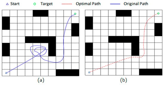
Figure 3.
Comparison of DWA Algorithm Performance Before and After Improvement; (a): Traditional DWA algorithm; (b): Optimized DWA algorithm.
By introducing sub-objectives and a deadlock detection mechanism, the DWA algorithm achieves significantly enhanced traversal robustness and global guidance capabilities within complex obstacle structures.
3.2.3. Sampling Strategy Optimization: Non-Uniform + Adaptive Sampling
Traditional DWA employs an equidistant uniform sampling strategy in velocity space. While simple to implement, it suffers from two significant issues:
- (1)
- Fixed sampling density may result in insufficient spatial coverage for certain trajectories, compromising decision-making accuracy;
- (2)
- Low sampling efficiency during low-speed operation or in confined spaces leads to excessive redundant computational load.
To enhance sampling quality and efficiency, this paper proposes a mechanism combining non-uniform sampling with adaptive resolution adjustment. Its primary optimizations include:
- (1)
- Non-uniform sampling distribution: Increases sampling density in regions near the target direction within velocity space while reducing sampling points in areas distant from the target direction
- (2)
- Velocity-obstacle density coupling adjustment mechanism: Adjusts sampling resolution based on the current obstacle density , enabling finer sampling in densely obstructed zones:
The function is a monotonically decreasing function.
Dynamic Sampling Range Expansion Mechanism: If all trajectories within the current sampling window are deemed invalid, the velocity sampling boundaries are automatically expanded to broaden the exploration range and prevent getting stuck in a “no feasible solution” state. This strategy ensures effective coverage of the trajectory space while significantly reducing invalid sampling points, thereby enhancing the DWA algorithm’s response efficiency and computational stability in highly dynamic scenarios.
In summary, compared to traditional DWA, the improvements proposed in this paper effectively avoid local optima traps while enhancing the real-time performance and stability of dynamic obstacle avoidance.
4. Design of an Improved A* and DWA Fusion Algorithm
To balance the optimality of global paths with the real-time obstacle avoidance capability of local paths, this paper proposes a hybrid path-planning method based on an improved A* algorithm and an improved DWA algorithm, establishing a dual-layer architecture of “global guidance + local obstacle avoidance”. Within this architecture, the enhanced A* algorithm generates the global path skeleton, providing the path framework and sequence of intermediate key points. The enhanced DWA algorithm dynamically adjusts the local motion trajectory during path execution, enabling avoidance of dynamic obstacles and path fine-tuning. This approach enhances the overall feasibility and robustness of the path.
4.1. Integration Mechanism
To achieve global optimal path planning and local real-time obstacle avoidance control for AGVs in complex dynamic environments, this paper integrates the improved A* algorithm with the enhanced DWA algorithm, forming a dual-layer path-planning mechanism where DWA serves as the primary controller and A* provides auxiliary support. The overall system operation flow is illustrated in Figure 3, with specific steps as follows:
- Step 1: Environment Modeling and Parameter Initialization
Create a grid map based on known environmental information, set the starting point, destination, and obstacle distribution, and initialize the AGV’s kinematic parameters, sensor information, and DWA-related control parameters.
- Step 2: Local Path Planning and Velocity Sampling
The DWA module, serving as the system’s main control unit, dynamically samples the current obstacle distribution and velocity space while predicting trajectories based on real-time sensor data. By calculating scores for each sampled trajectory using an improved evaluation function, it selects the optimal control command to achieve real-time obstacle avoidance and local path generation for the AGV.
- Step 3: Movement Execution and Status Update
The AGV moves according to the optimal speed commands output by the DWA module. Simultaneously, the system continuously updates its pose, velocity, and surrounding environmental status, providing input for subsequent trajectory sampling and obstacle avoidance calculations.
- Step 4: Deviation Detection and Trigger Assessment
The system continuously monitors the deviation between the AGV’s current pose and the global reference trajectory. When it detects that the local path is impassable, obstacles have changed, or the position deviation exceeds the threshold, it triggers the global re-planning module.
- Step 5: Global Path Replanning and Smoothness Optimization
Once the trigger conditions are met, the enhanced A* algorithm module is invoked to regenerate the globally optimal path using the latest environmental data. After A* planning completes, the Floyd algorithm is applied to smooth the path and eliminate redundant nodes, yielding a continuous, feasible optimized path.
- Step 6: Path Feedback and Closed-Loop Control
The Floyd-smoothed path is fed back to the DWA module as a new global reference path for velocity sampling and obstacle avoidance planning in the next phase, forming a closed-loop fusion mechanism of “global path guidance—local dynamic correction”. The system iteratively executes steps 2 through 6 until the AGV reaches the target point and completes the task.
Through the aforementioned integrated mechanism, the system achieves adaptive path adjustments during operation in response to environmental changes: the enhanced DWA algorithm ensures real-time path planning and dynamic obstacle avoidance capabilities, while the improved A* algorithm provides global path correction and guarantees optimality. The synergistic combination of both algorithms enables smoother, more efficient, and safer path planning for AGVs in complex mixed environments.
4.2. Fusion Algorithm Flowchart
Figure 4 illustrates the flowchart of the fusion algorithm, providing a visual representation of its process.
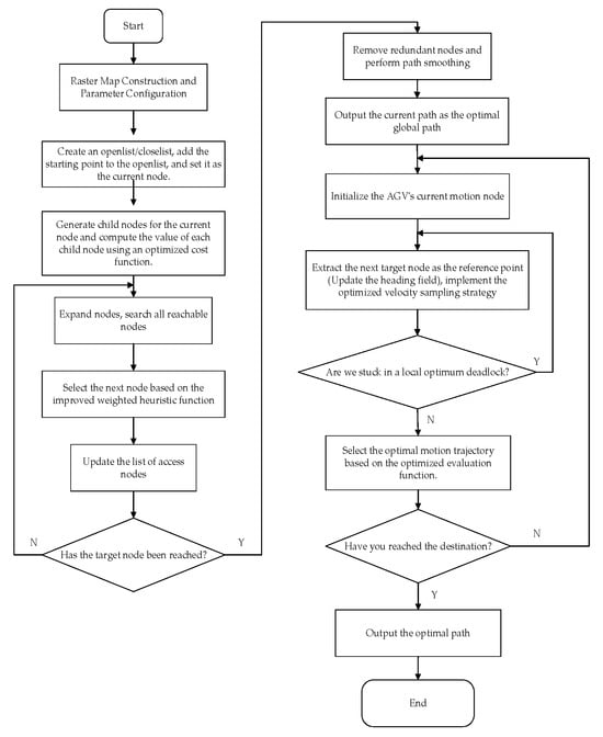
Figure 4.
Fusion Algorithm Flowchart.
5. Algorithm Simulation Verification
To validate the effectiveness and superiority of the proposed algorithm, a two-dimensional grid simulation environment was established on the MATLAB R2024a platform. The experiments were divided into two sets: the first set compared the improved A* algorithm, while the second set compared the fusion of the improved A* and DWA algorithms. The experimental platform operates on Windows 11 with hardware specifications of an Intel i9 processor and 16 GB of memory. Black squares represent trees and forest obstacles, while white areas denote traversable ground paths.
5.1. Experiments on Improving the A* Algorithm
The first set of experiments compared the path-planning performance of the improved A* algorithm proposed in this paper, the traditional A* algorithm, the ACO (ant colony algorithm) algorithm, and the improved A* algorithm proposed in reference [7] under static conditions. The improved A* algorithm proposed in Reference [7] balances search efficiency and path smoothness, representing a dual optimization approach that provides important reference for the experimental methodology in this paper. The ACO algorithm is also one of the mainstream algorithms today, and its global planning performance is also quite good, and it can adapt to the situation of random obstacles.
5.1.1. Improved Experimental Environment and Settings for the A* Algorithm
Obstacles were randomly generated to simulate the complex diversity of forest tree paths, with a spatial density of approximately 20%. To minimize error, simulations were conducted in environments with map sizes of 20 × 20, 30 × 30, and 100 × 100. Ten sets of random experiments were performed for each map size [27], with each set using a square grid map of 1 m side length. Results from multiple experiments are shown in Figure 5 and Figure 6. Following multiple experiments, the key parameter settings for the simulated environment are summarized in Table 1.
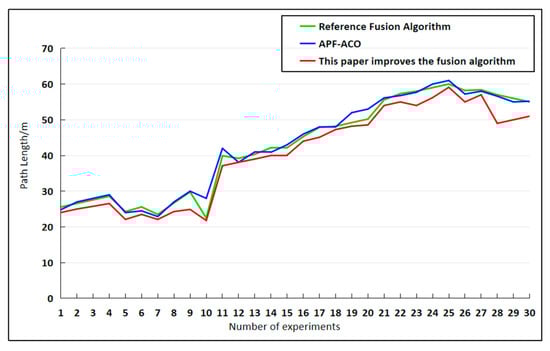
Figure 5.
Path Lengths from 30 Experiments in Three Environments.
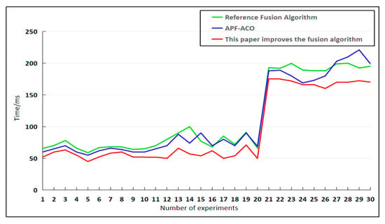
Figure 6.
Time Schedule for 30 Experiments in Three Environments.

Table 1.
Key Parameters.
5.1.2. Simulation Results
As shown in Figure 5 and Figure 6, the 30 sets of experiments demonstrate that the proposed improved A* algorithm exhibits significant advantages in both path length and planning time when obstacles are randomly distributed. The simulation experiments in a model forest obstacle environment are described below. Among them, the gray squares represent the traversed nodes. The references cited in the following figures all correspond to Reference [7]. The data in Table 2 indicate that the improved A* algorithm proposed in this paper outperforms the comparison algorithms across multiple evaluation metrics. In terms of path length, for the 20 × 20, 30 × 30, and 100 × 100 maps, the proposed method achieves reductions of 8.40%, 5.41%, and 4.35% compared with the traditional A* algorithm; 7.31%, 2.63%, and 9.47% relative to the algorithm in [7]; and 4.19%, 1.82%, and 10.64% compared with the ACO algorithm. For planning time, the proposed algorithm achieves reductions of 29.45%, 77.62%, and 37.59% compared with the traditional A*; 17.24%, 74.17%, and 17.83% relative to the algorithm in [7]; and 22.35%, 66.55%, and 55.33% compared with ACO. Regarding the number of inflection points, reductions of 40.00%, 44.44%, and 53.49% are observed relative to the traditional A* algorithm; 40.00%, 37.50%, and 31.03% relative to the algorithm in [7]; and 50.00%, 37.50%, and 50.00% compared with ACO.
For steering angle and search nodes, the improved algorithm also achieves substantial reductions across all map scales, resulting in significantly enhanced search efficiency. Figure 7, Figure 8 and Figure 9 present the corresponding experimental result visualizations. These results collectively validate the comprehensive advantages of the proposed method in terms of path optimality, smoothness, and computational efficiency.
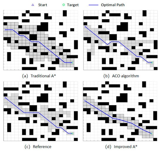
Figure 7.
Simulation results of the A* algorithm on a 20 × 20 grid map.
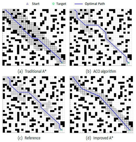
Figure 8.
Simulation results of the A* algorithm on a 30 × 30 grid map.
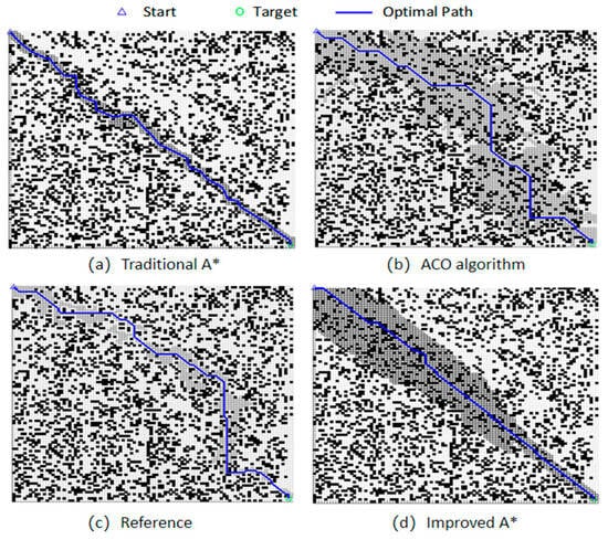
Figure 9.
Simulation results of the A* algorithm on a 100 × 100 grid map.
5.2. Fusion Algorithm Simulation Experiments
In the second group of experiments conducted in a dynamic environment, the proposed improved fusion algorithm was compared with the fusion algorithm from reference [7] and the APF-ACO algorithm in terms of path-planning performance. The fusion algorithm in reference [7] and the APF-ACO algorithm are currently commonly used representative fusion algorithms, and therefore were selected as the subjects of the comparative experiment.
5.2.1. Experimental Environment and Settings for Fusion Algorithms
Obstacles in dynamic environments are randomly generated or customizable, with a 20% probability of occurrence. To minimize error, simulation experiments were conducted on environments with map sizes of 20 × 20 and 30 × 30 and 100 × 100. Each map size underwent 10 sets of random experiments, utilizing square grid maps with a unit cell size of 1 m, incorporating both dynamic and static obstacles.
During the local path-planning phase, this paper employs an improved dynamic window method. Through extensive simulation experiments comparing path smoothness, obstacle avoidance success rate, and average speed under various parameter combinations, an optimal set of weighting parameters was ultimately selected. To balance path safety, global convergence, and real-time performance, the coefficients in the evaluation function are reasonably set: Considering that AGVs need to maintain a certain maneuvering capability when approaching the target point, simply pursuing a direct path to the target is not optimal. Therefore, the target orientation factor weight is set. Since obstacles have undergone expansion processing, ensuring a safety margin, to avoid overly conservative paths leading to excessive length, the obstacle distance factor weight is set. In industrial material handling scenarios, speed efficiency is critical, hence the velocity term weight . Simultaneously, to prevent local optima traps and maintain consistency with the global path, the trajectory deviation factor is introduced. This parameter configuration ensures safety while enhancing obstacle avoidance efficiency and trajectory stability in dynamic environments. Table 3 details the AGV parameter settings for the simulation environment [28].
Table 3.
Initial Parameters for Dynamic Window Method and AGV Parameter Settings.
5.2.2. Analysis of Simulation Results
To analyze the dynamic obstacle avoidance capability and environmental adaptability of the fusion algorithm presented in this paper, three experimental environments were designed for comparison with [7] and APF-ACO: a 20 × 20 grid map and a 30 × 30 grid map and a 100 grid map each incorporating dynamic and static obstacles.
As shown in Figure 10 and Figure 11, the proposed fusion algorithm outperforms the comparison algorithm in both path length and planning time within complex environments containing both dynamic and static obstacles. Although real-time path planning in dynamic environments poses greater challenges in terms of performance and stability, the algorithm effectively reduces path distance and shortens planning time through its dual-layer optimization mechanism that combines global and local approaches.
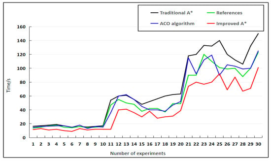
Figure 10.
Time Planning for 30 Experiments in Two Environments.
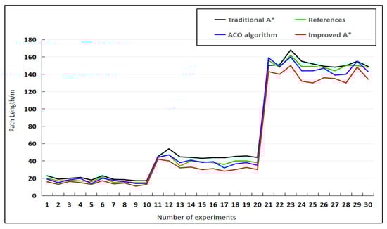
Figure 11.
Path Lengths from 30 Experiments in Two Environments.
The following is a simulation experiment of the fusion algorithm. The solid blue circle represents the robot’s current position. The red arrows indicate the movement direction of dynamic obstacles, while the red short lines represent the movement paths of moving obstacles.
Based on the comprehensive analysis of simulation results from Figure 12, Figure 13, Figure 14, Figure 15, Figure 16, Figure 17, Figure 18, Figure 19, Figure 20, Figure 21, Figure 22, Figure 23, Figure 24, Figure 25 and Figure 26, the proposed improved fusion algorithm demonstrates significantly superior performance compared to the fusion algorithm in [7] and the APF-ACO algorithm across all three map scales: 20 × 20, 30 × 30, and 100 × 100.
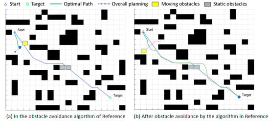
Figure 12.
Simulation Results of the 20 × 20 Map Fusion Algorithm; (a): The state of the 20-map document [7] fusion algorithm in obstacle avoidance; (b): The state of the 20-map document [7] fusion algorithm after obstacle avoidance.
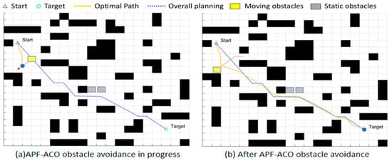
Figure 13.
Simulation Results of the 20 × 20 Map Fusion Algorithm; (a): The status of APF-ACO during obstacle avoidance in the 20th map; (b): The state of APF-ACO after obstacle avoidance in the 20th map.
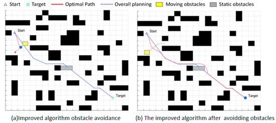
Figure 14.
Simulation Results of the 20 × 20 Map Fusion Algorithm; (a): The state of the improved fusion algorithm in obstacle avoidance within the 20-map environment; (b): The state following obstacle avoidance after implementing the improved fusion algorithm on the 20-map.
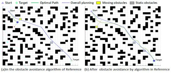
Figure 15.
Simulation Results of the 30 × 30 Map Fusion Algorithm; (a): The state of the 30-map document [7] fusion algorithm in obstacle avoidance; (b): The state of the 30-map document [7] fusion algorithm after obstacle avoidance.
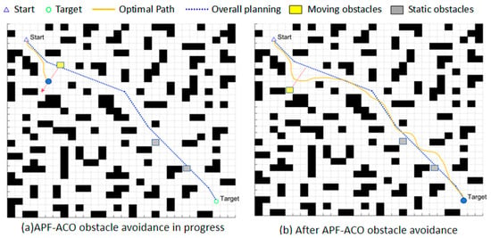
Figure 16.
Simulation Results of the 20 × 20 Map Fusion Algorithm; (a): The status of APF-ACO during obstacle avoidance in the 30th map; (b): The state of APF-ACO after obstacle avoidance in the 30th map.
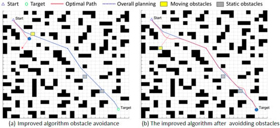
Figure 17.
Simulation Results of the 20 × 20 Map Fusion Algorithm; (a): The state of the improved fusion algorithm in obstacle avoidance within the 30-map environment; (b): The state following obstacle avoidance after implementing the improved fusion algorithm on the 30-map.
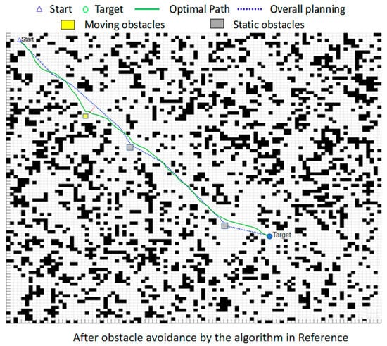
Figure 18.
Simulation Results of the 100 × 100 Map Fusion Algorithm: the state of the 100-map document [7] fusion algorithm after obstacle avoidance.
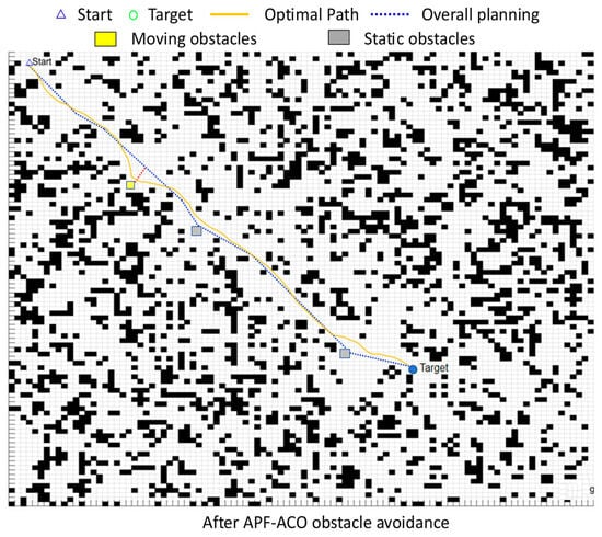
Figure 19.
Simulation Results of the 100 × 100 Map Fusion Algorithm: the state of APF-ACO after obstacle avoidance in the 100th map.
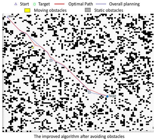
Figure 20.
Simulation Results of the 100 × 100 Map Fusion Algorithm: the state following obstacle avoidance after implementing the improved fusion algorithm on the 100-map.
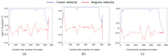
Figure 21.
Speed Variation Curve of the 20 × 20 Map Fusion Algorithm: (a): Speed variation in the fusion algorithm in [7]; (b): speed variation in the fusion APF-ACO; (c): speed variation in the fusion algorithm in this paper.
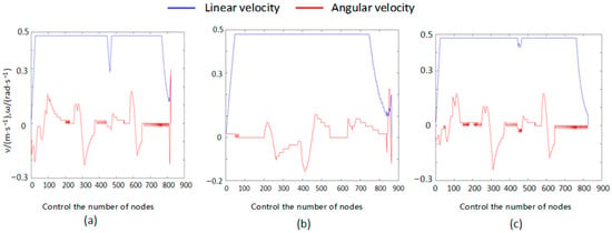
Figure 22.
Speed Variation Curve of the 30 × 30 Map Fusion Algorithm: (a): Speed variation in the fusion algorithm in [7]; (b): speed variation in the fusion APF-ACO; (c): speed variation in the fusion algorithm in this paper.
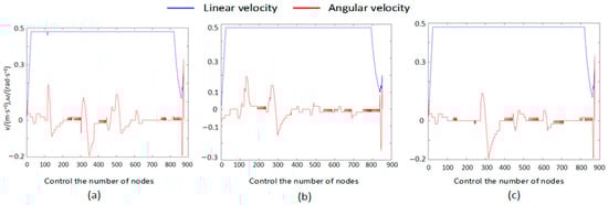
Figure 23.
Speed Variation Curve of the 100 × 100 Map Fusion Algorithm: (a): speed variation in the fusion algorithm in [7]; (b): speed variation in the fusion APF-ACO; (c): speed variation in the fusion algorithm in this paper.
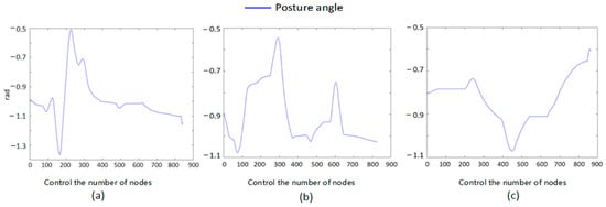
Figure 24.
20 × 20 Map Fusion Algorithm Attitude Angles: (a): attitude angle of AGV using fusion algorithm from [7]; (b): attitude angle of AGV using the fusion APF-ACO; (c): attitude angle of AGV using the fusion algorithm in this paper.
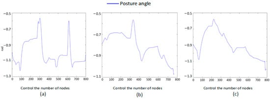
Figure 25.
30 × 30 Map Fusion Algorithm Attitude Angles: (a): Attitude angle of AGV using; fusion algorithm from [7]; (b): attitude angle of AGV using the fusion APF-ACO; (c): attitude angle of AGV using the fusion algorithm in this paper.
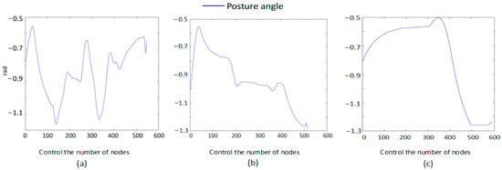
Figure 26.
100 × 100 Map Fusion Algorithm Attitude Angles: (a): Attitude angle of AGV using; fusion algorithm from [7]; (b): attitude angle of AGV using the fusion APF-ACO; (c): attitude angle of AGV using the fusion algorithm in this paper.
Although the global planning of the three methods was nearly identical before incorporating dynamic and static obstacles—as they all followed the A* global path framework—the performance differences between the algorithms became markedly apparent once dynamic obstacles were introduced into the environment, requiring the AGV to frequently execute local replanning. Figure 12, Figure 13, Figure 14, Figure 15, Figure 16, Figure 17, Figure 18, Figure 19, Figure 20, Figure 21, Figure 22, Figure 23, Figure 24, Figure 25 and Figure 26 clearly demonstrate that the proposed fusion algorithm exhibits smoother and more stable curves for linear velocity, angular velocity, and attitude angle changes during local obstacle avoidance. Particularly in the velocity curves of Figure 21, Figure 22 and Figure 23, our algorithm avoids the frequent velocity spikes and significant oscillations observed in the fusion algorithms from [7] and the APF-ACO fusion algorithm. In the attitude angle curves of Figure 24, Figure 25 and Figure 26, our algorithm converges faster after obstacle avoidance and exhibits more continuous and natural attitude adjustments, clearly outperforming the comparison algorithms.
These graphical conclusions are further validated by the quantitative data in Table 4: On 20 × 20, 30 × 30, and 100 × 100 maps, our fusion algorithm reduces path length by 6.10%, 7.01%, and 7.54%, respectively, compared to the fusion method in [7], while reducing planning time by 19.56%, 9.01%, and 6.10%, respectively. Compared to the APF-ACO fusion algorithm, path lengths decreased by 7.54%, 9.01%, and 11.00%, respectively, while planning times decreased by 22.47%, 9.64%, and 24.79%, respectively. The fusion algorithm also demonstrated consistent advantages in terms of turning angles.
In summary, when dynamic obstacles are introduced, the improved DWA in this paper plays a crucial role at the local planning level. This enables the fusion algorithm to maintain global path consistency while demonstrating stronger dynamic obstacle avoidance capabilities and enhanced motion stability.
6. Conclusions
This study proposes a hybrid path-planning framework that integrates an improved A* algorithm with an enhanced Dynamic Window Approach (DWA) for forestry AGVs operating in rugged and dynamic environments. The improved A* employs a dynamically weighted heuristic, a steering-penalty cost model, and Floyd-based smoothing, enabling the generation of smoother and more executable global paths. The enhanced DWA incorporates adaptive weight adjustment, a dynamic risk-perception factor, a subgoal-guidance term, and a non-uniform adaptive sampling strategy to improve real-time obstacle avoidance and motion stability.
Through tight global–local coupling, the proposed framework achieves significant performance gains. Across 20 × 20, 30 × 30, and 100 × 100 grid maps, average path length is reduced by 6.82%, 8.13%, and 21.78%; planning time is reduced by 21.02%, 16.65%, and 9.33%; and total steering angle decreases by 100°, 487.5°, and 587.5°, respectively. These results verify the effectiveness of the hybrid approach in improving path optimality, computational efficiency, and trajectory smoothness in complex forest-like environments.
Overall, the proposed method provides a practical and robust solution for intelligent forestry navigation tasks and holds strong potential for broader applications in agriculture, industrial logistics, and other scenarios involving mixed static–dynamic obstacles.
Author Contributions
Conceptualization, K.W.; Methodology, K.W.; Software, K.W.; Validation, K.W.; Formal analysis, M.Z.; Investigation, K.W. and M.Z.; Resources, J.Z.; Data curation, M.Z.; Writing—original draft, K.W.; Writing—review & editing, S.L. and J.Z.; Supervision, S.L. and J.Z.; Project administration, S.L.; Funding acquisition, S.L. All authors have read and agreed to the published version of the manuscript.
Funding
This research was funded by the Beijing Institute of Graphic Communication, project “Research and development of working pressure direct monitoring for flat die cutting machine”, grant number Ea202406, and by the Project of Construction and Support for High-level Innovative Teams of Beijing Municipal Institutions, project “Key technologies and equipment for MLCC roll-to-roll precision coated printing”, grant number BPHR20220107, and by the Beijing Institute of Graphic Communication, project “Beijing Key Laboratory of Digital Printing Equipment Construction Project”, grant number KYCPT202508. The APC was funded by the Beijing Institute of Graphic Communication.
Data Availability Statement
The data supporting the reported results are not publicly available due to corporate privacy and laboratory confidentiality agreements.
Acknowledgments
The authors gratefully acknowledge the support of the Beijing Institute of Graphic Communication. No generative AI tools were used in the preparation of this manuscript; the authors are fully responsible for its content.
Conflicts of Interest
The authors declare no conflicts of interest. The funders had no role in the design of the study; in the collection, analyses, or interpretation of data; in the writing of the manuscript; or in the decision to publish the results.
Abbreviations
The following abbreviations are used in this manuscript:
| AGV | Automated Guided Vehicle |
| DWA | Dynamic Window Approach |
| A* | A-star Algorithm |
| ACO | Ant Colony Optimization |
| APF-ACO | Artificial Potential Field-Ant Colony Optimization |
References
- Kiga, Y.; Sugasawa, Y.; Sakai, T.; Nemoto, T.; Iwase, M. Development of roCaGo for Forest Observation and Forestry Support. Forests 2025, 16, 1067. [Google Scholar] [CrossRef]
- Lee, H.-S.; Kim, G.-H.; Ju, H.-S.; Mun, H.-S.; Oh, J.-H.; Shin, B.-S. Global Navigation Satellite System/Inertial Navigation System-Based Autonomous Driving Control System for Forestry Forwarders. Forests 2025, 16, 647. [Google Scholar] [CrossRef]
- Wu, Y.; Zhong, S.; Ma, Y.; Zhang, Y.; Liu, M. Application of SLAM-Based Mobile Laser Scanning in Forest Inventory: Methods, Progress, Challenges, and Perspectives. Forests 2025, 16, 920. [Google Scholar] [CrossRef]
- Zhao, J.; Zhang, Y.; Ma, Z.; Ye, Z. Improvement and validation of A* algorithm for AGV path planning. Comput. Eng. Appl. 2018, 54, 217–223. [Google Scholar]
- Yang, M.; Li, N. Mobile robot path planning using an improved A* algorithm. Mech. Sci. Technol. 2022, 41, 795–800. [Google Scholar] [CrossRef]
- Liu, C.; Mao, Q.; Chu, X.; Xie, S. An Improved A-Star Algorithm Considering Water Current, Traffic Separation and Berthing for Vessel Path Planning. Appl. Sci. 2019, 9, 1057. [Google Scholar] [CrossRef]
- Zhao, Q.; Shi, Y. Real-time path planning and obstacle avoidance of AGV based on fusion of improved A* algorithm and DWA. Mod. Manuf. Eng. 2025, 91–98. [Google Scholar]
- Li, P.; Zhou, L.; Chen, Z. Dynamic Obstacle Avoidance Algorithm in Dynamic Environments Based on Fusion of DWA and Artificial Potential Field. Comput. Eng. Appl. 2025, 61, 98–105. [Google Scholar] [CrossRef]
- Liao, X.; Wang, Y.; Xuan, Y.; Wu, D. AGV Path Planning Model Based on Reinforcement Learning. In Proceedings of the 2020 Chinese Automation Congress (CAC), Shanghai, China, 6–8 November 2020; pp. 6722–6726. [Google Scholar] [CrossRef]
- Pratama, A.Y.; Ariyadi, M.R.; Tamara, M.N.; Purnomo, D.S.; Ramadhan, N.A.; Pramujati, B. Design of Path Planning System for Multi-Agent AGV Using A* Algorithm. In Proceedings of the 2023 International Electronics Symposium (IES), Denpasar, Indonesia, 8–10 August 2023; pp. 335–341. [Google Scholar] [CrossRef]
- Yang, X.; Yuan, Z.; Bai, Y.; Au, P. A double-neighborhood expansion A* path planning algorithm. Mech. Sci. Technol. 2025, 44, 484–495. [Google Scholar] [CrossRef]
- Gao, J.; Xu, X.; Pu, Q.; Liang, L.; Niu, Y. A Hybrid Path Planning Method Based on Improved A* and CSA-APF Algorithms. IEEE Access 2024, 12, 39139–39151. [Google Scholar] [CrossRef]
- Wang, H.B.; Yin, P.H.; Zheng, W.; Wang, H.; Zuo, J.S. Mobile Robot Path Planning Based on Improved A* Algorithm and Dynamic Window Approach. Robot 2020, 42, 346–353. [Google Scholar] [CrossRef]
- Liu, Y.; Zhang, H.; Chen, X.; Wang, J. Adaptive sampling-based dynamic window approach for mobile robot path planning in dense obstacle environments. J. Intell. Robot. Syst. 2022, 105, 45. [Google Scholar]
- Kim, J.; Yang, G.H. Improved Dynamic Window Approach Using Reinforcement Learning in Dynamic Environments. Int. J. Control. Autom. Syst. 2024, 22, 1289–1302. [Google Scholar] [CrossRef]
- Cao, L.; Tang, L.; Cao, S.; Sun, Q.; Zhou, G. Smooth Optimised A*-Guided DWA for Mobile Robot Path Planning. Appl. Sci. 2025, 15, 6956. [Google Scholar] [CrossRef]
- Sun, Y.; Liu, J.; Kong, X.; Zhang, F.; Wu, Y.; Li, L. Research on Path Planning of Mobile Robot by Fusing A* and DWA Algorithms. In Proceedings of the 2023 8th International Conference on Intelgent Computing and Signal Processing (ICSP), Xi’an, China, 21–23 April 2023; pp. 1467–1471. [Google Scholar]
- Wu, B.; Chi, X.; Zhao, C.; Zhang, W. Dynamic Path Planning for Mobile Robots Based on Improved A* and Dynamic Window Approach. Mathematics 2023, 11, 4635. [Google Scholar]
- Liu, W.; Chu, C.; Xiao, M. An improved A* algorithm based on dual optimization of time and path. Manuf. Autom. 2023, 45, 173–177. [Google Scholar]
- Li, Y.; Liu, Y. Research on Path Planning Based on the Integrated Artificial Potential Field-Ant Colony Algorithm. Appl. Sci. 2025, 15, 4522. [Google Scholar] [CrossRef]
- Wu, T.; Zhang, Z.; Jing, F.; Gao, M. A Dynamic Path Planning Method for UAVs Based on Improved Informed-RRT* Fused Dynamic Windows. Drones 2024, 8, 539. [Google Scholar] [CrossRef]
- Shao, Q.; Miao, J.; Liao, P.; Liu, T. Dynamic Scheduling Optimization of Automatic Guide Vehicle for Terminal Delivery under Uncertain Conditions. Appl. Sci. 2024, 14, 8101. [Google Scholar] [CrossRef]
- Xu, Y.; Liu, W.; Yuan, H. Multi-AGV Scheduling and Path Planning Based on an Improved Ant Colony Algorithm. Vehicles 2025, 7, 102. [Google Scholar] [CrossRef]
- Yang, G.; Li, M.; Gao, Q. Multi-Automated Guided Vehicles Conflict-Free Path Planning for Packaging Workshop Based on Grid Time Windows. Appl. Sci. 2024, 14, 3341. [Google Scholar] [CrossRef]
- Hart, P.E.; Nilsson, N.J.; Raphael, B. A formal basis for the heuristic determination of minimum cost paths. IEEE Trans. Syst. Sci. Cybern. 1968, 4, 100–107. [Google Scholar] [CrossRef]
- Zhao, Y.; Zhang, Z. Safe mobile robot path planning based on fusion of improved A* and DWA. Modul. Mach. Tools Autom. Manuf. Tech. 2025, 37–43. [Google Scholar]
- Liu, Z.; Zhao, J.; Liu, C.; Lai, K.; Wang, X. Indoor mobile robot path planning based on improved A* algorithm. Comput. Eng. Appl. 2021, 57, 186–190. [Google Scholar]
- Sang, W.; Yue, Y.; Zhai, K.; Lin, M. Research on AGV Path Planning Integrating an Improved A* Algorithm and DWA Algorithm. Appl. Sci. 2024, 14, 7551. [Google Scholar] [CrossRef]
Disclaimer/Publisher’s Note: The statements, opinions and data contained in all publications are solely those of the individual author(s) and contributor(s) and not of MDPI and/or the editor(s). MDPI and/or the editor(s) disclaim responsibility for any injury to people or property resulting from any ideas, methods, instructions or products referred to in the content. |
© 2025 by the authors. Licensee MDPI, Basel, Switzerland. This article is an open access article distributed under the terms and conditions of the Creative Commons Attribution (CC BY) license.