Article

Patch-Wise Prediction and Interpretable Analysis of Pine Wilt Disease Occurrence

Artificial Intelligence Lab, Department of Computer Science and Engineering, Jeonbuk National University, Jeonju 54896, Republic of Korea
*
Author to whom correspondence should be addressed.
Forests 2025, 16(6), 935; https://doi.org/10.3390/f16060935
Submission received: 27 March 2025 / Revised: 30 May 2025 / Accepted: 31 May 2025 / Published: 2 June 2025
(This article belongs to the Special Issue Management of Forest Pests and Diseases—2nd Edition)

Abstract

:
The pine wood nematode, a microscopic worm-like organism, is the primary cause of Pine Wilt Disease (PWD), a serious threat to pine forests, as infected trees can die within a few months. In this study, we aim to predict the occurrence of PWD by leveraging geographical and meteorological features, with a particular focus on incorporating interpretability through explainable AI (XAI). Unlike conventional models that utilize features from a single point of location, our approach considers surrounding environmental factors (patches) and employs a channel grouping mechanism to aggregate features effectively, enhancing prediction accuracy. Experimental results demonstrate that the proposed model based on convolutional neural network (CNN) outperforms traditional point-wise models, achieving a 9.7% higher F1-score. Experimental results show that data augmentation further improved performance, while interpretability analysis identified precipitation and temperature-related features as the most significant contributors. The developed CNN model provides a robust and interpretable framework, offering valuable insights into the spatial and environmental dynamics of PWD occurrence.

1. Introduction

Pine Wilt Disease (PWD), caused primarily by the pinewood nematode (Bursaphelenchus xylophilus), is a devastating threat to forest ecosystems, particularly those dominated by Pinus species. In Asia, including South Korea, China, Japan, and Taiwan, PWD has emerged as the most destructive forest disease [1], inflicting severe economic and ecological damage. The disease is transmitted naturally by vectors such as long-horned beetles and can also spread anthropogenically through human activities, making its control complex and multidimensional.
The spread and development of pests and disease pathogens, including those responsible for PWD, are strongly influenced by environmental conditions. Prediction methods for pest and disease outbreaks often focus on the relationship between the life cycles of pathogens or pests and key meteorological factors. For instance, when conditions such as temperature, precipitation, or humidity align with the biological requirements of a pest or pathogen, the likelihood of an outbreak increases significantly. Leveraging observed or forecasted environmental data, researchers have been able to estimate the probability and potential extent of such outbreaks [2,3,4]. Moreover, climate change, driven by global warming, has intensified these dynamics. Shifts in temperature, rainfall patterns, and humidity not only alter vegetation distributions [5,6] but also indirectly impact pest populations and invasive pathogens by transforming the ecosystems they depend on.
Accurate prediction models for PWD are critical for developing targeted control measures and efficiently allocating limited resources. Previous research has employed various machine learning techniques and spatial models, including random forest models [7], logistic regression (aka MaxEnt) models [8], ensemble approaches integrating multiple algorithms [9,10], and the CA–Markov model [11]. Ensemble models combining MaxEnt and CLIMEX have been particularly effective in identifying high-risk areas under current and future climatic scenarios, revealing significant concentrations in low-altitude areas and highlighting the potential for further spread through insect vectors in South Korea [9]. Additionally, regression analysis combined with MaxEnt modeling has been used to estimate the natural spread boundary and predict PWD distribution, emphasizing the role of seasonal climatic factors and anthropogenic influences in the disease’s propagation [10]. Basically, research [7,8,9,10] has primarily utilized a point-wise approach, concentrating on the environmental features of individual locations. To incorporate spatial dependencies, the CA–Markov model [11] has been applied to predict PWD occurrences at a geospatial scale, analyzing factors such as terrain, population density, and traffic. These models have demonstrated high accuracy and revealed significant spatiotemporal patterns, including trends in the spread of PWD to previously unaffected high-altitude and steep-slope areas [11]. However, effective CA–Markov modeling requires spatiotemporal input data with sufficient quality at an appropriate scale. On the other hand, studies related to the detection of PWD or the analysis of pine disease using geospatial images from satellite remote sensing or unmanned aerial vehicles [12,13,14,15] have naturally leveraged spatial dependencies, as these are crucial for image-based analysis. Notably, a study [15] leveraged not only spatial dependencies but also spatiotemporal dependencies by employing random point process models. Such studies provide valuable insights into the dynamics of PWD but also underscore the need for a continuous refinement of predictive models to address the evolving nature of the disease. Building upon these studies, we aim to enhance predictive accuracy and applicability, contributing to effective monitoring and control strategies.
This study aims to predict the occurrence of PWD using geographical and meteorological features and machine learning techniques. Machine learning methods typically involve two key steps: feature extraction and prediction. Traditional machine learning relies on well-designed, domain-specific semantic features, while deep learning [16] employs end-to-end models to combine feature extraction and prediction directly from raw input. While traditional machine learning approaches might seem suitable for this task, the occurrence of PWD at a specific point might not be solely determined by its intrinsic features; it could be also significantly influenced by the conditions of the surrounding area. Therefore, Convolutional Neural Networks (CNN) [17,18] would be more appropriate for this problem. CNNs are particularly effective at learning spatial hierarchies in data, which is highly beneficial in identifying complex patterns related to the spread of PWD, thus improving the accuracy of the prediction model. In other words, the CNN model in the paper assumes that the occurrence of PWD at a specific point is not solely determined by its point-wise features; it is also significantly influenced by the context of the point. Although the CA–Markov model-based approach [11] can account for spatial dependencies, it requires fine-grained spatiotemporal data from the same area for effective application. Due to the data acquisition cost, such PWD occurrence data with temporal consistency is usually hard to obtain, which prevents applications of the CA–Markov model to nation-wide large area. Note that the CNN model does not require consistent spatiotemporal PWD occurrence data like the CA–Markov model, because the inputs are meteorological and geographical data rather than consistent annual occurrence data at the same locations.
Figure 1 shows the point-wise prediction, which has been a widely exploited machine learning model for PWD occurrence, and patch-wise CNN prediction models in the paper. Here, we adopt a CNN-based binary classification model, where diverse meteorological and geographical features are adopted. It is similar to the binary classification model of a patch image surrounding a location with diverse color and texture features, which identifies the probability of PWD occurrence. The CNN model is trained to classify occurrence and non-occurrence sites as depicted by the red and blue points, respectively, in Figure 1. The locations of occurrence sites were originally obtained through field observations [19], while the non-occurrence sites were generated based on these occurrence sites and the relationship analysis [7] between PWD occurrence and non-occurrence sites, as detailed in Section 2.2.1 below. Then, the trained CNN prediction model can produce the probability of occurrence based on the diverse features of the surrounding area as well as the specific location. We assume that this shift from a point-wise to a patch-wise perspective represents a more comprehensive approach to understanding and predicting PWD dynamics. Then, the carefully designed experimental results show the validity of our conjecture in terms of prediction accuracy and robustness against disturbance in meteorological features. This paper also includes a feature importance analysis using Permutation Feature Importance (PFI) for finding which meteorological or geographical features are more influential within the CNN model for the PWD prediction.
Therefore, the main contributions of the paper are as follows:
  • Performance Improvements through Patch-wise Modeling. By incorporating spatial context using CNN-based patch-wise modeling, the proposed method outperformed traditional point-wise models like Logistic Regression. The inclusion of neighboring area data allowed the model to better capture spatial dependencies, as evidenced by the 9.7% improvement in F1-score over point-wise predictions;
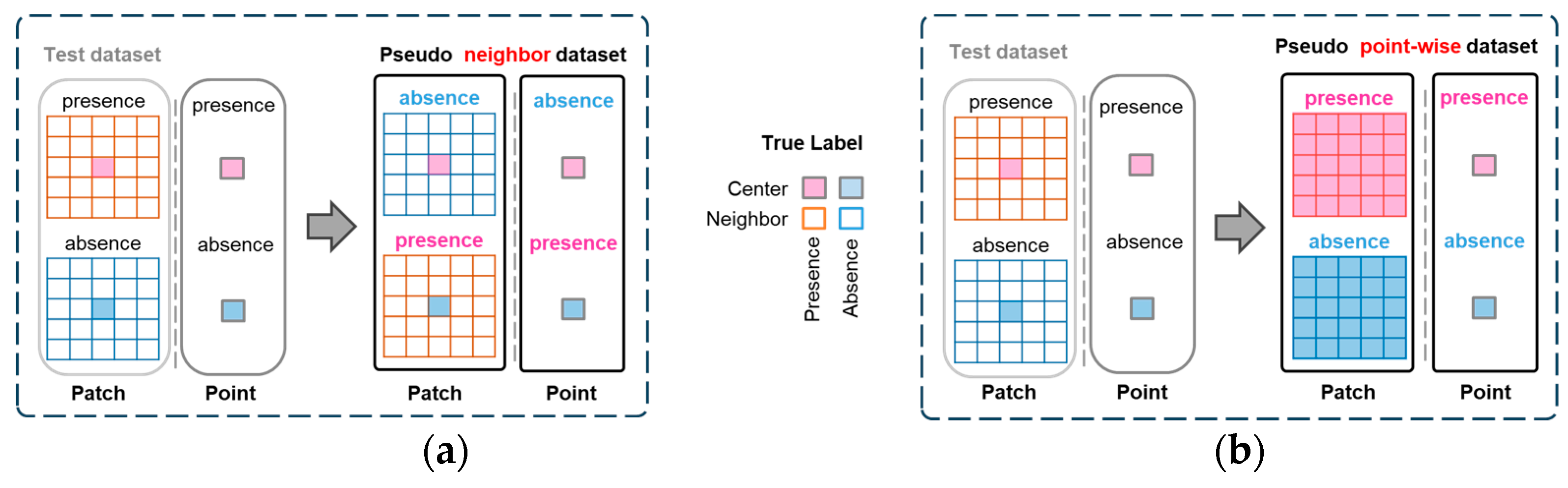
  • Robustness to Perturbed Data. The pseudo-neighbor and pseudo-point-wise tests confirmed the robustness of the proposed model. While the CNN model maintained high performance even with shuffled or point-restricted data, the Logistic Regression model’s accuracy dropped significantly, highlighting the advantage of patch-wise spatial modeling;
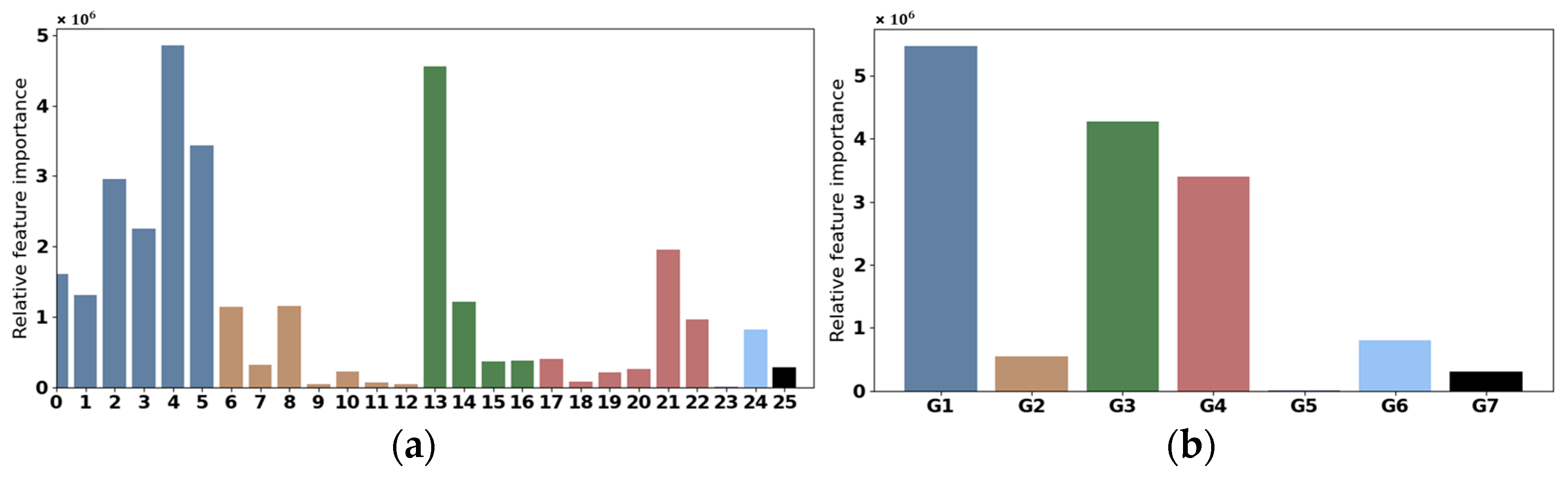
  • Feature Importance Analysis. The explainability analysis using Permutation Feature Importance (PFI) revealed that meteorological features such as precipitation, maximum temperature, and minimum temperature were the most influential factors in the model’s predictions. Interestingly, features like distance to roads showed lower importance, prompting further exploration into their ecological relevance.
The paper is organized as follows. Section 2 describes the data materials, including data collection and raw data processing. Section 3 introduces the proposed methods, including an overview of the model architecture and each component. Section 4 outlines the evaluation metrics and presents the experimental results, covering model development and performance, pseudo neighbor testing, pseudo point-wise testing, and interpretable analysis. Section 5 provides a discussion of the findings, while Section 6 concludes the paper and outlines potential directions for future research.

2. Materials

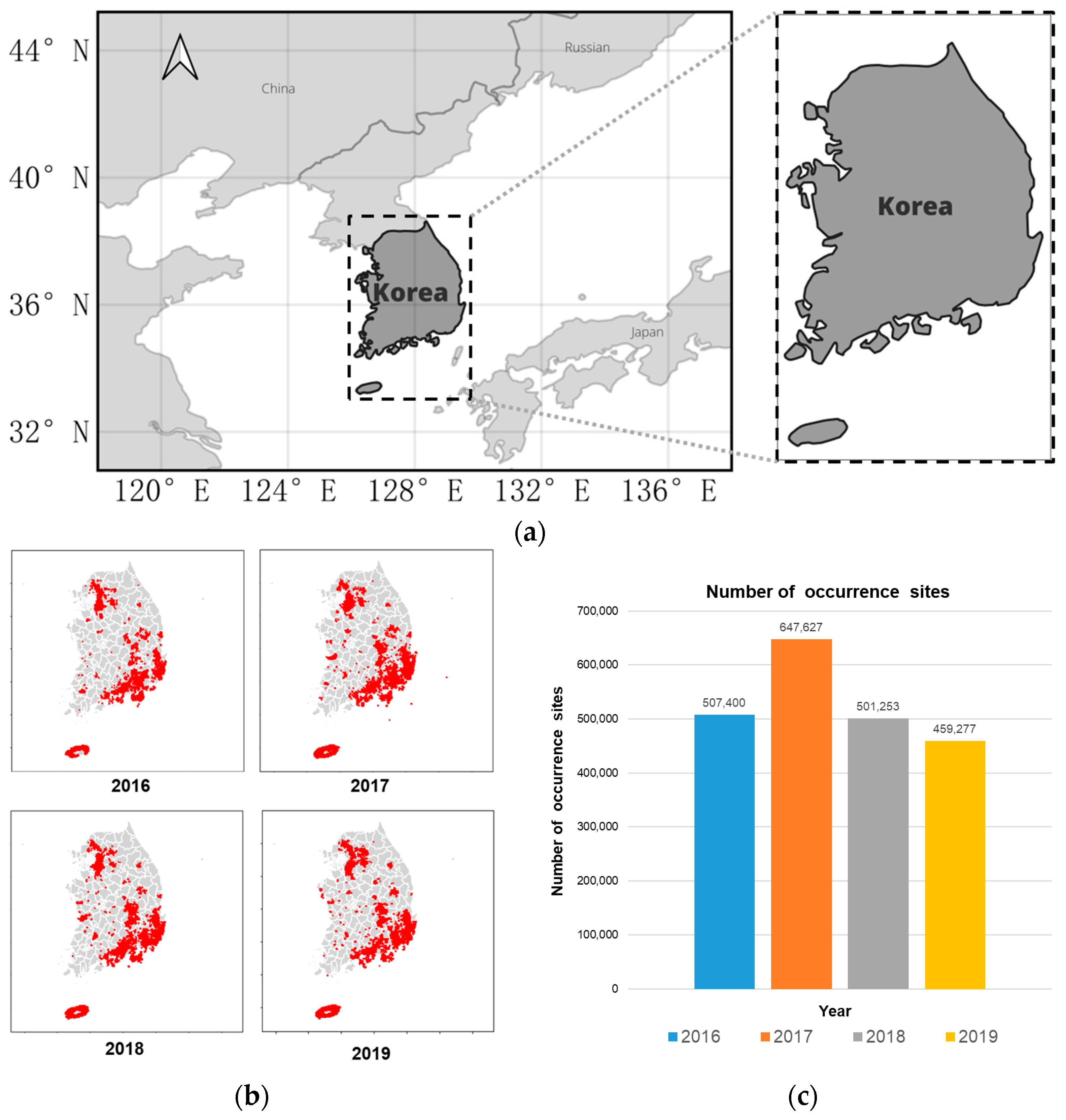
2.1. Data Collection

The area of interest in our research includes the whole of South Korea, as shown in Figure 2a. We primarily referred to the data collection methodology and structure outlined in work [7] to collect the data. Specifically, we obtained maps from the Forest Big Data Exchange Platform [19] that show the locations of PWD occurrences in South Korea from 2016 to 2019, like Figure 2b. The locations of occurrence for each year are not consistent; some locations are added or neglected through the years between 2016 and 2019 so that it is hard to directly apply the CA–Markov model. That is why the number of occurrences sites of each year from 2016 to 2019 are pretty different, as in Figure 2c, although PWD occurrence would be consistently increased.
The previous research [7] used seven environmental features, including geographical features (elevation, slope, and distance to roads) and meteorological features (annual mean temperature, minimum temperature in January, maximum temperature in July, and annual precipitation), to create datasets and models. In our study, we retained three geographical features and modified the meteorological features. As the peak activity period for Bursaphelenchus xylophilus (the causative agent of PWD) [1] spans from April to October, we used all the meteorological data (mean temperature, minimum temperature, maximum temperature, and precipitation) recorded during this period, instead of the four features mentioned above. We obtained this environmental feature data from the period 2016 to 2019, with a spatial resolution of 30 m by 30 m and raster dimensions of 17,511 by 20,362 pixels, as shown in Table 1. Figure 3 illustrates examples of environmental features. Figure 3a shows the maps of selected geographical features and the distribution of the “DistoRoad,” “Elevation,” and “Slope” features, with scale bars. Figure 3b also represents the maps of several meteorological features, the distribution of precipitation, mean temperature, maximum temperature, and minimum temperature for each month from April to October, with scale bars. Elevation and slope data were sourced from the National Geographic Information Institute of Korea [20]. The distance to roads refers to the proximity to public roads, calculated by integrating road data from the National Spatial Data Infrastructure Portal [21] and the Intelligent Transport Systems of Standard Node Link [22]. Meteorological data were collected from the Climate Information Portal of the Korea Meteorological Administration [23].
The PWD occurrence data are in shapefile format, a geospatial vector data format used by geographic information system (GIS) software. The environmental feature data are in Tagged Image File Format (TIFF), a format for storing raster graphics. We manage our data using open-source geographic information system software (QGIS, version 3.28.9), with the coordinate reference system set to Korea 2000/Central Belt 2010 (EPSG 5186).

2.2. Raw Data Processing

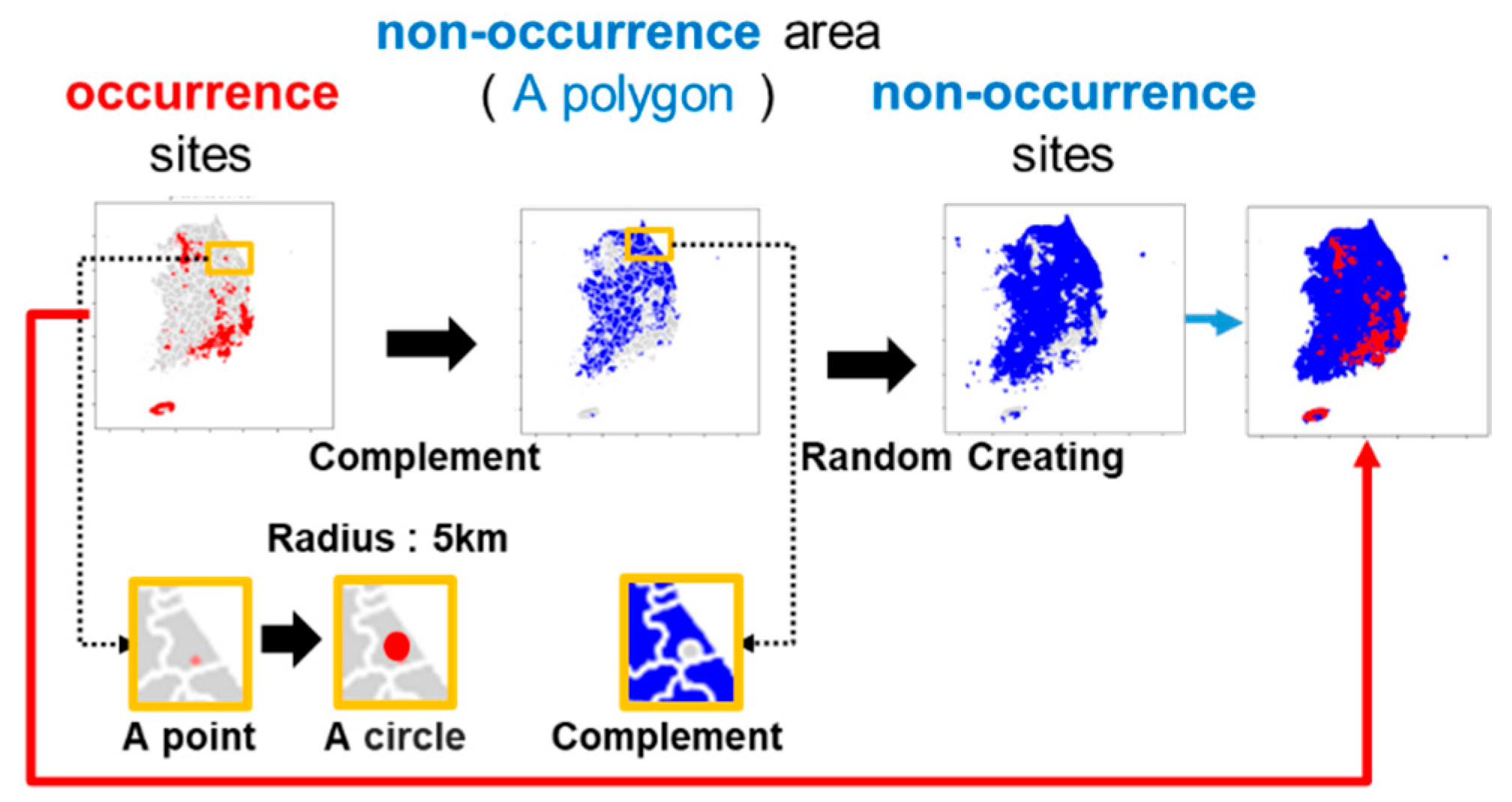
2.2.1. Non-Occurrence Site Generation

In this study, our task is a binary classification problem. As the positive samples are the occurrence sites, negative samples are necessary for data training. The “non-occurrence sites” are generated using the occurrence sites as references. Previous research [7] has noted that areas within 5 km of occurrence sites have relatively higher occurrence probabilities. Building upon this observation, as shown in Figure 4, we generated “non-occurrence areas” located 5 km away from the occurrence sites, and an equal number of “non-occurrence sites” are randomly generated with very low relative occurrence probabilities similar to occurrence sites. The corresponding geographical and meteorological features are sampled using the coordinates of occurrence sites and the generated “non-occurrence sites”.

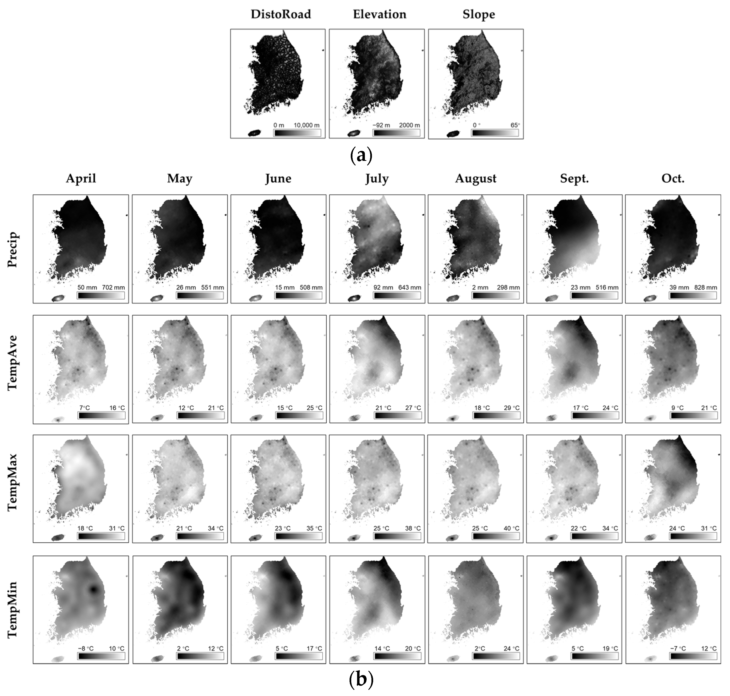
2.2.2. Features Selection

A recent study [7] conducted feature selection using the non-parametric Mann–Whitney U test [24] and the correlation coefficient between the features. In our study, we have a total of 31 types of features. As shown in Table 2, we only performed the non-parametric Mann–Whitney U test and did not calculate correlations, as this can be learned during deep learning model training. When performing the U test, if the sample size difference is large, the p-value magnitude also changes significantly. To align with the feature selection approach in [7], we matched the sample sizes (149 samples for occurrence sites, 149 samples for non-occurrence sites) during the U test by selecting sites with a minimum distance of 1 km between “non-occurrence sites” and a minimum distance of 5 km between occurrence sites.
As shown in Table 2, there is no significant difference between PWD occurrence and non-occurrence sites in maximum temperature in April, June, and September, precipitation in May, minimum temperature in June, and slope (p > 0.001). Other features, however, showed significant differences (p < 0.001). As [7] did, we removed all features with no significant difference, except for slope, leaving us with 26 features. We did not remove the slope because previous studies [25,26] have indicated a relationship between slope and PWD occurrence.

3. Methods

The overall architecture of our CNN model is shown in Figure 5. We primarily adopted a ResNet-style CNN for color image classification [18]. Specifically, instead of using a single row of tabular data with multiple feature cells as input for the point-wise model, we treated TIFF data in Figure 3 as a multi-channel geospatial image with a shape of (Height, Width, Channel), where each channel corresponds to a feature. Through the channel grouping block by performing an SE (Squeeze-and-excitation) operation [27] (sky blue block in Figure 5), we first obtained seven feature channels by a channel grouping module. The features were then downsampled through a 3 × 3 convolution layer to obtain an increase in the number of channels to 16 (yellow block in Figure 5), followed by feature extraction and classification using a widely-used Bottleneck block [18]; a CNN block further increased the number of channels to 64 (orange block in Figure 5). Finally, binary classification was performed using an average pooling layer and a fully-connected layer. The model was trained using cross-entropy loss (dark blue block in Figure 5). The following subsections describe the building blocks of overall architecture.

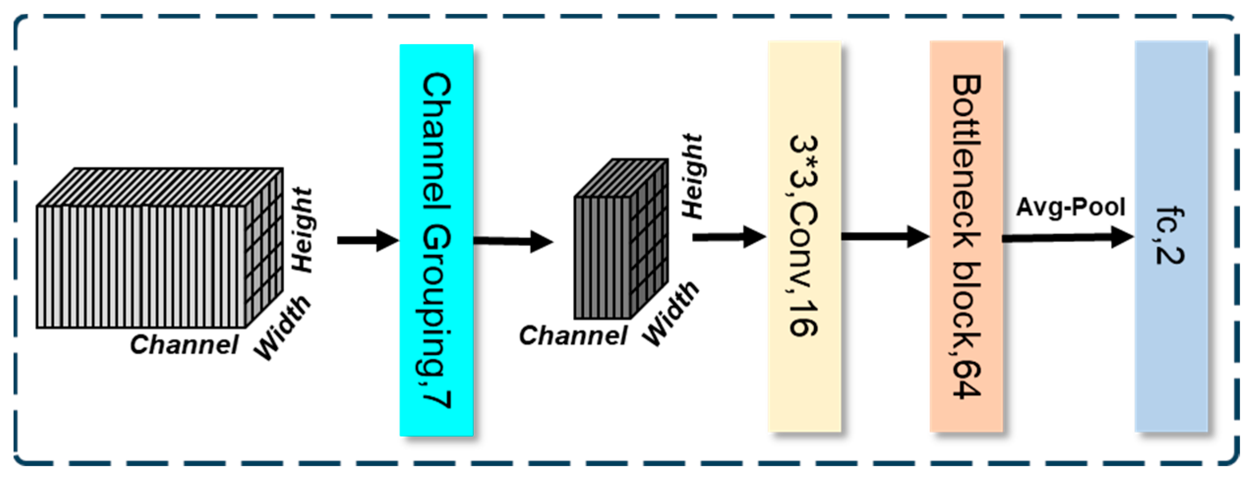
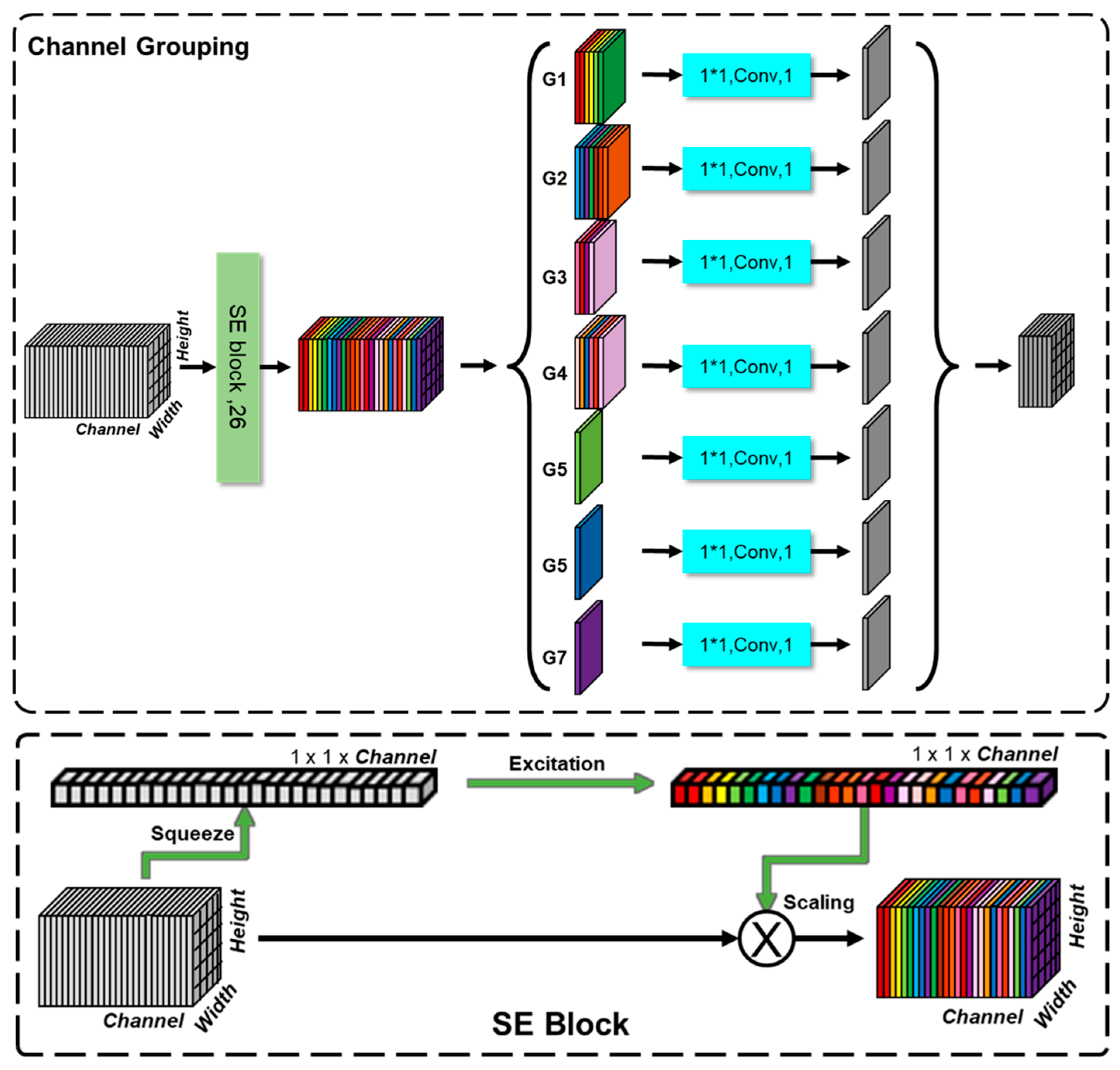
3.1. Channel Grouping

As mentioned in Section 2.2.2, in [7], for the meteorological features, based on their domain knowledge, they collected four types of feature data—annual mean temperature, minimum temperature in January, maximum temperature in July, and annual precipitation—and performed feature selection to train the model. In our study, we also collected four types of meteorological features every month, namely mean temperature, minimum temperature, maximum temperature, and precipitation.
However, unlike in [7], we did not manually select specific monthly features or approximate them into annual features by combining monthly data. Instead, we designed a channel grouping module, as shown in Figure 6.
Through this module, as shown in Table 3, we grouped the 23 meteorological feature channels processed in Section 2.2.2 into four channels, precipitation (Precip, G1), mean temperature (TempAve, G2), maximum temperature (TempMax, G3), and minimum temperature (TempMin, G4), using the SE block and a 1 × 1 convolution layer [28]. By training, the SE block, through the Squeeze and Excitation operation, automatically calculates the importance of each channel, as shown by the different colors in Figure 6, and assigns “weights” to them (scaling). These weights allow the model to adjust the importance of each feature during training. The meteorological feature channels are then combined with three other geographical feature channels, distance to road (DistoRoad, G5), elevation (Elevation, G6), and slope (Slope, G7), resulting in a total of seven grouped channels. Figure 7 shows an example of 1 × 1 convolution after SE block to obtain the TempAve (G2) channel group. In Figure 6, other branches of 1 × 1 convolution are similar to Figure 7 except the number of channels (features) to be aggregated.
By aggregating the feature channels into a few groups, the model can better explore the correlation between the feature channels, as we know the semantics of each channel. Using convolution layers, the model groups the 26 feature channels into seven final channels. This means that, during training on large data, the channel grouping module can adjust the “weights” or “bias” of specific months, helping to improve the model’s performance in predicting PWD occurrence and non-occurrence.

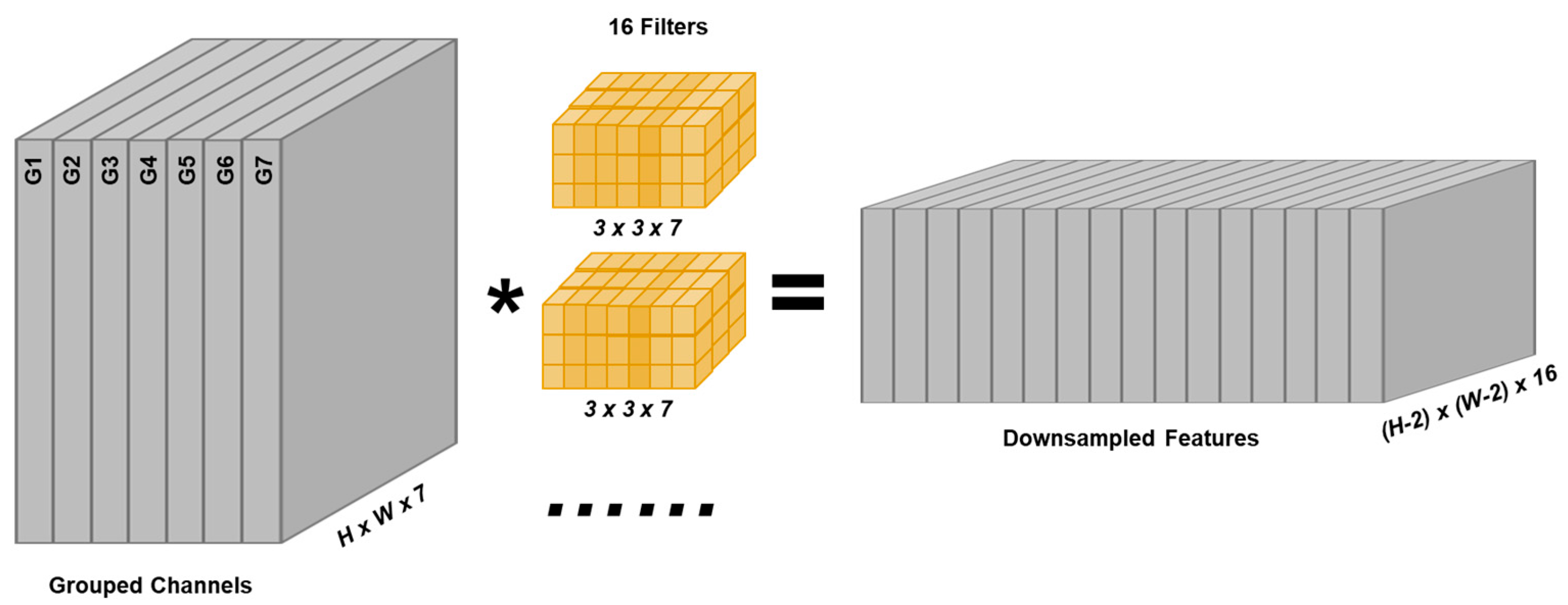
3.2. Downsampling with Increasing Number of Channels

In the ResNet [18] architecture, there are typically several convolutional layers at the head, referred to as the “stem.” Their primary function is to perform initial feature extraction and downsampling on the input, providing more compact and representative features for subsequent deeper network modules. In our method, we also performed downsampling after channel grouping, as in Figure 8. However, compared to the original ResNet, since our input has a relatively low resolution unlike the image classifiers [18], we used only a single convolutional layer with 16 filters of size 3 × 3. The shape of the features after downsampling is (H-2, W-2, 16).

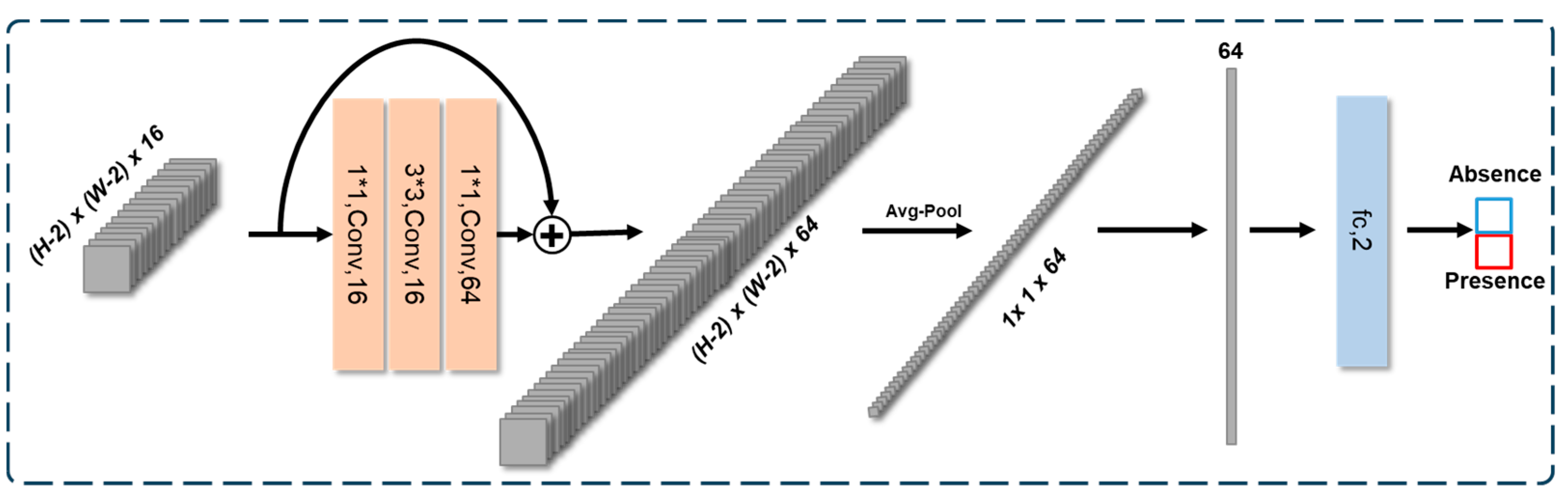
3.3. Bottleneck Block Upto FC (Fully Connected)-Based Classification Head

The basic modules in ResNet [18], each ResNet block, consists of two to three convolutional layers and incorporates a shortcut connection that directly adds the input to the output. By directly propagating the input signal, this structure includes a residual connection (skip connection), which mitigates information degradation between layers and thereby enhances the learning capability of deeper networks. This architecture facilitates easier training and enables the construction of deeper networks more effectively. In ResNet, the common types of blocks include the basic residual block and the bottleneck block. Although the bottleneck block employs 1 × 1 convolutions to reduce and then restore the number of channels, primarily to lower computational cost, and is generally designed for deeper networks, which may seem unsuitable for a shallow network like ours, we adopt the bottleneck block (orange block in Figure 9) in our method. This is because, in practice, 1 × 1 convolutions are also commonly used to capture complex channel-wise relationships [28], similar to their role in the previously introduced Channel Grouping block. Therefore, during this stage of feature extraction, the model can be regarded as performing a form of implicit Channel Grouping without any prior knowledge introduced by us. The shape of the features after the bottleneck block is (H-2, W-2, 64). Following the conventional approach of CNN classification models [18], an average pooling layer and a fully connected (FC) layer are applied for classification. The softmax output of the FC layer produces the probability of occurrence(presence) and non-occurrence(absence).

4. Experimental Results

The validity of the proposed method is demonstrated through several experiments. First, we implemented the model presented in Section 3 and compared it with a baseline point-wise prediction model based on Logistic Regression [29]. To analyze the differences between the two models, we conducted supplementary experiments, named Pseudo Neighbor Test and Pseudo Point-wise Test. Finally, we mentioned the interpretable analysis that reveals the feature importance of our CNN model. This section starts with evaluation metrics for measuring the performance of experimental results associated with those analyses.

4.1. Evaluation Metrics

We employed the f1-score, a version of the F-score [30], to evaluate the model’s performance. The F-score is a metric used to evaluate the predictive performance of a model. It is derived from two key components: precision and recall. Precision is the proportion of true positive results among all the instances predicted as positive, including both correct and incorrect predictions. Recall, on the other hand, is the proportion of true positive results among all the actual positive instances that should have been predicted. Precision and recall are then defined as Formulas (1) and (2). T P , F P , and F N are the numbers of true positives, false positives, and false negatives.
P r e c i s i o n = T P T P + F P
R e c a l l = T P T P + F N
The f1-score is calculated as the harmonic mean of precision and recall, providing a balanced measure that equally emphasizes both aspects within a single metric as the following formula:
F 1 = 2 r e c a l l 1 + p r e c i s i o n 1
For the comprehensive evaluation, we also employed accuracy, an intuitive metric that calculates the ratio of correct predictions to the total number of predictions made by the model, as shown in the following formula:
A c c u r a c y = T P + T N T P + F P + F N + T N

4.2. Experiments

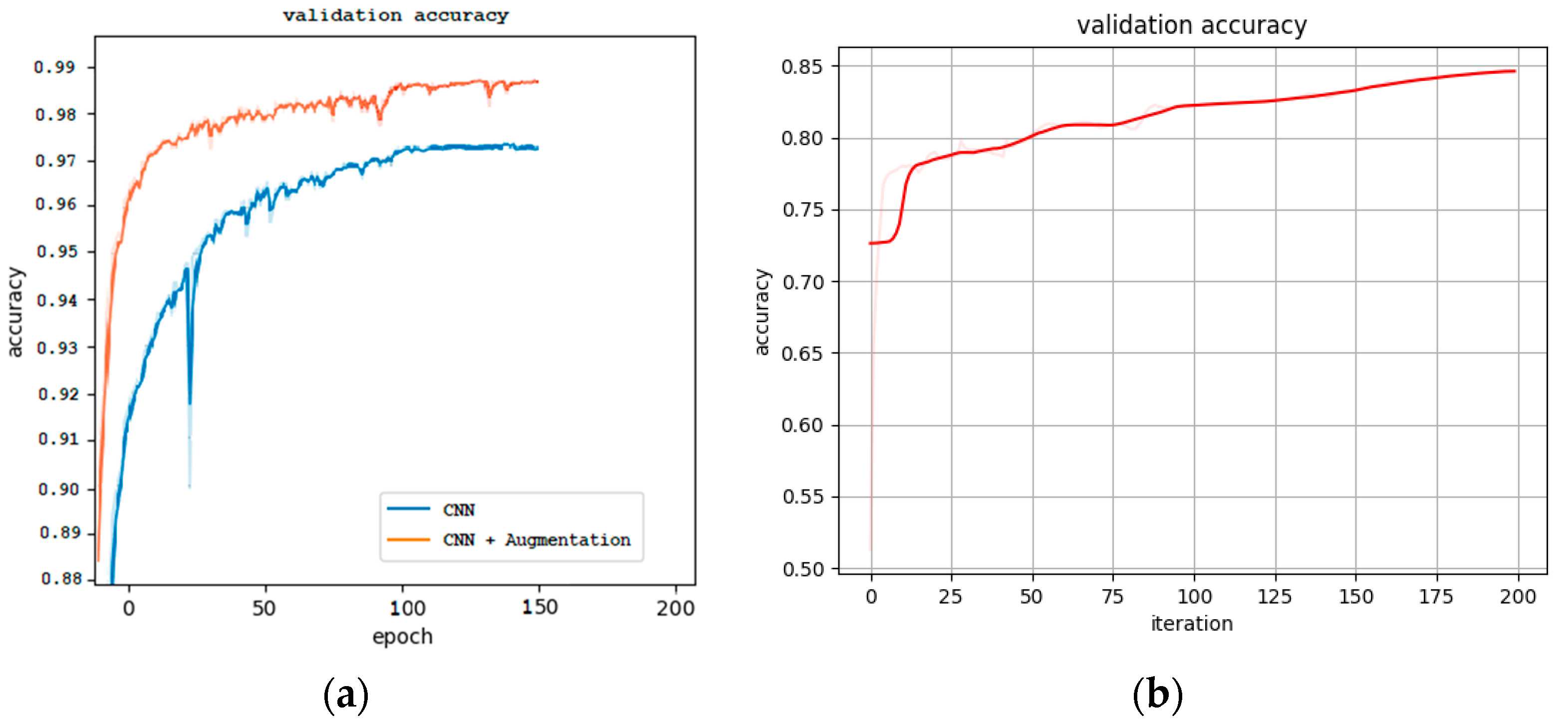
4.2.1. Model Development and Performance

After processing in Section 2.2, except for the maximum temperature in April, June, and September, precipitation in May, and minimum temperature in June, we have an equal number of occurrence and non-occurrence sample data, which include all the geographical features (elevation, slope, and distance to road) and meteorological features (mean temperature, minimum temperature, maximum temperature, and precipitation) recorded from April to October between 2016 and 2019. As shown in Table 4, we split the data into training, validation, and testing datasets for each year and later mixed them across years. The dataset is split into approximately 70% training, 20% validation, and 10% testing. The number of occurrence samples differs from the number of occurrence sites presented in Section 2.1, as multiple occurrence sites can be associated with the same single location (30 m by 30 m).
For CNN training, as illustrated in the patch-wise prediction in Figure 5, the patch-version samples are multichannel geospatial images with a patch size of 5 by 5 (150 m by 150 m) and 26 feature channels. We augmented the training dataset by taking 90°, 180°, and 270° rotations and horizontal and vertical flips, as these transformations would not alter the occurrence probabilities. For Logistic Regression model training, as shown in the point-wise prediction in Figure 1, the point-version samples are rows in the tabular data with 26-dimensional feature vectors. Note that the point-version samples are the central values of the corresponding patch-version samples.
We describe this dataset construction here rather than in Section 2, the Materials section, as it is integral to model development. This process, including data augmentation, directly contributes to subsequent model training and validation.
For the CNN model, we followed the default training settings provided by the MMPreTrain [31] toolkit, version 1.1.0. The CNN model was trained with the Adam optimizer [32], with a learning rate set to 0.001. For Logistic Regression, we followed the default training settings provided by Scikit-learn tools [33], version 1.2.2. Other hyperparameters are consistent with the toolkit defaults. The GPU RTX 3090 Ti was used for computation.
The classification results of different models are summarized in Table 5. Based on Table 5, comparing the point-wise prediction with the patch-wise prediction (without data augmentation), the patch-wise prediction achieved approximately a 9.7% higher F1-score than the point-wise prediction. This illustrates the validity of the proposed method, as the datasets are the same. Moreover, training with augmented data improved the F1-score by about 1% to 98.45%, Figure 10 showed the validation of CNN model and Logistic Regression model. The number of FLOPs (Floating-point Operations) per sample and parameters are also given in Table 5. Although the patch-wise CNN model is larger than the point-wise Logistic Regression model, its computational cost actually qualifies it as a tiny model. For comparison, MobileNetV2 [34], a lightweight CNN for real-time use on mobile devices, has 3.4 million parameters and 300 million FLOPs. To fairly analyze the baseline point-wise Logistic Regression and proposed patch-wise CNN model, we also conducted Pseudo neighbor testing and Pseudo Point-wise Testing using the CNN model without data augmentation.

4.2.2. Pseudo Neighbor Testing

As mentioned in Section 1, we assumed the occurrence of PWD at a specific location is not determined solely by its inherent features. Supposedly, it is also profoundly affected by the environmental conditions of the surrounding area. To test whether the proposed model is robust against disturbances to the center location, we prepared a pseudo neighbor dataset, as shown in Figure 11a.
For the whole test dataset prepared for measuring the performance of the CNN model, we randomly swapped the meteorological values of the surrounding locations between occurrence samples and non-occurrence samples and changed the labels following the label of surrounding locations. In Figure 11a, note that the “absence” (“presence”) pseudo test sample has blue (brown) meteorological surrounding features for the original “absence” (“presence”) sample but the features at the center location are preserved. In order to ensure the “pseudo” sites closely resemble ‘real’ sites in the world, we did not swap the geographical features. This implies the context meteorological features of all neighboring locations except the center location are changed with its label for testing the CNN model. If the prediction results depend on the context meteorological features of neighboring locations more than the center location, then it would well follow the changed labels of the neighboring locations. For point-wise Logistic Regression, only the labels of center location were changed without swapping the context meteorological features. Actually, the prediction results of point-wise Logistic Regression do not depend on the neighboring locations. In simpler terms, this can be likened to a scenario where a cat with a dog’s nose should still be identified as a cat by a model that takes the whole body into account; however, a model focusing solely on the nose might produce an incorrect classification.
If the patch-wise CNN model after training considers not only the center location but also the surrounding area (neighbors), the performance on this pseudo neighbor test dataset should not be abruptly decreased. On the other hand, the performance of the baseline model, which only considers the “center location,” should be relatively poor, because the ground truth has been changed and there is no way to consider the surrounding features. The results of this pseudo neighbor testing are summarized in Table 6. Compared with Table 5, the performance gap for the CNN model was not as severe as the amount of 7.56% in the F1-score, because at least the context meteorological features of neighboring locations were well coincided with the changed label. However, the baseline model performed poorly, exhibiting a substantial performance gap of 65.28% in the F1-score. This is due to the point-wise model’s inability to leverage the altered contextual meteorological information.

4.2.3. Pseudo Point-Wise Testing

The proposed CNN model considers both the central location and its neighboring areas, capturing the spatial dependencies necessary for accurate predictions. However, a critical question remains: can the proposed model still function effectively when only data from a specific location (point) are available, without any information about its neighbors?
To investigate this, we prepared a pseudo point-wise dataset, as illustrated in Figure 11b. We generated this dataset by replicating all the meteorological and geographical feature values of the specific location across its neighboring areas. This approach allowed us to simulate a point-wise scenario and evaluate the model’s ability to make predictions without real neighboring information. The results of this experiment are summarized in Table 7. Despite the lack of real neighboring data, the proposed model demonstrated robust performance. Specifically, the Logistic Regression model achieved the same F1-score of 87.69% in Table 5 when using the same point-wise dataset. Similarly, the CNN model, trained on the pseudo point-wise dataset, achieved superior performance with an F1-score of 97.31%. These findings indicate that the proposed model is still effective, even in scenarios where only point-specific data are available. Notably, the performance gap for the CNN model was just 0.1% in F1-score compared to Table 5, as we replicated the center feature values across neighboring points, which likely increased the probability of occurrence or non-occurrence.

4.3. Interpretable Analysis

In this section, we aim to interpret the feature importance in the model’s decision-making process using Permutation Feature Importance (PFI) [35]. PFI is a widely used technique that quantifies the importance of a feature by measuring the increase in the model’s prediction error after permuting the feature values. The underlying principle is straightforward: a feature is deemed “important” if shuffling its values significantly increases the prediction error, as this indicates that the model heavily relies on the feature for making accurate predictions. Conversely, a feature is considered “unimportant” if permuting its values results in little to no change in prediction error, suggesting that the feature contributes minimally or not at all to the model’s decision process. We used the Captum [36] toolkit (version 0.7.0), a model interpretability and understanding library for PyTorch, to apply PFI to our model and features.
Interpretable analyses were applied to the entire test dataset (74,564 samples for both presence and absence). PFI was applied at two levels: individual channels (features) and channel groups (feature groups). Figure 12 shows the sum of absolute PFI values for each channel and channel group. Here, higher PFI values correspond to greater importance in the model’s decision-making process. As shown in Table 3, both Figure 12a,b indicate that the most important feature groups tend to be G1 (“Precip”), G3 (“TempMax”), and G4 (“TempMin”). Notably, the feature channels in G1 are generally more important than most other feature channels, as shown in Figure 12a. However, an unexpected result was that G5 (“DistoRoad”) has relatively low importance. In Figure 12a, Precipitation in September (ID 4), Mean Temperature in June (ID 8), Maximum Temperature in May (ID 13), and Minimum Temperature in September (ID 21) emerge as the top feature channels. Mean Temperature in April (ID 6) and Mean Temperature in June (ID 8) exhibit similar levels of importance. Precipitation in September (ID 4) and Maximum Temperature in May (ID 13) are identified as the most important feature channels.

5. Discussion

The experiments and interpretability analysis highlight the effectiveness and robustness of the proposed patch-wise CNN model for predicting PWD occurrence. Compared to the point-wise Logistic Regression baseline, the CNN model significantly improved prediction accuracy by incorporating spatial dependencies, as evidenced by a 9.7% higher F1-score. Data augmentation further enhanced the model’s performance, contributing an additional 1% improvement. The pseudo-neighbor test demonstrated that the CNN effectively integrates information from surrounding areas, maintaining high accuracy despite perturbations in central location data. Similarly, the pseudo-point-wise test revealed the model’s adaptability, achieving robust predictions even with single-location inputs, outperforming the baseline.
The interpretable analysis, using PFI, provided insights into the model’s decision-making process. Features such as precipitation, maximum temperature, and minimum temperature were identified as most influential, particularly precipitation in September and maximum temperature in May. Surprisingly, features like the distance to roads showed limited importance in our study.
Overall, the proposed approach successfully addresses limitations of traditional point-wise models by leveraging spatial context and offering interpretability, paving the way for future improvements, such as exploring optimal patch sizes for enhanced predictive performance.
As we mentioned in the introduction, although the Logistic Regression Model (aka MaxEnt) [8] serves as our baseline, it is not the only point-wise model; studies such as [7,8,9,10] also follow point-wise modeling but differ in data composition. A study in the CA–Markov model [11], on the other hand, incorporates spatial dependencies similar to our approach but requires high-quality spatiotemporal PWD occurrence data on an appropriate scale. Due to data availability constraints, we could not comprehensively compare various models, which remain an important direction for future research. We hope this paper encourages further exploration and advancements in the research community of species distribution model (SDM) [37].
Once the PWD occurrence predictor is well-trained, it can be used to forecast PWD occurrences in future years, provided that the corresponding geographical and meteorological features can be accurately simulated using temporal prediction methods such as moving averages [38]. This presents a practical application for analyzing PWD spread and is another promising direction for future research.

6. Conclusions

In this study, we developed an interpretable prediction model for predicting the occurrence of PWD by incorporating both geographical and meteorological features. By utilizing a CNN that considers environmental data from surrounding areas (patch-wise) rather than individual points, we demonstrated a significant improvement in prediction accuracy compared to traditional point-wise models. Our model not only outperformed baseline models such as Logistic Regression but also incorporated XAI techniques to assess the importance of various features in the decision-making process.
We also evaluated the robustness of the model through various tests, including pseudo-neighbor and pseudo-point-wise testing, confirming that our model effectively captures spatial dependencies and performs well even with limited data. However, despite the promising results, the choice of patch size remains a crucial factor. Future research could focus on experimenting with different patch sizes to determine the optimal configuration that balances computational efficiency with predictive accuracy. Furthermore, since the adaptation of receptive fields in transformers is more flexible, transformer models with self-attention releasing locality constraints in convolution operation may be considerable in the future. This could further enhance the model’s performance and adaptability for large-scale environmental monitoring systems that require patch-wise SDM models [37].

Author Contributions

Conceptualization, W.W. and J.L.; methodology, W.W. and J.L.; software, W.W.; validation, W.W.; resource, J.L.; data curation, J.L.; writing—original draft preparation, W.W.; writing—review and editing, W.W. and J.L.; supervision, J.L.; project administration, J.L.; funding acquisition, J.L. All authors have read and agreed to the published version of the manuscript.

Funding

This research was funded by the National Research Foundation of Korea (NRF) under grant number RS-2024-00340948.

Data Availability Statement

The PWD occurrence sites data were obtained from Forest Big Data Exchange Platform and are available from the URL https://www.bigdata-forest.kr/frn/index (accessed 30 November 2024) with the permission of Forest Big Data Exchange Platform; and other dataset used to support the findings of this study can be obtained from the corresponding author upon request.

Acknowledgments

We would like to express our sincere gratitude to Ridip Khanal for his significant contributions in software and writing—review and editing. His expertise and meticulous attention to detail have greatly enhanced the rigor and accuracy of this research. We deeply appreciate his dedication and support, which were instrumental in the successful completion of this study.

Conflicts of Interest

The authors declare that there is no conflict of interest.

References

  1. Khan, M.A.; Ahmed, L.; Mandal, P.K.; Smith, R.; Haque, M. Modelling the dynamics of Pine Wilt Disease with asymptomatic carriers and optimal control. Sci. Rep. 2020, 10, 11412. [Google Scholar] [CrossRef]
  2. Gent, D.H.; Schwartz, H.F. Validation of potato early blight disease forecast models for Colorado using various sources of meteorological data. Plant Dis. 2003, 87, 78–84. [Google Scholar] [CrossRef]
  3. Roubal, C.; Regis, S.; Nicot, P.C. Field models for the prediction of leaf infection and latent period of Fusicladium oleagineum on olive based on rain, temperature and relative humidity. Plant Pathol. 2013, 62, 657–666. [Google Scholar] [CrossRef]
  4. Valdez-Torres, J.B.; Soto-Landeros, F.; Osuna-Enciso, T.; Baez-Sanudo, M.A. Phenological prediction models for white corn (Zea mays L.) and fall armyworm (Spodoptera frugiperda J.E. Smith). Agrociencia 2012, 46, 399–410. [Google Scholar]
  5. Laderach, P.; Ramirez-Villegas, J.; Navarro-Racines, C.; Zelaya, C.; Martinez-Valle, A.; Jarvis, A. Climate change adaptation of coffee production in space and time. Clim. Chang. 2017, 141, 47–62. [Google Scholar] [CrossRef]
  6. Schwartz, M.W. Potential effects of global climate change on the biodiversity of plants. For. Chron. 1992, 68, 462–471. [Google Scholar] [CrossRef]
  7. Lee, D.-S.; Choi, W.I.; Nam, Y.; Park, Y.-S. Predicting potential occurrence of pine wilt disease based on environmental factors in South Korea using machine learning algorithms. Ecol. Inform. 2021, 64, 101378. [Google Scholar] [CrossRef]
  8. Hao, Z.; Fang, G.; Huang, W.; Ye, H.; Zhang, B.; Li, X. Risk prediction and variable analysis of pine wilt disease by a maximum entropy model. Forests 2022, 13, 342. [Google Scholar] [CrossRef]
  9. Yoon, S.; Jung, J.-M.; Hwang, J.; Park, Y.; Lee, W.-H. Ensemble evaluation of the spatial distribution of pine wilt disease mediated by insect vectors in South Korea. For. Ecol. Manag. 2023, 529, 120677. [Google Scholar] [CrossRef]
  10. Jung, J.-M.; Yoon, S.; Hwang, J.; Park, Y.; Lee, W.-H. Analysis of the spread distance of pine wilt disease based on a high volume of spatiotemporal data recording of infected trees. For. Ecol. Manag. 2024, 553, 121612. [Google Scholar] [CrossRef]
  11. Liu, D.; Zhang, X. Occurrence Prediction of Pine Wilt Disease Based on CA–Markov Model. Forests 2022, 13, 1736. [Google Scholar] [CrossRef]
  12. Zhang, B.; Ye, H.; Lu, W.; Huang, W.; Wu, B.; Hao, Z.; Sun, H. A Spatiotemporal Change Detection Method for Monitoring Pine Wilt Disease in a Complex Landscape Using High-Resolution Remote Sensing Imagery. Remote Sens. 2021, 13, 2083. [Google Scholar] [CrossRef]
  13. Deng, X.; Tong, Z.; Lan, Y.; Huang, Z. Detection and Location of Dead Trees with Pine Wilt Disease Based on Deep Learning and UAV Remote Sensing. AgriEngineering 2020, 2, 294–307. [Google Scholar] [CrossRef]
  14. Thapa, N.; Khanal, R.; Bhattarai, B.; Lee, J. Pine Wilt Disease Segmentation with Deep Metric Learning Species Classification for Early-Stage Disease and Potential False Positive Identification. Electronics 2024, 13, 1951. [Google Scholar] [CrossRef]
  15. Kosarevych, R.; Jonek-Kowalska, I.; Rusyn, B.; Sachenko, A.; Lutsyk, O. Analysing Pine Disease Spread Using Random Point Process by Remote Sensing of a Forest Stand. Remote Sens. 2023, 15, 3941. [Google Scholar] [CrossRef]
  16. Mathew, A.; Amudha, P.; Sivakumari, S. Deep learning techniques: An overview. Adv. Mach. Learn. Technol. Appl. Proc. AMLTA 2021, 2020, 599–608. [Google Scholar]
  17. Krizhevsky, A.; Sutskever, I.; Hinton, G.E. Imagenet classification with deep convolutional neural networks. Commun. ACM 2017, 60, 84–90. [Google Scholar]
  18. He, K.; Zhang, X.; Ren, S.; Sun, J. Deep residual learning for image recognition. In Proceedings of the IEEE Conference on Computer Vision and Pattern Recognition, Las Vegas, NV, USA, 27–30 June 2016; pp. 770–778. [Google Scholar]
  19. Koren National Information Society Agency. 2019. Available online: https://www.bigdata-forest.kr/ (accessed on 27 March 2025).
  20. National Geographic Information Institute of Korea. 2019. Available online: https://www.ngii.go.kr/ (accessed on 27 March 2025).
  21. National Spatial Data Infrastructure Portal. 2023. Available online: https://www.vworld.kr/ (accessed on 27 March 2025).
  22. Intelligent Transport Systems of Standard Node Link. 2019. Available online: https://www.its.go.kr/nodelink/nodelinkRef (accessed on 27 March 2025).
  23. Climate Information Portal of the Korea Meteorological Administration. 2017. Available online: https://www.climate.go.kr/ (accessed on 27 March 2025).
  24. McKnight, P.E.; Najab, J. Mann-Whitney U Test. In The Corsini Encyclopedia of Psychology; John Wiley & Sons: Hoboken, NJ, USA, 2010; p. 1. [Google Scholar]
  25. Park, S.-G.; Hong, S.-H.; Oh, C.-J. A Study on Correlation Between the Growth of Korean Red Pine and Location Environment in Temple Forests in Jeollanam-do, Korea. Korean J. Environ. Ecol. 2017, 31, 409–419. [Google Scholar] [CrossRef]
  26. Lee, D.-S.; Nam, Y.; Choi, W.I.; Park, Y.-S. Environmental factors influencing on the occurrence of pine wilt disease in Korea. Korean J. Ecol. Environ. 2017, 50, 374–380. [Google Scholar] [CrossRef]
  27. Hu, J.; Shen, L.; Sun, G. Squeeze-and-excitation networks. In Proceedings of the IEEE Conference on Computer Vision and Pattern Recognition, Salt Lake City, UT, USA, 18–23 June 2018. [Google Scholar] [CrossRef]
  28. Szegedy, C.; Liu, W.; Jia, Y.; Sermanet, P.; Reed, S.; Anguelov, D.; Erhan, D.; Vanhoucke, V.; Rabinovich, A. Going deeper with convolutions. In Proceedings of the IEEE Conference on Computer Vision and Pattern Recognition, Boston, MA, USA, 7–12 June 2015; pp. 1–9. [Google Scholar] [CrossRef]
  29. LaValley, M.P. Logistic regression. Circulation 2008, 117, 2395–2399. [Google Scholar] [CrossRef]
  30. Goutte, C.; Eric, G. A Probabilistic Interpretation of Precision, Recall and F-Score, with Implication for Evaluation. European Conference on Information Retrieval; Springer: Berlin/Heidelberg, Germany, 2005. [Google Scholar]
  31. MMPreTrain Contributors. OpenMMLab’s Pre-training Toolbox and Benchmark. 2023. Available online: https://github.com/open-mmlab/mmpretrain (accessed on 27 March 2025).
  32. Kingma, D.P. Adam: A method for stochastic optimization. arXiv 2014, arXiv:1412.6980. [Google Scholar]
  33. Bisong, E.; Ekaba, B. Introduction to Scikit-learn. In Building Machine Learning and Deep Learning Models on Google Cloud Platform: A Comprehensive Guide for Beginners; Apress: Berkeley, CA, USA, 2019; pp. 215–229. [Google Scholar]
  34. Sandler, M.; Howard, A.; Zhu, M.; Zhmoginov, A.; Chen, L.C. Mobilenetv2: Inverted residuals and linear bottlenecks. In Proceedings of the IEEE Conference on Computer Vision and Pattern Recognition, Salt Lake City, UT, USA, 18–23 June 2018; pp. 4510–4520. [Google Scholar] [CrossRef]
  35. Altmann, A.; Toloşi, L.; Sander, O.; Lengauer, T. Permutation importance: A corrected feature importance measure. Bioinformatics 2010, 26, 1340–1347. [Google Scholar] [CrossRef] [PubMed]
  36. Kokhlikyan, N.; Miglani, V.; Martin, M.; Wang, E.; Alsallakh, B.; Reynolds, J.; Melnikov, A.; Kliushkina, N.; Araya, C.; Yan, S.; et al. Captum: A unified and generic model interpretability library for pytorch. arXiv 2020, arXiv:2009.07896. [Google Scholar]
  37. Farashi, A.; Mohammad, A.-N. Basic Introduction to Species Distribution Modelling. Ecosystem and Species Habitat Modeling for Conservation and Restoration; Springer Nature: Singapore, 2023; pp. 21–40. [Google Scholar] [CrossRef]
  38. Mulla, S.; Pande, C.B.; Singh, S.K. Times series forecasting of monthly rainfall using seasonal auto regressive integrated moving average with EXogenous variables (SARIMAX) model. Water Resour. Manag. 2024, 38, 1825–1846. [Google Scholar] [CrossRef]
Figure 1. Point-wise prediction and patch-wise prediction. Point-wise prediction considers only the local geographical and meteorological features, which may neglect spatial dependencies. In contrast, patch-wise prediction can incorporate the surrounding area’s context, capturing broader environmental factors that influence PWD occurrence.
Forests 16 00935 g001
Figure 2. PWD occurrence sites. (a) study area, indicated by the dark region within the dashed rectangle. (b) The actual occurrence area of PWD of each year from 2016 to 2019 within the study area. The “red area” indicates the PWD occurrence area. (c) The number of occurrences sites of each year from 2016 to 2019 within the study area.
Forests 16 00935 g002
Figure 3. Distribution of environmental features in 2016. (a) Geographical features, the distribution of the “DistoRoad,”” Elevation,” and “Slope” features, with scale bars. (b) Meteorological features, the distribution of precipitation, mean temperature, maximum temperature, and minimum temperature for each month from April to October, with scale bars.
Forests 16 00935 g003
Figure 4. Non-occurrence site generation. The “red area” indicates the PWD occurrence area, and the “blue area” indicates the PWD non-occurrence area. Non-occurrence sites were generated 5 km away from occurrence sites, with an equal number of randomly selected sites exhibiting very low relative occurrence probabilities. Geographical and meteorological features were extracted using the coordinates of both occurrence and non-occurrence sites.
Forests 16 00935 g004
Figure 5. Model Architecture. The model groups channels into 7 feature channels, downsampled through a convolution layer. Feature extraction is performed with a Bottleneck block, followed by binary classification using average pooling and a fully connected layer.
Forests 16 00935 g005
Figure 6. Channel Grouping. Meteorological feature channels were grouped to four (mean temperature, minimum temperature, maximum temperature, and precipitation) using the SE block and a 1 × 1 convolution layer, then combined with geographical features to form seven grouped channels.
Forests 16 00935 g006
Figure 7. An example of channel grouping for TempAve (G2). Here, seven features are automatically weighted as shown in different colors and aggregated 1 × 1 convolution in Figure 6 by training.
Forests 16 00935 g007
Figure 8. Structure of the downsampleing and increasing number of channels.
Forests 16 00935 g008
Figure 9. Structure of the bottleneck block upto FC-based classification head.
Forests 16 00935 g009
Figure 10. Validation accuracy of CNN model (a) and Logistic Regression model (b). The CNN training process with the augmented dataset showed better efficiency from the beginning, and the final accuracy was also higher compared to the non-augmented dataset.
Forests 16 00935 g010
Figure 11. Pseudo test datasets: (a) Pseudo neighbor dataset; the meteorological values of the central location were randomly swapped between occurrence and non-occurrence samples, with labels unchanged. (b) Pseudo point-wise dataset; the values from a specific location were replicated across neighboring areas to simulate a point-wise scenario.
Forests 16 00935 g011
Figure 12. PFI of input features: (a) Channels. ‘9_Precip’ (ID 4), ‘6_TempAve’ (ID 8), ‘5_TempMax’ (ID 13), and ‘9_TempMin’ (ID 21) are the top features, with ‘4_TempAve’ (ID 6) and ‘6_TempAve’ (ID 8) showing similar importance. (b) Channel Groups. The most important feature groups are G1 (‘Precip’), G3 (‘TempMax’), and G4 (‘TempMin’). Notably, features in G1 generally surpass others in importance.
Forests 16 00935 g012
Table 1. Description of environmental features. “Alias” refers to the feature name used in this paper. Months formatted as “4: April, 5: May, 6: June, 7: July, 8: August, 9: September, 10: October”, and “#(4~10)” indicates each month from April to October.
AliasFeatureUnit
DistoRoadDistance to roadMeter (m)
ElevationElevationMeter (m)
SlopeSlopeDegree (°)
#(4~10)_PrecipMonthly PrecipitationMillimeter (mm)
#(4~10)_TempAveMonthly Mean temperatureDegree Celsius (°C)
#(4~10)_TempMaxMonthly Maximum temperatureDegree Celsius (°C)
#(4~10)_TempMinMonthly Minimum temperatureDegree Celsius (°C)
Table 2. Statistical Differences in Features between PWD Occurrence and Non-Occurrence Sites (Mann–Whitney U test, p-value). (a) Geographical Features; (b) Meteorological Features. No significant differences were observed in maximum temperature (April, June, and September), precipitation (May), minimum temperature (June), and slope (p > 0.001; values in bold in the table). All other features exhibited significant differences (p < 0.001).
Featurep-value
DistoRoad<0.001
Elevation<0.001
Slope0.919
(a)
FeatureAprilMayJuneJulyAugustSept.Oct.
Precip<0.0010.067<0.001<0.001<0.001<0.001<0.001
TempAve<0.001<0.001<0.001<0.001<0.001<0.001<0.001
TempMax0.833<0.0010.031<0.001<0.0010.414<0.001
TempMin<0.001<0.0010.119<0.001<0.001<0.001<0.001
(b)
Table 3. Feature groups and their corresponding features.
Group IDGroup NameFeature ID List 1
G1Precip0:4_Precip 1:6_Precip2:7_Precip3:8_Precip4:9_Precip5:10_Precip
G2TempAve6:4_TempAve7:5_TempAve8:6_TempAve9:7_TempAve10:8_TempAve11:9_TempAve12:10_TempAve
G3TempMax 13:5_TempMax 14:7_TempMax15:8_TempMax 16:10_TempMax
G4TempMin17:4_TempMin18:5_TempMin 19:7_TempMin20:8_TempMin21:9_TempMin22:10_TempMin
G5DistoRoad 23:DistoRoad
G6Elevation 24:Elevation
G7Slope 25:Slope
1 Feature ID: Feature Alias.
Table 4. Dataset Division. The split ratios are approximately 7:2:1. Only the training dataset was augmented using five different methods for CNN training.
DatasetLabelTrainValTestTotal
2016Presence122,35434,91117,362174,627
Absence122,35434,91117,362174,627
2017Presence175,31550,12425,055250,494
Absence175,31550,12425,055250,494
2018Presence138,21739,20819,725197,150
Absence138,21739,20819,725197,150
2019Presence86,05724,88412,422123,363
Absence86,05724,88412,422123,363
(Augmented)
Dataset
Presence6 × 521,943149,12774,5643,355,349
Absence6 × 521,943149,12774,5643,355,349
Table 5. Comparison of performance of patch-wise model and point-wise model. Bold values indicate the highest performance.
ModelDataset TypePrecisionRecallF1-ScoreAcc. 3#FLOPs#Params.
LR 1Point-wise87.7287.6587.6987.690.056 K0.027 K
CNNPatch-wise97.4197.4197.4197.4156.057 K6.571 k
CNN (+Aug. 2)Patch-wise98.4598.4598.4598.4556.057 K6.571 k
1 Logistic Regression 2 Augmentation 3 Accuracy.
Table 6. The results of pseudo neighbor testing. Bold values indicate the highest performance.
ModelDataset TypePrecisionRecallF1-ScoreAcc. 1
Logistic RegressionPoint-wise23.2021.6622.4124.98
CNNPatch-wise90.7489.9089.8589.90
1 Accuracy.
Table 7. The results of pseudo point-wise testing. Bold values indicate the highest performance.
ModelDataset TypePrecisionRecallF1-ScoreAcc. 1
Logistic RegressionPoint-wise87.7287.6587.6987.69
CNNPatch-wise97.3197.3197.3197.31
1 Accuracy.
Disclaimer/Publisher’s Note: The statements, opinions and data contained in all publications are solely those of the individual author(s) and contributor(s) and not of MDPI and/or the editor(s). MDPI and/or the editor(s) disclaim responsibility for any injury to people or property resulting from any ideas, methods, instructions or products referred to in the content.

