Floristic vs. Dominant Classification Approaches Applied to Geospatial Modeling of Mixed and Broadleaf Forest Types in the Northwestern Caucasus (Russia)

Abstract

The Caucasus Mountains are recognized as a global center of biodiversity but currently face significant risks of degradation due to intensified economic development and the effects of climate change. Forest inventory and mapping are essential for biodiversity conservation in the Caucasus region. Geospatial modeling is a common method of thematic mapping, but its reliability depends heavily on the initial classification of reference data used for model training. Modern vegetation science features various classification approaches, most of which were developed independently of digital mapping practices and are rarely assessed for their suitability in geospatial modeling. To fill this gap, we classified the same dataset of vegetation relevés from mixed and broadleaf forests in the northwestern Caucasus using two approaches, based on floristic and dominant concepts, and compared the predictive performance of geospatial models trained on these datasets. We considered multiple types of geospatial variables, including optical satellite imagery, a digital elevation model (DEM), and bioclimatic and soil features, to evaluate their informativeness for spatial differentiation of the resulting forest types and to identify optimal variable combinations for modeling via multistage feature selection. We trained several models using different variable sets and machine learning methods for both classifications and evaluated their accuracy via nested cross-validation. The forest types produced by the two approaches scarcely matched, and the selected variable sets for model training differed accordingly. Unexpectedly, bioclimatic and soil variables were more effective than DEM- and satellite-derived variables, despite their coarser spatial resolution. Floristic-based geospatial models outperformed dominant-based models in terms of forest-type separability and predictive accuracy. Therefore, a floristic classification approach may be preferable for forests with complex species composition, both ecologically and in terms of the reliability of geospatial modeling and the derived mapping results.

1. Introduction

The Caucasus Mountains represent a global center of biodiversity, with flora and fauna rich in endemic taxa [1]. Forests preserve a substantial proportion of this species diversity, providing habitats for world-protected large mammals, such as the leopard (Panthera pardus L.), the Caucasian forest cat (Felis lybica (silvestris) caucasica Satunin), and the European bison (Bison bonasus L.), as well as various relict plants, such as yew (Taxus baccata L.). Highly productive mixed coniferous–broadleaf forests of the North Caucasus also play a significant role in carbon sequestration across the Russian Federation [2]. Due to orographic and climatic factors, almost two-thirds of these forests are located in the northwestern part of the mountains, west of Mount Elbrus, Europe’s highest peak. Biodiversity in the Caucasus is currently threatened by intensified, and often unregulated, economic development [3] and the effects of climate change [4,5]. Effective biodiversity conservation in the region requires comprehensive forest and ecosystem inventories that enable systematic organization and reliable representation of relevant information.

Vegetation mapping is an important tool for inventorying habitats and assessing biodiversity [6]. Geospatial modeling, combining remote sensing data and machine learning, is a common method for thematic vegetation mapping, offering consistent large-scale results with relatively low labor and time investment [7,8]. The realism of geospatial models and the informativeness of derivative maps depend strongly on the researcher’s initial perception of vegetation diversity in the reference data used for model training, i.e., on the thematic classification of phytocoenoses [9,10]. Modern vegetation science features various classification approaches, most of which were originally developed independently of contemporary digital mapping practices. Therefore, any approach must be evaluated for suitability and limitations before application in mapping tasks.

Historically, the dominant approach, which groups phytocoenoses based on the high abundance of particular species, was the first to be developed. Various dominance-based classification systems have since been proposed. For example, a basic implementation considers one or several dominant species in the uppermost phytocoenose layer [11]. Other commonly used variants consider dominant species (plants or lichens) in each vegetation layer [12], together with the dominant plant life forms and phytocoenose topographic localization [13]. Many of these classifications were developed intuitively, particularly for polydominant phytocoenoses, without formalized rules, limiting comparability and unified implementation. Consequently, dominant-based classifications have been criticized, and alternative approaches have been proposed [14].

The floristic (or ecological–floristic) approach, proposed by J. Braun-Blanquet [15], recognizes vegetation types based on floristic composition, i.e., on a more or less broad set of plant (and often lichen) taxa, of species or intra-species rank. Within this approach, the presence of particular taxa combinations is considered an important diagnostic feature for classification units, referred to as ‘syntaxon’, and the classification system itself is termed ‘syntaxonomy’ [14,16,17].

Different classification approaches, even when applied to the same dataset, can produce class sets that differ substantially in both semantics and elemental composition. The degree of discrepancy depends on the depth of methodological differences and the species composition of the communities analyzed. In a large-scale study, Costanza et al. [18] compared three different classification systems—dominant, floristic, and data-driven unsupervised—using over 117,000 forest inventory plots across the United States. They found that only 20% of classes had one-to-one analogs across systems, and these well-matched forest types were characterized mainly by narrow ecological niches and low diversity in tree species composition.

Large differences between floristic and dominant classifications alone do not make one approach more correct or reliable. The choice between them depends on the specific research objectives and intended applications. The dominant approach provides an intuitive, relatively universal, and easy-to-implement framework for classifying forest ecosystems, especially when only top-layer tree species are considered, which explains its widespread use in remote sensing-based forest mapping [19,20,21,22,23]. However, when forest stands consist of multiple species without clear dominants, such classifications become more formal than substantial and offer limited value for spatial differentiation of natural forest types [24,25]. Conversely, floristic classification is better suited to characterizing forests with complex species composition and is widely used in biodiversity conservation tasks [26,27,28], although it typically requires more sophisticated and case-specific implementation. Despite these well-known distinctions, studies directly comparing the performance of the two approaches in geospatial modeling and forest-type mapping using the same reference data for a specific area remain extremely rare.

Therefore, the core aim of our study was to compare a complex, expertise-based floristic approach with a simple, formalized dominant approach regarding their ability to produce clearly distinguishable classes for geospatial modeling-based forest mapping under the same data conditions. Specifically, our primary objective was to obtain two independent classification results for a single dataset of field plots and to evaluate the predictive performance of models trained on both classification variants using a set of relevant geospatial variables. The polydominant species composition of the broadleaf and mixed forests of the northwestern Caucasus make this region an appropriate reference for such a comparison, given the expected discrepancies between classifications and the potential challenges of differentiating complex forest types through modeling. Previous studies in the North Caucasus have primarily focused on local mapping of coniferous and mixed coniferous–deciduous forests [29] or individual coniferous species such as fir (Abies nordmanniana (Stev.) Spach), spruce (Picea orientalis (L.) Link) [30], and pine (Pinus sylvestris L.) [31]. These studies naturally adopt the dominant approach, as relatively pure samples of selected tree species are used for geospatial model training, and resulting forest types are constructed from independently predicted species probabilities. Other studies have used the well-known MaxEnt framework [32] to model potential habitats (ecological niches) for selected tree species [33,34,35] and forest communities [36]. However, such results represent potential rather than actual spatial distributions and offer limited interpretability regarding the reliability of spatial discrimination among forest types.

The secondary study objectives were as follows:

• To evaluate the similarity or dissimilarity between the dominant and floristic classifications;
• To perform feature selection from available geospatial variables of different types and origins for model training, and to compare the selection results for both classification variants;
• To test several machine learning algorithms with different optimized variable sets for both classification variants.

These evaluations are necessary to understand how the choice of classification method influences the entire geospatial modeling pipeline and to identify optimal combinations of variables and machine learning algorithms. The results will indicate which classification approach—dominant or floristic—yields more reliable models for mapping forest types in the northwestern Caucasus.

2. Materials and Methods

2.1. Study Area

The study area encompasses the forested mountainous and foothill regions of the northwestern Caucasus, located in the southern part of Krasnodar Krai and the Republics of Adygea and Karachay–Cherkessia (Figure 1).

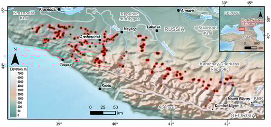
Figure 1. Location of the study area and field plots in the northwestern Caucasus. Field plots are indicated by red circles with black center points, major towns by black circles, and the highest peaks by black triangles. Background elevation is represented by the Cross-blended Hypsometric Tints layer from the Natural Earth dataset [37]. KBR stands for the Kabardino–Balkarian Republic.

The study area has a temperate, humid climate. Average annual temperatures range from 8 to 11 °C, with mean January temperatures of −4 to −5 °C and mean July/August temperatures around 15 °C. Annual precipitation varies considerably, from 500 to 3000 mm. In the mountains, average annual temperature decreases by approximately 0.5 °C per 100 m of elevation, while precipitation increases with altitude, reaching a maximum at 2300–2400 m [38]. Based on elevation, the territory is divided into distinct altitudinal belts [39]: below 200 m—foothill; 200–600 m—low-montane; 600–1400 m—mid-montane; 1400–2000 m—high-montane; 2000–2400 m—subalpine; and above 2400 m—alpine (non-forested). Forest composition varies predictably across these belts:

• In the foothills and low-montane belts, the most widespread forests are oak–hornbeam stands, co-dominated by Carpinus betulus L. and Quercus robur L., Q. petraea (Matt.) Liebl. (sometimes with Q. hartwissiana Stev.). These primarily grow on Greyic Phaeozems Albic or Rendzic Leptosols Eutric soils (on southern slopes). Stands dominated by maple (Acer campestre L., A. platanoides L.), ash (Fraxinus excelsior L.), or black alder (Alnus glutinosa (L.) Gaertn.) are also common.
• The mid-montane and high-montane belts are characterized by forests dominated by oriental beech (Fagus orientalis Lipsky) or co-dominated by beech and fir (Abies nordmanniana (Stev.) Spach), which typically grow on Haplic Cambisols Eutric soils.
• In the high-montane belt, dark coniferous forests of Abies nordmanniana and Picea orientalis (L.) Link become widespread, growing on montane Umbric Albeluvisols Abruptic soils.
• The tree line ends at 1900–2000 m, where birch (Betula pendula Roth, B. litwinowii Doluch.) and maple (Acer trautvetteri Medw., A. pseudoplatanus L.) forests and krummholz communities occur, with rare inclusions of pine (Pinus sylvestris L.), fir, and beech. Pine forests are also frequent in the high-montane and subalpine belts near Mount Elbrus.
• Across all belts, river valleys commonly support stands of grey alder (Alnus incana (L.) Moench) and willow (Salix alba L., S. fragilis L., S. caprea L.) with an admixture of aspen (Populus tremula L.) [40,41].

A long history of anthropogenic impact has led to significant forest reduction in the northwestern Caucasus, exacerbating negative phenomena such as avalanches, mudflows, rockfalls, soil erosion, and habitat loss [33,42,43]. Despite these pressures, the region’s forests remain highly productive [2] and represent unique communities distinguished by a high diversity of endemic and relict flora, performing vital environmental regulation functions [44,45].

2.2. Field Data

Field data were collected in 2014–2024 during systematic surveys of large, homogeneous forest areas (≥100 km²) in the northwestern Caucasus (Figure 1). Specific survey areas and routes were selected based on a visual analysis of open-access satellite imagery and transport accessibility. The routes were organized as transects running perpendicularly across river valleys, extending from the riverbed to the watershed or from the lower to the upper forest line. Along these transects, temporary square sample plots of 100 m² were established at intervals of at least 200 m. Within each plot, a comprehensive forest vegetation relevé was compiled according to standard methodology [46]. This included a complete list of vascular plant species and an estimate of percentage cover for each species within three distinct vegetation layers: the canopy layer (trees > 10 m), the understory layer (shrubs and trees 1–10 m), and the field layer (herbs, dwarf shrubs, and tree/shrub seedlings <1 m). Species cover was visually estimated using the Braun-Blanquet rank scale [15]:

• +: cover <1%;
• 1: cover 1%–5%;
• 2: cover 6%–25%;
• 3: cover 26%–50%;
• 4: cover 50%–75%;
• 5: cover 76%–100%.

From the resulting vegetation database, we selected 558 relevés representing widespread types of deciduous and mixed coniferous–deciduous forests where the upper canopy was composed primarily of broadleaf trees. Dominant tree species included hornbeam (Carpinus betulus), beech (Fagus orientalis), oak (Quercus spp.), maple (Acer spp.), ash (Fraxinus excelsior), aspen (Populus tremula), and birch (Betula pendula), with minor occurrences of black alder (Alnus glutinosa), elm (Ulmus glabra Huds.), and conifers such as fir (Abies nordmanniana), pine (Pinus sylvestris), spruce (Picea orientalis), and yew (Taxus baccata). The selected plots represented a range of naturalness and conservation value. For instance, beech and fir–beech stands were generally well-preserved, while aspen stands were more disturbed and contained numerous non-forest plant species. Consequently, forests with similar canopy composition often differed significantly in their complete floristic composition and syntaxonomic state, reflecting the influence of local ecotope conditions.

2.3. Field Data Classification

The initial field data were classified into forest types using two distinct methodological approaches: floristic and dominant. For each approach, both generalized and detailed classification variants were derived.

2.3.1. Floristic Classification

To perform the floristic classification, the field relevés were compiled into a comprehensive two-way table structured as “plant species (rows) by relevés (columns)”, with cells containing species abundance values. This table was processed and analyzed with the Juice software package (v7.0.99) [47]. The processing involved permuting rows and columns to group together (1) species with similar distribution patterns and ecological requirements (across all layers), and (2) relevés containing similar sets of these grouped species.

The analysis proceeded as follows:

• Species with frequencies between 21% and 80% were grouped based on the similarity of their diagnostic value across vegetation types [48].
• Forest relevés were then clustered based on their compositional similarity, using these groups of diagnostic species.
• Pairwise comparisons between relevé groups were conducted to identify differentiating species. A frequency difference threshold of 40% was applied as a significant indicator of a species’ diagnostic role between two groups [49]. Groups lacking differentiating species were merged, and the procedure was repeated.
• The final groups were considered lower-level syntaxa (associations, subassociations, or variants). To determine their syntaxonomic status, their floristic composition was compared against published data on previously established forest syntaxa in the Caucasian and Euxinian regions [50,51,52,53,54,55,56,57,58,59,60,61,62,63,64,65,66] using a synoptic table. A group was recognized as a new syntaxon if the frequency of species shared with an existing syntaxon differed by more than 40%.

For each confirmed new syntaxon [67,68], diagnostic species were selected from its differentiating species with high frequencies (>20%) based on the Φ (Phi) coefficient, which quantifies species fidelity within a relevé dataset [69]. A threshold of Φ > 30 (p < 0.01) was used to define diagnostic species, an optimal value for forest relevé datasets [70] and one previously applied in the syntaxonomic analysis of Euxinian broadleaf forests [59]. Finally, each new lower syntaxon was assigned to higher-level syntaxa (alliances, orders, classes) based on published prodromus manuals [48,71,72], which provide comparative information on diagnostic species.

2.3.2. Dominant Classification

In its most straightforward implementation, dominant forest classification determines forest type by comparing the proportions of species (or species groups) in the total crown cover (horizontal projection) of the main tree layer. This simple approach is widely used in remote sensing applications, although specific rules—such as species grouping or dominance thresholds—are often case-specific. For this study, we developed a formalized algorithm that enables automatic, similarity-based dominant classification without requiring data-specific assumptions or class-specific threshold adjustments.

The generalized dominant classification was derived through the following steps:

• All tree species were combined into four general groups based on traditional Russian forestry stratification: dark coniferous (spruce, fir, and yew), light coniferous (pine), hard-leaved (beech, elm, hornbeam, oak, maple, and ash), and soft-leaved species (other broadleaf species, including birch, aspen, alder, etc.). Although originally based on wood density, this stratification is ecologically valid because it combines high-level botanical categories (coniferous/broadleaf) with forest successional stages. Light coniferous and soft-leaved groups comprise early-successional species, whereas dark coniferous and hard-leaved groups consist of late-successional species [73,74,75,76].
• For each plot, the proportional contribution of these four groups to the total crown cover was calculated.
• Plots were classified by identifying the minimal Euclidean distance between their species-group fractions and a set of reference fraction patterns representing idealized species combinations (Table 1). These fractions were treated as coordinates in a four-dimensional space, and each plot was assigned to the forest class corresponding to its nearest reference pattern.
  Table 1. Reference species composition patterns and the corresponding generalized forest types for the dominant classification.

  Tree Cover Canopy Fraction for Groups of Species:				Generalized Forest Type
  Dark Coniferous	Light Coniferous	Hard-Leaved Broadleaf	Soft-Leaved Broadleaf
  1.0	0	0	0	Dark coniferous
  0	1.0	0	0	Light coniferous
  0	0	1.0	0	Hard-leaved broadleaf
  0	0	0	1.0	Soft-leaved broadleaf
  0.5	0.5	0	0	Mixed coniferous
  0	0	0.5	0.5	Mixed broadleaf
  0.5	0	0	0.5	Mixed Coniferous–broadleaf
  0	0.5	0.5	0
  0	0.5	0	0.5
  0.5	0	0.5	0
  0.33	0.33	0.33	0
  0.33	0.33	0	0.33
  0.33	0	0.33	0.33
  0	0.33	0.33	0.33
  0.25	0.25	0.25	0.25

Detailed classes were then defined independently within each generalized class to maintain a hierarchical structure. The procedure was as follows:

• The crown-cover fractions of individual tree species were analyzed for each plot. Any plot in which a single species exceeded a crown-cover fraction of 0.5 was assigned to a new class defined by the dominance of that species. Plots lacking a clear dominant species were grouped into a single class of mixed stands.
• For any resulting class containing fewer than 6 plots (representing 1% of the initial dataset), an additional analysis was conducted. If several such small classes were dominated by species from the same generalized group (e.g., dark coniferous, light coniferous, hard-leaved, or soft-leaved) and could be combined to form a group of 6 or more plots, they were merged into a single class defined by the dominance of that species group. Otherwise, plots from these undersized classes were removed from the dataset and excluded from subsequent analyses.

If a generalized class could not be subdivided into two or more detailed classes using this procedure, it remained unchanged and was subsequently used in both the generalized and detailed classification versions.

2.3.3. Comparison of Classifications

To compare the results of the two classification approaches applied to the field data, we employed several standard statistical metrics: the Jaccard Index (JI) [77] for pairwise class comparison and the Modified Adjusted Rand Index (MARI) [78] and Adjusted Mutual Information (AMI) measure [79] for overall concordance assessment.

The Jaccard Index is calculated as the ratio of the number of common elements between two classes to the total number of unique elements across both classes (JI = 1 for identical classes; JI = 0 for completely dissimilar classes). MARI and AMI are widely used in cluster analysis to evaluate the similarity between different clustering results, but they assess concordance differently: MARI is based on pairwise element comparisons, whereas AMI is grounded in information theory. Both metrics are internally normalized and adjusted for chance, with values of 1 indicating perfect concordance and 0 indicating similarity no better than random.

All metrics were computed in the R programming environment (v4.4.2) [80] using the proxy [81] (JI) and aricode [82] (MARI, AMI) packages.

2.4. Geospatial Variables

We utilized a set of well-known, open-access geospatial datasets from the Google Earth Engine (GEE) cloud platform catalog [83] as independent variables for constructing the classification models. Based on their origin and the ecosystem properties they describe, these datasets were grouped into four categories: (1) optical satellite multispectral imagery, (2) a digital elevation model (DEM) and derived characteristics, (3) bioclimatic parameters, and (4) soil properties. All data access and preparatory processing were performed using built-in GEE functionality unless otherwise noted.

2.4.1. Optical Satellite Data

Time series of high-resolution optical multispectral imagery are widely used for geospatial modeling of forest characteristics. Intra-annual changes in spectral reflectance correlate with plant phenology, making metrics derived from these changes valuable for identifying forest species composition.

We utilized data from the Harmonized Landsat–Sentinel-2 (HLS) project [84], which merges Landsat and Sentinel-2 imagery into a unified, global time series with a 30-m spatial resolution and a 2–3-day revisit frequency. The dataset includes surface reflectance (SR) values from ten optical bands (visible, NIR, SWIR) and brightness temperature from the Landsat TIRS1 thermal band. Six SR bands (Blue, Green, Red, NIR, SWIR1, SWIR2) are common to both satellites, while four (three red-edge bands and a “wide” NIR band) are unique to Sentinel-2 [85,86]. In mountainous regions, synchronizing satellite data with specific phenological phases is challenging due to varying dynamics across altitudinal zones. Therefore, we adopted the generalized approach proposed by Pesaresi et al. [87], treating all available pixel-level measurements for each spectral band as points along a continuous intra-annual reflectance curve. These spectral curves were then transformed into geospatial variables using Functional Principal Component Analysis (FPCA), a technique that applies principal component analysis to data represented as measurement series rather than single values.

Because GEE does not provide native FPCA functionality, we performed preliminary statistical aggregation of the satellite time series to reduce computational load. We generated 25 composite images for intra-annual intervals centered from day 1 to day 361 in 15-day increments. Each 29-day wide interval overlapped adjacent intervals by two weeks. For each interval, we created a pixel-level composite by calculating the medoid (the pixel with the minimal Euclidean distance to the band-wise median). Pixels flagged as cloud, cloud shadow, or saturated in the original quality masks were excluded. This aggregation serves as a functional equivalent of smoothing spectral curves using a temporal sliding window. The 15-day step and 29-day interval width were empirically chosen to generate a dense, smooth intra-annual series with maximum spatial coverage while keeping the number of output images manageable.

For all optical bands, we used HLS data from 2020 to 2024 with ≤35% cloud cover (totaling 1459 Landsat and 2328 Sentinel-2 scenes). For the Landsat TIRS1 thermal band, which has lower temporal resolution, we extended the period to 2015–2024, adding 724 scenes to increase data density. The resulting 25 composite images (11 bands each) were exported for local processing. Statistics on valid observations per intra-annual interval are provided in the Supplementary Materials (Table S1).

For each composite image, we calculated normalized ratios in addition to the original spectral bands. These ratios were computed for all unique pairwise combinations of the 10 spectral bands (excluding the TIRS1 thermal band), resulting in 45 ratios per composite. Normalized band ratios [88] are generalized functional analogs of vegetation indices such as NDVI and are calculated as

NR_i+n,i = B_i+n/(B_i + B_i+n),

(1)

where NR_i+n,i is the normalized ratio between bands i + n and i; B_i is the pixel value in band i; B_i+n is the pixel value in band i + n; i ranges from 1 to N-1; n ranges from 1 to N-i; and N is the total number of spectral bands (10 in this case). Band ratios are generally more robust to spatial and temporal variation than raw band values and can provide substantial additional variance for geospatial modeling. However, they tend to be highly correlated, necessitating dimensionality-reduction techniques such as FPCA and rigorous feature selection.

For model training, pixel values were extracted by averaging all pixels within a 50-m radius around each field plot center. The resulting time series were transformed using Functional Principal Component Analysis (FPCA) implemented in the fdapace R package [89]. Gaps in the time series were filled by linear interpolation between adjacent values. FPCA retained 4–8 principal components per spectral band and normalized ratio, capturing at least 95% of the original variance. This process yielded 356 satellite-based variables in total.

2.4.2. DEM and Its Derivatives

We used the 30-m-resolution Copernicus DEM [90] to generate variables characterizing the orographic properties of the study area. In addition to elevation, we derived several morphometric and hydrological indicators.

Morphometric variables were calculated using the MultiscaleDTM R package [91] with a 5 × 5-pixel moving window. These included the following:

• Basic terrain metrics: slope, northness (cosine of aspect), and eastness (sine of aspect).
• Curvature types: mean, minimal, maximal, planar, profile, and twist curvature.
• Complex indices: Topographic Position Index (TPI), Surface Area to Planar Area (SAPA) rugosity, and Vector Ruggedness Measure (VRM).
• Landform classification: flat, slope, pit, channel, pass, ridge, and peak.

Hydrological variables were derived using WhiteboxTools [92] and included distance to stream, cost distance to water, elevation above stream, specific catchment area, Downslope Index, Stream Power Index, Sediment Transport Index, and Topographic Wetness Index.

In total, we generated 28 terrain-related variables: 1 elevation value, 19 morphometric variables, and 8 hydrological indices. Variable values were extracted for each plot using the same method applied to the satellite imagery data.

2.4.3. Bioclimatic Variables

To incorporate the climatic conditions of the study area, we used the standard set of 19 bioclimatic variables from WorldClim version 1 [93]. These variables, provided at a 1 km spatial resolution, represent annual trends, seasonality, and extreme or limiting temperature and precipitation conditions. The set includes the following:

• Temperature-related variables: annual mean temperature (bio1), mean diurnal range (bio2), isothermality (bio3), temperature seasonality (bio4), maximum temperature of the warmest month (bio5), minimum temperature of the coldest month (bio6), temperature annual range (bio7), and mean temperature of the wettest, driest, warmest, and coldest quarters (bio8, bio9, bio10, bio11).
• Precipitation-related variables: annual precipitation (bio12), precipitation of the wettest and driest months (bio13, bio14), precipitation seasonality (bio15), and precipitation of the wettest, driest, warmest, and coldest quarters (bio16, bio17, bio18, bio19).

Values were extracted directly from the coordinates of each plot center.

2.4.4. Soil Features

We used SoilGrids 2.0 [94] to characterize soil properties across the study area. This dataset provides global predictions for 11 soil properties—including silt, sand, clay, and coarse fragment content; pH; bulk density; cation exchange capacity; total nitrogen; and organic carbon content, density, and stock—at a spatial resolution of 250 m. These properties are available for six standard depth intervals (0–5, 5–15, 15–30, 30–60, 60–100, and 100–200 cm), except for organic carbon stock, which is provided only for the 0–30 cm layer. In total, we utilized 61 soil variables. Values for each plot were extracted directly from the plot center coordinates, consistent with the method used for bioclimatic data.

2.4.5. Auxiliary Data

To confirm the absence of destructive forest-cover changes at sample plot locations since the initial surveys, we utilized Google Dynamic World (GDW) data [95]. GDW is a near-real-time, 10-m-resolution dataset based on Sentinel-2 imagery that provides per-pixel probability estimates for nine land-use/land-cover (LULC) classes. For 2024, we created a composite image of the median probability for each LULC class across the study area. We then extracted the mean probability within a 50-m radius around each field plot centre. Any plot for which the “trees” class did not have the highest probability among all classes was excluded from further analysis.

2.4.6. Variable Combinations

The initial composition of variables directly influences a model’s predictive performance and determines both its potential and its limitations. In this study, the geospatial datasets differ in origin, spatial resolution, and the ecological properties they represent. To evaluate the impact of these differences, we tested several distinct initial variable combinations:

• Optical satellite-based variables only;
• High-spatial-resolution variables (satellite- and DEM-based);
• Environmental variables (DEM-based, bioclimatic, and soil);
• All available variables.

All subsequent procedures were performed independently for each of these four variable sets.

2.5. Feature Selection Procedure

We employed a combination of basic and advanced feature selection techniques to optimize the geospatial variable set and to assess the relative informativeness of different data sources prior to model training.

2.5.1. Filtering by Variation and Correlation

We first applied a variance-based filter with a threshold of 0.95 to exclude constant and near-constant variables. Specifically, any variable whose values were identical for more than 95% of the sample plots was removed from further analysis.

Subsequently, we applied correlation-based filtering to the remaining variables. Using the klaR R package [96], we performed hierarchical clustering based on pairwise correlations, treating the correlation magnitude as a distance metric. Variables with a mutual correlation coefficient of 0.95 or higher were assigned to the same cluster. For each variable pair, we computed both Pearson and Spearman coefficients and used the higher absolute value, thereby accounting for both linear and non-linear monotonic relationships and resulting in fewer, more distinct clusters.

For each variable, we then calculated the Average Correlation to the Closest Cluster (ACCC), defined as the highest average correlation between that variable and all variables in another cluster. From each cluster, the variable with the lowest ACCC value was retained as the most informative and least redundant representative of the cluster’s shared information. All other variables in that cluster were excluded.

2.5.2. Filtering by FOCI

In the second stage, we applied the Feature Ordering by Conditional Independence (FOCI) algorithm [97], implemented in the R package of the same name. FOCI is a model-free feature selection method for continuous or binary data that uses the rank-based conditional dependence coefficient (CODEC). CODEC values range from 0 to 1 and can be interpreted as a nonlinear generalization of the partial R² statistic, measuring conditional dependence in a regression context. FOCI utilizes a stepwise forward-selection scheme: at each iteration, it evaluates the CODEC value between the target (response) variable and each candidate independent variable, adding the variable yielding the largest increase in CODEC to the selected set. By default, the selection process stops at the first iteration that yields no improvement in the CODEC value.

For our classification task, FOCI was applied in a one-versus-all manner, converting the multi-class problem into a series of binary classification tasks (one per class). The final variable set comprised all features selected in at least one binary task and was used for subsequent classification model training.

To assess the relative informativeness of each variable in the final set, we used its corresponding CODEC increase rate from the FOCI procedure. To characterize a variable’s overall contribution to class separability, we calculated a weighted average of its CODEC increases across all classes, using the class sample fractions as weights. If a variable was not selected for a particular class, its CODEC increase for that class was set to zero.

2.6. Machine Learning Algorithms

We evaluated two widely used decision tree-based machine learning algorithms—Random Forest (RF) [98] and CatBoost (CB) [99]—alongside two classical classification methods: Linear Discriminant Analysis (LDA) [100], which relies on linear separability between classes, and a k-Nearest Neighbor (kNN) approach [101].

RF constructs an ensemble of decision trees, each trained on random data subsamples, and aggregates their predictions (a process known as “bagging”). We implemented RF using the ranger R package [102] with the splitrule parameter set to “extratrees”, enabling the Extremely Randomized Trees algorithm [103], a faster and more randomized RF variant that can also yield superior performance. In contrast, CB employs an iterative gradient-boosting procedure to construct a single, highly refined decision tree. We implemented CB using the catboost R package [99]. For LDA and kNN, we used the MASS [104] (function lda) and kknn [105] (function kknn) packages, respectively.

All methods include tunable hyperparameters requiring optimization for peak predictive performance. The specific hyperparameters and their values or tuning ranges are provided in the Supplementary Materials (Table S2).

In addition to the four algorithms, we evaluated a simple featureless (variable-free) baseline model that always predicts the most frequent training-set class. This model provides reference performance metrics, enabling quantitative assessment of the value added by the more complex geospatial models.

All procedures for model training, hyperparameter tuning, and performance assessment were implemented using the mlr3 framework in R [106].

2.7. Model Training and Performance Assessment

We employed a 5-fold repeated spatial nested cross-validation (CV) procedure on the initial dataset for model training, hyperparameter tuning, and performance assessment. To create five spatially independent groups of nearly equal size, we used the stratified anti-clustering technique from the anticlust R-package [107]. Unlike traditional clustering, anti-clustering forms groups of equal size by maximizing between-group similarity (i.e., within-group heterogeneity). We used the reciprocal Euclidean distance between field plots (based on XYZ coordinates) as the measure for maximizing within-group diversity. The intersection of the detailed versions of both obtained classifications was used for stratification during anti-clustering, ensuring CV folds with consistent class proportions, albeit with potentially overlapping spatial extents.

The nested CV procedure consisted of the following steps:

• One fold was held out as the test set.
• The remaining folds were used for hyperparameter tuning via an internal CV loop, where each fold served once as a validation set.
• A model was trained on all non-test data using the optimal hyperparameters identified in Step 2.
• The trained model predicted the held-out test fold, and its performance was evaluated.
• Steps 1–4 were repeated until each fold had served as the test set once.
• Performance statistics were aggregated across all five folds.

To address class imbalance, we applied a simple balancing technique during the nested CV procedure: random oversampling (duplication of existing samples) within each training fold, while keeping the test folds unmodified to evaluate performance on the original data distribution. The anti-clustering-based stratification was preserved during this process to ensure equal contributions of all folds to the balanced training sets.

We used the default model-based optimization (MBO) procedure [108] provided by mlr3, running 25 evaluation rounds for automatic hyperparameter tuning. Also known as Bayesian optimization, MBO is a sophisticated “black-box” method that uses a “surrogate model” to efficiently explore the parameter space and typically yields superior results with a limited evaluation budget compared to random or grid search.

Due to the stochastic nature of RF, CB, and MBO, we repeated the entire nested CV procedure 20 times. This allowed us to compute robust statistical summaries—mean, standard deviation, minimum, and maximum—of the performance metrics across all CV folds and repetitions (5 folds × 20 repetitions = 100 evaluations per model configuration).

The Matthews Correlation Coefficient (MCC) was the primary performance metric for both optimization and evaluation. MCC is widely considered an unbiased and informative single measure of classification quality based on the confusion matrix [109]. It generalizes Pearson’s correlation coefficient for two binary variables to multiclass settings. In addition to MCC, we computed two common overall performance metrics:

• Overall accuracy (OAcc)—the proportion of correctly classified cases relative to the total sample size.
• Balanced accuracy (BAcc)—the overall accuracy corrected for class imbalance.

All performance metrics are bounded above by 1, indicating perfect prediction. A value of 0 indicates either a total mismatch (for OAcc and BAcc) or performance equivalent to random guessing (for MCC).

We used the standard paired Wilcoxon test [110] on the MCC values from all CV folds and repetitions to evaluate the statistical significance of differences in mean MCC between models trained with different variable sets and machine learning algorithms. A p-value of 0.01 was used as the significance threshold.

In addition to the overall statistics, we computed standard confusion matrices (CMs) from the cross-validated predictions, along with per-class accuracy metrics:

• Recall—the proportion of correctly classified cases relative to the true class size.
• Precision—the proportion of the correctly classified cases relative to the predicted class size.
• F1-score—the harmonic mean of recall and precision.
• MCC—as described above.

Predictions from all CV folds and repetitions were pooled to compute the CMs. To preserve the initial class-size proportions in the final summaries, the resulting class frequencies were averaged across CV repetitions (i.e., divided by 20).

3. Results

The initial sample of 558 field plots was reduced to 515 during data processing and analysis. The reasons for data omission were as follows:

• Removal of 19 plots due to close placement that resulted in non-unique geospatial variable data.
• Exclusion of 12 plots due to land-cover changes.
• Removal of nine plots representing forest types too small for analysis.
• Exclusion of three plots due to partial gaps in the geospatial variable data.

3.1. Field Data Classification Results

According to the floristic classification approach, the analyzed forests belong to four syntaxa at the order level (Table 2): Carpinetalia betuli (F10—hornbeam forests, approximately 55% of the dataset), Rhododendro pontici–Fagetalia orientalis (F20—beech forests, which may be pure or include a conifer admixture, 38%), Quercetalia pubescenti-petraeae (F30—xerophytic oak forests, 4.5%), and Acero trautvetteri–Betuletalia litwinowii (F40—subalpine mesophytic birch forests, 2.7%).

Table 2. Floristic classification results.

Class ID		Reference Syntaxon Name	Forest Type	Sample Size	Sample Fraction, %
FG	FD
F10		ord. Carpinetalia betuli (within: cl. Carpino-Fagetea)	Hornbeam forests	282	54.8
	F11	ass. Tamo communis–Carpinetum betuli var. typica	Typical mesophytic hornbeam forests	73	14.2
	F12	ass. Aro maculati–Carpinetum betuli	Hygromesophytic hornbeam forests	48	9.3
	F13	ass. Tamo communis–Carpinetum betuli var. Staphylea colchica	Thermophylized mesophytic hornbeam forests	46	8.9
	F14	comm. Abies nordmannianae–Carpinus betulus var. typica	Typical mesophytic hornbeam forests with a small admixture of fir trees	43	8.3
	F15	ass. Tamo communis–Carpinetum betuli var. Festuca drymeja	Xeromesophytic hornbeam forests with a small admixture of sessile oak trees	29	5.6
	F16	comm. Abies nordmannianae–Carpinus betulus var. Juncus effusus	Semi-opened post-cut hygromesophytic hornbeam forests with admixture of quaking aspen and fir trees	18	3.5
	F17	comm. Abies nordmannianae–Carpinus betulus var. Populus tremula	Post-cut mesophytic hornbeam forests with an admixture of quaking aspen and fir trees	16	3.1
	F18	ass. Dryopterido filicis-maris–Carpinetum betuli var. Alnus glutinosa	Post-cut hygromesophytic hornbeam forests with admixture of black alder and fir trees	9	1.7
F20		ord. Rhododendro pontici–Fagetalia orientalis (within: cl. Carpino-Fagetea)	Beech and conifer–beech forests	196	38.1
	F21	ass. Myosotido amoenae–Fagetum orientalis subass. typicum	Typical mesophytic beech forests	90	17.5
	F22	ass. Aro maculati–Fagetum orientalis	Hygromesophytic beech forests	24	4.7
	F23	ass. Lonicero caprifolii–Fagetum orientalis	Xeromesophytic beech forests	22	4.3
	F24	ass. Myosotido amoenae–Fagetum orientalis subass. piceetosum orientalis	Typical mesophytic beech forests with a small admixture of dark-conifer trees (fir, spruce)	21	4.1
	F25	ass. Sambuco nigrae–Fagetum orientalis subass. typicum var. typica	Typical mesophytic mixed fir and beech forests	16	3.1
	F26	ass. Sambuco nigrae–Fagetum orientalis subass. typicum var. Rubus caesius	Semi-opened hygromesophytic mixed fir and beech forests	12	2.3
	F27	ass. Polygonato verticillati–Fagetum orientalis	Post-meadow mesophytic beech forests with a small admixture of pine, aspen, and birch trees	11	2.1
F30		ord. Quercetalia pubescenti-petraeae (within: cl. Quercetea pubescentis)	Xerophytic open oak forests	23	4.5
	F30	ass. Phleo phleoidis–Quercetum petraeae	Xerophytic sessile oak forests	23	4.5
F40		ord. Acero trautvetteri–Betuletalia litwinowii (within: cl. Betulo–Alnetea viridis)	Subalpine open deciduous krummholz and scrub communities	14	2.7
	F40	ass. Rhododendro caucasici–Betuletum litwinowii var. Calamagrostis arundinacea	Subalpine open mesophytic birch forests	14	2.7

Table abbreviations: FG—generalized floristic classification; FD—detailed floristic classification; Sample size—number of field plots per class; Sample fraction—percentage of the total number of field plots per class. Complete syntaxon names are provided in the Supplementary Materials (Table S3).

Alliance names are not designated, as the syntaxonomy of Caucasian forest alliances is still under refinement. The hornbeam forests comprise eight lower-level syntaxa, four of which (F11–F14) account for 75% of this group. The beech forests comprise seven lower-level syntaxa, with typical mesophytic beech forests (F21) alone representing about 50% of this group. Each of the remaining orders, F30 and F40, is represented by a single lower-level syntaxon. In total, the detailed floristic classification includes 17 lower-level syntaxa.

According to the dominant classification approach, the field data were divided into four generalized forest types (Table 3): hard-leaved broadleaf (approximately 74% of the dataset), mixed coniferous–broadleaf (12%), mixed broadleaf (12%), and soft-leaved broadleaf (2.7%) forests.

Table 3. Dominant classification results.

Class ID		Forest Type	Sample Size	Sample Fraction, %
DG	DD
D10		Hard-leaved broadleaf forests:	379	73.6
	D11	with beech dominance	135	26.2
	D12	with hornbeam dominance	103	20
	D13	with mixed composition	83	16.1
	D14	with oak dominance	52	10.1
	D15	with ash dominance	6	1.2
D20		Mixed coniferous–broadleaf forests:	62	12
	D21	with mixed composition	23	4.5
	D22	with beech dominance	22	4.3
	D23	with fir dominance	9	1.7
	D24	with hornbeam dominance	8	1.6
D30		Mixed broadleaf forests:	60	11.7
	D31	with hard-leaved dominance	32	6.2
	D32	with soft-leaved dominance	28	5.4
D40		Soft-leaved broadleaf forests:	14	2.7
	D40	with birch dominance	14	2.7

Table abbreviations: DG—generalized dominant classification; DD—detailed dominant classification; Sample size—number of field plots per class; Sample fraction—percentage of the total number of field plots per class.

The hard-leaved broadleaf type consisted of five detailed classes, including forests dominated by beech (36% of this generalized type), hornbeam (27%), oak (14%), and ash (1.5%) species, along with mixed stands (22%) without a single dominant species. The mixed coniferous–broadleaf type included four detailed classes—mixed stands (37%) and forests dominated by beech (35%), fir (15%), and hornbeam (13%) species. The mixed broadleaf type was divided into two detailed classes of nearly equal size, representing hard-leaved- and soft-leaved-dominated stands. Each class was formed by combining several small groups dominated by different species that were individually too small to be considered separate classes. Finally, the soft-leaved broadleaf type, represented by birch-dominated stands, had no detailed subdivisions. In total, the detailed dominant classification consisted of 12 forest types.

The pairwise comparison of class assignments between the two classifications, based on the Jaccard Index (JI), is shown in Figure 2. Only the floristic subalpine open mesophytic birch forests (F40) and the dominant soft-leaved broadleaf forests with birch dominance (D40) had identical compositions. In contrast, most generalized and detailed classes had JI values close to zero. The hard-leaved broadleaf forests (D10) of the dominant classification showed moderate overlap with the floristic hornbeam (F10) and beech (F20) forests, with JI values of 0.45 and 0.36, respectively. Among the detailed classes, only three pairs demonstrated moderate similarity:

Figure 2. Pairwise Jaccard index matrices comparing the floristic and dominant classifications: (a) generalized classes; (b) detailed classes. Class designations follow Table 2 and Table 3.

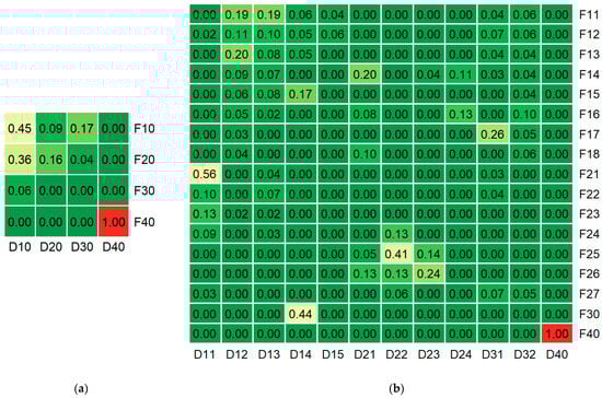
• Typical mesophytic beech forests (F21) and hard-leaved broadleaf forests with beech dominance (D11) (JI = 0.56);
• Typical mesophytic mixed fir and beech forests (F25) and mixed coniferous–broadleaf forests with beech dominance (D22) (JI = 0.41);
• Xerophytic sessile oak forests (F30) and hard-leaved broadleaf forests with oak dominance (D14) (JI = 0.44).

For the generalized classifications, we obtained an MARI of 0.03 and an AMI of 0.16, and for the detailed variants, the respective values were 0.27 and 0.35. These low index values indicate low overall concordance between the two classification systems for both variants and complement the predominantly low pairwise JI values.

3.2. Feature Selection Results

The final number of variables selected for training the classification models ranged from 9 to 67, depending on the classification type and the composition of the original dataset (Table 4). On average, detailed classification types required 2–3 times more variables than generalized types.

Table 4. Aggregated results of the feature selection procedure using the FOCI algorithm.

Classification Type	Initial Variable Set	N	CODEC, %	CODEC/N, %	CODEC by Variable Type, %
					Sat	DEM	WCB	Soil
Floristic Generalized	All	9	86.4	9.6	2.3	2.1	77.5	4.5
	Env	10	89.1	8.9	–	0.0	82.8	6.3
	HiRes	13	86.0	6.6	19.8	66.2	–	–
	Sat	19	86.9	4.6	86.9	–	–	–
Floristic Detailed	Env	28	66.7	2.4	–	2.2	42.2	22.4
	All	48	71.2	1.5	15.1	2.2	29.3	24.6
	HiRes	67	71.5	1.1	53.0	18.5	–	–
	Sat	65	67.5	1.0	67.5	–	–	–
Dominant Generalized	Env	11	60.3	5.5	–	0.7	37.6	22.1
	All	15	65.2	4.3	11.1	2.2	38.4	13.5
	HiRes	16	60.5	3.8	30.7	29.8	–	–
	Sat	21	67.4	3.2	67.4	–	–	–
Dominant Detailed	Env	28	53.8	1.9	–	1.6	31.0	21.2
	HiRes	34	55.7	1.6	34.7	21.0	–	–
	All	37	59.7	1.6	16.1	2.8	32.1	8.8
	Sat	37	56.8	1.5	56.8	–	–	–

Table abbreviations: N—the number of selected features; CODEC—averaged cumulative value of the conditional dependence coefficient; Sat—optical satellite-based variables; DEM—DEM-based variables; WCB—WorldClim bioclimatic variables; Soil—SoilGrids variables; All—set of all available variables; Env—set of environmental variables; HiRes—set of high-spatial-resolution variables.

Average cumulative CODEC values ranged from 54% to 89%, with systematically higher rates for the floristic classification versus the dominant classification, and for generalized variants versus detailed ones. Differences among initial variable sets within the same classification type were relatively small (3 to 7 percentage points (p.p.)).

The environmental variable set was the most effective initial data combination in terms of average CODEC per selected variable for the detailed floristic classification and for both variants of the dominant classification. For the generalized floristic classification, the environmental set also had the highest CODEC but was less effective on a per-variable basis than the full-variable set. The initial set of high-spatial-resolution variables had the highest total CODEC value for the detailed floristic classification, the optical satellite-based set for the generalized dominant classification, and the full-variable set for the detailed dominant classification.

Bioclimatic variables had the highest averaged cumulative CODEC values (29%–83%) within both the environmental and full-variable sets for all classification types, followed by SoilGrids variables (5%–25%) in all cases except the detailed dominant classification with the full-variable set, where satellite-based variables were more effective. Generally, DEM-based variables had the lowest impact on CODEC values (0%–3%) in the environmental and full-variable sets but performed roughly on par with the satellite-based variables in the high-resolution set. While satellite-based variables had a relatively low impact within the full-variable set (2%–16%), they provided highly competitive cumulative CODEC values when used alone, albeit at the cost of requiring a larger number of selected variables.

The final variable sets selected for different classification types generally had distinct compositions, with only 2%–40% of variables in common (Figure 3). This pattern persisted when considering only the five most effective variables (by CODEC increase) from each set. The detailed variants of the floristic and dominant classifications shared the largest fraction of variables (40%) when the environmental initial set was used; when the full-variable initial set was used, the top-five overlap was 43% (3 of 7). The intersections between generalized and detailed variants of the same classification type (floristic or dominant) exhibited equal or lower overlap rates than inter-type comparisons.

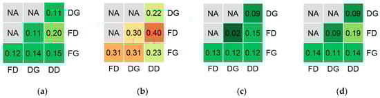
Figure 3. Pairwise fractions of shared variables selected for different classification types, depending on the initial variable set: (a,e) all available variables; (b,f) environmental variables; (c,g) high-spatial-resolution variables; (d,h) optical satellite-based variables. The upper row (a–d) shows results for the entire selected variable set; the lower row (e–h) shows results for the top five most effective variables in each set. Classification types: FG—floristic generalized; FD—floristic detailed; DG—dominant generalized; DD—dominant detailed.

Among the top features selected from the full-variable initial set, bioclimatic variables demonstrated the highest impact and frequency (Table 5). WorldClim temperature seasonality (standard deviation of monthly temperatures) was the only variable ranked among the top five across all classification types and had the highest average CODEC value for both the detailed floristic and the generalized dominant classifications. For the generalized floristic classification, mean temperature of the wettest quarter, minimum temperature of the coldest month, and precipitation of the coldest quarter collectively accounted for over 75 of the total 86.4 p.p. of the cumulative CODEC. Precipitation of the warmest quarter was the most effective variable for the detailed dominant classification.

Table 5. The five most effective variables selected from the full-variable initial set for each classification type.

Variable Type	Variable Description	CODEC, %
		FG	FD	DG	DD
WCB	Temperature seasonality (standard deviation)	2.2	12.0	37.6	4.5
Soil	Cation exchange capacity in the 0–5 cm layer	2.3	2.3	2.3	3.1
WCB	Precipitation of the warmest quarter	0.0	5.3	0.9	17.5
WCB	Precipitation of the coldest quarter	7.6	7.2	0.0	6.5
WCB	Mean temperature of the wettest quarter	38.0	1.3	0.0	0.0
WCB	Mean of monthly temperature ranges (diurnal range)	0.0	1.9	0.0	3.4
Soil	Organic carbon density in the 0–5 cm layer	0.0	0.6	2.6	0.0
WCB	Minimal temperature of the coldest month	29.6	0.0	0.0	0.0
Soil	Total nitrogen content in the 15–30 cm layer	0.0	0.0	7.6	0.0
Sat	FPC7 of the NR between RE2 and RE3 spectral bands	0.0	0.0	7.4	0.0
Soil	Bulk density of the fine earth fraction in the 15–30 cm layer	0.0	6.1	0.0	0.0
Soil	Total nitrogen content in the 0–5 cm layer	0.0	5.8	0.0	0.0
Sat	FPC4 of the Green spectral band	0.0	0.0	0.0	4.0

Table abbreviations: CODEC—averaged value of the conditional dependence coefficient by classification type (the top 5 values for each are in bold): FG—floristic generalized; FD—floristic detailed; DG—dominant generalized; DD—dominant detailed; WCB—WorldClim bioclimatic variables; Soil—SoilGrids variables; Sat—satellite-based variables; FPCn—n-th functional principal component; NR—normalized ratio; RE2, RE3—2nd and 3rd red-edge spectral bands.

SoilGrids variables—including total nitrogen content (0–5 and 15–30 cm layers), cation exchange capacity (0–5 cm), soil bulk density (15–30 cm), and organic carbon density (0–5 cm)—appeared in the top-five lists for all cases except the detailed dominant classification, but with significantly lower CODEC values. Optical satellite-based variables had minor representation in the top rankings only for the dominant classification variants. No DEM-based variables were among the most effective features for any classification type.

The full list of selected features and their averaged CODEC values for each classification type and initial variable set is provided in the Supplementary Materials (Tables S4–S7).

3.3. Models’ Overall Performance

According to the performance evaluation results (Table 6), the best predictive models for the generalized floristic classification achieved mean MCC values of 80%–84%, with a corresponding overall accuracy (OAcc) of 89%–91% and a balanced accuracy (BAcc) of 83%–91%, depending on the variable set used. The analogous models for the generalized dominant classification yielded noticeably lower metrics, with MCC values of 54%–60%, OAcc of 80%–83% and BAcc of 70%–76%. Performance further decreased for the detailed classification variants: the floristic models had MCC values of 44%–53%, OAcc of 48%–56%, and BAcc of 51%–58%, while the dominant models had MCC values of 41%–44%, OAcc of 49%–52%, and BAcc of 43%–47%.

Table 6. Aggregated performance statistics for the optimal classification models.

Classification Type	Variable Set	Best MLA	MCC, %				Overall Accuracy, %				Balanced Accuracy, %
			Min	Mean	Max	SD	Min	Mean	Max	SD	Min	Mean	Max	SD
Floristic Generalized	All	RF	74.4	84.4	96.6	7.7	83.5	90.9	98.1	4.8	81.1	91.4	99.1	5.7
	HiRes	RF	68.6	83.8	94.7	9.3	81.6	90.6	97.1	5.7	63.7	87.4	97.7	10.1
	Env	CB	68.8	82.7	96.6	8.7	80.6	90.0	98.1	5.3	74.8	89.0	99.1	6.8
	Sat	RF	58.9	80.4	98.2	11.8	77.7	88.9	99.0	6.7	49.1	83.0	93.8	13.0
	none	Ref	0.0	0.0	0.0	0.0	53.4	54.8	55.3	0.9	25.0	25.0	25.0	0.0
Floristic Detailed	All	CB	35.8	52.8	71.5	9.5	40.8	56.2	73.8	9.1	46.1	58.0	72.9	6.5
	HiRes	CB	35.3	50.4	62.7	7.6	39.8	54.5	66.0	7.3	40.5	51.4	60.8	4.9
	Sat	CB	36.9	48.9	68.0	8.9	42.7	53.3	70.9	8.2	41.2	50.3	64.0	5.6
	Env	CB	33.6	44.3	57.5	6.0	36.9	47.8	60.2	6.1	38.3	50.6	59.8	4.6
	none	Ref	0.0	0.0	0.0	0.0	17.5	17.5	17.5	0.0	5.9	5.9	5.9	0.0
Dominant Generalized	All	RF	53.2	59.9	66.6	2.7	78.6	83.4	86.4	1.9	63.1	72.6	78.7	4.0
	Env	RF	51.4	58.3	70.9	4.4	73.8	81.3	86.4	2.5	66.7	76.4	85.8	5.6
	HiRes	RF	44.1	55.3	62.8	3.5	76.7	80.7	84.5	1.6	55.1	73.2	82.0	6.0
	Sat	RF	42.5	53.6	71.8	6.3	71.8	80.4	88.3	3.9	59.7	69.8	78.1	4.4
	none	Ref	0.0	0.0	0.0	0.0	72.8	73.6	74.8	1.1	25.0	25.0	25.0	0.0
Dominant Detailed	HiRes	RF	32.1	44.0	50.5	4.7	40.8	52.1	58.3	4.4	40.1	46.4	60.2	6.3
	All	RF	33.3	43.9	52.3	4.6	41.7	51.9	59.2	4.3	35.8	47.2	61.4	6.2
	Sat	RF	31.8	42.7	53.1	4.8	41.7	51.1	60.2	4.3	33.6	43.3	55.5	3.3
	Env	CB	22.9	40.7	54.0	8.3	33.0	49.4	61.2	7.3	35.4	45.7	60.8	6.5
	none	Ref	0.0	0.0	0.0	0.0	26.2	26.2	26.2	0.0	8.3	8.3	8.3	0.0

Table abbreviations: Variable set—origin of the optimized variable subset used for model training (sets in bolds have a significantly higher mean MCC value compared to regular sets, according to the Wilcoxon test); All—all available variables; HiRes—high spatial resolution variables; Env—environmental variables; Sat—optical satellite-based variables; Best MLA—machine learning algorithm that yielded the highest mean MCC for a particular variable set (algorithms in bold indicate a statistically significant difference in mean MCC compared to all other algorithms); RF—Random Forest; CB—CatBoost; Ref—featureless reference model; min, mean, max, SD—minimum, mean, maximum, and standard deviation values of performance metrics calculated across all cross-validation folds and repetitions.

According to the Wilcoxon test, models using variables from the full set of available data significantly outperformed those using other variable sets in most cases, as measured by the mean MCC. The exceptions were high-resolution variables for the generalized floristic and detailed dominant classifications, and the environmental variables for the generalized dominant classification, where models from two different variable sets performed on par.

Random Forest (RF) and CatBoost (CB) exhibited significantly better average performance than LDA and kNN across all analyzed cases. RF was the top-performing algorithm for both generalized classifications, while CB performed best for the detailed floristic classification. For the detailed dominant classification, RF and CB performed on par. Aggregated performance metrics for all models are presented in the Supplementary Materials (Table S8).

The best geospatial classification models outperformed the respective featureless reference models for all classification types. Spatial modeling increased the mean OAcc by 10 to 39 p.p., with the smallest gain for the generalized dominant classification and the largest for the detailed floristic classification. The mean BAcc increased even more substantially, by 39 to 66 p.p.

3.4. Models’ Classification Accuracy

The cross-validated predictions of the most effective models (based on the filtered variable set) are shown in the confusion matrices in Figure 4, with corresponding per-class accuracy statistics in Table 7 and Table 8.

Figure 4. Normalized confusion matrices from the cross-validated predictions of the optimal models for (a) generalized and (b) detailed floristic classifications; (c) generalized and (d) detailed dominant classifications. Rows represent observed classes, and columns represent predicted classes. Cell values represent the percentage of observations for a given class (rows) that were predicted as each class (columns); matrices are normalized by row sums. Class abbreviations are the same as in Table 2 and Table 3.

Table 7. Per-class accuracy statistics for the optimal floristic classification models.

Class ID		Forest Type	Accuracy, %
FG	FD		Recall	Precision	F1	MCC
F10		Hornbeam forests	91.0	92.4	91.7	81.8
	F11	Typical mesophytic hornbeam forests	52.1	58.3	55.1	48.2
	F12	Hygromesophytic hornbeam forests	79.8	75.7	77.7	75.4
	F13	Thermophylized mesophytic hornbeam forests	55.3	46.4	50.5	45.4
	F14	Typical mesophytic hornbeam forests with a small admixture of fir trees	56.6	52.4	54.4	50.2
	F15	Xeromesophytic hornbeam forests with a small admixture of sessile oak trees	12.2	18.7	14.8	11.1
	F16	Semi-opened post-cut hygromesophytic hornbeam forests with an admixture of quaking aspen and fir trees	74.7	76.4	75.6	74.7
	F17	Post-cut mesophytic hornbeam forests with an admixture of quaking aspen and fir trees	73.1	59.7	65.7	64.9
	F18	Post-cut hygromesophytic hornbeam forests with an admixture of black alder and fir trees	71.7	64.2	67.7	67.2
F20		Beech and conifer–beech forests	91.0	91.0	91.0	85.4
	F21	Typical mesophytic beech forests	58.3	71.2	64.1	57.8
	F22	Hygromesophytic beech forests	36.5	27.5	31.3	27.8
	F23	Xeromesophytic beech forests	6.4	7.2	6.7	2.8
	F24	Typical mesophytic beech forests with a small admixture of dark-conifer trees (fir, spruce)	51.2	56.1	53.6	51.7
	F25	Typical mesophytic mixed fir and beech forests	71.9	62.3	66.8	65.8
	F26	Semi-opened hygromesophytic mixed fir and beech forests	48.3	49.6	49.0	47.8
	F27	Post-meadow mesophytic beech forests with a small admixture of pine, aspen, and birch trees	76.4	43.4	55.4	56.4
F30		Xerophytic open oak forests	82.2	74.0	77.9	76.9
	F30	Xerophytic sessile oak forests	69.1	68.7	68.9	67.5
F40		Subalpine open deciduous krummholz and scrub communities	100.0	89.7	94.6	94.6
	F40	Subalpine open mesophytic birch forests	92.9	88.4	90.6	90.4

Table abbreviations: FG—class IDs for the generalized classification variant; FD—class IDs for the detailed classification variant.

Table 8. Per-class accuracy for the optimal dominant classification models.

Class ID		Forest Type	Accuracy, %
DG	DD		Recall	Precision	F1	MCC
D10		Hard-leaved broadleaf forests	92.5	87.9	90.1	60.1
	D11	with beech dominance	83.4	75.2	79.1	71.3
	D12	with hornbeam dominance	45.8	48.0	46.9	34.0
	D13	with mixed composition	14.5	29.4	19.4	10.6
	D14	with oak dominance	74.0	50.3	59.9	55.8
	D15	with ash dominance	20.0	16.4	18.1	17.1
D20		Mixed coniferous–broadleaf forests	82.1	77.2	79.6	76.7
	D21	with mixed composition	59.4	36.9	45.5	43.7
	D22	with beech dominance	61.4	41.7	49.7	48.0
	D23	with fir dominance	20.0	26.7	22.9	21.9
	D24	with hornbeam dominance	48.8	31.6	38.3	38.1
D30		Mixed broadleaf forests	24.8	42.4	31.3	25.9
	D31	with hard-leaved dominance	22.8	26.8	24.7	20.2
	D32	with soft-leaved dominance	8.8	19.6	12.1	9.9
D40		Soft-leaved broadleaf forests	92.9	87.3	90.0	89.7
	D40	with birch dominance	93.6	92.9	93.2	93.1

Table abbreviations: FG—class IDs for the generalized classification variant; FD—class IDs for the detailed classification variant.

At the per-class level, the optimal model for the generalized floristic classification demonstrated consistently high accuracy. Oak forests (F30) had the lowest accuracy, with an MCC of 77% (F1-score = 78%) due to confusion with hornbeam forests (F10). Subalpine open forests (F40) had the highest individual accuracy, with both the MCC and F1-score at 95%. Hornbeam (F10) and beech (F20) forests showed minor mutual confusion, resulting in MCC values of 82% (F1-score = 92%) and 85% (F1-score = 91%), respectively.

Among the detailed floristic types, only hygromesophytic hornbeam forests (F12) and semi-opened post-cut hygromesophytic hornbeam forests with an admixture of quaking aspen and fir trees (F16)—in addition to subalpine birch forests (F40)—achieved relatively high accuracy, with MCC values of about 75% and F1-scores of 76%–78%. In contrast, xeromesophytic beech forests (F23) were confused with various hornbeam (F12, F13) and beech (F21, F22, F24) forest types and demonstrated the lowest separability, with an MCC of only 3% (F1-score = 7%). Xeromesophytic hornbeam forests with a small admixture of sessile oak trees (F15) were also largely misclassified as other hornbeam types (F11, F13, F14) and oak forests (F30), resulting in an MCC of 11% (F1-score = 15%). Hygromesophytic beech forests (F22) demonstrated the third-worst accuracy, with an MCC of 28% (F1-score = 31%), mainly due to confusion with typical mesophytic beech forests (F21) and hygromesophytic hornbeam forests (F12). The remaining classes showed mediocre-to-moderate accuracy, with MCC values of 45%–67% and F1-scores of 49%–69%, primarily due to confusion within their respective generalized classes. Notably, typical mesophytic mixed fir and beech forests (F26) and semi-opened hygromesophytic mixed fir and beech forests (F25) were almost exclusively confused with each other, suggesting that merging these classes could improve classification accuracy.

Overall, the geospatial models for the floristic classification provided reliable results at the order level and moderate separability for most lower-level syntaxa (alliances and associations), except for xeromesophytic hornbeam and beech forests, which demonstrated extremely low predictive accuracy.

For the generalized dominant classification, the per-class accuracy results were significantly lower than those for the floristic classification. Soft-leaved broadleaf forests (D40, identical to floristic F40) exhibited the best performance, with an MCC and F1-score of 90%. In contrast, mixed broadleaf forests (D30) achieved an MCC of only 26% (F1-score = 31%) due to high confusion with hard-leaved broadleaf forests (D10). The latter, being the largest class in terms of sample size, had a high F1-score of 90%, but only a 60% MCC because of substantial confusion with the D20 and D30 classes. Mixed coniferous–broadleaf forests (D20) exhibited more balanced accuracy metrics, with moderate confusion (MCC of 77%, F1-score = 80%).

For the detailed dominant classification and excluding soft-leaved birch-dominated forests (D40, identical to F40), only the most frequent detailed class—hard-leaved broadleaf forests with beech dominance (D11)—achieved an MCC above 70%, with an F1-score of 79%. Oak-dominated forests (D14) were heavily confused with other hard-leaved broadleaf classes, resulting in moderate accuracy (MCC of 56%, F1-score of 60%). The remaining classes demonstrated low-to-mediocre separability, with MCC values of 10%–48% and F1-scores of 12%–50%. Most had a broad set of confused classes, including those belonging to different generalized types. Both sub-classes of mixed broadleaf forests (D31, D32) and mixed hard-leaved broadleaf forests (D13) showed notably low accuracy (MCC values of 10%–20%, F1-scores of 12%–25%). Thus, reliably differentiating individual broadleaf dominant species and their mixtures appears extremely challenging with the available geospatial data. Classes dominated by ash (D15) and fir (D23) also exhibited low separability (MCC values of 17%–22%, F1-scores of 18%–23%), likely due to their initially small sample sizes (six and nine plots)

Overall, the geospatial models for the dominant classification demonstrated moderate performance at the generalized level and low-to-mediocre accuracy for most detailed classes. Broadleaf forests with highly mixed species compositions are naturally the most difficult target for model-based identification of dominants.

4. Discussion

4.1. Study Limitations

Aside from the specific area and object of our study, the generalizability of the results is naturally constrained by the properties of the initial data and the methodology used. The main sources of these limitations are as follows:

• Potential sampling bias. The mountainous study area precludes spatially regular or randomized sampling designs. Although the reference field dataset is sufficiently large and well distributed, it was not originally collected for geospatial modeling. Consequently, its establishment relied more on expert judgment than on statistically rigorous design. This may result in incomplete representation of certain environmental conditions, potentially reducing the reliability of model predictions for areas distant from the sampled plots.
• Relatively small field plot size. Establishing large plots in mountainous terrain is difficult. Although a 100 m² plot size is acceptable for forest vegetation relevés and sufficient for floristic analyses [111], it is small relative to the pixel sizes of most open-access geospatial datasets, including those used here. Scale mismatches combined with georeferencing errors may cause discrepancies between plot characteristics and the values of corresponding pixels, which may negatively affect both feature selection and model performance.
• Predictive nature of the environmental variables. WorldClim, Copernicus DEM, and SoilGrids are outputs of geospatial modeling and have inherent uncertainties. They therefore cannot be fully equated with direct measurements. Consequently, the results of feature selection and variable informativeness should be viewed as tools for model optimization under the given data conditions rather than as evidence for ecological cause-and-effect relationships.
• Implementation-specific aspects of forest-type classification. Although the general principles of the floristic and dominant classifications are known, the exact rules and algorithms are not fully standardized. Consequently, practical implementations depend heavily on the researcher’s experience, and results may differ even when the same dataset is processed by different individuals.
• Feature selection performed outside the nested cross-validation loop. To reduce computational time, feature selection was performed on the full dataset before spatial cross-validation. This may inflate the resulting accuracy metrics, as the test data cannot be considered completely unseen. For fully unbiased accuracy estimates, feature selection must be incorporated into the nested cross-validation procedure.

In the context of this study, these limitations have minimal impact on the main findings, as the comparison of classification approaches was performed on the same data using a unified methodology. However, they must be considered when comparing or extrapolating our specific estimates (e.g., accuracy scores, CODEC values, optimized variable sets) to other study areas and datasets.

4.2. Comparison of the Classification Results

As mentioned in the Introduction, different classification approaches rarely produce classes with similar compositions, even when applied to the same initial dataset [18], and our results are fully consistent with this pattern. Only subalpine birch forests are consistently distinguished from the main massif of broadleaf and coniferous–broadleaf forests in both the floristic and dominant classifications. Their separation is expected, given their contrasting species composition and specific growing conditions within the mountain ecosystem. For all other forests with more complex species composition, the similarity between classes derived from the two approaches remains minimal because many species occupy overlapping ecological niches. This highlights the critical importance of the initial choice of classification approach when preparing training data for geospatial modeling, as such substantial differences severely limit the possibility of analytically converting one classification into another without direct reference to field data.

These differences in class composition inevitably lead to equally pronounced differences in the optimal variable sets selected for model construction. This applies not only to classifications based on different approaches but also to classifications at different hierarchical levels within the same approach. These findings highlight the need for a task-specific feature selection procedure as an essential step for balancing model complexity and performance.

4.3. Feature Selection

Despite their coarse spatial resolution (especially compared to the field-plot size), WorldClim and SoilGrids variables were unexpectedly more effective than the satellite- and DEM-derived variables. In many recent regional-scale forest–species mapping studies, remote sensing imagery and its derivatives are used as the primary predictors due to their higher temporal and spatial resolution [21,23,112,113,114], while environmental variables (usually DEM-based) serve as optional supporting predictors for further model refinement [19,20,22,87,115]. Although coarse datasets such as WorldClim and SoilGrids are rarely combined with high-resolution satellite imagery, they can significantly improve tree-species mapping accuracy in certain cases [116].

The influence of climatic and soil variables on forest-type distribution is usually most evident in large-scale studies spanning a wide range of habitat conditions across several biomes [18,117] and may be weak in small regions. However, in mountainous regions, altitudinal zonation compresses various natural conditions into a relatively compact area, preserving the relevance of these variables even at a local scale.

The relatively small positive effect of combining all available variables on the total explained variation (cumulative CODEC values) suggests that different variable groups may contain similar useful information. This is unsurprising, given that WorldClim and SoilGrids are themselves products of geospatial modeling and thus already integrate variance from their original predictors, including topographic, climatic, and vegetation data, often derived from satellite imagery. Within this context, bioclimatic and soil variables often outperform generic DEM-based and optical satellite-based variables during feature selection, as they provide more complete and effective proxies (in terms of useful variance per variable) for the main drivers of forest-ecosystem distribution. This is consistent with the optimization results from the high-resolution initial variable set, which excluded WorldClim and SoilGrids. In this case, DEM elevation, representing the most direct driver of habitat conditions in mountainous regions, emerged as the most informative variable for all classification variants (see Table S5 in the Supplementary Materials), while the total explained variance remained similar. Although optical satellite-based variables can explain a comparable amount of variance, they nearly double the size of the optimal variable set even after data-compression techniques such as FPCA, reducing their efficiency relative to environmental variables.

Variable importance is also affected by data quality. Modern global DEMs (including the Copernicus DEM used here) represent the Earth’s surface, not the actual terrain. Because the forest canopy almost completely masks the microtopography, many morphological and hydrological indices derived from these DEMs perform poorly when related to small ground plots, as clearly observed in our study. SoilGrids data, derived from global modeling of soil characteristics based on spatially inconsistent training data, particularly for the Russian Federation, also have limited reliability at regional and local scales. Their primary predictors largely overlap with the climate and terrain variables used in our study. Nevertheless, SoilGrids still contributed a small amount of additional useful information when combined with bioclimatic variables. For instance, the cation exchange capacity (in the 0–5 cm layer), an indicator of soil fertility, was included in the optimized variable sets for all classification types. Other soil variables, such as bulk density and carbon and nitrogen content, were strongly type-specific, consistent with previous studies on soil variables in tree-species distribution modeling [116,118].

Overall, the most robust strategy is to use the broadest possible set of all available geospatial variables and then optimize this set for the specific reference data. However, different initial combinations of task-relevant variables can yield similar cumulative CODEC values and final model accuracies, allowing flexibility based on the research. For example, high-resolution satellite data could be used for fine-scale digital mapping of current forest types, whereas less detailed but more interpretable environmental variables may be more suitable for predicting changes in their spatial distribution under shifting environmental conditions.

4.4. Model Performance Comparison

Floristic classification models outperformed dominant classification models at both the generalized and detailed levels. Therefore, our case study provides a convincing example of a situation in which the more complex floristic approach yields more informative and reliable results, not only from an ecological perspective but also for geospatial modeling. Moreover, such situations are not necessarily limited to mountainous forests, as comparable findings, though based on more limited data and a simplified methodology, have been reported for mixed coniferous–deciduous stands located in the southwest of the Moscow region [119]. Extending comparative analyses of this kind to additional regions may help clarify the applicability domains of dominant and floristic classification approaches in the context of geospatial modeling and mapping of forest types and attributes.

Machine learning methods based on decision trees, particularly variants of Random Forests, are now the de facto standard for complex classification tasks in geospatial modeling [120]. Therefore, the superior performance of Extremely Randomized Trees and CatBoost in our benchmark was largely expected.

4.5. Separability of Forest Types

Generalized forest types, especially under the floristic classification, demonstrated sufficient separability in the resulting geospatial models. However, reliable discrimination among detailed classes remained considerably more challenging for both classification approaches. Reported overall accuracies for the forest-type classification models typically range between 50 and 90 p.p. (with even broader ranges for individual classes) and depend heavily on the number and level of detail of the classes considered [121,122,123]. Higher levels of generalization produce higher predictive accuracy, regardless of the chosen classification approach, and our results confirmed this trend.

The moderate-to-low separability of detailed classes may reflect the limited reliability of the available data (small field plots combined with the coarse spatial resolution of geospatial variables) and the absence of additional variables representing unaccounted but influential factors in forest ecosystem functioning and development. These limitations are difficult to overcome. Most publicly available geospatial data suitable for modeling rely on the same or similar sources used in this work. Obtaining higher-quality data for forest mapping would require broader adoption of more sophisticated measurement methods, such as laser scanning, to derive detailed terrain and tree canopy models. Likewise, incorporating additional environmental factors would require extensive expert analysis of alternative sources of information (if available), such as historical maps and documents, to reconstruct landscape dynamics and the degree of human influence. Both approaches require substantial time, labor, and financial resources, with limited economic incentives, particularly in remote mountainous areas, where forests are generally valued more for conservation value than for industrial use.

5. Conclusions

In this study, we compared a complex, expertise-based floristic classification with a simpler, formalized approach based on species dominance. The goal was to assess their ability to produce clearly distinguishable forest types suitable for geospatial modeling-based forest mapping under the same data conditions. We derived floristic and dominant classification variants for the same dataset of field plots, representing mixed and broadleaf forests of the northwestern Caucasus. We then compared the resulting classes and evaluated the performance of geospatial models trained on these datasets and spatial variables from different sources. The comparison yielded the following findings:

• The forest types identified by the two approaches had very little in common at both generalized and detailed levels. This is a natural outcome for complex, multi-dominant tree stands.
• The optimal variable sets for geospatial modeling differed substantially between the two classification approaches and between their generalized and detailed variants. Task-specific feature selection is therefore an essential step in model development.
• Bioclimatic and soil variables were unexpectedly more informative than DEM-based and optical satellite-based variables, despite their coarser spatial resolution. This is likely due to the mountainous nature of the study region.
• Floristic-based geospatial models clearly outperformed dominant-based models in terms of forest-type separability and predictive accuracy. Therefore, the floristic classification approach may be preferable for forests with complex species composition, both ecologically and in terms of the reliability of geospatial modeling and derived mapping results. However, accuracy still depends heavily on the desired level of detail. Although generalized forest types demonstrated sufficient separability, detailed classes achieved only moderate-to-low separability.

These findings may support future studies on geospatial modeling and mapping of forest types in the Caucasus or similar mountainous regions, characterized by relief and/or complex tree-stand composition. Future work will focus on expanding the reference dataset with vegetation relevés from coniferous and mixed broadleaf–coniferous forests in the region. These data will be used to train a more comprehensive and robust geospatial model for producing a floristic-based forest-type map of the northwestern Caucasus.

References

- Myers, N.; Mittermeier, R.A.; Mittermeier, C.G.; Da Fonseca, G.A.B.; Kent, J. Biodiversity hotspots for conservation priorities. Nature 2000, 403, 853–858. [Google Scholar] [CrossRef]
- Shevchenko, N.E.; Kuznetsova, A.I.; Tebenkova, D.N.; Smirnov, V.E.; Geraskina, A.P.; Gornov, A.V.; Grabenko, E.A.; Tikhonova, E.V.; Lukina, N.V. Successional Dynamics of Vegetations and Soil Carbon Stocks in Coniferous-Broad-Leafed Forests on the North-Western Caucasus. Lesoved 2019, 3, 163–176. (In Russian) [Google Scholar]
- Akatova, T.; Bibin, A.; Grabenko, E.; Zagurnaya, Y. Key biotopes in managed forests of Krasnodarskiy kray and Adygeya Republic (North Caucasus montane region). Sustain. For. 2018, 3, 29–35. [Google Scholar]
- Gottfried, M.; Pauli, H.; Futschik, A.; Akhalkatsi, M.; Barančok, P.; Alonso, J.L.B.; Coldea, G.; Dick, J.; Erschbame, B.; Calzado, M.R.F.; et al. Continent-wide response of mountain vegetation to climate change. Nat. Clim. Change 2012, 2, 111–115. [Google Scholar] [CrossRef]
- Schickhoff, U.; Bobrowski, M.; Mal, S.; Schwab, N.; Singh, R.B. The world’s mountains in the Anthropocene. In Mountain Landscapes in Transition: Effects of Land Use and Climate Change; Schickhoff, U., Singh, R.B., Mal, S., Eds.; Springer Nature: Cham, Switzerland, 2021; pp. 1–144. [Google Scholar]
- European Environment Agency. Terrestrial Habitat Mapping in Europe: An Overview; Ichter, J., Evans, D., Richard, D., Eds.; Publications Office of the European Union: Luxembourg, 2014; pp. 1–154. [Google Scholar] [CrossRef]
- Wu, T.; Luo, J.; Gao, L.; Sun, Y.; Dong, W.; Zhou, Y.; Liu, W.; Hu, X.; Xi, J.; Wang, C.; et al. Geo-Object-Based Vegetation Mapping via Machine Learning Methods with an Intelligent Sample Collection Scheme: A Case Study of Taibai Mountain, China. Remote Sens. 2021, 13, 249. [Google Scholar] [CrossRef]
- Koldasbayeva, D.; Tregubova, P.; Gasanov, M.; Zaytsev, A.; Petrovskaia, A.; Burnaev, E. Challenges in data-driven geospatial modeling for environmental research and practice. Nat. Commun. 2024, 15, 10700. [Google Scholar] [CrossRef]
- Miller, J.; Franklin, J. Modeling the distribution of four vegetation alliances using generalized linear models and classification trees with spatial dependence. Ecol. Model. 2002, 157, 227–247. [Google Scholar] [CrossRef]
- Immitzer, M.; Atzberger, C. Tree Species Diversity Mapping—Success Stories and Possible Ways Forward. Remote Sens. 2023, 15, 3074. [Google Scholar] [CrossRef]
- Whittaker, R.H. (Ed.) Dominance-types. In Classification of Plant Communities; Dr. W. Junk bv. Publishers: The Hague, The Netherlands, 1978; pp. 65–79. [Google Scholar]
- Trass, H.; Malmer, N. North European approaches to classification. In Classification of Plant Communities; Whittaker, R.H., Ed.; Dr. W. Junk bv. Publishers: The Hague, The Netherlands, 1978; pp. 203–233. [Google Scholar] [CrossRef]
- Aleksandrova, V.D. Russian approaches to classification. In Classification of Plant Communities; Whittaker, R.H., Ed.; Dr. W. Junk bv. Publishers: The Hague, The Netherlands, 1978; pp. 167–200. [Google Scholar]
- De Cáceres, M.; Chytrý, M.; Agrillo, E.; Attorre, F.; Botta-Dukát, Z.; Capelo, J.; Czúcz, B.; Dengler, J.; Ewald, J.; Faber-Langendoen, D.; et al. A comparative framework for broad-scale plot-based vegetation classification. Appl. Veg. Sci. 2015, 18, 543–560. [Google Scholar] [CrossRef]
- Braun-Blanquet, J. Pflanzensoziologie. Grundzüge der Vegetationskunde, 3rd ed.; Springer: Wien, Austria; New York, NY, USA, 1964; pp. 1–865. (In German) [Google Scholar] [CrossRef]
- Westhoff, V.; van der Maarel, E. The Braun-Blanquet approach. In Classification of Plant Communities; Dr. W. Junk bv. Publishers: The Hague, The Netherlands, 1978; pp. 287–399. [Google Scholar] [CrossRef]
- Peet, R.K.; Roberts, D.W. Classification of natural and semi-natural vegetation. In Vegetation Ecology, 2nd ed.; van der Maarel, E., Franklin, J., Eds.; John Wiley & Sons, Ltd.: Chichester, UK, 2013; pp. 28–70. [Google Scholar] [CrossRef]
- Costanza, J.K.; Faber-Langendoen, D.; Coulston, J.W.; Wear, D.N. Classifying forest inventory data into species-based forest community types at broad extents: Exploring tradeoffs among supervised and unsupervised approaches. For. Ecosyst. 2018, 5, 8. [Google Scholar] [CrossRef]
- Zhu, X.; Liu, D. Accurate mapping of forest types using dense seasonal Landsat time-series. ISPRS J. Photogramm. Remote Sens. 2014, 96, 1–11. [Google Scholar] [CrossRef]
- Liu, Y.; Gong, W.; Hu, X.; Gong, J. Forest Type Identification with Random Forest Using Sentinel-1A, Sentinel-2A, Multi-Temporal Landsat-8 and DEM Data. Remote Sens. 2018, 10, 946. [Google Scholar] [CrossRef]
- Polyakova, A.; Mukharamova, S.; Yermolaev, O.; Shaykhutdinova, G. Automated Recognition of Tree Species Composition of Forest Communities Using Sentinel-2 Satellite Data. Remote Sens. 2023, 15, 329. [Google Scholar] [CrossRef]
- Grabska-Szwagrzyk, E.; Tiede, D.; Sudmanns, M.; Kozak, J. Map of forest tree species for Poland based on Sentinel-2 data. Earth Syst. Sci. Data 2024, 16, 2877–2891. [Google Scholar] [CrossRef]
- Lai, X.; Tang, X.; Ren, Z.; Li, Y.; Huang, R.; Chen, J.; You, H. Study on the Influencing Factors of Forest Tree-Species Classification Based on Landsat and Sentinel-2 Imagery. Forests 2024, 15, 1511. [Google Scholar] [CrossRef]
- Gonçalves, A.C. Multi-species stand classification: Definition and perspectives. In Forest Ecology and Conservation; IntechOpen: Rijeka, Croatia, 2017; pp. 3–23. [Google Scholar]
- Martínez Pastur, G.J.; Loto, D.; Rodríguez-Souilla, J.; Silveira, E.M.O.; Cellini, J.M.; Peri, P.L. Different Approaches of Forest Type Classifications for Argentina Based on Functional Forests and Canopy Cover Composition by Tree Species. Resources 2024, 13, 62. [Google Scholar] [CrossRef]
- Schulte, L.; Quoss, L.; Comer, P.J.; Lumbierres, M.; Oceguera Conchas, E.; Pereira, H.M.; Valdez, J.W. Identifying critical vegetation types for biodiversity conservation in the Americas. Glob. Ecol. Conserv. 2024, 50, e02831. [Google Scholar] [CrossRef]
- de Almeida, C.; Reid, J.L.; de Lima, R.A.F.; Pinto, L.F.G.; Viani, R.A.G. High-diversity Atlantic Forest restoration plantings fail to represent local floras. Perspect. Ecol. Conserv. 2025, 23, 6–11. [Google Scholar] [CrossRef]
- Sharma, A.; Bhardwaj, D.R.; Thakur, C.L.; Katoch, N.; Sharma, J.P. Floristic diversity and dominance patterns of Sal (Shorea robusta Gaertn. f.) forests in North Western Himalayas: Implications for conservation and sustainable management. Front. For. Glob. Change 2025, 8, 1524808. [Google Scholar] [CrossRef]
- Pshegusov, R.K.; Tembotova, F.A.; Sablirova, Y.M. Main Patterns of the Spatial Localization of Various Types of Coniferous and Coniferous-Deciduous Forests of the Northern Macroslope of the Western Caucasus Based on Earth Remote Sensing. For. Sci. Issues 2020, 2, 1–11. [Google Scholar] [CrossRef]
- Komarova, A.F.; Kuksina, N.V.; Zudkin, A.G. Mapping of the North-West Caucasus Dark-Coniferous Forests with Neural Network Approach. Sovr. Probl. DZZ Kosm 2016, 13, 157–166. (In Russian) [Google Scholar] [CrossRef]
- Sablirova, Y.M.; Pshegusov, R.K.; Mollaeva, M.Z.; Khakunova, E.M. Mapping of Pine Forests in the National Park “Prielbrusye” Based on Remote Sensing Data. Izv. RAS SamSC 2016, 18, 356–361. (In Russian) [Google Scholar]
- Phillips, S.J.; Anderson, R.P.; Dudík, M.; Schapire, R.E.; Blair, M.E. Opening the Black Box: An Open-Source Release of Maxent. Ecography 2017, 40, 887–893. [Google Scholar] [CrossRef]
- Shevchenko, N.; Geraskina, A. Northwest Caucasus Forest Spreading Evaluation by GIS Modeling and Historical and Geographic Data Analysis. Ecol. Ques. 2019, 30, 47–55. [Google Scholar]
- Akobia, I.; Janiashvili, Z.; Metreveli, V.; Zazanashvili, N.; Batsatsashvili, K.; Ugrekhelidze, K. Modelling the Potential Distribution of Subalpine Birches (Betula spp.) in the Caucasus. Community Ecol. 2022, 23, 209–218. [Google Scholar] [CrossRef]
- Pshegusov, R.; Tembotova, F.; Chadaeva, V.; Sablirova, Y.; Mollaeva, M.; Akhomgotov, A. Ecological Niche Modeling of the Main Forest-Forming Species in the Caucasus. For. Ecosyst. 2022, 9, 100019. [Google Scholar] [CrossRef]
- Shevchenko, N.E.; Braslavskaya, T.Y.; Geraskina, A.P. Geospatial Modelling of the Widespread Broadleaved Forest Syntaxa of Order Carpinetalia betuli P. Fukarek 1968 in the North-Western Caucasus. Ecol. Montenegrina 2025, 87, 77–89. [Google Scholar] [CrossRef]
- Natural Earth—Free Vector and Raster Map Data at 1:10 m, 1:50 m, and 1:110 m Scales. Available online: https://www.naturalearthdata.com/ (accessed on 3 October 2025).
- Makunina, A.A. Physical Geography of Mountain Areas in the USSR; MSU: Moscow, Russia, 1986; pp. 1–166. (In Russian) [Google Scholar]
- Safarov, I.S.; Olisaev, V.A. Caucasian Forests: Social and Ecological Functions; Ir: Vladikavkaz, Russia, 1991; pp. 1–271. (In Russian) [Google Scholar]
- Gulisashvili, V.Z.; Makhatadze, L.B.; Prilipko, L.I. The Caucasus Vegetation; Nauka: Moscow, Russia, 1975; pp. 1–234. (In Russian) [Google Scholar]
- IUSS Working Group WRB. World Reference Base for Soil Resources. International Soil Classification System for Naming Soils and Creating Legends for Soil Maps, 4th ed.; International Union of Soil Sciences (IUSS): Vienna, Austria, 2022; pp. 1–236. [Google Scholar]
- Piotrovskij, V.B. The History of the Folks of the North Caucasus from Ancient Times to the End of the 18th Century; Nauka: Moscow, Russia, 1988; pp. 1–544. (In Russian) [Google Scholar]
- Kazankin, A.P. Assessment of the Degree of Anthropogenic Degradation of Mountain Ecosystems by Changing the Forest Cover of River Basins. Russ. J. Ecol. 1984, 6, 12–17. (In Russian) [Google Scholar]
- Altukhov, M.D.; Litvinskaya, S.A. The Conservation of Plants and Vegetation in the North-West Caucasus; Knizhnoe Izdatel’stvo: Krasnodar, Russia, 1989; pp. 1–189. (In Russian) [Google Scholar]
- Akatova, Y.S.; Ermakov, N.B. Communities of Broadleaved Woodlands in the Lower Part of the Forest Belt of the Belaya River Basin (North-Western Caucasus). Pl. Biol. Hort. 2020, 3, 65–78. (In Russian) [Google Scholar] [CrossRef]
- Mueller-Dombois, D.; Ellenberg, H. Aims and Methods of Vegetation Ecology; John Wiley & Sons, Ltd.: New York, NY, USA, 1974; pp. 1–547. [Google Scholar]
- Tichy, L. JUICE, software for vegetation classification. J. Veg. Sci. 2002, 13, 451–453. [Google Scholar] [CrossRef]
- Mucina, L.; Bültmann, H.; Dierßen, K.; Theurillat, J.-P.; Raus, T.; Čarni, A.; Šumberová, K.; Willner, W.; Dengler, J.; Gavilán García, R.; et al. Vegetation of Europe: Hierarchical floristic classification system of vascular plant, bryophyte, lichen, and algal communities. Appl. Veg. Sci. 2016, 19 (Suppl. 1), 3–264. [Google Scholar] [CrossRef]
- Bergmeier, E.; Härdtle, W.; Mierwald, U.; Nowak, B.; Peppler, C. Vorschläge zur syntaxonomischen Arbeitsweise in der Pflanzensoziologie. Kiel. Not. Pflanzenk. Schleswig-Holst. Hamb. 1990, 20, 92–103. (In German) [Google Scholar]
- Quézel, P.; Barbéro, M.; Akman, Y. Contribution à l’étude de la végétation forestière d’Anatolie septentrionale. Phytocoenologia 1980, 8, 365–519. (In French) [Google Scholar] [CrossRef]
- Passarge, H. Carpineta im kartalinischen Kaukasus. Phytocoenologia 1981, 9, 533–545. (In German) [Google Scholar] [CrossRef]
- Passarge, H. Über Fagetea im kartalinischen Kaukasus. Fedd. Repert. 1981, 92, 413–431. (In German) [Google Scholar] [CrossRef]
- Korzhenevskiy, V.V. Sessile-oak forests on southern macro-slope of the Main Ridge of the Crimea Mountains. Tr. Nikit. Bot. Sad. 1982, 86, 36–46. (In Russian) [Google Scholar]
- Korzhenevskiy, V.V.; Kiselev, O.A. Phytocoenosystem of oriental-beech forests on the southern macroslope of the Main Range of the Crimean Mountains. Tr. Nikit. Bot. Sad. 1982, 86, 26–35. (In Russian) [Google Scholar]
- Korotkov, K.O.; Belonovskaya, E.A. Syntaxonomy of Dark-Coniferous Forests of the Caucasus; No. 1324-B87; Biologicheskie nauki [Biological Sciences]–VINITI: Moscow, Russia, 1987; pp. 1–42. (In Russian) [Google Scholar]
- Grebenshchikov, O.S.; Shanina, A.A.; Belonovskaya, E.A. Forests on the west extreme of the Bol’shoy Caucasus. In Biota of the Ecosystems in the Bol’shoy Caucasus; Nauka: Moscow, Russia, 1990; pp. 63–84. (In Russian) [Google Scholar]
- Didukh, Y.P. Nemoral forests in the Mountain Crimea of the class Querco-Fagetea Br.-Bl. et Vlieg. 1937. In Ukrainian Phytosociological Collection; Series A, Issue 3; Phytosociocentre: Kiyv, Ukraine, 1996; pp. 34–51. (In Ukrainian) [Google Scholar]
- Frantsuzov, A.A. Floristic classification of forests with Fagus orientalis Lypsky and Abies nordmanniana (Stev.) Spach in the Belaya River basin (Western Caucasus). Veg. Rus. 2006, 9, 76–85. (In Russian) [Google Scholar] [CrossRef]
- Tzonev, R.; Dimitrov, M.; Chytrý, M.; Roussakova, V.; Dimova, D.; Gussev, C.; Pavlov, D.; Vulchev, V.; Vitkova, A.; Gogoushev, G.; et al. Beech forest communities in Bulgaria. Phytocoenologia 2006, 36, 247–279. [Google Scholar] [CrossRef]
- Korkmaz, H.; Yalçin, E.; Kutbay, H.G.; Berk, E.; Bilgin, A. Contribution to the knowledge of the syntaxonomy and ecology of macchie and forest vegetation in Paphlagonia, North Anatolia, Turkey. Acta Bot. Gall. 2008, 155, 495–512. [Google Scholar] [CrossRef]
- Yıldırım, C.; Kılınç, M. İnegöl Dağı (Amasya-Türkiye) Orman Vejetasyonu Üzerine Fitososyolojik Bir Arastırma [A phytosociological Research on the Forest Vegetation of Inegöl Mountain (Amasya-Turkey)]. Kastam. Univ. J. For. Fac. 2011, 11, 27–43. (In Turkish) [Google Scholar]
- Ugurlu, E.; Roleček, J.; Bergmeier, E. Oak woodland vegetation in Turkey—A first overview based on multivariate statistics. Appl. Veg. Sci. 2012, 15, 590–608. [Google Scholar] [CrossRef]
- Košir, P.; Casavecchia, S.; Čarni, A.; Škvorc, Ž.; Zivkovic, L.; Biondi, E. Ecological and phytogeographical differentiation of oak-hornbeam forests in southeastern Europe. Plant Biosyst. 2013, 147, 84–98. [Google Scholar] [CrossRef]
- Sokolova, T.A. Validation of syntaxa of forest vegetation of the Belaya River basin (North-Western Caucasus). Raznoobr. Rast. Mir. 2022, 2, 60–64. (In Russian) [Google Scholar] [CrossRef]
- Novák, P.; Zukal, D.; Kalníková, V.; Chytrý, K.; Kavgacı, A. Ecology and syntaxonomy of Colchic forests in south-western Georgia (Caucasus region). Phytocoenologia 2019, 49, 231–248. [Google Scholar] [CrossRef]
- Ermakov, N.B.; Plugatar, Y.V.; Leiba, V.D. Classification of beech (Fagus orientalis) forests of the Western Caucasus. Veg. Rus. 2023, 47, 112–132. (In Russian) [Google Scholar] [CrossRef]
- Shevchenko, N.E.; Braslavskaya, T.Y. Broad-leaved forests in the North-Western Caucasus, I. Order Carpinetalia betuli P. Fukarek 1968. Veg. Rus. 2021, 42, 118–145. (In Russian) [Google Scholar] [CrossRef]
- Shevchenko, N.E.; Braslavskaya, T.Y. Broad-leaved forests in the North-Western Caucasus, I. New syntaxa of order Rhododendro pontici–Fagetalia orientalis Passarge 1968. Veg. Rus. 2021; in press. [Google Scholar]
- Chytrý, M.; Tichy, L.; Holt, J.; Botta-Dukát, Z. Determination of diagnostic species with statistical fidelity measures. J. Veg. Sci. 2002, 13, 79–90. [Google Scholar] [CrossRef]
- Willner, W.; Tichý, L.; Chytrý, M. Effects of different fidelity measures and contexts on the determination of diagnostic species. J. Veg. Sci. 2009, 20, 130–137. [Google Scholar] [CrossRef]
- Korotkov, K.O.; Morozova, O.V.; Belonovskaya, E.A. The USSR Vegetation Syntaxa Prodromus; Dr. G. Vilchek: Moscow, Russia, 1991; pp. 1–346. [Google Scholar]
- Ermakov, N.B. Prodromus of higher syntaxa of Russian vegetation. In Contemporary State of Main Concepts in Vegetation Science; Mirkin, B.M., Naumova, L.G., Eds.; Gilem: Ufa, Russia, 2012; pp. 377–483. (In Russian) [Google Scholar]
- Smirnova, O.; Bobrovsky, M.; Khanina, L. (Eds.) European Russian Forests: Their Current State and Features of Their History; Series Plant and Vegetation, 15, Werger, M.J.A., Ser. Ed.; Springer: Utrecht, The Netherlands, 2017; pp. 1–566. [Google Scholar] [CrossRef]
- Petroka, R.; Baliuckas, V.; Manton, M. Successional Categorization of European Hemi-boreal Forest Tree Species. Plants 2020, 9, 1381. [Google Scholar] [CrossRef] [PubMed]
- Frouz, J.; Vobořilová, V.; Janoušová, I.; Kadochová, Š.; Matějíček, L. Spontaneous establishment of late successional tree species English oak (Quercus robur) and European beech (Fagus sylvatica) at reclaimed alder plantation and unreclaimed post mining sites. Ecol. Engin. 2015, 77, 1–8. [Google Scholar] [CrossRef]
- Swanson, M.E.; Franklin, J.F.; Beschta, R.L.; Crisafulli, C.M.; DellaSala, D.A.; Hutto, R.L.; Swanson, F.J. The forgotten stage of forest succession: Early-successional ecosystems on forest sites. Front. Ecol. Envir. 2011, 9, 117–125. [Google Scholar] [CrossRef]
- Jaccard, P. Distribution de la flore alpine dans le Bassin des Dranses et dans quelques régions voisines. Bull. Soc. Vaudoise Sci. Nat. 1901, 37, 241–272. [Google Scholar]
- Sundqvist, M.; Chiquet, J.; Rigaill, G. Adjusting the Adjusted Rand Index. Comput. Stat. 2023, 38, 327–347. [Google Scholar] [CrossRef]
- Vinh, N.X.; Epps, J.; Bailey, J. Information Theoretic Measures for Clusterings Comparison: Variants, Properties, Normalization and Correction for Chance. J. Mach. Learn. Res. 2010, 11, 2837–2854. [Google Scholar]
- R Core Team. R: A Language and Environment for Statistical Computing; R Foundation for Statistical Computing: Vienna, Austria, 2024; Available online: https://www.R-project.org/ (accessed on 3 October 2025).
- Meyer, D.; Buchta, C. Proxy: Distance and Similarity Measures, R Package Version 0.4-27. 2022. Available online: https://CRAN.R-project.org/package=proxy (accessed on 3 October 2025).
- Chiquet, J.; Rigaill, G.; Sundqvist, M. Aricode: Efficient Computations of Standard Clustering Comparison Measures. R Package Version 1.0.3. 2023. Available online: https://CRAN.R-project.org/package=aricode (accessed on 3 October 2025).
- Gorelick, N.; Hancher, M.; Dixon, M.; Ilyushchenko, S.; Thau, D.; Moore, R. Google Earth Engine: Planetary-Scale Geospatial Analysis for Everyone. Remote Sens. Environ. 2017, 202, 18–27. [Google Scholar] [CrossRef]
- Claverie, M.; Ju, J.; Masek, J.G.; Dungan, J.L.; Vermote, E.F.; Roger, J.-C.; Skakun, S.V.; Justice, C. The Harmonized Landsat and Sentinel-2 Surface Reflectance Data Set. Remote Sens. Environ. 2018, 219, 145–161. [Google Scholar] [CrossRef]
- NASA HLS HLSL30 V002. Available online: https://developers.google.com/earth-engine/datasets/catalog/NASA_HLS_HLSL30_v002 (accessed on 3 October 2025).
- NASA HLS HLSS30 V002. Available online: https://developers.google.com/earth-engine/datasets/catalog/NASA_HLS_HLSS30_v002 (accessed on 3 October 2025).
- Pesaresi, S.; Mancini, A.; Quattrini, G.; Casavecchia, S. Functional Analysis for Habitat Mapping in a Special Area of Conservation Using Sentinel-2 Time-Series Data. Remote Sens. 2022, 14, 1179. [Google Scholar] [CrossRef]
- Crippen, R.E. Calculating the Vegetation Index Faster. Remote Sens. Environ. 1990, 34, 71–73. [Google Scholar] [CrossRef]
- Zhou, Y.; Chen, H.; Iao, S.; Kundu, P.; Zhou, H.; Bhattacharjee, S.; Carroll, C.; Chen, Y.; Dai, X.; Fan, J.; et al. Fdapace: Functional Data Analysis and Empirical Dynamics. R Package Version 0.6.0. 2024. Available online: https://CRAN.R-project.org/package=fdapace (accessed on 3 October 2025).
- ESA Copernicus Global Digital Elevation Model. 2024. Available online: https://doi.org/10.5069/G9028PQB (accessed on 1 October 2025).
- Ilich, A.R.; Misiuk, B.; Lecours, V.; Murawski, S.A. MultiscaleDTM: An Open-Source R Package for Multiscale Geomorphometric Analysis. Trans. GIS 2023, 27, 1234–1252. [Google Scholar] [CrossRef]
- Lindsay, J.B. WhiteboxTools: An Open-Source Geospatial Analysis Platform. Comput. Geosci. 2016, 96, 277–285. [Google Scholar] [CrossRef]
- Hijmans, R.J.; Cameron, S.E.; Parra, J.L.; Jones, P.G.; Jarvis, A. Very High Resolution Interpolated Climate Surfaces for Global Land Areas. Int. J. Climatol. 2005, 25, 1965–1978. [Google Scholar] [CrossRef]
- Poggio, L.; de Sousa, L.M.; Batjes, N.H.; Heuvelink, G.B.M.; Kempen, B.; Ribeiro, E.; Rossiter, D. SoilGrids 2.0: Producing Soil Information for the Globe with Quantified Spatial Uncertainty. SOIL 2021, 7, 217–240. [Google Scholar] [CrossRef]
- Brown, C.F.; Brumby, S.P.; Guzder-Williams, B.; Birch, T.; Hyde, S.B.; Mazzariello, J.; Czerwinski, W.; Pasquarella, V.J.; Haertel, R.; Ilyushchenko, S.; et al. Dynamic World, Near Real-Time Global 10 m Land Use Land Cover Mapping. Sci. Data 2022, 9, 251. [Google Scholar] [CrossRef]
- Weihs, C.; Ligges, U.; Luebke, K.; Raabe, N. klaR Analyzing German Business Cycles. In Data Analysis and Decision Support; Baier, D., Decker, R., Schmidt-Thieme, L., Eds.; Springer: Berlin/Heidelberg, Germany, 2005; pp. 335–343. [Google Scholar]
- Azadkia, M.; Chatterjee, S. A Simple Measure of Conditional Dependence. arXiv 2019, arXiv:1910.12327. [Google Scholar] [CrossRef]
- Breiman, L. Random Forests. Mach. Learn. 2001, 45, 5–32. [Google Scholar] [CrossRef]
- Dorogush, A.V.; Ershov, V.; Gulin, A. CatBoost: Gradient Boosting with Categorical Features Support. arXiv 2018, arXiv:1810.11363. [Google Scholar] [CrossRef]
- Fisher, R.A. The Use of Multiple Measurements in Taxonomic Problems. Ann. Eugen. 1936, 7, 179–188. [Google Scholar] [CrossRef]
- Samworth, R.J. Optimal Weighted Nearest Neighbour Classifiers. Ann. Stat. 2012, 40, 2733–2763. [Google Scholar] [CrossRef]
- Wright, M.N.; Ziegler, A. Ranger: A Fast Implementation of Random Forests for High Dimensional Data in C++ and R. J. Stat. Softw. 2017, 77, 1–17. [Google Scholar] [CrossRef]
- Geurts, P.; Ernst, D.; Wehenkel, L. Extremely Randomized Trees. Mach. Learn. 2006, 63, 3–42. [Google Scholar] [CrossRef]
- Venables, W.N.; Ripley, B.D. Modern Applied Statistics with S, 4th ed.; Springer: New York, NY, USA, 2002; ISBN 0-387-95457-0. [Google Scholar]
- Schliep, K.; Hechenbichler, K. Kknn: Weighted k-Nearest Neighbors. R Package Version 1.4.1. 2025. Available online: https://CRAN.R-project.org/package=kknn (accessed on 3 October 2025).
- Lang, M.; Binder, M.; Richter, J.; Schratz, P.; Pfisterer, F.; Coors, S.; Au, Q.; Casalicchio, G.; Kotthoff, L.; Bischl, B. mlr3: A Modern Object-Oriented Machine Learning Framework in R. J. Open Source Softw. 2019, 4, 1903. [Google Scholar] [CrossRef]
- Papenberg, M.; Klau, G.W. Using Anticlustering to Partition Data Sets into Equivalent Parts. Psychol. Methods 2021, 26, 161–174. [Google Scholar] [CrossRef]
- Schneider, L.; Becker, M. Advanced Tuning Methods and Black Box Optimization. In Applied Machine Learning Using Mlr3 in R; Bischl, B., Sonabend, R., Kotthoff, L., Lang, M., Eds.; CRC Press: Boca Raton, FL, USA, 2024; Available online: https://mlr3book.mlr-org.com/advanced_tuning_methods_and_black_box_optimization.html (accessed on 3 October 2025).
- Powers, D.M.W. Evaluation: From Precision, Recall and F-Measure to ROC, Informedness, Markedness and Correlation. arXiv 2020, arXiv:2010.16061. [Google Scholar] [CrossRef]
- Wilcoxon, F. Individual Comparisons by Ranking Methods. Biom. Bull. 1945, 1, 80–83. [Google Scholar] [CrossRef]
- Otypková, Z.; Chytrý, M. Effects of plot size on the ordination of vegetation samples. J. Veg. Sci. 2006, 17, 465–472. [Google Scholar] [CrossRef]
- Grabska, E.; Hostert, P.; Pflugmacher, D.; Ostapowicz, K. Forest Stand Species Mapping Using the Sentinel-2 Time Series. Remote Sens. 2019, 11, 1197. [Google Scholar] [CrossRef]
- Wan, H.; Tang, Y.; Jing, L.; Li, H.; Qiu, F.; Wu, W. Tree Species Classification of Forest Stands Using Multisource Remote Sensing Data. Remote Sens. 2021, 13, 144. [Google Scholar] [CrossRef]
- Bolyn, C.; Lejeune, P.; Michez, A.; Latte, N. Mapping Tree Species Proportions from Satellite Imagery Using Spectral–Spatial Deep Learning. Remote Sens. Environ. 2022, 280, 113205. [Google Scholar] [CrossRef]
- Liu, P.; Ren, C.; Wang, Z.; Jia, M.; Yu, W.; Ren, H.; Xia, C. Evaluating the Potential of Sentinel-2 Time Series Imagery and Machine Learning for Tree Species Classification in a Mountainous Forest. Remote Sens. 2024, 16, 293. [Google Scholar] [CrossRef]
- Popova, A. Improving the Accuracy of Tree Species Mapping by Sentinel-2 Images Using Auxiliary Data—A Case Study of Slyudyanskoye Forestry Area near Lake Baikal. Forests 2025, 16, 487. [Google Scholar] [CrossRef]
- Bonannella, C.; Hengl, T.; Heisig, J.; Parente, L.; Wright, M.N.; Herold, M.; de Bruin, S. Forest Tree Species Distribution for Europe 2000–2020: Mapping Potential and Realized Distributions Using Spatiotemporal Machine Learning. PeerJ 2022, 10, e13728. [Google Scholar] [CrossRef] [PubMed]
- Rota, F.; Scherrer, D.; Bergamini, A.; Price, B.; Walthert, L.; Baltensweiler, A. Unravelling the Impact of Soil Data Quality on Species Distribution Models of Temperate Forest Woody Plants. Sci. Total Environ. 2024, 944, 173719. [Google Scholar] [CrossRef]
- Belyaeva, N.G.; Chernen’kova, T.V.; Morozova, O.V.; Sandlerskii, R.B.; Arkhipova, M.V. Comparing Eco-Phytocoenotic and Eco-Floristic Methods of Classification to Estimate Coenotic Diversity and to Map Forest Vegetation. Contemp. Probl. Ecol. 2018, 11, 729–742. [Google Scholar] [CrossRef]
- Hengl, T.; Nussbaum, M.; Wright, M.N.; Heuvelink, G.B.M.; Gräler, B. Random Forest as a Generic Framework for Predictive Modeling of Spatial and Spatio-Temporal Variables. PeerJ 2018, 6, e5518. [Google Scholar] [CrossRef] [PubMed]
- Bradter, U.; Thom, T.J.; Altringham, J.D.; Kunin, W.E.; Benton, T.G. Prediction of National Vegetation Classification Communities in the British Uplands Using Environmental Data at Multiple Spatial Scales, Aerial Images and the Classifier Random Forest. J. Appl. Ecol. 2011, 48, 1057–1065. [Google Scholar] [CrossRef]
- Clark, M.L.; Buck-Diaz, J.; Evens, J. Mapping of Forest Alliances with Simulated Multi-Seasonal Hyperspectral Satellite Imagery. Remote Sens. Environ. 2018, 210, 490–507. [Google Scholar] [CrossRef]
- Agrillo, E.; Filipponi, F.; Pezzarossa, A.; Casella, L.; Smiraglia, D.; Orasi, A.; Attorre, F.; Taramelli, A. Earth Observation and Biodiversity Big Data for Forest Habitat Types Classification and Mapping. Remote Sens. 2021, 13, 1231. [Google Scholar] [CrossRef]
Disclaimer/Publisher’s Note: The statements, opinions and data contained in all publications are solely those of the individual author(s) and contributor(s) and not of MDPI and/or the editor(s). MDPI and/or the editor(s) disclaim responsibility for any injury to people or property resulting from any ideas, methods, instructions or products referred to in the content. |
© 2025 by the authors. Licensee MDPI, Basel, Switzerland. This article is an open access article distributed under the terms and conditions of the Creative Commons Attribution (CC BY) license (https://creativecommons.org/licenses/by/4.0/).