Abstract
The objective of this study was to develop spatiotemporal whole-stem wood quality prediction models for a suite of end-product-based fibre attribute determinates for jack pine (Pinus banksiana Lamb.) and red pine (Pinus resinosa Aiton): specifically, for wood density (Wd), microfibril angle (Ma), modulus of elasticity (Me), fibre coarseness (Co), tracheid wall thickness (Wt), tracheid radial diameter (Dr), tracheid tangential diameter (Dt), and specific surface area (Sa). Procedurally, these attributes were determined for each annual ring within pith-to-bark xylem sequences extracted from 610 jack pine and 223 red pine cross-sectional disks positioned throughout the main stem of 61 jack pine and 54 red pine sample trees growing within even-aged monospecific stands in central Canada. Deploying a block cross-validation-like approach in order to reduce serial data dependency and enable predictive performance assessments, species-specific calibration and validation data subsets consisting of cumulative moving average values were systematically generated from the 27,820 jack pine and 11,291 red pine attribute-specific annual ring values. Graphical, correlation, regression and validation analyses were used to specify, parameterize and assess the predictive performance of tertiary-level (ring-disk-tree) hierarchical mixed-effects whole-stem equations for each attribute by species. As a result, the jack pine equations explained 46, 66, 74, 63, 59, 72, 42 and 48% of the variation in Wd, Ma, Me, Co, Wt, Dr, Dt and Sa, respectively. The red pine equations explained slightly higher levels of variation except for Me: 50, 71, 31, 83, 72, 78, 56 and 71% of the variation in Wd, Ma, Me, Co, Wt, Dr, Dt and Sa, respectively. Graphical assessments and statistical metrics related to attribute and species-specific residual error patterns and goodness-of-fit, lack-of-fit and predictive error metrics, revealed an absence of systematic bias, misspecification or aberrant predictive performance. Consequently, the resultant parameterized models were acknowledged as acceptable functional descriptors of the intrinsic spatiotemporal cumulative developmental patterns of the studied end-product fibre attribute determinates, for these two pine species. Although predicted development patterns were similar between the species with the greatest degree of nonlinearity occurring before a cambial age of approximately 30 years, irrespective of attribute, jack pine exhibited a greater degree of nonlinearity in the Wd and Dt developmental trajectories, whereas red pine exhibited a greater degree of nonlinearity in the Ma, Me, Co, Wt, Dr and Sa developmental trajectories. Potential biomechanical linkages underlying the observed attribute distribution patterns, as well as the potential utility of the models in forest management, are also discussed.
1. Introduction
Jack pine (Pinus banksiana Lamb.) and red pine (Pinus resinosa Aiton) are among the most intensively managed coniferous species within the central portion of the Canadian Boreal Forest Region [1] and the western portion of the Great Lakes–St. Lawrence Forest Region [1], respectively. These species contribute a broad array of commercially relevant end-products to their respective regional forest sector supply chains. Principally, these include utility poles (red pine), veneer (red pine), dimensional lumber (jack pine > red pine), solid wood derivatives including window frames, doors, shelving and non-structural appearance-based products such as moldings and wall paneling (red pine > jack pine), composite engineered-based building materials including glulam-based beams, headers, and trusses, and finger-jointed joists and rafters (jack pine > red pine), pulp and paper products such as paperboards, newsprint, facial tissues and specialized coated papers (jack pine >> red pine), and thermal-energy biomass residual products such as wood pellets (sensu [2]). In addition to the traditional economic benefits that flow from the production of high-value solid wood end-products is the carbon retainment potential that such products offer within the context of natural-based climate change mitigation strategies (sensu [3]). The sequestration of carbon dioxide from the atmosphere via the process of photosynthesis and maximizing its long-term storage through the production of long-lived solid wood products is an evolving and increasingly acknowledged forest management opportunity (e.g., [4,5]). Potentially, such end-products, when utilized in constructing residential or commercial buildings, can retain their sequestrated bio-carbon for decades, if not centuries. Although not as beneficial in terms of carbon storage duration, other end-products such as paper products can also contribute positively to carbon budgets (e.g., delaying decomposition-induced carbon dioxide emissions by multiple years). Even residual biomass end-products such as periderm arising from the debarking process and fibre-based debris generated from milling operations (e.g., chipper fines and sawdust) can also yield low CO2-emitting heating products (e.g., compressed wood pellets), which can materially displace the use of high CO2-emitting fossil-based heating products (e.g., oil, propane, and natural gas). Thus, the ability to predict the type and quality of extractable end-products for individual trees could also yield dividends when developing carbon-based budget models or designing carbon-focused crop plans for these species.
Functionally, the type, quantity and quality of extractable end-products from an individual coniferous tree is largely dependent on its internal xylem characteristics. Attributes such as wood density, microfibril angle, modulus of elasticity, fibre coarseness, tracheid wall thickness, radial and tangential tracheid diameters, and specific surface area, are among the most important end-product determinates (e.g., [6]). Specifically, these fibre attributes have been explicitly linked to various performance measures that have been used to delineate potential end-product type and associated quality based on the mechanical characteristics of extracted products (e.g., Table 5 in [7]). For example, the stiffness of extracted solid wood products such as dimensional lumber is a key demarcation metric used in product identification, differentiation and grading. More precisely, wood stiffness is directly proportional to the modulus of elasticity and inversely proportional to microfibril angle, both of which when known can be used to identify standing trees or extracted logs that are the more or less conducive to the production of commercial-grade solid wood products. Similarly, fibre coarseness and specific surface area characteristics of xylem tissue are directly proportional to the tear and tensile strength characteristics of derived paper products and hence can also be used in assessing end-product potential. Consequently, knowledge of fibre attributes and their internal distribution within tree stems have informative utility when attempting to forecast the ability of a standing tree or harvested log to produce a specific end-product upon processing. Acquisition of such prerequisite attribute knowledge provides a foundation for pre-harvest end-product-based inventory assessments, post-harvest end-product forecasting and associated carbon-based life cycle analyses, and expanding forest management decision making by enabling a wider array of objectives to be addressed simultaneously when designing crop plans (e.g., deriving optimal crop plans that enhance carbon retainment potentials via maximizing the production of long-lived solid wood products while simultaneously improving overall economic viability).
Analytically, the temporal developmental pattern of these end-product fibre attribute determinates at a single vertical stem position (breast-height; 1.3 m) has been characterized as polymorphic-like and size-dependent when examined using a cumulative moving average metric (e.g., black spruce (Picea mariana (Mill) BSP); [7,8]) and jack pine [9]). As a consequence, empirical regression modeling approaches have been successfully deployed in quantitatively characterizing such temporal developmental trajectories. For example, the employment of hierarchical mixed-effects regression methods has yielded attribute prediction equation suites for a number of boreal coniferous species (e.g., [7]). These suites have proven to be quite useful when integrated into structural stand density management models (SSDMMs; [9]), particularly in regards to informing crop planning decision making when managing for end-product objectives. Even though these analytical developments have incrementally expanded the scope of crop planning, the spatially invariant nature of the equation suites has limited their utility in whole-stem end-product forecasting. Fortunately, however, the vertical distribution of internal fibre attributes that underlie end-product potential have been found to vary dramatically but systematically with increasing stem height position for a number of coniferous species, including loblolly pine (Pinus taeda L.; [10]) and coastal Douglas fir (Pseudotsuga menziesii var. menziesii; [11]). Such findings have been analytically informative when attempting to map and (or) model whole-stem attribute variation.
Thus, expanding the scope of the existing hierarchical modeling approach in order to encompass the entire stem could yield a more complete description of attribute variation and thereby increase the scope, resolution and precision of end-product forecasts when crop planning (e.g., [9]). Furthermore, the provision of such spatiotemporal whole-stem attribute models could also be of utility in forecasting end-product yields of standing forests during pre-harvest operational inventories or during post-harvest log segregation and allocation operations (sensu [12]). These two propositions underlie the aspirational expectation of this investigation with respect to jack pine and red pine, i.e., spatiotemporal whole-stem wood quality prediction models that could have consequential utility in forecasting end-product potential of standing trees and (or) predicting rotational end-product outcomes within crop planning decision-support systems can be developed through an analytical process of model expansion and adaption. Accordingly, the specific objectives of this study were to specify, parameterize and evaluate species-specific whole-stem prediction equations for a suite of end-product fibre attribute determinates for both jack pine and red pine. The modeled attributes included wood density (Wd), microfibril angle (Ma), modulus of elasticity (Me), fibre coarseness (Co), tracheid wall thickness (Wt), tracheid radial diameter (Dr), tracheid tangential diameter (Dt), and specific surface area (Sa). Briefly, for both species, the observed nonlinear polymorphic-like temporal developmental trajectories for Wd, Ma, Me, Co, Wt, Dr, Dt and Sa at a specified stem height position of a tree of given size were described deploying a three-level (ring-disk-tree) hierarchical mixed-effects modeling framework (sensu [13]). The potential utility of the resultant equation suites within the context of forecasting end-product potential and associated crop planning decision making will be reported in a companion contribution (i.e., [14]).
2. Materials and Methods
2.1. Data Acquisition: In-Forest Sampling and In-Lab Processing Procedures
For jack pine, as part of a dual objective investigation examining the potential of non-destructive attribute estimation methods (e.g., acoustic velocity; [15,16]) and development of fibre attribute models (e.g., [9] and this study), two geographically separated jack pine thinning experiments established in northeastern (Sewell) and northcentral (Tyrol) Ontario were selected for sampling. At the Sewell site, 31 jack pine sample trees were selected within six variable-size plots that were established in two even-aged natural-origin semi-mature (≈60 year) monospecific stands. These stands fall within Forest Section B.7—Missinaibi-Cabonga of the Canadian Boreal Forest Region [1]. At the Tyrol site, 30 jack pine sample trees were selected within four variable-size plots established in two even-aged natural-origin mature (≈80 year) pure stands. These stands are situated within Forest Section B9 (Superior) of the Canadian Boreal Forest Region [1]. A stratified random sample protocol was used to select sample trees at both of the jack pine sampling sites: the plot-specific enumerated diameter frequency distributions were stratified into three size classes (terciles) from which an approximate equal number of sample trees were selected. This approach resulted in the selection of 1–2 trees per size tercile, ultimately yielding a total of 61 jack pine sample trees (4 stands × 3 plots/stand × 3 size classes/plot × 1–2 sample trees/size class). Note, all jack pine sample trees were devoid of visible deformities such as major stem forks, periderm injuries (blazing scars) or damaged crowns. At the conclusion of the 2013 and 2015 vegetative growing seasons at the Sewell and Tyrol sites, respectively, diameter at breast-height (1.3 m) outside-bark diameter (Db (cm)), total height (Ht (m) and crown height (Hc (m)) measurements were obtained from each sample tree before it was felled for destructive stem analysis. Descriptive statistics inclusive of the mean, minimum to maximum values, and coefficient of variation, for the 61 sample trees were, respectively: 21.5 cm, 14.7 to 29.1 cm, and 16.5% for Db; 59 year, 47 to 71 year, and 15.8% for breast-height age (Ab (year)); 21.7 m, 18.3 to 24.6 m, and 7.0% for Ht; and 27.1%, 14.1 to 41.5%, and 22.3% for live crown ratio (Cr where ). The destructive stem analysis protocol deployed consisted of (1) felling each sample tree at stump height followed by delimbing and topping the main stem at an 80% relative height position, and (2) extracting cross-sectional disk samples at stump height (≈0.3 m), breast-height (1.3 m), and at relative height positions of 10, 20, 30, 40, 50, 60, 70 and 80%. This protocol yielded a total of 610 cross-sectional disks (10 disks/tree × 61 trees). These disks were immediately (≤8 h) placed in short-term cold storage (<0 °C) at the time of sampling and subsequently placed in long-term cold storage (<0 °C) upon arrival at the Great Lakes Forestry Centre (Sault Ste. Marie, ON, Canada).
Similarly, for red pine, as part of a dual objective investigation examining acoustic methods for attribute estimation (e.g., [17,18]) and developing fibre attribute models (this study), two intensely managed 80-year-old plantations within the Kirkwood Forest that were scheduled for harvest in 2012 and 2014 were selected for sampling. The Kirkwood Forest is a legacy demonstration research forest that lies just north of the North Channel town of Thessalon and falls within Forest Section L.10—Algoma of the Great Lakes-St. Lawrence Forest Region [1]. The first plantation (denoted Site 1) was sampled during the late spring and early summer periods of 2012 (May, June and July), during which three fixed-size sample plots were established within which 30 red pine trees were selected for destructive stem analysis. The second plantation (denoted Site 2) was sampled during the late spring period of 2014 (May and June), during which three variable-size sample plots were established from which 24 red pine sample trees were selected for destructive stem analysis. A systematic sampling protocol was used to select representative sample trees from across the enumerated diameter distribution within each plot at both sites, yielding a total of 54 red pine sample trees (2 plantations × 3 plots/plantation × 8–10 sample trees/plot). Similar to the jack pine measurement protocol, Db, Ht and Hc were measured on each of the selected sample trees before they were felled. Resultant descriptive statistics inclusive of the mean, minimum to maximum values, and coefficient of variation for the 54 sample trees were, respectively: 38.0 cm, 30.7 to 46.5 cm, and 9.8% for Db; 77 year, 73 to 78 year, and 3.0% for Ab; 27.8 m, 23.8 to 30.0 m, and 4.4% for Ht; and 34.1%, 24.9 to 51.7%, and 18.0% for Cr. Statutory-defined safety protocols within the Kirkwood Forest dictated that destructive cross-sectional sampling be carried out by a third party, deploying conventional harvesting equipment in concert with scheduled thinning and harvesting operations. Consequently, at the time of harvest on Site 1, the 30 sample trees were felled and priority bucked using the Link Belt 135 Spin Ace dangle-head harvester according to the following protocol: proceeding from the stump to the stem tip, all possible 5.03 m (16 ft) sawlogs were removed first, followed by all possible 3.66 m (12 ft) sawlogs, followed by all possible 2.44 m (8 ft) pulplogs, and then by all possible 1.83 m (6 ft) pulplogs. During the processing of the 1st-order (butt) log, the machine operator extracted a cross-sectional disk (≈10 cm in thickness) from both the bottom (stump) and top of the log. The equipment operator deployed a slightly different processing protocol at Site 2. Specifically, the 24 sample trees were similarly felled and priority bucked; however, the operator of the Link Belt 135 Spin Ace dangle-head harvester not only sectioned off a cross-sectional disk from the bottom (stump) and top of the 1st-order butt log, but also extracted a similarly sized disk sample (≈10 cm in thickness) from the top of all subsequently extracted logs. Collectively, this sampling protocol yielded a total of 223 cross-sectional disks (2 disks/tree × 30 trees at Site 1 and up to 7 disks/tree × 24 trees at Site 2). These disks were immediately (≤8 h) placed in long-term cold storage (<0 °C) at the Great Lakes Forestry Centre (Sault Ste. Marie, ON, Canada).
Descriptive statistics (i.e., mean, median, minimum to maximum, and relative variation) of the mensurational and sampling characteristics of the cross-sectional samples (i.e., cambial age, cross-sectional diameter, absolute stem height position and relative stem height position) are given on a collective basis in Table 1 for each species, and by vertical sample position, in Table S1a for jack pine and in Table S1b for red pine (Supplementary Materials). In accord with expectation, cambial age and cross-sectional diameter systematically declined with increasing stem height for both species (Tables S1a and S1b). Furthermore, the distributions of each of the absolute variates for both species were assumed to be approximately normal at each stem height position as inferred from the approximate equivalence of the mean and median values. Additional details regarding the sites in terms of their silvicultural histories, site productivity and mensurational characteristics specific to the sampled stands and destructively sampled trees can be found in [15,16] for jack pine and in [17,18] for red pine.

Table 1.
Descriptive mensurational, sampling and disk-level attribute statistical summaries for the 610 jack pine and 223 red pine cross-sectional samples.
The cross-sectional fibre attribute determination was completed at the Silviscan-3 processing laboratory located at the FPInnovations headquarters situated at the University of British Columbia in Vancouver, British Columbia, Canada. The Silviscan-3 system was used to determine annual ring-specific fibre attribute values for each disk of both species. Analytically, this CSIRO-developed (Commonwealth Scientific and Industrial Research Organization) integrated system readily provides estimates for a number of commercially relevant xylem attributes. Relevant to this study, these included (1) radial and tangential tracheid diameters, and tracheid wall thickness as determined directly from image analyses [19], (2) wood density as derived directly from X-ray densitometry [19], (3) microfibril angle as directly ascertained through X-ray diffraction methods [20], (4) modulus of elasticity as indirectly determined via a combination of X-ray densitometry and diffraction measurements [21], and (5) fibre coarseness and specific surface area as indirectly calculated using measured cell dimension and wood density estimates [19]. The preparatory laboratory-based processing involved the extrication of a 2 × 2 cm diametrical bark-to-pith-to-bark sample along the geometric mean diameter on each cross-sectional disk. From each of the resultant 610 jack pine and 223 red pine diametrical samples, one of the two pith-to-bark radial sequences was randomly selected and subjected to resin-removal extraction techniques prior to the Silviscan-3 analysis. More precisely, the technique included soaking the samples in acetone for 12 h, followed by extraction for 8 h at 70 °C using a modified Soxhlet system. The samples were then air-dried until an equilibrium moisture content of approximately 8% was attained.
In total, 27,820 jack pine and 11,291 red pine attribute-specific annual ring values were derived from 610 jack pine and 223 red pine cross-sectional disks extracted throughout the main stem of the 61 jack pine and 54 red pine sample trees. The descriptive statistical summaries for each attribute are given in Table 1 for each species, and by vertical sample position in Table S2a for jack pine and Table S2b for red pine (Supplementary Materials). Examination of Supplementary Tables S2a and S2b revealed systematic patterns in which Wd, Co and Wt values declined with increasing stem height irrespective of species. Conversely, Sa values increased with increasing stem height for both red pine and jack pine. Complex concave patterns with increasing height were observed for Ma (i.e., higher within the basal and apex stem regions relative to lower values observed within the central stem region), whereas convex patterns were observed for Me and Dt in both species (i.e., lower within the basal and apex stem regions relative to higher values observed within the lower central region). This latter convex pattern for Me suggested that wood stiffness was maximized within the lower central region of the stem for both species. Irrespective of species and as inferred from the magnitude of the coefficient of variation metric, the attributes exhibiting the lowest and highest degree of relative variation were Dr and Dt, and Ma and Me, respectively. The approximate equivalence between the mean and median values at each relative height position across all attributes of both species suggested an absence of non-normality within the underlying attribute sample distributions.
2.2. Data Analysis: Model Specification, Parameterization and Evaluation
In acknowledgement of the intrinsic physiological-based age-dependent effect on fibre attribute development, cambial age (number of annual rings from the pith) was employed as the temporal variate of change within the 1st hierarchical level model specification (i.e., level-one independent variable). The corresponding fibre attribute value (i.e., level-one dependent variable) was represented by the pith-to-bark cumulative annual ring-area-weighted moving average value (Equation (1)).
where is the cumulative annual ring-area-weighted moving average value up to the ith cambial age (i = 1, …, I; I = cross-sectional total cambial age) specific to the jth cross-sectional disk per tree, kth sample tree and lth attribute (i.e., wood density, microfibril angle, modulus of elasticity, fibre coarseness, tracheid wall thickness, tracheid radial diameter, tracheid tangential diameter or specific surface area); is the mean area-weighed attribute value for the annual ring produced in the ith cambial year specific to the jth cross-sectional disk, kth sample tree and lth attribute; and is the area (mm2) of the annual ring produced in the ith cambial year specific to the jth cross-sectional disk and kth sample tree. As quantitatively expressed via Equation (1), the cumulative moving average is a composite descriptive statistic that accounts for all preceding values of a temporally ordered annual ring attribute sequence. Area-based weighting of the contributions from the preceding annual-rings and carrying forward their influence, computationally dampens the effect of annual variation arising from fluctuations in external growth and development determinates. Thus, the cumulative moving average sequence is more reflective of long-term attribute development trends than other measures of central tendency (e.g., arithmetic mean). Additionally, the metric has inferential utility in terms of reflecting the temporal evolution of end-product potential. For example, the cumulative value for the dynamic modulus of elasticity at the end of a sequence reflects the overall wood stiffness of the tree at that specific stem height position, and hence, by extension, reflects the solid wood end-product potential of that stem region. Collectively, cumulative values provide an inferential framework for identifying and delineating the potential type and associated grade of extractable end-products (e.g., [9]).
2.2.1. Specification
Firstly, species-specific graphical analyses were used to examine the attribute-specific temporal trends from each cross-section (i.e., 1st hierarchical level). Results from these analyses revealed attribute-specific polymorphic-like nonlinear relationships that varied systematically with stem height irrespective of species (i.e., a general pattern of declining nonlinearity with increasing stem height). Based on these graphical inferences, two variants of Hoerl’s [22] compound exponential function were evaluated in terms of their ability to describe the cross-sectional attribute development trajectories. Accordingly, Hoerl’s original formulation (Equation (2a); [22]), and an expanded variant in which an exponential square term was added in order to potentially provide a more complete description of the observed nonlinearity (Equation (2b)), were selected.
where , m = 0, …, 3 are species-specific 1st-level model parameters specific to the jth cross-sectional disk, kth sample tree, and lth attribute, is the ith cambial age specific to the jth cross-sectional disk and kth sample tree, and is a random error term specific to ith cambial age, jth cross-sectional disk, kth sample tree and lth attribute. In order to determine which of these models was the most applicable, the logarithmically transformed model analogue of both variants were parameterized deploying autoregressive regression analysis by disk and attribute for each species. Statistically, a first-order autoregressive error structure was assumed and the significance (p ≤ 0.05) of the squared term was determined following each set of parameterizations. More precisely, both model variants were parameterized deploying the species-specific data sets using SAS’s Autoreg procedure. For each attribute-specific cross-sectional sequence that was successfully parameterized by both model variants in terms of achieving statistical significance (e.g., significant (p ≤ 0.05) F-statistics) and general adherence to underlying assumptions (e.g., devoid of consequential autocorrelation among adjacent residuals as determined via the Cochrane–Orcutt approach (sensu Neter [23], p. 497)), the modified model variant (logarithmic version of Equation (2b)) was compared to the original model (logarithmic version of Equation (2a)); specifically, assessing the significance (p) of the additional term with respect to its ability to increase the percentage of variation explained, via an F-test (sensu Gujarati [24], p. 231).
For jack pine, the results indicated that for a potential total of 610 attribute-specific regression comparisons, the expanded model specification was more applicable in 80.2% of the Wd relationships (478 of 596 statistically significant (p ≤ 0.05) paired regression relationship comparisons), 82% of the Ma relationships (499 of 610 comparisons), 81% of the Me relationships (492 of 610 comparisons), 84% of the Co relationships (513 of 609 comparisons), 85% of the Wt relationships (517 of 608 comparisons), 83% of the Dr relationships (509 of 610 comparisons), 95% of the Dt relationships (571 of 600 comparisons) and 88% of the Sa relationships (535 of 606 comparisons). Examining the attribute-specific proportion of the regressions where the modified model was most applicable on a disk positional basis revealed a marginal decline in its applicability with increasing relative stem height for Wd, Ma, Dr and Sa (e.g., significant (p ≤ 0.05) correlation coefficient values between the applicability proportion and increasing relative stem height position of the disk of −0.87, −0.69, −0.93 and −0.75 for Wd, Ma, Dr and Sa, respectively). However, in all comparisons, with the exception of the highest disk position (80% relative height) for Wd (applicability proportion of 46%), the applicability proportion remained above 50%. Similarly, for red pine, the results indicated that for the 223 attribute-specific regression comparisons, the expanded model specification was more applicable in 86% of the Wd relationships (191 of 223 statistically significant (p ≤ 0.05) paired regression relationship comparisons), 83% of the Ma relationships (186 of 223 comparisons), 83% of the Me relationships (186 of 223 comparisons), 85% of the Co relationships (190 of 223 comparisons), 77% of the Wt relationships (171 of 223 comparisons), 82% of the Dr relationships (183 of 223 comparisons), 76% of the Dr relationships (169 of 223 comparisons), 87% of the Dt relationships (193 of 223 comparisons) and 81% of the Sa relationships (180 of 222 comparisons). Thus, given the overall superiority of the modified Hoerl’s [22] compound exponential function (i.e., Equation (2b) being more applicable in 84.8% of the jack pine and 92.5% of the red pine comparisons), it was selected as the most applicable specification to be deployed at the 1st hierarchical level.
Secondly, in order to inform the specification of the 2nd hierarchical level model, which attempted to quantify the effect of potential disk-level covariates on the 1st-level model parameter estimates, graphical, correlation and regression analyses were used to identify plausible candidate functions. Specifically, this involved examining attribute-specific relationships between each of the four parameter estimates extracted from the selected 1st hierarchical level model (logarithmic variant of Equation (2b)) and three potential cross-sectional-based covariates (spatial position, age and size) across all sample disks by species. Analytically, when a parameter of the 1st hierarchical level model varied linearly with cross-sectional height position (stem height of the kth cross-sectional disk; H (m)), cross-sectional total cambial age (total age of the kth cross-sectional disk; A (year)) and (or) cross-sectional cumulative size (inside-bark diameter at stem height H; D (cm)), as was the case for the intercept () and parameters across all attributes for both species, then a multivariate linear relationship was specified (Equation (3a)). Conversely, when the relationship was nonlinear in nature, as was the case for the and parameters irrespective of attribute or species, then a linear-logarithmic multivariate relationship was specified (Equation (3b)).
where , n = 0, 1, 2, 3 are species-specific 2nd-level parameters specific to the jth cross-sectional disk, kth sample tree and lth attribute, which quantifies the effect of cross-sectional height, total age and cumulative cross-sectional diameter on the mth level-one parameter (n., intercept parameter is expressed logarithmically), and is the second-level random effect error term specific to the mth parameter, jth cross-sectional disk, kth sample tree and lth attribute.
Thirdly, the 3rd hierarchical level model specification, which attempted to describe the potential effect of overall tree size on the 2nd-level model parameter estimates, is specified as such given the size-dependence inferences previously reported for these attributes (e.g., [7,9] for black spruce and jack pine, respectively). In order to minimize complexity and facilitate parameterization, only the intercept parameters from the 2nd-level models were examined in terms of their linear relationship with tree size (breast-height diameter; Equation (4)).
where , n’ = 0, 1 are species-specific 3rd hierarchical level model parameters associated with the mth 2nd-level model’s intercept parameter for the lth attribute, which quantifies the effect of cumulative tree size (breast-height diameter) on the parameters of the 2nd hierarchical level models, and is the species-specific 3rd-level random effect error term associated with the jth cross-sectional disk, kth sample tree and lth attribute.
Fourthly, sequentially incorporating each hierarchical model yielded the overall tertiary-level hierarchical mixed-effects model specification for each attribute of both species (Equation (5)): specifically, by transforming Equation (2b) into its logarithmic equivalent, treating 1st and 2nd level parameters as random, and then re-incorporating the 2nd and 3rd level component models back into the logarithmic variant of the 1st-level model.
2.2.2. Parameterization
Firstly, to reduce the likelihood of erroneous statistical inferences regarding the importance (significance) of the covariates due to the serial correlation that is intrinsically embedded within fibre attribute developmental sequences when composed of cumulative moving average values (e.g., [7,9]), partial autocorrelation coefficients were deployed to measure the degree of temporal dependence within each of the 610 jack pine and 223 red pine attribute-specific cross-sectional sequences. Results indicated that significant (p ≤ 0.05) first-order serial correlation between adjacent values was present in the majority of the sequences, irrespective of attribute, disk stem height position or species (Table A1 in Appendix A). Furthermore, significant (p ≤ 0.05) second-order serial correlation was also occasionally present, whereas the occurrence of significant (p ≤ 0.05) third-order serial correlation was very infrequent (Table A1). The species-specific percentage decrease in the occurrence of significant (p ≤ 0.05) serial correlation with increasing lag distance averaged across all eight variates were as follows (Table A1): (1) mean decline of 81.4% from lag 1 to lag 2, and 13.5% from lag 2 to lag 3, for jack pine; and (2) mean decline of 85.9% from lag 1 to lag 2, and 10.8% from lag 2 to lag 3, for red pine. Thus, based on the large reduction in the presence of serial correlation at lag 2 and the marginal reductions at lag 2 versus those at lag 3, irrespective of species or attribute, a data removal approach was implemented to reduce the effect of temporal data dependence during the model specification and parameterization phases. This approach is similar to that deployed in block cross-validation analyses where strategic data splitting techniques are used in such a manner as to reduce the effects of serial correlation within highly correlated temporal sequences without compromising subsequent model specification efforts [25,26].
Specifically, based on these observed correlative patterns, the data splitting approach consisted of sub-dividing the species-specific fibre attribute sequences into parameterization and validation data subsets deploying the following protocol: starting from the 2nd cambial year, retaining the value for the 2nd cambial age, removing values for the 3rd and 4th cambial years, retaining the value for the 5th cambial age, removing values the 6th and 7th cambial ages, and so forth, for each sequence. This ultimately yielded species-specific calibration (retained observations) and validation (removed observations) data subsets for each attribute. For jack pine, a calibration data subset consisting of 9479 attribute-specific observations (i.e., comprised of attribute values for cambial ages 2, 5, 8, 11, …, n − 1) and a validation data subset consisting of 18,341 attribute-specific observations (i.e., comprised of attribute values for cambial ages 3, 4, 6, 7, …, n), were formulated. Similarly, for red pine, the stratification procedure yielded a calibration data subset consisting of 3845 observations for each attribute (i.e., comprised of attribute values for cambial ages 2, 5, 8, 11, …, n − 1) and a validation data subset consisting of 7446 observations for each attribute (i.e., comprised of attribute values for cambial ages 3, 4, 6, 7, …, n).
Secondly, deploying the calibration data subsets, parameter estimates for each species-specific attribute model (Equation (5)) were obtained using the hierarchical linear and nonlinear modeling software program, HLM8 [27]. Statistically, this program provides empirical Bayes estimates for the randomly varying 1st and 2nd level model coefficients, generalized least squares (maximum-likelihood) estimates for the 3rd-level model coefficients and maximum-likelihood estimates for the covariance components [27]. For each species, the model specification process also included an evaluation of the random components in terms of their significance, i.e., retaining as initially specified when significant (p ≤ 0.05) or redefining as fixed when non-significant (p > 0.05). This involved (1) testing the null hypotheses that the 2nd-level model parameters included random variation among cross-sectional disks versus the alternative hypothesis of nil random variation among individual cross-sectional disks; and, similarly, (2) testing the null hypotheses that the 3rd-level model intercept parameters included random variation among different diameter-sized trees versus the alternative hypothesis of nil random variation among different diameter-sized trees. Once the random and fixed effects were determined and associated model specifications modified accordingly, the significance of the 2nd and 3rd level model covariates was then assessed. This involved the systematic removal of insignificant (p > 0.05) covariates deploying an iterative procedure until the final model specifications were determined. As a result, the final models consisted of only covariates that were significantly (p ≤ 0.05) contributing to explaining the variation in the dependent variable. Conceptually, the approach is analogous to the backward variable selection procedure commonly deployed in stepwise multiple regression analysis (sensu [23]).
The final model specifications were then evaluated for compliance with the underlying statistical assumptions. That is, assessing the (1) constant variance assumption, (2) presence of potential outliers via deployment of raw residual scatterplots, (3) occurrence of remaining serial correlation among the 1st-level Bayes residuals for each cross-sectional attribute sequence using an autocorrelation coefficient in conjunction with the Box–Ljung statistic, and (4) presence of systematic bias and overall fit via an examination of observed-predicted value scatterplots. Statistically, the index of fit (I2; Equation (6)) which is analogous to the coefficient of multiple determination, was used to quantify the proportion of variation explained by the retransformed models.
where is the predicted cumulative moving average value in its original untransformed form for the ith cambial age, jth cross-sectional disk per tree, kth sample tree and lth attribute, and n(l) is the number of predicted–observed data pairs specific to the lth attribute within the calibration data subset.
2.2.3. Model Evaluation: Goodness-of-Fit, and Predictive Lack-of-Fit and Accuracy
The retransformed parameterized models were evaluated deploying the validation data subsets. Specifically, in order to enable the detection of systematic biases and assess predictive performance throughout the entire stem, the goodness-of-fit, lack-of-fit, and prediction error indices, were calculated on both a collective and positional basis (i.e., whole-stem and cross-sectional relative stem height position basis, respectively). For jack pine, the ten nominal relative height classes consisted of stump height (≈1%; 0.3 m), breast-height (≈6%; 1.3 m) and at the 10, 20, …, 80% relative stem height positions (see Table S1a for additional positional-based descriptive statistics). Although similar, precise control of the sectioning height on each red pine sample tree was not possible given the nature of the machine-dependent stem sectioning protocol deployed, and hence six equal-width relative height classes were alternatively delineated: mid-class relative height positional values of 7.5, 22.5, 37.5, 52.5, 67.5 and 82.5% (see Table S1b for additional positional-based descriptive statistics). Goodness-of-fit was quantified by the coefficient of determination (r2) for the simple linear regression relationship between the observed (y) and predicted (x) values, which represents a relative measure of the proportion of the variance of the observed values that is explained by the predicted values (sensu [28]). Collective and positional-based r2 values were generated for each attribute and species.
The degree of predictive lack-of-fit and accuracy on both a collective and positional basis was inferred from an examination of the magnitude of the mean absolute and relative biases ( (Equation (7)) and ; Equation (8), respectively) and their corresponding 95% prediction and tolerance confidence intervals (e.g., Equations (9) and (10), respectively; [29,30]).
where n(l) is the number of predicted–observed data pairs specific to the lth attribute within the valuation data subset, np is the number of future predictions considered (i.e., np = 10 given the assumed expectation that a stand-level mean attribute prediction would involve approximately 10 unique diameter-class-specific predictions across the range of the distribution), Sa,r(l) is the standard deviation of the absolute (Sa(l)) or relative (Sr(l)) biases specific to the lth attribute, is the 0.975 quantile of the t-distribution with n(l) − 1 degrees of freedom specific to the lth attribute, and g is a normal distribution tolerance factor specifying the probability () that at least the specified proportion (P) of the errors (P = 95%) would be included within the resultant tolerance interval.
Furthermore, given that the models may be used to generate rotational (end-point) composite attribute estimates when used in pre-harvest inventory assessments or crop planning decision-support systems (e.g., SSDMMs), the following additional assessment of model performance was included. Firstly, 403 jack pine and 136 red pine cross-sectional samples for which the cumulative attribute trajectories included the cross-sectional terminal cambial age (cross-sectional age), were selected within the validation data subsets. Contextually, these end-point weighted cumulative moving average values represent the cross-sectional composite values at the time of in-field sampling or at forecasted rotation ages, from which end-product potential could be inferred (sensu Table 5 in [7]). Secondly, based on these observed end-point ages, the parameterized models were then used to generate a corresponding set of predicted attribute values, from which positional-based 95% tolerant error intervals were constructed (i.e., via Equation (10)) and subsequently graphically illustrated and assessed.
3. Results
3.1. Resultant Model Specifications, Parameter Estimates and Compliance with Underlying Assumptions
Attribute-specific parameter estimates and associated regression statistics including the results from the assessment of the presence of serial correlation are presented in Table 2 for jack pine and Table 3 for red pine. In order to attain convergence during the initial parameterizations and maintain a common model specification across all attributes and species, the full model was slightly re-specified by treating the square term () as fixed rather than random (i.e., deletion of term from Equation (5)). The final model specifications included only significant (p ≤ 0.05) random and fixed effects as determined from univariate and multivariate tests of significance (sensu [13]). Random effects within the second hierarchical level models that were determined to be significant (p ≤ 0.05) were indicative of the presence of random variation among cross-sectional disks. The associated significant fixed-effect predictor variables were used to partially explain this variation.
Table 2.
Parameter estimates and associated statistics for the attribute-specific hierarchical mixed-effects models (Equation (5)) for jack pine parameterized by employing the calibration data subset.
Table 3.
Parameter estimates and associated statistics for the attribute-specific hierarchical mixed-effects models (Equation (5)) for red pine parameterized by employing the calibration data subset.
The results from the serial correlation assessment deploying autocorrelation coefficients, in conjunction with the Box–Ljung statistic, indicated there was evidence of residual first-order serial correlation among consecutive first-level Bayes values but for a much reduced proportion of the attribute-specific sequences: (1) 26, 34, 24, 30, 29, 17, 27 and 27% of the Wd, Ma, Me, Co, Wt, Dr, Dt and Sa jack pine residual sequences exhibited significant (p ≤ 0.05) correlation, respectively (Table 2); and (2) 28, 41, 33, 36, 30, 26, 36 and 32% of the Wd, Ma, Me, Co, Wt, Dr, Dt and Sa red pine residual sequences exhibited significant (p ≤ 0.05) correlation, respectively (Table 3). Although the data dependency reduction strategy did not completely eliminate the occurrence of significant (p ≤ 0.05) first-order serial correlation, it did yield consequential reductions across all eight attributes for both species: specifically, collectively reducing its mean occurrence from 98% to 27% for jack pine (Table 2 and Table A1) and from 99% to 33% for red pine (Table 3 and Table A1). Procedurally, deploying further remedial efforts such as iteratively removing additional observations from the sequences in order to create greater lag distances between successive observations may have reduced the occurrence of serial correlation. However, this approach could also compromise model specification efforts. More precisely, further reduction in the size of the parameterization data subsets would most plausibly result in insufficient observations to fully reflect the size-dependent nonlinear trends present within the attribute temporal trajectories, particularly at the upper stem positions. For example, the minimum cambial age for the upper-most cross-sectional disks was 12 for jack pine (Table S1a) and 14 for red pine (Table S1b), and hence only four data pairs were available for the first-level model parameterization when deploying the current stratification procedure. Thus, in order to avoid compromising model specification efforts and given that approximately 66% of the original observations within the individual cross-sectional sequences were already removed through the data stratification procedure deployed (e.g., creating the calibration and validation data subsets), further reductions were not considered.
In terms of the homogeneity of variance assumption, graphical examination of attribute-specific residual scatterplots revealed no evidence of systematic bias for either species, and thus the assumption was not rejected. In terms of explanatory power, the proportion of variation explained as measured by the magnitude of the index-of-fit statistic (Equation (6)) revealed that the (1) jack pine models explained 74, 72, 66, 63, 59, 48, 48, and 42% of the variation in Me, Dr, Ma, Co, Wt, Sa, Wd, and Dt, respectively (Table 2), and (2) red pine models explained 83, 78, 72, 71, 71, 56, 50 and 31% of the variation in Co, Dr, Wt, Ma, Sa, Dt, Wd and Me, respectively (Table 3).
3.2. Model Performance Metrics: Goodness-of-Fit, and Predictive Lack-of-Fit and Accuracy
Goodness-of-fit, predictive lack-of-fit and predictive accuracy metrics of the transformed attribute-specific hierarchical mixed-effects models on both a positional and collective basis are presented in Table 4 for jack pine and Table 5 for red pine. The proportion of variance in the observed values explained by the parameterized model as quantified by the coefficient of determination (r2) at the individual cross-sectional height positions closely mirrored that of the collective-based values, for most of the attributes. However, the values were not spatially invariant: (1) jack pine r2 values for Wd and Sa declined with increasing height, whereas Dr values increased with increasing height; and (2) red pine r2 values for Wd, Me, Wt, and Sa declined with increasing height, whereas Dr and Dt values increased with increasing height. Overall, there was a slight declining trend in the percentage of variation explained with increasing stem height, more so for red pine than for jack pine.
Table 4.
Goodness-of-fit and lack-of-fit statistics and overall predictive ability metrics of the transformed attribute-specific hierarchical mixed-effects models for jack pine by cross-sectional relative height position and on a whole-stem collective basis.
Table 5.
Goodness-of-fit and lack-of-fit statistics and overall predictive ability metrics of the transformed attribute-specific hierarchical mixed-effects models for red pine by cross-sectional relative height position and on a whole-stem collective basis.
The final parameterized models exhibited an absence of systematic predictive bias across the relative height classes as inferred from graphical assessment of the observed and predicted value scatterplots (Figure A1 in Appendix B). Specifically, based on the validation data subset, examination of the attribute-specific observed versus predicted bivariate plots at each relative height position or class for each species-specific attribute revealed that most data pairs oscillated randomly along the diagonal line of equivalence (x = y) and were devoid of any obvious systematic pattern of bias (Figure A1a–h for jack pine and Figure A2a–h for red pine). Across the 80 jack pine scatterplots (10 relative stem height positions × 8 attributes) and 48 red pine scatterplots (6 relative stem height classes × 8 attributes) examined, exceptions to this generalized inference were very infrequent (i.e., occurring only at the upper range of the tangential diameter values for the lower stem relative positions in red pine (22.5% and 37.5% relative stem height position classes (Figure A2g))).
Predictive lack-of-fit and accuracy was also assessed on a positional and collective basis using absolute and relative, prediction and tolerance error intervals [29,30]. The prediction interval reflects the potential accuracy of the equations when applied to a newly sampled group of trees: specifically, there is a 95% probability that the mean error generated from 10 newly sampled trees would fall between the specified limits. Similarly, the tolerance interval reflects the overall predictive ability of the equations, e.g., there is a 95% probability that 95% of all future errors generated from the specified equation would fall within the stated tolerance interval. Further to assessing the magnitude and width of the absolute and relative prediction and tolerance error intervals at any given specific relative height position or cumulatively across all height positions, examining the spatial trend with respect to increasing or decreasing relative height positions provides insights into the potential presence of spatial-based systematic bias, lack-of-fit or predictive performance degradation.
The predictive performance measures in both absolute and relative terms indicated that the vast majority of the mean biases were not significantly different (p ≤ 0.05) from zero on both a collective and positional basis for both species. Specifically, for jack pine (Table 4), (1) only 6 of the 88 (7%) absolute prediction error intervals were significantly different from zero (p ≤ 0.05), with 4 of them occurring for Wt predictions within the upper stem region (>50% relative height), and (2) 4 of the 88 (5%) relative prediction error intervals were significantly different from zero (p ≤ 0.05) and all were associated with Wt predictions within the upper stem region (>50% relative height). Otherwise, systematic positional-based absolute and relative biases were absent across all attributes. All the jack pine tolerance intervals for absolute and relative errors were not significantly different from zero (p ≤ 0.05). For red pine (Table 5), (1) 14 of the 56 (25%) absolute prediction error intervals were significantly different from zero (p ≤ 0.05) and most were associated with Ma, Me, Dr and Dt predictions, and similarly (2) 14 of the 56 (25%) relative prediction error intervals were significantly different from zero (p ≤ 0.05) and were also mostly associated with the Ma, Me, Dr and Dt.
The width of the prediction error interval varied by attribute, position and species. For jack pine (Table 4), the range of the (1) relative error prediction interval limits for the 10-sample future mean estimate across all ten stem height positions ranged from ±3.2 to ±4.5% for Wd, ±10.7 to ±15.2% for Ma, ±8.5 to ±20.0% for Me, ±4.2 to ±5.1% for Co, ±4.2 to ±5.8% for Wt, ±2.4 to ±3.5% for Dr, ±2.0 to ±2.3% for Dt, and ±3.5 to ±4.4% for Sa, and (2) relative error tolerance interval limits for all future values across all ten stem height positions ranged from ±10.6 to ±14.4% for Wd, ±34.9 to ±49.4% for Ma, ±27.7 to ±64.7% for Me, ±13.6 to ±16.4% for Co, ±13.1 to ±18.9% for Wt, ±7.7 to ±11.2% for Dr, ±6.6 to ±7.5% for Dt, and ±11.2 to ±14.1% for Sa. For six of the eight jack pine attributes, the largest error interval ranges occurred at stump height (n., attributes Ma and Dt being the exceptions). Similarly for red pine (Table 5), the range of the (1) relative error prediction interval limits for the 10-sample future mean estimate across all six stem height classes ranged from ±2.5 to ±3.1% for Wd, ±8.0 to ±11.8% for Ma, ±7.9 to ±19.8% for Me, ±2.8 to ±4.9% for Co, ±2.6 to ±4.2% for Wt, ±1.7 to ±3.3% for Dr, ±1.3 to ±2.5% for Dt, and ±2.3 to ±4.1% for Sa, and (2) relative error tolerance interval limits for all future values across all six stem height positions ranged from ±8.2 to ±10.2% for Wd, ±26.3 to ±38.6% for Ma, ±25.5 to ±64.1% for Me, ±9.1 to ±16.2% for Co, ±8.5 to ±13.9% for Wt, ±5.6 to ±10.6% for Dr, ±4.1 to ±8.2% for Dt, and ±7.6 to ±13.7% for Sa. Although there was a general lack of spatial-based systematic trends across the eight red pine attributes, the largest biases occurred within the mid-lower stem region for Ma and the lower and upper stem regions for Me.
In terms of prediction precision evaluated on a non-positional basis, the attribute rankings for jack pine and red pine were very similar: Dt > Dr > Sa > Wd > Wt > Co >> Me > Ma for jack pine; and Dt > Dr > Sa > Wd > Wt > Co >> Ma > Me for red pine. Specifically for jack pine, the range of the relative error interval for the 10-sample mean estimate would not exceed ±5% for six of the attributes (Dt < Dr < Sa < Wd < Wt < Co) and ±15% for the remaining two attributes (Me < Ma) (Table 4). Similarly, 95% of all future individual prediction errors would be fall within tolerance intervals with ranges of less than ±17% for six of the attributes (Dt < Dr < Sa < Wd < Wt < Co) and ±47% for the remaining two attributes (Me < Ma) (Table 4). For red pine, the range of the relative error interval for the 10-sample mean estimate would not exceed ±4% for six of the attributes (Dt < Dr < Sa < Wd < Wt < Co) and ±25% for the remaining two attributes (Ma and Me) (Table 5). Likewise, 95% of all future individual prediction errors would be fall within tolerance intervals with ranges of less than ±13% for six of the attributes (Dt < Dr < Sa < Wd < Wt < Co) and ±80% for the remaining two attributes (Ma and Me) (Table 5). In order to visually contrast the attribute-specific tolerance intervals for relative error across height positions for each species, whisker plots were deployed: Figure 1a for jack pine and Figure 1b for red pine. As illustrated, the intervals for a given attribute and species are relatively invariant across stem positions. However, exceptions did occur, particularly the intervals for Me for both species at the lowest relative height positions.
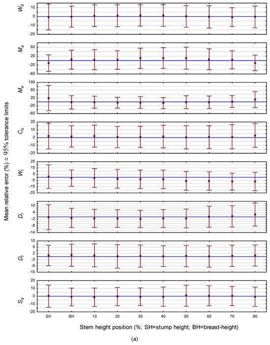
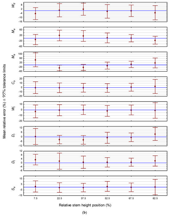
Figure 1.
(a) Predictive performance of the attribute-specific jack pine models: relative mean error and associated 95% tolerance intervals by stem height position. (b) Predictive performance of the attribute-specific red pine models: relative mean error and associated 95% tolerance intervals by stem height position.
Although dependent on the error threshold tolerance of the end-user, caution should be nevertheless exercised when using the Ma and Me prediction models for single tree forecasts for either species, particularly at the lower relative stem height positions. Alternatively, however, the mean errors arising from a minimum of 10 future projections for these two attributes of either species would be generally acceptable, i.e., mean prediction errors of less than ±13% and ±15% for Me and Ma, respectively, across all stem positions, for the jack pine models (Table 4), and mean prediction errors of less than ±14% and ±25% for Ma and Me, respectively, across all stem positions for the red pine models (Table 5). Consequently, deploying the Me and Ma equations to provide sample-based mean estimates for a group of trees rather than deploying them to yield individual tree predictions would be advisable.
The predictive ability of the models for estimating the end-point attribute value was also assessed graphically. Specifically, for all cross-sectional disks within the validation data subset which had a cambial age termination value that matched the last annual ring within a given relative height class, attribute-specific 95% predictive error tolerance intervals were calculated for each species and graphically presented (Figure 2). As illustrated for jack pine in Figure 2a, the intervals were relatively stable across all 10 relative stem height positions, although there was slight increase in interval width at the stump section for five of the eight attributes (i.e., Me, Co, Wt, Dr and Sa). Likewise, as illustrated for red pine in Figure 2b, the intervals were also relatively stable across all six relative stem height classes. However, contrary to the inference for jack pine, the interval range was slightly greater at the upper most stem position for all attributes but Dt. Similarly, intervals at the lowest stem region revealed a slight overestimation for Wd, Co, Wt and Dt. Overall, the magnitudes of the attribute-specific end-point biases were generally lower than those observed across all cambial ages for both jack pine (cf., Figure 1a and Figure 2a) and red pine (cf., Figure 1b and Figure 2b).
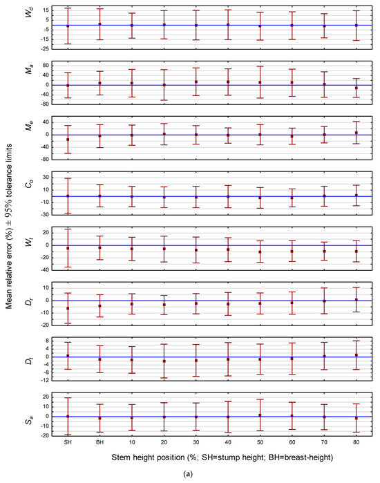
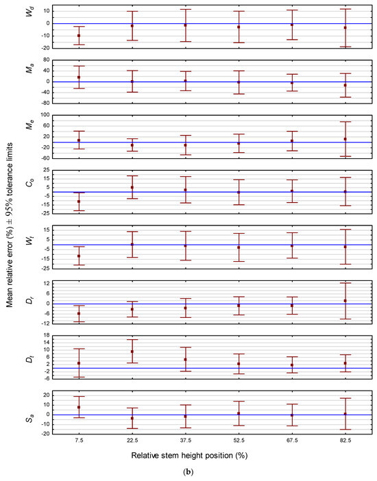
Figure 2.
(a) End-point predictive performance of the attribute-specific jack pine models: relative mean error and associated 95% tolerance intervals by stem height position. (b) End-point predictive performance of the attribute-specific red pine models: relative mean error and associated 95% tolerance intervals by stem height position.
3.3. Species-Specific Equation Suites: Full Data Set Parameterizations
In order to yield a set of deployable functional forms reflective of the full data sets, the final model specifications for each attribute were reparameterized by employing all of the observations within the respective species-specific data set. Table 6 and Table 7 provides the resultant parameter estimates and associated regression statistics for the final model forms for jack pine and red pine, respectively. Overall, the parameter values were similar in terms of their sign and magnitude to those estimated using the calibration data subset for all attributes irrespective of species (cf. Table 2 with Table 6 for jack pine and Table 3 with Table 7 for red pine). One notable exception, however, was the retransformed intercept coefficient for Wd specific to red pine. Contrasting the values for the standard error of estimate and the index-of-fit metric for the species-specific equations parameterized by the calibration and the full data sets revealed that the magnitude of the regression statistics were also comparable (i.e., comparing attribute-specific values for index-of-fit and the standard error of estimates in Table 2 with those in Table 6 for jack pine, and in Table 3 with those in Table 7 for red pine). Implicitly, these results suggest that the calibration data subsets arising from the deployed data stratification approach did not comprise model parameterization efforts given the approximate equivalence of the magnitude and polarity of the parameter estimates, and overall lack-of-fit measures. To exemplify these resultant functional forms within the context of the full data sets, the species-specific predicted attribute trajectories along with the corresponding observed trajectories at each height position are collectively presented in Figure 3a for jack pine and Figure 3b for red pine.
Table 6.
Parameter estimates and associated statistics for the attribute-specific hierarchical mixed-effects models (Equation (5)) for jack pine parameterized by employing the full data set.
Table 7.
Parameter estimates and associated statistics for the attribute-specific hierarchical mixed-effects models (Equation (5)) for red pine parameterized by employing the full data set.
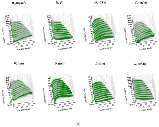
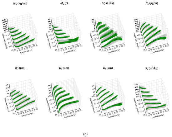
Figure 3.
(a) Scatterplots of individual-tree predicted attribute trajectories (green solid squares; Table 6) and corresponding observed trajectories (tan coloured open squares; full data set) are collectively presented for each jack pine attribute by relative height class and fixed-stem position (stump and breast-height (BH)). (b) Scatterplots of individual-tree predicted attribute trajectories (green solid squares; Table 7) and corresponding observed trajectories (tan coloured open squares; full data set) are collectively presented for each red pine attribute by relative height class.
4. Discussion
4.1. Cross-Validation Method Deployed and Resultant Explanatory Ability and Predictive Performance of the Parameterized Whole-Stem Wood Quality Attribute Prediction Models
Analytically, this study deployed an a priori strategic data splitting technique in order to reduce the presence of significant serial correlation within the attribute sequences before specifying and parameterizing the models. Essentially, this block cross-validation-like approach identified the inherent serial correlation pattern within the cross-sectional temporal attribute sequences and used that knowledge to remove sufficient consecutive observations so as to reduce its presence without compromising model specification efforts (sensu [25,26]). More specifically, the method consisted of assessing the magnitude and pattern of the serial correlation using partial autocorrelation coefficients (i.e., determining the number of significant correlated temporal lags). Given the resultant lag patterns observed, all attribute sequences were then systematically reduced through the removal of two-observation-long blocks sequentially along each attribute sequence (e.g., removal of the 3rd, 4th and 6th, 7th, and so forth, cohort-age-specific values), yielding an assumed uncorrelated temporal sequence consisting of the remaining 2nd, 5th, 8th, and so forth, cohort-age-specific values. These sequences, when collectively combined by species and attribute, comprised the data subsets used to specify and parameterize the models. The removed cohort-age-specific values were then deployed in the creation of corresponding validation data subsets. Although this approach did not entirely eliminate the presence of serial correlation, it did substantially decrease its occurrence as reflected by its reduced presence among first-level residuals following model parameterization (e.g., Table 4 and Table 5). Noteworthy tenets to this approach include the following: (1) although the degree of data splitting is largely dependent on the serial correlation pattern observed within the temporal sequences, attention must also be focused on potential specification errors arising from over removal (e.g., in this study, two out of every three consecutive age-cohort values within each attribute sequence required removal given the 2-lag serial correlative structure observed (Table A1)) and (2) block-type cross-valuation-like approaches when applied to time series data structures do not yield truly independent validation data subsets, and thus reported predictive performance measures may be inflated. Parametric-based approaches such as mixed-effects regression analyses with assumed covariance structures (e.g., first-order autoregressive) or autoregressive moving average modeling techniques may have also been viable alternative approaches to the data splitting method deployed in this study, in terms of addressing the inherent serial correlation structure within the attribute sequences (e.g., [32]). However statistical assumptions regarding error structures and autocorrelative relationships are required with deployment of these alternative methods and, as such, may not entirely eliminate data-dependent effects (sensu [25]).
Generally, quantifying the inherent spatiotemporal attribute development patterns at the whole-stem level along with identifying their underlying physiological, environmental, biophysical and silvicultural-induced determinates remains an active and increasingly important area of investigation within the wood quality modeling and carbon accounting communities. Such research is an essential but challenging prerequisite to addressing end-product and carbon-retainment forest management objectives. Drew et al. [33], in a comprehensive review of wood quality modeling efforts, identified a number of successful empirical-based modeling approaches that have been deployed in quantifying whole-stem pith-to-bark attribute variability. Although such approaches have been largely concentrated on coniferous species and focused on describing wood density, microfibril angle, and modulus of elasticity development patterns and variability, hierarchical mixed-effects and logarithmic-based models were considered to be among the most promising (see Table 1 in [33]). Generalized additive mixed models where also found to be successful in terms of identifying and differentiating the underlying intrinsic and extrinsic determinates controlling attribute variation.
In this study, the whole-stem cumulative attribute developmental patterns for both studied pine species were quantified deploying a hierarchical mixed-effects modeling approach. The resultant models exhibited an adequate level of overall explanatory power and predictive accuracy as derived from the statistical-based cross-validation analysis. The jack pine equations explained 46, 66, 74, 63, 59, 72, 42 and 48% of the variation in Wd, Ma, Me, Co, Wt, Dr, Dt and Sa, respectively, whereas the red pine equations explained 50, 71, 31, 83, 72, 78, 56 and 71% of the variation in Wd, Ma, Me, Co, Wt, Dr, Dt and Sa, respectively. Although not consequentially different between the species, the equations for red pine were slightly superior, i.e., explaining 31% to 83% of the variation (mean of 64%) versus 42% to 74% of the variation (mean of 59%) for jack pine. In terms of predictive ability, the relative tolerance error limits across the 10 relative stem height positions for jack pine ranged from a minimum of ±11% to a maximum of ±14% (stump) for Wd, ±35% to ±49% (stump) for Ma, ±28% to ±65% (stump) for Me, ±14% to ±16% (stump) for Co, ±13% to ±19% (stump) for Wt, ±8% to ±11% (stump) for Dr, ±6% to ±7% for Dt, and from ±11% to ±14% for Sa. For red pine, the relative tolerance error limits ranged from ±8% to ±10% for Wd, ±26% to ±39% for Ma, ±26% to ±64% (stump) for Me, ±9% to ±16% for Co, ±9% to ±14% for Wt, ±6% to ±11% for Dr, ±4% to ±8% for Dt, and from ±8% to ±14% for Sa. However, the magnitude of tolerance intervals for prediction error did vary by stem position, more so for jack pine than for red pine. Specifically, predictions at the stump position for Wd, Ma, Me, Co, and Wt for jack pine and Ma for red pine exhibited the largest tolerance interval widths, suggesting a consistent pattern of decreased predictive ability at the lowest stem position. Although variation in fibre alignments could affect attribute estimates when determined via Silviscan-based analyses, and hence may be potentially partially responsible for this observed pattern, lower model performance for the stump region is not uncommon with attribute prediction models. For example, wood formation at the base of the stem can be influenced by mechanical forces such as those arising from wind-induced tree swaying. This can result in greater attribute variation across the cross-section due to differences in wood formation patterns (e.g., [34]). Thus, potentially yielding relatively lower levels of predictive precision when quantified through regression-based modeling methods which do not account for wood-type variation (e.g., compression and reaction wood types).
The three-level hierarchical mixed-effects whole-tree attribute models developed for jack pine and red pine in this study were similar in their explanatory power and predictive accuracy as those previously developed using a two-level hierarchical mixed-effects spatial-invariant model specification for black spruce and jack pine ([7,9], respectively). For example, contrasting the proportion of variation described by the equations among the species-specific models suggested approximate equivalency: (1) three-level models for jack pine developed in this study explained 62, 55, 71, 71, 71 49, 16 and 64% of the variation in Wd, Ma, Me, Co, Wt, Dr, Dt and Sa, respectively, at the breast-height position (Table 4) versus 60, 55, 71, 75, 71, 49, 38 and 66% of the variation in Wd, Ma, Me, Co, Wt, Dr, Dt and Sa, respectively, for the two-level jack pine models (Table 3 in [9]), and (2) and 74, 72, 74, 62, 63, 88, 70 and 61% of the variation in Wd, Ma, Me, Co, Wt, Dr, Dt and Sa, respectively, for the two-level black spruce models (Table 3 in [7]). Likewise, contrasting the among of variation explained for the three-level red pine models (i.e., 61, 51, 82, 81, 72, 76, 72 and 68% of the variation in Wd, Ma, Me, Co, Wt, Dr, Dt and Sa, respectively, at the 7.5% relative height position (Table 5)) with that for the two-level jack pine and black spruce models, revealed a similar range for explanatory abilities among the species-specific models. In terms of prediction ability, contrasting the breast-height positional results among the species-specific models also suggested approximate equivalency. Specifically, examining the tolerance intervals for relative error at the breast-height position produced by the three-level hierarchical jack pine models with respect to those produced from the previous developed spatially invariant (breast-height position) two-level hierarchical models, revealed similar predictive abilities, i.e., 95% of all future relative errors for Wd, Ma, Me, Co, Wt, Dr, Dt and Sa were bounded within a ±12, ±42, ±34, ±14, ±13, ±9, ±7 and ±11% interval, respectively, when using the three-level model specifications (i.e., values reported for breast-height; Table 4) versus the ±12, ±42, ±35, ±12, ±13, ±9, ±5 and ±11% intervals for Wd, Ma, Me, Co, Wt, Dr, Dt and Sa, respectively, generated using the two-level model specifications (Table 3 in [9]). The tolerance intervals for the three-level hierarchical models for red pine were also comparable to those for jack pine when predicting approximate breast-height estimates for 7 of the 8 attributes (Me being the expectation), i.e., 95% of all future relative errors for Wd, Ma, Me, Co, Wt, Dr, Dt and Sa were bounded within a ±9, ±37, ±64, ±14, ±12, ±11, ±5 and ±10% interval (i.e., values reported at the 7.5% relative height position; Table 5).
Notably, across the three conifers for which such comparable attribute equations and statistics exist, the predictive performance metrics suggested a similar differentiation among attributes (Table 4 and Table 5 in this study for jack pine and red pine, respectively, for the three-level models; Table 3 in [7] for the two-level black spruce models; and Table 3 in [9] for the two-level jack pine models): Wd, Co, Wt, Dr, Dt and Sa >> Ma and Me. The consistent attribute ranking in terms of predictive performance presents an inherent challenge when attempting to model the development patterns of this latter set of key end-product-related determinates, i.e., microfibril angle and the modulus of elasticity. Examination of the degree of relative variation among these attributes within the Silviscan data sets for black spruce (Table 1 in [7], jack pine (Table S2a) and red pine (Table S2b), as quantified by the coefficient of variation, suggest that these attributes are intrinsically more variable than the other six attributes examined.
According to the predicted trajectories as displayed within the context of the full data (i.e., Figure 3a for jack pine and Figure 3b for red pine), the trajectories were in general concordance with the observed trajectories in terms of mirroring the overall nonlinear polymorphic temporal trends within the cross-sectional disks, irrespective of height position, attribute or species. Similar to the validation assessment results, the least degree of concordance was observed within the wood density, microfibril angle, modulus of elasticity and fibre coarseness trajectories, particularly within the cross-sectional disks located within the lower bole region. Although predicted spatiotemporal development patterns were similar between the species irrespective of attribute, at a given height position, jack pine exhibited a greater degree of nonlinearity in the Wd and Dt trajectories, whereas red pine exhibited a greater degree of nonlinearity in the Ma, Me, Co, Wt, Dr, and Sa trajectories. However, for both species and irrespective of attribute, the greatest degree of nonlinearity occurred before a cambial age of approximately 30 years.
Overall, the predicted and observed trajectories throughout the stem of both species were similar to those reported for jack pine at the breast-height position [9]. Likewise, the significance of the tree-level size variable (diameter at breast-height) introduced at the third hierarchical level across all the attributes (i.e., Table 2 and Table 3) reconfirms and expands the size-dependence inference previously reported for black spruce and jack pine with respect to breast-height-based cumulative attribute developmental trajectories ([7,9], respectively). Although not shown, size-dependent attribute trajectory differences for the models parameterized using the entire data sets (Table 6 and Table 7) were most evident at the lower relative stem height positions (<30%). For example for red pine, within the stump height to breast-height region, wood density and the modulus of elasticity exhibited an inversely correlative relationship with tree size, whereas microfibril angle exhibited a directly correlative relationship. This suggests that the solid wood producing potential of logs extracted from the lower stem of larger diameter trees would yield lower quality wood products relative to such logs extracted from smaller diameter trees.
In summary, based on the graphical assessments and statistical metrics related to residual error patterns, goodness-of-fit, lack-of-fit and predictive performance, which were devoid of evidence suggesting the presence of systematic biases, misspecification or unacceptable predictive ability, the resultant parameterized models were considered unbiased predictors and correctly specified quantitative descriptors of the spatiotemporal whole-stem cumulative attribute developmental patterns, for these two pine species.
4.2. Analytical Approaches to Quantifying Whole-Stem Attribute Distributions: Annual Ring-Specific Prediction Models and Composite Modeling Approaches
Historically, the analytical approaches utilized in the quantification of within-stem attribute variation arising from innovative advancements in attribute determination methods, such as X-ray densitometry, Silviscan and near-infrared spectroscopy, have included descriptive graphical interpolation methods (e.g., [6,10,35,36]) and empirical prediction modeling (e.g., [37,38,39,40]). With respect to prediction modeling, one of the earlier attempts to develop within-stem wood attribute prediction models for conifers were those of Ikonen et al. [38]. They developed a non-spatial empirical ring-based model for estimating wood density within the stems of Scots pine (Pinus sylvestris L.) and Norway spruce (Picea abies (L.) Karst.) using early wood percentage indirectly estimated from ring width and cambial age as explanatory variables. Their models explained approximately 40% of the variation in wood density. They also integrated the models within a process-based growth and yield model in order to simulate how site occupancy regulation (thinning) and varying climate change conditions could affect wood density and its within-stem distribution at rotation age. Development of spatially explicit models followed somewhat later, as exemplified by Deng et al. [39], who specified and parameterized a mixed-effects regression model for predicting wood density variation within Masson pine (Pinus massoniana Lamb.) stems. Their model utilized tree age, tree size (diameter at breast-height) and relative stem height position as independent variables in order to predict cross-sectional mean wood density at any stem position within a tree of given age and size. The resultant model explained approximately 91% of the variation in mean cross-sectional wood density. Furthermore, in order to predict specific gravity at the annual ring level throughout the entire stem of loblolly pine trees, Dahlen et al. [41] parameterized a fixed-effects whole-tree regression model specification deploying cambial age and stem height as independent variables. The resultant model was able to describe approximately 55% of the variation in the dependent variable and, when combined with a taper equation, was able to generate interpolated whole-tree property maps for this specific attribute and species. Notably, the addition of annual ring width to potentially account for growth increases arising from silvicultural treatments such as thinning within the model specification did not consequentially improve the overall explanatory ability of the resultant prediction model. Similarly, for the same species and deploying a similar model specification inclusive of positional effects (stem height), Dahlen et al. [42] presented a spatially explicit model for predicting annual ring-specific tracheid width. The resultant model, which described 57% of the variation in tracheid width, was then used to project 25-year section-specific rotational estimates and associated property maps under an assortment of timber production scenarios.
More generally, individual annual ring attribute values can vary dramatically within cross-sectional sequences due to intrinsic ontogenetic wood formation processes and a broad array of extrinsic naturogenic and anthropogenic influences (e.g., annual variation in growing conditions, silvicultural treatment effects, climate change). Variation in attribute-specific phenotypic plasticity arising in response to external stimuli can also be a confounding source of unexplained variation when quantifying attribute developmental patterns. For example, development of dense compression wood on the leeward side versus formation of less dense reaction wood on the windward side within lower stem regions is a common occurrence within trees subjected to high wind-induced forces (e.g., [34]). Consequently, development of annual ring-specific attribute prediction models that can deliver a high level of explanatory power and predictive ability has been challenging.
In an attempt to minimize such variation when quantifying attribute development patterns within coniferous forest tree species, mean-based approaches have also been advanced. These have included the cross-sectional mean metric utilized by Deng et al. [39] and the cumulative annual ring-area-weighted moving average metric utilized by Newton [7,8,9]. This latter metric is a measure of central tendency that is reflective of an attribute’s historical development pattern. Although inherent variability is reduced with the deployment of such a metric, the resultant attribute development trajectories can retain their complex polymorphic-like nonlinear curve shapes, which can be analytically challenging to quantify (e.g., see Figures 1 and 4 in [7]). However, the ability of the Hoerl model to describe such a wide array of complex unimodal nonlinear trends, as exemplified by Daniel and Wood (Figure 3.4 in [43]), renders it an analytical consideration when modeling fibre attribute trajectories. Even though the model has not been widely used in forestry, it has been successfully utilized in the development of a generic diameter inside a bark prediction equation [44], a diameter growth equation [45], and by the author in the development of spatial-invariant attribute models for black spruce and jack pine (i.e., [7,9], respectively). Such success bodes well for its continued consideration when modeling attribute development and tree growth trajectories.
Furthermore, the deployment of the cumulative annual ring-area-weighted moving average metric within the context of the tri-level hierarchical equations developed in this study provides a unique perspective in terms of end-product potential. Specifically, this composite metric for a given attribute reflects the collective end-product potential at a given cambial age and stem location for a tree of specified size, when product-specific design and associate grading specifications are known. The extraction of solid wood products is usually spatially invariant and dimensional-dependent with limited grade class delineation when sawlogs are processed by conventional SPF-based sawmilling protocols. Although visual grading is of utility in terms of classifying dimensional lumber into grade classes (e.g., Select Structural, No. 1, No. 2, No. 3, and Economy; [46]) when using such attributes as knot size, grain deviation, degree of wane and presence of decay, more precise spatial-based zonal differentiation of internal wood fibre attributes remains elusive. By contrast, however, machine stress-rated (MSR) grading guidelines for SPF lumber include specific wood attribute thresholds [47], i.e., wood density and static modulus of elasticity ranges by grade class. Although the assumption of absolute equivalency between Silviscan-based dynamic modulus of elasticity estimates within standing trees and the static modulus of elasticity within extracted dimensional lumber is not fully tenable (sensu [48]), an approximate inferential classification framework system can nevertheless be derived based on the Silviscan-based attribute estimates predicted by the equations presented in this study. Hence, by deploying the cumulative attribute moving average estimates for wood density and the modulus of elasticity of a given standing tree or extracted log, the grade class of potentially extractable lumber can be approximated. This ability to generate rotational end-product potentials at the log, tree and stand levels given stem position-specific attribute predictions enables inferences to be drawn with respect to end-product outcomes for the entire harvestable stem. Exemplifications of such will be presented in the companion contribution (i.e., [14]).
4.3. Biomechanical Linkages and Potential Consequences for Whole-Stem Attribute Modeling
The plasticity of excurrent forest tree species in terms of adjusting their morphology and allometry to accommodate environment-induced stresses enables them to successfully adapt to resource-limiting and space-restricted growing environments. This plasticity not only includes changes in height–diameter allometry to accommodate gravity-induced self-loading forces, but also extends to changes in the temporal and spatial developmental patterns of within-stem fibre attributes in order to accommodate wind-induced bending and twisting forces [49].
These biomechanical adaptions yield flexible tree stems that can tolerate an impressive degree of stress and strain before stem breakage or uprooting occurs. Generally, increasing buttresses within the lower stem region partially mitigates the effect of gravitational forces acting on the root system and improves overall stability. For example, as the ratio of the breast-height diameter to root collar diameter decreases, resistance to snapping and uprooting increases (sensu [50]). Likewise, decreasing stiffness with increasing height increases stem flexibility, which allows trees to systematically dissipate wind-induced crown-based drag forces [51]. Although the likelihood of structural failure or uprooting during high velocity wind events is reduced, the probability of physical interaction among neighboring trees increases. The resultant frictional interactions within forest stands can lead to crown damage and associated foliar biomass losses (crown shyness), which may ultimately result in tree mortality patterns analogous to those observed during the self-thinning phase (i.e., asymmetric size-dependent mortality). Spatially, the stem region subjected to the most intense wind-induced bending forces is located slightly above the buttressed region (e.g., [50]). Although the probability of breakage is relatively high within this region, changes in the anatomical characteristics of xylem tissue within the stem may confer an advantage in terms of lowering the likelihood of mechanically induced stem failure.
The unique characteristics of this study in terms of the presentation and quantification of whole-stem attribute distribution patterns for two intensively managed coniferous species provide an opportunity to examine possible biomechanical linkages, and how they may be potentially leveraged to improve future whole-stem attribute models. For example, examination of the vertical distribution of the attributes that underlie the structural integrity of standing coniferous stems revealed a consistent vertical distributional pattern for the studied jack pine and red pine trees (Tables S2a and S2b, respectively): (1) wood density decreased linearly with increasing height; (2) modulus of elasticity increased from the stump to a relative height of approximately 30%, and thereafter linearly declined with increasing stem height; and (3) the highest wood density and modulus of elasticity values occurred within the 20%–40% relative height region. Similarly, the whole-stem model-based projections for these species, as exemplified in the companion contribution, were also congruent with such trends (i.e., [14]). Other studies, such as that of Waghorn [52], who examined the longitudinal (vertical) variation in the dynamic modulus of elasticity within radiata pine (Pinus radiata D. Don) trees across a gradient of initial spacings and a mixture of genotypes, observed similar patterns: stiffness values increased from the stump upward, attaining maxima across the 15%–45% relative height range (maximizing on average at the relative height of 27%), and then declined systematically with increasing stem height until the stem apex was reached. These longitudinal stiffness trends were consistent across all five initial spacing treatments and five genotypes examined. Likewise, based on in-forest elasticity–stem height measurements for standing Sitka spruce (Picea sitchensis (Bong.)) trees, Brüchert and Gardiner [51] revealed a nonlinear declining trend with increasing stem height (e.g., as reflected by a second-degree polymorphic regression equation specification).
Conceptually, the concentration of maximum stem stiffness within the lower stem region is suggestive of a morphological plastic response for mitigating the effects of gravitational and wind-induced bending and twisting forces. Examination of the distribution of the density-specific stiffness ratio, which has also been used to quantify a tree stem’s ability to withstand such stresses (sensu [53]), also revealed its maximization within the 20%–40% relative height region when calculated for the pine species examined in this study (i.e., Me/Wd ratios as calculated from the observed height-specific mean attribute values as presented in Table S2a for jack pine and Table S2b for red pine). Although these empirical exemplifications employed the observed sample-based mean values, the attribute equations could likewise be of utility in biomechanical and allometric scaling analyses given their ability to generate longitudinal density-specific stiffness profiles for the entire stem. Size-dependent effects on within-stem density-specific stiffness profiles could also be assessed given the tertiary nature of the attribute model specifications presented. Tangentially, it is also worthwhile to note that for a number of excurrent boreal coniferous species (e.g., balsam fir (Abies balsamea (L.) Mill.), black spruce and white spruce (Picea glauca (Moench) Voss)), the 20%–40% relative stem height region is also the point where the center of gravity of the standing stem occurs (i.e., 30% relative height position [54]). According to the associated paracone stem profile model developed by Forslund [55], approximately 50% of a stem’s volume would be expected to be concentrated within this lower stem region. Thus, combining this volumetric inference with a lower stem stiffness prediction could yield a partial estimate of end-product potential of standing trees. For example, deploying the sample values for wood density and the modulus of elasticity for jack pine and red pine for the lower bole region (≤≈30% relative height; Tables S2a and S2b, respectively) infers that approximately 50% of the stem mass (volume) would be conducive to the production of solid wood end-products. Specifically, given mean wood density and stiffness values are 432 kg/m3 and 12.4 GPa, respectively, for jack pine, and 407 kg/m3 and 11.8 GPa, respectively, for red pine, suggests that at least 50% of the harvested stem volume would be capable of yielding dimension lumber products upon sawmill processing (sensu [47]).
Acknowledging plausible environmental–biomechanical relationships that may influence attribute spatial distributions within tree stems may be of utility when considering new covariates for potential inclusion in future whole-stem attribute prediction models. For example, incorporating surrogate variables that are reflective of environmental causal-based determinates such as gravitational and wind-induced forces that underlie longitudinal stiffness distributions (e.g., slenderness ratio (height–diameter ratio)), may improve predictive performance. Appreciating potential linkages between within-stem attribute patterns and applicable biomechanical axioms may be advantageous when developing whole-stem attribute prediction models in the future, particularly in terms of reducing the degree of empiricism, increasing model generality, and potentially establishing functional linkages between tree-level within-stem attribute distributions and stand-level environment-based determinates.
4.4. Advancing Whole-Tree Attribute Modeling and Evolving Research Opportunities
Analytically, the ability of the tertiary-level hierarchical mixed modeling framework to describe temporal attribute developmental patterns throughout the entire main stem of individual trees by size class provides an inferential framework for evaluating end-product potential at the whole-tree level. For example, deploying the resultant models within pre-harvest end-product forecasting surveys, post-harvest fibre segregation operations or crop planning decision-support systems enables the estimation of log-specific end-product potential throughout the entire vertical (height) and horizontal (diameter) stand-level structural dimensions. Although the previously developed two-level hierarchical models were of consequential utility in estimating attributes at breast-height and inferring associated end-product potential for the first-order extractable log within a tree of given size (e.g., [9]), the three-level attribute models provide a whole-stem and hence multi-log description of rotational end-product potential for a tree of specified size. Operationally, this additional knowledge enriches and improves end-product forecasting in terms of providing the foundation for optimal log segregation and allocation decision making, hence potentially yielding logistical and economic efficiency gains within the upper portion of the forest products supply chains for these species.
Quantifying size-dependent developmental trends of commercially relevant fibre attributes throughout the entire stem profile of excurrent coniferous species is an analytically challenging endeavor. Nevertheless, such relationships are essential prerequisites to projecting end-product potentials from pre-harvest forest inventory surveys, addressing value-based crop planning objectives and spatial delineation of extractable end-products using resultant whole-stem attribute property maps. This enables the optimization of log segregation and allocation decision making at the time of harvest, e.g., differentiating logs according to their end-product potential (e.g., dimensional lumber derivatives versus pulp and paper products) and directing them to the most applicable conversion centre (e.g., sawmill or pulp and paper mills). Furthermore, when attribute equations are combined with traditional inventory metrics or incorporated within crop planning models, the generated stand level estimates can be used to inform forest management planning decision making (e.g., determining optimal rotation ages or density management regimes that maximize the production of solid wood end-products; sensu [14]). The ability to estimate the type, quantity and quality of harvestable wood products extracted from the entire merchantable stem of jack pine and red pine trees may also be of consequential utility when evaluating competing crop plans on their long-term carbon storage potential (sensu [56]).
5. Conclusions
The ability to address value-based forest management objectives is partially dependent on the access to allocation, segregation and crop planning tools that can provide tree-level end-product estimates. Given that the type and quality of end-products extracted from individual trees are intrinsically related to internal wood quality attributes, this study formulated, parameterized and validated a suite of spatiotemporal whole-stem prediction models for estimating a suite of such attributes at any given stem height position for two intensely managed coniferous species, jack pine and red pine. These models extend the previously developed spatially invariant (breast-height-only) models by enabling spatially explicit forecasting of end-product potential throughout the entire tree stem. Analytically, the resultant species-specific equation suites generated unbiased and relatively precise whole-stem predictions of wood density, microfibril angle, modulus of elasticity, fibre coarseness, tracheid wall thickness, tracheid radial diameter, tracheid tangential diameter and specific surface area. These modeled attributes were considered among the most important xylem-based determinates underlying end-product potential. Consequently, the resultant relationships could find utility in generating pre-harvest and post-harvest end-product forecasts, enhancing crop planning decision-support models, and possibly addressing shortcomings in existing inventory-based carbon sequestration and retainment accounting models. Furthermore, the inferred allometric and biomechanical linkages with respect to environment-based determinates (gravitational and wind-induced forces), which affect within-stem wood density and stiffness distributions, suggest more causal-driven specifications are possible when developing future whole-stem wood attribute models.
Supplementary Materials
The following supporting information can be downloaded at: https://www.mdpi.com/article/10.3390/f14112211/s1, This file includes four tables providing species-specific descriptive statistical summaries for the deployed sample data sets, i.e., stem-based mensurational and attribute characteristics by relative height sampling position. Note, the specific contents of each table are self-evident by its title: (1) Table S1a was entitled “Cross-sectional position-based mensurational metrics for the 610 jack pine disk samples”; (2) Table S1b was entitled “Cross-sectional position-based mensurational metrics for the 223 red pine disk samples”; (3) Table S2a was entitled “Descriptive statistical summary of the jack pine fibre attributes by cross-sectional relative height sampling position”; and (4) Table S2b was entitled “Descriptive statistical summary of the red pine fibre attributes by cross-sectional relative height sampling position”.
Funding
This research was funded internally by the author’s employer, the Canadian Forest Service.
Acknowledgments
The author expresses his appreciation to: (1) Mike Laporte (Retired) from the Great Lakes Forestry Centre (GLFC), Canadian Forest Service (CFS), Natural Resources Canada (NRCan) and Gordon Brand at the GLFC, CFS, NRCan, for field and laboratory data acquisition support; (2) logging machine operators and planning staff from Thomas Woods Development Inc., Bruce Mines, ON, Canada, for felling and sectioning the 54 red pine sample trees; (3) Tessie Tong and Nelson Uy at FPInnovations, Vancouver, BC for completing the SilviScan-3 analysis; (4) the CFS for internal fiscal support; and (5) three anonymous peer reviewers and the Forests editors for their constructive comments and suggestions, which ultimately yielded an improved contribution.
Conflicts of Interest
The author declares no conflict of interest. The funders had no role in the design of the study; in the collection, analyses, or interpretation of data; in the writing of the manuscript; or in the decision to publish the results.
Appendix A
Table A1.
Preliminary autocorrelation analysis: number (n) and percentage (%) of cross-sectional cumulative moving average attribute sequences exhibiting significant (p ≤ 0.05) autocorrelation by attribute, lag and species as determined by the partial autocorrelation coefficients.
Table A1.
Preliminary autocorrelation analysis: number (n) and percentage (%) of cross-sectional cumulative moving average attribute sequences exhibiting significant (p ≤ 0.05) autocorrelation by attribute, lag and species as determined by the partial autocorrelation coefficients.
| Species | Lag (Year) | Attribute a | |||||||||||||||
|---|---|---|---|---|---|---|---|---|---|---|---|---|---|---|---|---|---|
| Wd | Ma | Me | Co | Wt | Dr | Dt | Sa | ||||||||||
| n | % | n | % | n | % | n | % | n | % | n | % | n | % | n | % | ||
| Jack | 1 | 591 | 96.9 | 610 | 100.0 | 610 | 100.0 | 604 | 99.0 | 604 | 99.0 | 609 | 99.8 | 534 | 87.5 | 597 | 97.9 |
| pine | 2 | 119 | 19.5 | 13 | 2.1 | 13 | 2.1 | 179 | 29.3 | 129 | 21.1 | 80 | 13.1 | 92 | 15.1 | 160 | 26.2 |
| (n = 610) | 3 | 37 | 6.1 | 0 | 0.0 | 1 | 0.2 | 17 | 2.8 | 14 | 2.3 | 7 | 1.1 | 16 | 2.6 | 35 | 5.7 |
| Red | 1 | 215 | 96.4 | 222 | 99.6 | 221 | 99.1 | 223 | 100.0 | 220 | 98.7 | 221 | 99.1 | 223 | 100.0 | 220 | 98.7 |
| pine | 2 | 41 | 18.4 | 0 | 0.0 | 3 | 1.3 | 21 | 9.4 | 19 | 8.5 | 5 | 2.2 | 21 | 9.4 | 27 | 12.1 |
| (n = 223) | 3 | 7 | 3.1 | 0 | 0.0 | 0 | 0.0 | 5 | 2.2 | 7 | 3.1 | 2 | 0.9 | 7 | 3.1 | 12 | 5.4 |
a Wd, Ma, Me, Co, Wt, Dr, Dt and Sa denote wood density, microfibril angle, modulus of elasticity, fibre coarseness, tracheid wall thickness, tracheid radial diameter, tracheid tangential diameter and specific surface area, respectively.
Appendix B


Figure A1.
Attribute-specific observed versus predicted value scatterplots for jack pine by relative stem height class: (a) wood density; (b) microfibril angle; (c) modulus of elasticity; (d) fibre coarseness; (e) tracheid wall thickness; (f) tracheid radial diameter; (g) tracheid tangential diameter; and (h) specific surface area. Notes: (1) diagonal solid red line denotes the line of equivalence (y = x); and (2) BH denotes breast-height (1.3 m).


Figure A2.
Attribute-specific observed versus predicted value scatterplots for red pine by relative stem height class: (a) wood density; (b) microfibril angle; (c) modulus of elasticity; (d) fibre coarseness; (e) tracheid wall thickness; (f) tracheid radial diameter; (g) tracheid tangential diameter; and (h) specific surface area. Note, the diagonal solid red line denotes the line of equivalence (y = x).
References
- Rowe, J.S. Forest Regions of Canada; Publication No. 1300; Government of Canada, Department of Environment, Canadian Forestry Service: Ottawa, ON, Canada, 1972.
- Zhang, S.Y.; Koubaa, A. Softwoods of Eastern Canada: Their Silvics, Characteristics, Manufacturing and End-Uses; Special Publication SP-526E; FPInnovations: Quebec City, QC, Canada, 2008. [Google Scholar]
- Walker, W.S.; Gorelik, S.R.; Cook-Patton, S.C.; Baccini, A.; Farina, M.K.; Solvik, K.K.; Ellis, P.W.; Sanderman, J.; Houghton, R.A.; Leavitt, S.M.; et al. The global potential for increased storage of carbon on land. Proc. Natl. Acad. Sci. USA 2022, 119, e2111312119. [Google Scholar] [CrossRef] [PubMed]
- Li, L.; Wei, X.; Zhao, J.; Hayes, D.; Daigneault, A.; Weiskittel, A.; Kizha, A.R.; O’Neill, S.R. Technological advancement expands carbon storage in harvested wood products in Maine, USA. Biomass Bioenergy 2022, 161, 106457. [Google Scholar] [CrossRef]
- Intergovernmental Panel on Climate Change (IPCC). Agriculture, Forestry, and Other Land Uses (AFOLU). In Climate Change 2022: Mitigation of Climate Change, the Working Group III Contribution; Chapter 7, Sixth Assessment Report; IPCC: Geneva, Switzerland, 2022. [Google Scholar]
- Defo, M. SilviScan-3 A Revolutionary Technology for High-Speed Wood Microstructure and Properties Analysis; Midis de al Foresterie; UQAT. 2008. Available online: http://chaireafd.uqat.ca/midiForesterie/pdf/20080422PresentationMauriceDefo.pdf (accessed on 1 October 2018).
- Newton, P.F. Quantifying size-dependent developmental trajectories of commercial-relevant fibre attributes within maturing black spruce plantations employing hierarchical linear models. For. Ecol. Manag. 2016, 381, 1–16. [Google Scholar] [CrossRef][Green Version]
- Newton, P.F. Developmental trends of black spruce fibre attributes in maturing plantations. Int. J. For. Res. 2016, 2016, 7895289. [Google Scholar] [CrossRef]
- Newton, P.F. Wood quality attribute models and their utility when integrated into density management decision-support systems for boreal conifers. For. Ecol. Manag. 2019, 438, 267–284. [Google Scholar] [CrossRef]
- Schimleck, L.; Antony, F.; Mora, C.; Dahlen, J. Whole-tree tracheid property maps for loblolly pine at different ages. Wood Sci. Technol. 2020, 54, 683–701. [Google Scholar] [CrossRef]
- Defo, M.; Goodison, A.; Nelson, U. A method to map within-tree distribution of fibre properties using SilviScan-3 data. For. Chron. 2009, 85, 409–414. [Google Scholar] [CrossRef]
- Murphy, G.; Cown, D. Stand, stem and log segregation based on wood properties: A review. Scand. J. For. Res. 2015, 30, 757–770. [Google Scholar] [CrossRef]
- Raudenbush, S.W.; Bryk, A.S. Hierarchical Linear Models: Applications and Data Analysis Methods, 2nd ed.; Sage: Newbury Park, CA, USA, 2002. [Google Scholar]
- Newton, P.F. Potential Utility of whole-Stem Wood Quality Prediction Models for Jack Pine and red Pine in End-Product Forecasting and Crop Planning Decision-Making. Canadian Wood Fibre Centre, Canadian Forest Service, Natural Resources Canada, Sault Sainte Marie, ON, Canada. 2024; in preparation. [Google Scholar]
- Newton, P.F. An acoustical-based predictive modeling suite for estimating commercially-relevant wood fibre attributes within jack pine logs. Forests 2018, 9, 749. [Google Scholar] [CrossRef]
- Newton, P.F. Acoustic-based prediction of end-product-based fibre determinates within standing jack pine trees. Forests 2019, 10, 605. [Google Scholar] [CrossRef]
- Newton, P.F. Predictive relationships between acoustic velocity and wood quality attributes for red pine logs. For. Sci. 2017, 63, 504–517. [Google Scholar] [CrossRef]
- Newton, P.F. Acoustic-based non-destructive estimation of wood quality attributes within standing red pine trees. Forests 2018, 8, 380. [Google Scholar] [CrossRef]
- Evans, R. Rapid measurement of the transverse dimensions of tracheids in radial wood sections from Pinus radiata. Holzforschung 1994, 48, 168–172. [Google Scholar] [CrossRef]
- Evans, R.; Stuart, S.A.; Van Der Touw, J. Microfibril angle scanning of increment cores by X-ray diffractometry. Appita J. 1996, 49, 411–414. [Google Scholar]
- Evans, R. Wood stiffness by X-ray diffractometry. In Characterization of the Cellulosic Cell Wall; Stokke, D.D., Groom, L.H., Eds.; Wiley: Hoboken, NJ, USA, 2006; pp. 138–146. [Google Scholar] [CrossRef]
- Hoerl, A.E. Fitting curves to data. In Chemical Business Handbook; Perry, J.H., Ed.; McGraw-Hill: New York, NY, USA, 1954; pp. 55–77. [Google Scholar]
- Neter, J.; Wasserman, W.; Kutner, M.H. Applied Linear Statistical Models, 3rd ed.; Irwin: Boston, MA, USA, 1990. [Google Scholar]
- Gujarati, D.N. Essential of Econometrics, 3rd ed.; McGraw-Hill: New York, NY, USA, 2006. [Google Scholar]
- Roberts, D.R.; Bahn, V.; Ciuti, S.; Boyce, M.S.; Elith, J.; Guillera-Arroita, G.; Hauenstein, S.; Lahoz-Monfort, J.J.; Schröder, B.; Thuiller, W.; et al. Cross-validation strategies for data with temporal, spatial, hierarchical, or phylogenetic structure. Ecography 2017, 40, 913–929. [Google Scholar] [CrossRef]
- Yates, L.A.; Aandahl, Z.; Richards, S.A.; Brook, B.W. Cross validation for model selection: A review with examples from ecology. Ecol. Monogr. 2023, 93, e1557. [Google Scholar] [CrossRef]
- Raudenbush, S.W.; Bryk, A.S.; Cheong, Y.F.; Congdon, R. HLM 8 for Windows; Scientific Software International, Inc.: Skokie, IL, USA, 2019. [Google Scholar]
- Piñeiro, G.; Perelman, S.; Guerschman, J.P.; Paruelo, J.M. How to evaluate models: Observed vs. predicted or predicted vs. observed? Ecol. Mod. 2008, 216, 316–322. [Google Scholar] [CrossRef]
- Reynolds, M.R., Jr. Estimating the error in model predictions. For. Sci. 1984, 30, 454–469. [Google Scholar]
- Gribko, L.S.; Wiant, H.V., Jr. A SAS template program for the accuracy test. Compiler 1992, 10, 48–51. [Google Scholar]
- Sprugel, D.G. Correcting for bias in log-transformed allometric equations. Ecology 1983, 64, 209–210. [Google Scholar] [CrossRef]
- Auty, D.; Gardiner, B.A.; Achim, A.; Moore, J.R.; Cameron, A.D. Models for predicting microfibril angle variation in Scots pine. Ann. For. Sci. 2013, 70, 209–218. [Google Scholar] [CrossRef]
- Drew, D.M.; Downes, G.M.; Seifert, T.; Eckes-Shepard, A.; Achim, A. A review of progress and applications in wood quality modelling. Curr. For. Rep. 2022, 8, 317–332. [Google Scholar] [CrossRef]
- Tomczak, A.; Jelonek, T.; Pazdrowski, W.; Grzywiński, W.; Mania, P.; Tomczak, K. The effects of wind exposure on Scots pine trees: Within-stem variability of wood density and mechanical properties. Forests 2020, 11, 1095. [Google Scholar] [CrossRef]
- Mora, C.R.; Schimleck, L.R. Determination of within-tree variation of Pinus taeda wood properties by near infrared spectroscopy. Part 2: Whole-tree wood property maps. Appita J. 2009, 62, 232–238. [Google Scholar]
- Eberhardt, T.L.; So, C.-L.; Leduc, D.J. Wood property maps showing wood variability in mature longleaf pine: Does getting old change juvenile tendencies. Wood Fiber Sci. 2019, 51, 193–208. [Google Scholar] [CrossRef]
- Mäkinen, H.; Jaakkola, T.; Piispanen, R.; Saranpää, P. Predicting wood and tracheid properties of Norway spruce. For. Ecol. Manag. 2007, 241, 175–188. [Google Scholar] [CrossRef]
- Ikonen, V.-P.; Peltola, H.; Wilhelmsson, L.; Kilpeläinen, A.; Väisänen, H.; Nuutinen, T.; Kellomäki, S. Modelling the distribution of wood properties along the stems of Scots pine (Pinus sylvestris L.) and Norway spruce (Picea abies (L.) Karst.) as affected by silvicultural management. For. Ecol. Manag. 2008, 256, 1356–1371. [Google Scholar] [CrossRef]
- Deng, X.; Zhang, L.; Lei, P.; Xiang, W.; Yan, W. Variations of wood basic density with tree age and social classes in the axial direction within Pinus massoniana stems in Southern China. Ann. For. Sci. 2014, 71, 505–516. [Google Scholar] [CrossRef]
- Schimleck, L.; Antony, F.; Mora, C.; Dahlen, J. Mapping and modeling within-tree variation for loblolly pine pulp yield and lignin content. SN Appl. Sci. 2021, 3, 468. [Google Scholar] [CrossRef]
- Dahlen, J.; Auty, D.; Eberhardt, T.L. Models for predicting specific gravity and ring width for loblolly pine from intensively managed plantations, and implications for wood utilization. Forests 2018, 9, 292. [Google Scholar] [CrossRef]
- Dahlen, J.; Nabavi, M.; Auty, D.; Schimleck, L.; Eberhardt, T.L. Models for predicting the within-tree and regional variation of tracheid length and width for plantation loblolly pine. Forestry 2021, 94, 127–140. [Google Scholar] [CrossRef]
- Daniel, C.; Wood, F.S. Fitting Equations to Data, 2nd ed.; Wiley Inc.: New York, NY, USA, 1980. [Google Scholar]
- Kozak, A. A variable-exponent taper equation. Can. J. For. Res. 1988, 18, 1363–1368. [Google Scholar] [CrossRef]
- Bragg, D.C. Behavior and sensitivity of an optimal tree diameter growth model under data uncertainty. Environ. Model. Softw. 2005, 20, 1225–1238. [Google Scholar] [CrossRef]
- National Lumber Grades Authority (NLGA). Standard Grading Rules for Canadian Lumber; NLGA: Vancouver, BC, Canada, 2017. [Google Scholar]
- National Lumber Grades Authority (NLGA). Special Products Standard for Machine Graded Lumber; NLGA: Vancouver, BC, Canada, 2013. [Google Scholar]
- Dahlen, J.; Antony, F.; Schimleck, L.; Daniels, R. Relationships between static mechanical properties and SilviScan measured wood properties in loblolly pine. For. Prod. J. 2018, 68, 37–42. [Google Scholar] [CrossRef]
- Niklas, K.J. Wind, size and tree safety. J. Arboriculture 2002, 28, 84–93. [Google Scholar] [CrossRef]
- Putz, F.E.; Coley, P.D.; Lu, K.; Montalvo, A.; Aiello, A. Uprooting and snapping of trees: Structural determinants and ecological consequences. Can. J. For. Res. 1983, 13, 1011–1020. [Google Scholar] [CrossRef]
- Brüchert, F.; Gardiner, B. The effect of wind exposure on the tree aerial architecture and biomechanics of Sitka spruce (Picea sitchensis, Pinaceae). Am. J. Bot. 2006, 93, 1512–1521. [Google Scholar] [CrossRef] [PubMed]
- Waghorn, M.J.; Mason, E.G.; Watt, M.S. Influence of initial stand density and genotype on longitudinal variation in modulus of elasticity for 17-year-old Pinus radiata. For. Ecol. Manag. 2007, 252, 67–72. [Google Scholar] [CrossRef]
- Waghorn, M.J.; Watt, M.S. Stand variation in Pinus radiata and its relationship with allometric scaling and critical buckling height. Ann. Bot. 2013, 111, 675–680. [Google Scholar] [CrossRef]
- MacDonald, G.B.; Forslund, R.R. Application of a geometrical volume equation to species with different bole forms. Can. J. For. Res. 1986, 16, 311–314. [Google Scholar] [CrossRef]
- Forslund, R.R. A geometrical tree volume model based on the location of the centre of gravity of the bole. Can. J. For. Res. 1982, 12, 215–221. [Google Scholar] [CrossRef]
- Brownell, P.H.; Stratton, A.D.H.; Nord-Larsen, T.; Nielsen, A.T.; Schuck, A.; Zudin, S. Including Carbon Accounting in Learning Tools for Sustainable Forest Management. SSRN 2022, 4113099. [Google Scholar] [CrossRef]
Disclaimer/Publisher’s Note: The statements, opinions and data contained in all publications are solely those of the individual author(s) and contributor(s) and not of MDPI and/or the editor(s). MDPI and/or the editor(s) disclaim responsibility for any injury to people or property resulting from any ideas, methods, instructions or products referred to in the content. |
© 2023 by the author. Licensee MDPI, Basel, Switzerland. This article is an open access article distributed under the terms and conditions of the Creative Commons Attribution (CC BY) license (https://creativecommons.org/licenses/by/4.0/).