Article

Using a Vegetation Index-Based Mixture Model to Estimate Fractional Vegetation Cover Products by Jointly Using Multiple Satellite Data: Method and Feasibility Analysis

1
State Key Laboratory of Remote Sensing Science, Aerospace Information Research Institute, Chinese Academy of Sciences, Beijing 100101, China
2
State Key Laboratory of Remote Sensing Science, Faculty of Geographical Science, Beijing Normal University, Beijing 100875, China
3
University of Chinese Academy of Sciences, Beijing 100049, China
*
Author to whom correspondence should be addressed.
Forests 2022, 13(5), 691; https://doi.org/10.3390/f13050691
Submission received: 17 March 2022 / Revised: 23 April 2022 / Accepted: 27 April 2022 / Published: 29 April 2022
(This article belongs to the Special Issue New Insights into Remote Sensing of Vegetation Structural Parameters)

Abstract

:
Remote sensing fractional vegetation cover (FVC) requires both finer-resolution and high-frequency in climate and ecosystem research. The increasing availability of finer-resolution (≤ 30 m) remote sensing data makes this possible. However, data from different satellites have large differences in spatial resolution, spectral response function, and so on, making joint use difficult. Herein, we showed that the vegetation index (VI)-based mixture model with the appropriate VI values of pure vegetation (Vv) and bare soil (Vs) from the MODIS BRDF product via the multi-angle VI method (MultiVI) was feasible to estimate FVC with multiple satellite data. Analyses of the spatial resolution and spectral response function differences for MODIS and other satellites including Landsat 8, Chinese GF 1, and ZY 3 predicted that (1) the effect of Vv and Vs downscaling on FVC estimation uncertainty varied from satellite to satellite due to the positioning differences, and (2) after spectral normalization, the uncertainty (RMSDs) for FVC estimation decreased by ~2.6% compared with the results without spectral normalization. FVC estimation across multiple satellite data will help to improve the spatiotemporal resolution of FVC products, which is an important development for numerous biophysical applications. Herein, we proved that the VI-based mixture model with Vv and Vs from MultiVI is a strong candidate.

1. Introduction

Remote sensing fractional vegetation cover (FVC) is one of the most important products in describing the vegetation coverage for climate, ecosystem, land degradation, and desertification [1,2]. It is defined as the ratio of the vertically projected area of vegetation to the total surface extent [3,4,5,6,7]. Until now, most published FVC products are in coarse resolution (≥250 m). However, for application in a city ecosystem, agriculture, and soil erosion over basin areas, monitoring heterogeneous land surfaces by using coarse-resolution imageries can easily cause information absence [8,9] and requires higher resolution information. Besides this, high-frequency satellite data has great value for dynamic monitoring of rapid changes on the Earth’s surface, such as timely crop monitoring.
The good news is that more finer-resolution (≤30 m) remote sensing data are freely available, such as Landsat 8 (30 m), Chinese GF 1 (16 m), and Sentinel 2 (10 m), making it possible to develop finer-resolution land surface products at high temporal frequency. Synergies between Landsat 8 Operational Land Imager (OLI) and Sentinel 2 Multispectral Imager (MSI) data are promising to fulfill the community’s needs for high-temporal resolution images at a finer resolution, which can provide dense global observations at a nominal revisit interval of 2–3 days [10]. Besides this, China has launched a series of Earth resources and environment monitoring satellites, such as the HJ (HuanJing, which means the environment in Chinese; 30 m; 31 days for global coverage) series, GF (GaoFen, which means high spatial resolution in Chinese; 16 m; 41 days for global coverage) series, ZY (ZiYuan, which means resource in Chinese; 5.8 m; 59 days for global coverage) series. Those satellite data can have finer spatial resolutions for detailed surface process monitoring. Therefore, making full use of multiple finer-resolution satellite data can help improve the spatiotemporal resolution of FVC products and will help to improve the practicality of FVC products. However, different satellite sensors have different spatial resolution and spectral response functions, and there is limited research on using these data in combination to fulfill the needs for global high-temporal resolution remote sensing products.
Furthermore, after analyzing the present algorithms available for finer-resolution FVC estimation [11,12], most algorithms are data-based, which are not extendable to other satellite sensors. The neural network is sensor dependent and needs a large amount of training data [11,13], which is not always available, and the transferability of both network and training data needs to be discussed. The relative vegetation abundance algorithms scaled by maximum and minimum vegetation index (VI) values and spectral mixture analysis algorithms need the spectra and VI at subpixel scale for end members are widely used for FVC application and production [1,14,15,16]; however, the endmember information are often data-based and required as given information [17]. Thus, there is a need to provide a method that can joint use multiple satellite data.
The recently proposed Multi-angle vegetation index (MultiVI) method can be a candidate for the solution [18]. The MultiVI method facilitates the acquisition of end members in a VI-based linear mixture model for FVC estimation, where the end members (Vv and Vs) are quantitatively derived from publicly available Moderate Resolution Imaging Spectroradiometer (MODIS) Bidirectional Reflectance Distribution Factor (BRDF) products without using any other prior knowledge [18]. By taking the Normalized Difference Vegetation Index (NDVI) as an example, the key end members, NDVI for pure vegetation (Vv) and bare soil (Vs), are two byproducts of this method and can be applied to generate FVC via the VI-based mixture model. The 500 m resolution Vv and Vs from MODIS can be downscaled according to land cover product, which makes it available to generate FVC in various spatial resolutions with multiple satellite data.
However, the generalizability of this 500-meter resolution Vv and Vs from MODIS should be discussed, whether they are suitable for all satellite data and capable of the estimation of FVC from multiple satellite data. Research has shown that the spectral response function does influence the band reflectance and VIs [19,20]. Although the difference between the spectral response functions of different satellite sensors has a negligible effect on the estimation accuracy of vegetation structure parameters [19,20], few studies have addressed the uncertainty and feasibility of using information from one satellite (e.g., Vv and Vs from MODIS) to determine vegetation structure parameters (e.g., FVC) from other satellites (i.e., when applying the Vv and Vs from MODIS to other satellite data, does the spectral response function difference affect the accuracy of FVC estimation?).
Herein, we proposed that the VI-based mixture model which obtains Vv and Vs from MODIS via the MultiVI method is capable of estimating FVC by jointly using multiple finer-resolution satellite data (i.e., Landsat 8, GF 1, and ZY 3). We examine the uncertainty and feasibility of the FVC estimation process. Our objectives are:
(i)
analyzing the necessity of MODIS Vv and Vs downscaling for finer-resolution FVC estimation; and
(ii)
assessing uncertainty due to spectral response function differences for FVC estimation with different satellite data.

2. Materials and Methods

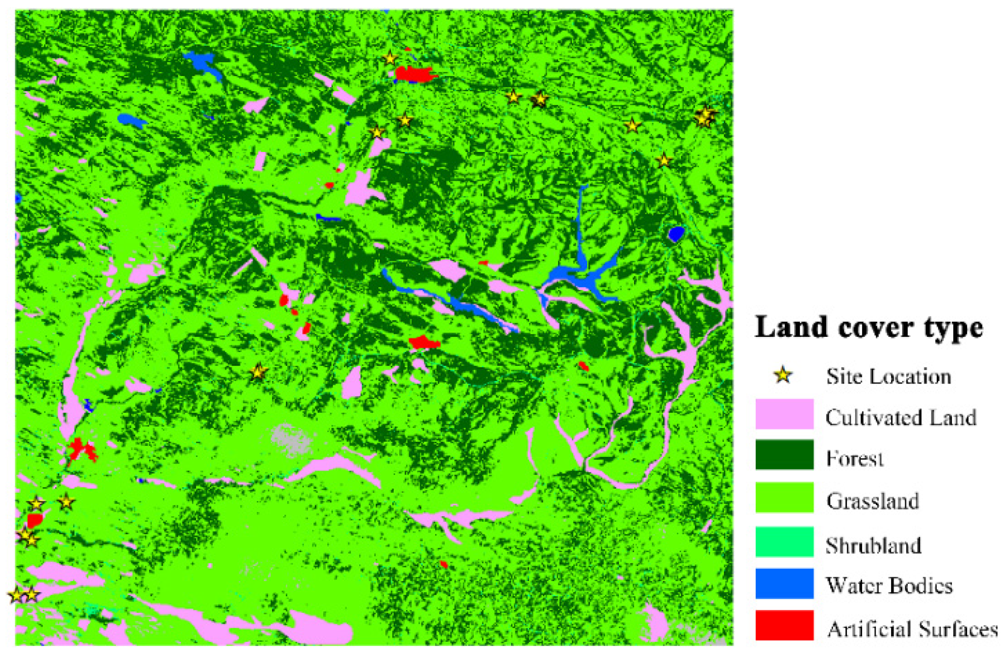
2.1. Study Areas and Field Measurements

Herein, we selected the Saihanba National Park (SNP; Figure 1) for the validation of finer-resolution FVC with field measurements. The SNP area is 666 km2, which is in Hebei Province, China, and consists of 43.2% grassland, 44.0% forest, 9.5% desert and swamp, 3.0% cropland, and 0.3% residential land. The forest is artificial and is dominated by birch and larch. The land cover has a certain heterogeneity but is relatively stable. Field measurements were collected for the primary vegetation types in the SNP.
FVC was measured in sampling plots of 45 m × 45 m by using a digital camera in 2015, to obtain the reference FVC for the validation [21,22,23]. During the experiment, the digital camera was set up at a height of 1.5~2 m from the ground with the help of a long stick, and it was directed downward when photographing. Given the forests in SNP, a top-down direction was used to capture low vegetation underneath the tree crown, whereas a bottom-up direction was used to capture the underside of the tree crown. Additionally, the forest FVC was calculated as Equation (1), in which fup is for tree crown FVC while fdown is for FVC underneath the tree crown. Digital images were taken along two diagonals of the plot, and about 20 images were taken for each plot. The digital FVC images were processed by using an automatic and shadow-resistant algorithm (SHAR-LABFVC) with an uncertainty of less than 0.025 [24]. In all, 25 sites with 35 measurements captured from 27 June to 13 September 2015 were used for evaluation herein (i.e., some sites were measured multiple times during this period).
FVC = f u p + ( 1 f u p ) f d o w n

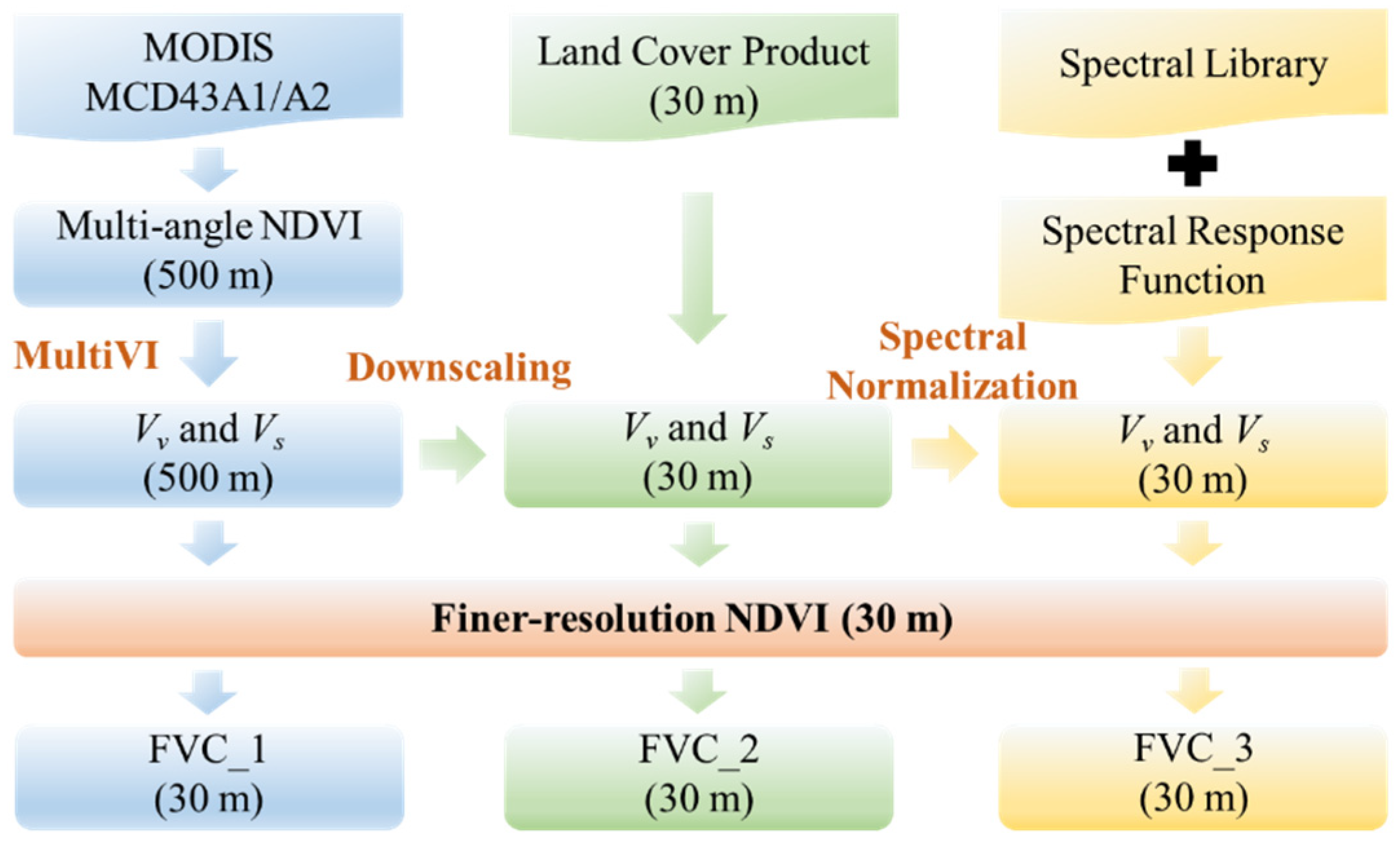
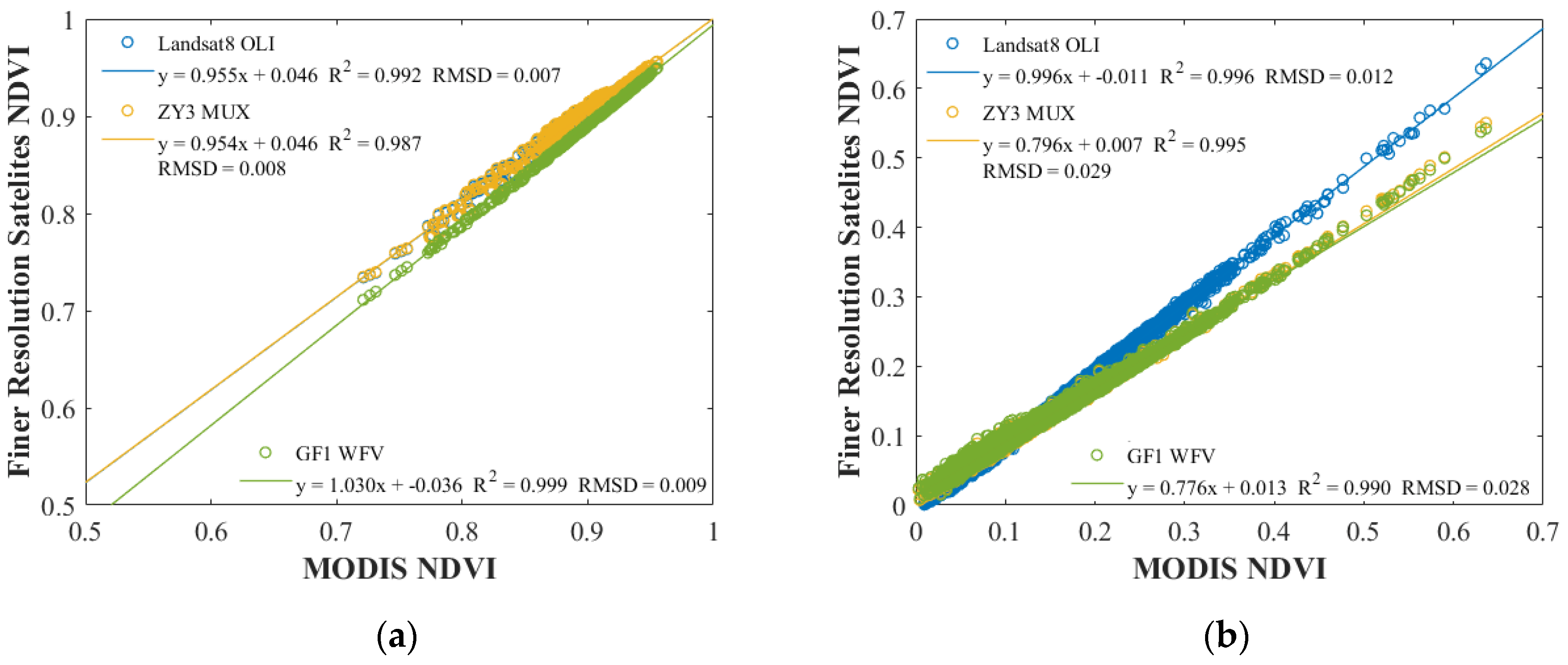
2.2. Finer-Resolution NDVI

To analyze the uncertainty and feasibility of the VI-based mixture model and Vv and Vs from MODIS via MultiVI in finer-resolution FVC estimation, three satellite data were getting involved and compared, being: (i) Landsat 8 OLI surface reflectance product [25]; (ii) Chinese GF 1 satellite wide-field-of-view (WFV; 16 m) data; (iii) Chinese ZY 3 satellite multi-spectral camera (MUX; 5.8 m) data. Table 1 lists the temporal information of these satellite data. An atmospheric correction based on the dark object method was applied to GF 1 data [26]. A 10-day mean temporal composition was applied to GF 1 data to remove outliers. The Fast Line-of-sight Atmospheric Analysis of Hypercubes (FLAASH) module in the Environment for Visualizing Images (ENVI; Exelis, Inc., Boulder, CO, USA) software was used for the atmospheric correction of ZY 3 data. Both GF 1 and ZY 3 surface reflectance were simply averaged aggregated to 30-meter resolution, which was the same as Landsat 8, and NDVI was calculated for FVC estimation.

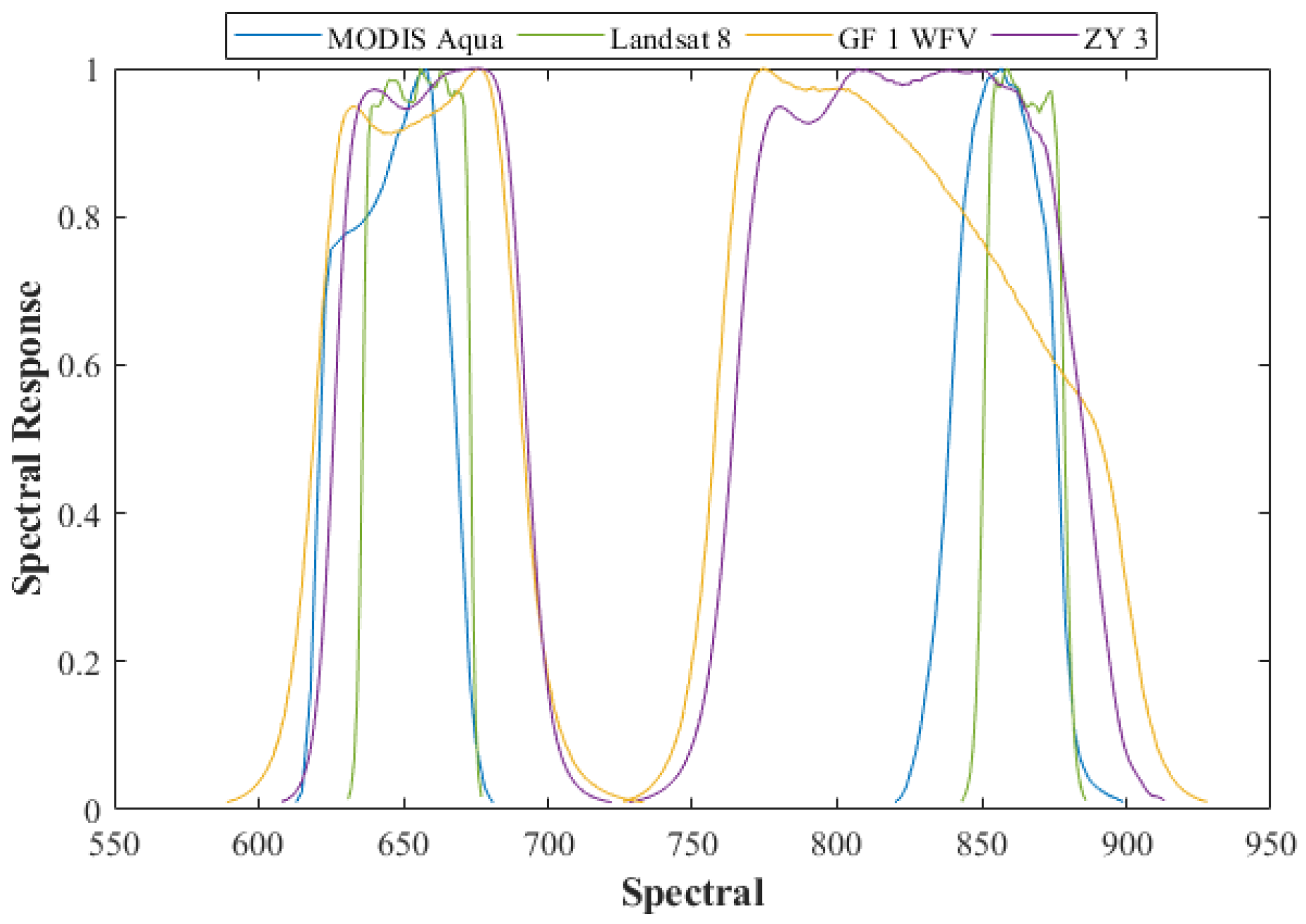
2.3. Spectral Library

The spectral band ranges and spectral response differences among MODIS, Landsat 8, GF 1, and ZY 3 (Figure 2) were analyzed before applying the Vv and Vs from MODIS to the other three finer resolution satellite data. Canopy spectra were simulated based on the three-dimensional (3D) radiative transfer (RT) simulation framework, LESS (large-scale remote sensing data and image simulation framework over heterogeneous 3D scenes) [27]. The RT leaf model, PROSPECT-D [28], built-in LESS was used to simulate different leaves’ spectra. High, middle, and low levels of dry matter (Cm), chlorophyll (Cab), and anthocyanin (Anth) were considered. Table 2 lists the details of the parameters for PROSPECT-D. Canopy structure was defined by Leaf Area Index (LAI), Leaf inclination Angle Distribution (LAD), and crown shape. For canopy spectra simulation, the scene LAI was set at 6, which represented a very dense vegetation scene. The shape of leaf in all scenes was set as disc; details are listed in Table 3. When simulating the canopy spectra, the effects of soil reflectivity were also considered. The soil spectra were from the global spectral libraries [29,30]. In all 486, canopy spectra were simulated and 4439 soil spectra were used for spectral normalization.

2.4. Vv and Vs Downscaling

A 30 m resolution global land cover dataset (GlobeLand 30) in 2010 [31] was used to downscale Vv and Vs from MODIS in 500-meter resolution. GlobeLand 30 divides the land surface into 10 types, including 6 vegetation types (i.e., cultivated land, forest, grassland, shrubland, wetland, and tundra) and 4 unvegetated types (i.e., water bodies, artificial surfaces, bare land, and permanent snow and ice). Herein, we combined the wetland, water bodies, and permanent snow and ice into 1 type, all named water bodies, since they all have Vs below 0. As for MODIS, Vs via MultiVI does not consider the water background and it is always greater than 0; this type was considered in the downscaling process, but no FVC estimation was performed. Thus, 8 land cover types (i.e., cultivated land, forest, grassland, shrubland, tundra, artificial surfaces, bare land, and water bodies) were used for Vv and Vs downscaling.
Vv/Vs for each MODIS pixel is assumed as the combination of Vv/Vs of all land cover types in this pixel area. Take the proportion of each land cover type (k) in the MODIS pixel as the weight (f), 500 m Vv/Vs can be decomposed to 30-meter resolution according to Equation (2).
{ V v , m o d i s = k = 1 m f k V v , k V s , m o d i s = k = 1 m f k V s , k
where, Vv,modis and Vs,modis is the Vv and Vs for a single 500 m MODIS pixel, Vv,k and Vs,k is the Vv and Vs for a single 30 m land cover type (k) pixel, m is the number of land cover type in this MODIS pixel area. A 3 × 3 sliding window with 1 MODIS pixel step was used to solve the equation, and the result was set as the solution for all the 30 m land cover type pixels in the center MODIS pixel area. Equation (3) shows an example of how to obtain Vv,k in MODIS pixel (x,y) using a sliding window. For obtaining Vs,k, it is the same as that of Vv,k, except that Vv,modis is replaced by Vs,modis.
{ V v , m o d i s , x 1 , y 1 = k = 1 m f k , x 1 , y 1 V v , k , x , y V v , m o d i s , x 1 , y = k = 1 m f k , x 1 , y V v , k , x , y V v , m o d i s , x 1 , y + 1 = k = 1 m f k , x 1 , y + 1 V v , k , x , y V v , m o d i s , x , y 1 = k = 1 m f k , x , y 1 V v , k , x , y V v , m o d i s , x , y = k = 1 m f k , x , y V v , k , x , y V v , m o d i s , x , y + 1 = k = 1 m f k , x , y + 1 V v , k , x , y V v , m o d i s , x + 1 , y 1 = k = 1 m f k , x + 1 , y 1 V v , k , x , y V v , m o d i s , x + 1 , y = k = 1 m f k , x + 1 , y V v , k , x , y V v , m o d i s , x + 1 , y + 1 = k = 1 m f k , x + 1 , y + 1 V v , k , x , y

2.5. Spectral Normalization

Spectral normalization was applied to Vv and Vs from MODIS to match spectral settings of Landsat 8, GF 1, and ZY 3. Canopy and soil spectra described in Sec. II.C was transformed into red and near-infrared (NIR) bands reflectance according to the spectral response functions of each satellite sensor (Figure 2). Normalized coefficients for Vv and Vs were obtained based on canopy and soil NDVI, respectively. A simple linear model (Equation (4)) was performed on Landsat 8 and MODIS, GF 1 and MODIS, and ZY 3 and MODIS, respectively.
{ N D V I v e g 1 , i = a v , i · N D V I v e g 1 ,     m o d i s + b v , i N D V I v e g 2 , i = a v , i · N D V I v e g 2 ,     m o d i s + b v , i N D V I v e g j , i = a v , i · N D V I v e g j ,     m o d i s + b v , i N D V I v e g n , i = a v , i · N D V I v e g n ,     m o d i s + b v , i
where, i is for Landsat 8, GF 1, and ZY 3; NDVIvegj,i is the NDVI of i calculated from canopy spectrum j; NDVIvegj,modis is the NDVI of MODIS calculated from canopy spectrum j; av,i and bv,i are normalized coefficients for Vv of i. In all 486 canopy spectra were used for av,i and bv,i estimation; thus, n is 486 in Equation (4). The estimation of the normalized coefficients for Vs of i (i.e., as,i and bs,i) are similar to Vv, except for changing the spectra to the soil. When estimating as,i and bs,i, n was 4439, which means 4439 soil spectra. Vv and Vs for Landsat 8, GF 1, and ZY 3 were calculated by applying the normalized coefficients to Vv and Vs from MODIS.

2.6. FVC Production

VI-based mixture model (Equation (5)) was used to estimate consistent FVC products from multiple satellite data. The central latitude/longitude of each pixel for all satellites were used to match Vv and Vs from MODIS with NDVI from Landsat 8, ZY 3, and GF 1. To analyze the necessity of MODIS Vv and Vs downscaling for finer-resolution FVC estimation, FVC (FVC_1 in Figure 3) was estimated with 500-meter and 30-meter endmembers, respectively. To assess uncertainty due to spectral band ranges and spectral response function differences from different satellite sensors, FVC was also estimated with endmembers before (FVC_2 in Figure 3) and after (FVC_3 in Figure 3) spectral normalization. The necessity of MODIS Vv and Vs downscaling, uncertainty of spectral normalization, and consistency of FVC estimation from different satellites were evaluated by comparing with field-measured FVC.
F V C = N D V I V s V v V s

3. Results

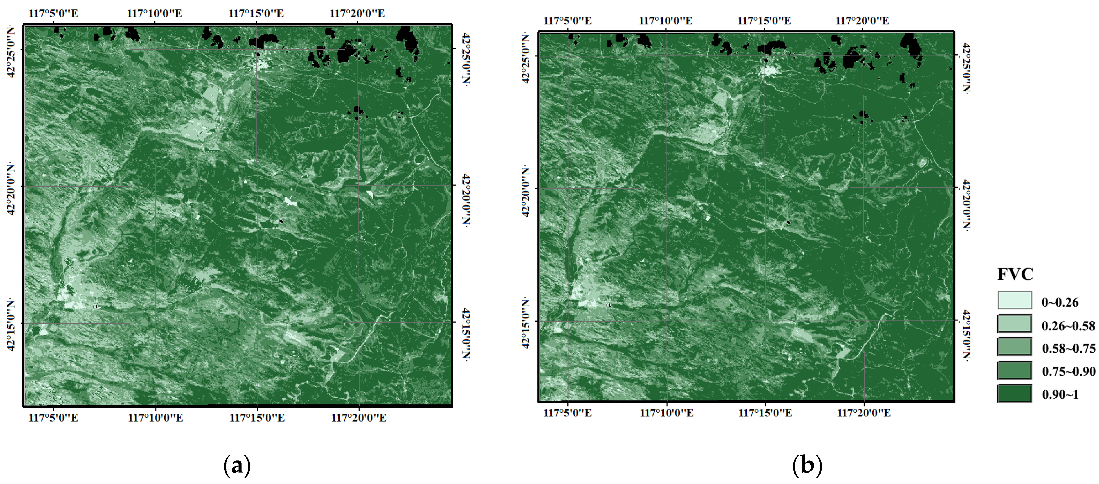
3.1. Necessity Analysis for Vv and Vs Downscaling

The necessity of downscaling the endmembers, Vv and Vs, from MODIS was analyzed by comparing the uncertainty of FVC estimation based on the endmembers at 500 m and 30 m, respectively. Figure 4 shows that FVC from Landsat 8 has lower uncertainty with 30 m Vv and Vs (i.e., RMSD for FVC_2 is 0.124) than with 500 m (i.e., RMSD for FVC_1 is 0.134). However, for ZY 3 and GF 1, the uncertainties are not much different. The RMSDs for FVC_1 and FVC_2 from ZY 3 are 0.117 and 0.119, while for FVC_1 and FVC_2 from GF 1 are 0.094 and 0.102, respectively. The FVC estimation uncertainty of using finer-resolution Vv and Vs depends on the positioning accuracy of the input data (i.e., finer-resolution NDVI). Since the land cover dataset (GlobeLand 30) used for downscaling was produced based on Landsat and HJ satellites [31], the 30 m Vv and Vs have better positioning consistency with FVC from Landsat 8 than ZY 3 and GF 1. As for consistency (R2), FVC_2 for Landsat 8, ZY 3, and GF 1 all have lower consistency than that of FVC_1. The downscaled endmembers increase the heterogeneity of the estimated FVC results. FVC_1 within the same 500-meter resolution pixel only reflects the difference of the 30 m NDVI from Landsat 8, ZY 3, or GF 1. When downscaled endmembers are used, the FVC_2 differences also include differences in land cover types. This shows that the downscaled endmembers have different accuracy under different land cover types, but the overall trend is good (i.e., RMSD decrease).

3.2. Uncertainty Analysis for Spectral Normalization

The uncertainty of FVC estimation caused by the spectral difference between finer-resolution NDVI from Landsat 8, ZY 3, and GF 1 and Vv and Vs from MODIS were analyzed by comparing finer-resolution FVC with field measurement (Table 4). We compared situations of no spectral normalization (i.e., original in Table 4), only normalized Vs, only normalized Vv, and normalized both Vv and Vs (i.e., normalized all in Table 4), respectively. Results show that all Landsat 8, ZY 3, and GF 1 have slight improvement after spectral normalization (i.e., on average, the RMSD of FVC estimated with normalized Vv and Vs decreased ~2.6% compared with the FVC estimated with the original Vv and Vs). Since 30 of the 35 field measurements have FVC > 0.5 (Figure 4), which are more sensitive to Vv during production [32], thus only normalized Vv seems to have the lowest uncertainty for Landsat 8 and ZY 3. That is to say when using the VI-based mixture model to estimate consistent finer-resolution FVC products from Landsat 8, ZY 3, and GF 1, a simple spectral normalization of Vv and Vs can be considered.

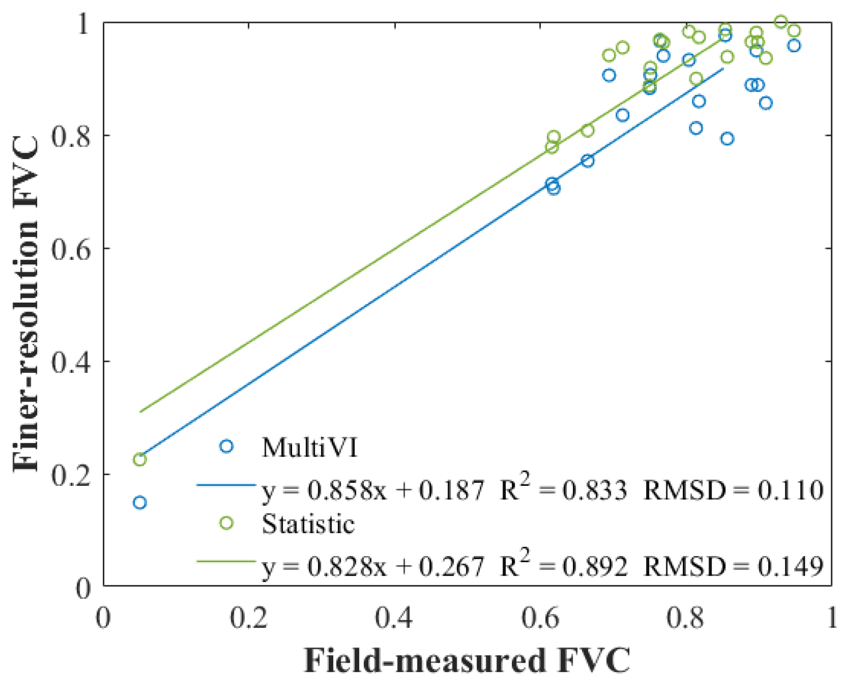
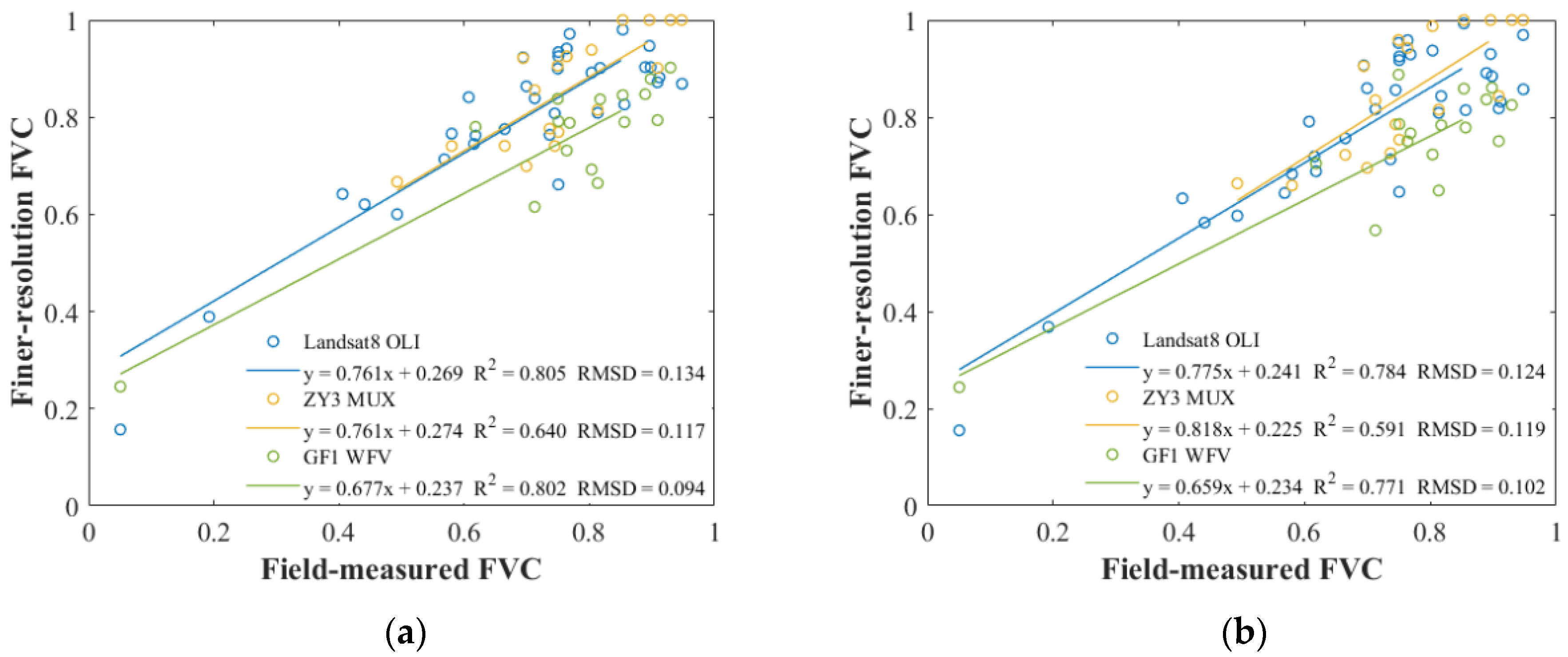
3.3. Accuracy Analysis for FVC by Comparing with Traditional VI-Based Linear Mixture Model

The accuracy of FVC estimated with the process of FVC production in this study was compared with the traditional VI-based linear mixture model. The downscaled MODIS Vv and Vs after spectral normalization were used for the process of FVC production in this study (i.e., FVC_3 was used for comparison). Vv and Vs for the traditional VI-based model were obtained based on the statistic method provided by Zeng et al. [14]. According to Zeng et al. [14], Vv is the NDVI value at the 75th percentile of the cumulative distribution histogram for cultivated land, forest, and grassland, and 90th percentile for shrubland and artificial land, while Vs is the constant value, 0.05, for all land cover types. Considering that Landsat 8 has the highest recognition among all and is the best data match with the GlobeLand 30 land cover product, Landsat 8 on 31 July 2015 was selected for this comparison. Figure 5 shows the FVC map estimated by the proposed method (Figure 5a) and the traditional VI-based linear mixture model (Figure 5b), respectively. The spatial distribution of FVC in both Figure 5a,b is very similar, except that the texture of Figure 5a is clearer. The accuracy of Figure 5a,b was checked by using the field measurements around 31 July 2015. The result (Figure 6) shows that the FVC estimated by the process in this study has less uncertainty (RMSD = 0.110) than the traditional VI-based model (RMSD = 0.149). The lower consistency (R2) is also caused by the heterogeneity of downscaled Vv and Vs.

4. Discussion

4.1. Applicability of the Vv and Vs Downscaling Method

In order to analyze the applicability of the land cover-based Vv and Vs downscaling method used herein, Figure 7 shows the distribution of pixel heterogeneity in the SNP area. The number of different land cover types in each 500-meter MODIS pixel was used to represent the heterogeneity. Herein, most pixels have over two kinds of land cover types but less than six, which makes Equation (3) solvable.
After grouping the field plots based on Figure 7, the uncertainties of estimated FVC from Landsat 8, ZY 3, and GF 1 due to land cover heterogeneity are shown in Figure 8. Here, finer-resolution FVC estimated with downscaled Vv and Vs (FVC_2) was used (Figure 4b). The uncertainty was also presented by absolute error (FVC_2—field-measured FVC). The land cover heterogeneity was grouped into three groups: (1) the number of land cover types is less than three but equal to or greater than two (2 ~ 3); (2) the number of land cover types is less than four but equal or greater than three (3 ~ 4); (3) the number of land cover types is equal or greater than (>4). In Figure 8, the red median marks for both Landsat 8 and ZY 3 FVC are all above the dark red dash zero line in all three groups, which means that they both overestimated the FVC. Due to the small image width of ZY 3, areas with high heterogeneity (>4) are not covered. While for GF 1, both the median and mean are below zero, which means that it underestimated the FVC. The differences in the uncertainty of the estimated FVC hardly change with the heterogeneity (Figure 8), which shows that the surface heterogeneity does not affect the accuracy of the process.
When using a different land cover dataset with a different classification system, the size of the sliding window may need to be adjusted. Furthermore, when it is hard to match finer-resolution Vv, Vs, and finer-resolution NDVI accurately, or land cover product matching the finer-resolution NDVI is not available, particularly in areas that have undergone rapid land cover changes, the coarse-resolution Vv and Vs which represent the average situation of a wide range (herein 500 m × 500 m) and have the closest observation time is better for FVC estimation based on VI-based model. In this study, the positioning accuracy between Landsat 8 and finer-resolution Vv and Vs was less than one pixel, while ZY 3 and GF 1 were worse based on visual interpretation (i.e., within 2~3 pixels).

4.2. Spectral Analysis for Multiple Satellite Sensors

The spectral difference among MODIS, Landsat 8, ZY 3, and GF 1 were compared based on NDVI. Figure 9a shows that the vegetation NDVI (i.e., calculated NDVI based on vegetation spectra described in Sec. II.C) from Landsat 8 and ZY 3 are very similar, while vegetation NDVI from GF 1 looks different. Although ZY 3 has a wide band range, ZY 3 also has a high response in the spectral range, whereas Landsat 8 has a high response, especially in the NIR band (Figure 2); thus, they have very similar vegetation NDVI. As for soil NDVI (i.e., calculated NDVI based on soil spectra described in Sec. II.C), Landsat 8 soil line has the most similarity with MODIS (i.e., has the slope 0.996 very close to 1), while the slopes for ZY 3 and GF 1 are 0.796 and 0.776, respectively (Figure 9b). The influence of the broadband reflectivity of ZY 3 and GF 1 on NDVI is mostly reflected in the soil NDVI.
Different from previous research [19,20], herein, we applied the spectral normalization to Vv and Vs from MODIS to make it match the NDVI from Landsat 8, ZY 3, and GF 1, since Vv and Vs in the VI-based model determine the benchmark and boundary of the FVC estimation [2]. Table 5 lists the original and normalized Vv and Vs. The average Vv for Landsat 8 and ZY 3 are larger than MODIS since the slope of normalized coefficients is less than 1 (Figure 9a). This may be due to the wider high NIR response range of Landsat 8 and ZY 3 than MODIS; the spectral band range (width) with response > 0.9 is 854~875 (21) nm for Landsat 8, 775~871 (96) nm for ZY 3, and 847~864 (17) nm for MODIS (Figure 2). Although GF 1 also has a wide spectral band range, the peak of the NIR spectral response for GF 1 (i.e., 774 nm) is less than others (MODIS: 857 nm, Landsat 8:859 nm, ZY 3: 807 nm; Figure 2). The normalized Vv for GF 1 is less than MODIS. For Vs, all normalized Vs are less than MODIS. There is less difference in the change rate and reflectivity of soil spectra between red and NIR than vegetation. The difference in Vs is mainly caused by the spectral band range.

4.3. Prospect of FVC Estimation by Joint Using Multiple Satellite Data

FVC from finer-resolution satellite data, such as Landsat series, sentinel 2, Chinese GF series, and so on, has great value for dynamic monitoring of crop, city, and hydrological basins [8,9,33]. However, the missed temporal information can hinder applications of FVC that require near-daily or multi-day imagery, flood response, vegetation phenology identification, and forest disturbance detection [8,9,10,33,34]. Only using the temporally sparse time-series satellite data is, therefore, unsuitable for global monitoring of rapid changes and rapid phenology changes. The FVC estimation process proposed in this study can make full use of multiple finer and even high-resolution satellite data. By joint using multiple satellite data for FVC estimation, it is expected to improve the spatial and temporal resolution and applicability of FVC products. The high-frequency and high-spatial-resolution FVC product is meaningful for climate, ecosystem, land degradation, and desertification research [1,2].
In this study, GF 1 (RMSD = 0.099) has the lower uncertainty than Landsat 8 (RMSD = 0.121) and ZY 3 (RMSD = 0.117; Table 4). However, the uncertainty in FVC estimation is influenced not only by the spatial resolution, spectral band range, and spectral response function differences but also by observation geometry. Both Landsat 8 and ZY 3 have nadir view zenith angle (VZA), while GF 1 has a side-swing ability of ≤ 35°, so its VZA changes. Based on a study with the SAIL bidirectional canopy reflectance model coupled with the PROSPECT leaf optical properties model (PROSAIL), the effects of changes in the VZA caused by side sway are found to have a greater impact on reflectance and NDVI than that caused by the spectral response function [19]. Thus, the FVC from GF 1 estimated by the process herein has less stability than FVC from Landsat 8 and ZY 3. For FVC estimation, nadir observation is needed, GF 1 observation with large VZA should be excluded in production.

5. Conclusions

Herein, we provided and analyzed a process of FVC production that is capable of jointly using multiple satellite data. The process is based on the VI-based mixture model with the two key endmembers for pure vegetation (Vv) and bare soil (Vs) from MODIS via the MultiVI method. It is supposed to be able to produce high-frequency and high-temporal FVC products, since multiple finer-resolution satellite data (i.e., Landsat 8, ZY 3, GF 1) can be used to achieve high frequency. The inconsistent spatial resolution between Vv and Vs from MODIS and finer-resolution satellite data and the difference in spectral band range and spectral response function are analyzed. Results shows that FVC from Landsat 8 (RMSD = 0.121), ZY 3 (RMSD = 0.117), and GF 1 (RMSD = 0.099) has uncertainty ~0.11 with downscaled and spectral normalized Vv and Vs. The necessity of Vv and Vs downscaling depends on the positioning accuracy of the finer-resolution satellite data. When the positioning accuracy is worse (i.e., greater than one pixel herein), the coarse-resolution Vv and Vs have less uncertainty during FVC estimation. After spectral normalization, the uncertainty (RMSD) for FVC estimation decreases by ~2.6%.
Therefore, the VI-based mixture model with Vv and Vs from MODIS via MultiVI is flexible in producing FVC at finer resolution and shows potential for the generation of high-frequency large-area products.

Author Contributions

Conceptualization, W.S. and X.M.; methodology, W.S.; software, W.S. and B.Z.; validation, W.S. and T.Z.; formal analysis, L.W.; investigation, T.Z.; resources, B.Z. and J.Z.; data curation, B.Z. and J.Z.; writing—original draft preparation, W.S.; writing—review and editing, W.S., T.Z. and X.M.; visualization, W.S. and T.Z.; supervision, X.M., G.Y., and Z.N.; project administration, G.Y.; funding acquisition, G.Y. and W.S. All authors have read and agreed to the published version of the manuscript.

Funding

This research was funded by the Major Research Plan of the National Natural Science Foundation of China (NSFC; grant number 42090013); and NSFC (grant number 41901273).

Institutional Review Board Statement

Not applicable.

Informed Consent Statement

Not applicable.

Data Availability Statement

Not applicable.

Conflicts of Interest

The authors declare no conflict of interest.

References

  1. Gutman, G.; Ignatov, A. The derivation of the green vegetation fraction from NOAA/AVHRR data for use in numerical weather prediction models. Int. J. Remote Sens. 1998, 19, 1533–1543. [Google Scholar] [CrossRef]
  2. Arneth, A. Climate science: Uncertain future for vegetation cover. Nature 2015, 524, 44–45. [Google Scholar] [CrossRef] [Green Version]
  3. Deardorff, J. Efficient prediction of ground surface temperature and moisture, with inclusion of a layer of vegetation. J. Geophys. Res. Ocean 1978, 83, 1889–1903. [Google Scholar] [CrossRef] [Green Version]
  4. Lu, H.; Raupach, M.R.; McVicar, T.R.; Barrett, D.J. Decomposition of vegetation cover into woody and herbaceous components using AVHRR NDVI time series. Remote Sens. Environ. 2003, 86, 1–18. [Google Scholar] [CrossRef]
  5. Ormsby, J.P.; Choudhury, B.J.; Owe, M. Vegetation spatial variability and its effect on vegetation indices. Int. J. Remote Sens. 1987, 8, 1301–1306. [Google Scholar] [CrossRef]
  6. Carlson, T.N.; Sanchez-Azofeifa, G.A. Satellite Remote Sensing of Land Use Changes in and around San José, Costa Rica. Remote Sens. Environ. 1999, 70, 247–256. [Google Scholar] [CrossRef]
  7. Sellers, P.J.; Tucker, C.J.; Collatz, G.J.; Los, S.O.; Justice, C.O.; Dazlich, D.A.; Randall, D.A. A Revised Land Surface Parameterization (SiB2) for Atmospheric GCMS. Part II: The Generation of Global Fields of Terrestrial Biophysical Parameters from Satellite Data. J. Clim. 1996, 9, 706–737. [Google Scholar] [CrossRef] [Green Version]
  8. Gan, M.; Deng, J.; Zheng, X.; Hong, Y.; Wang, K. Monitoring Urban Greenness Dynamics Using Multiple Endmember Spectral Mixture Analysis. PLoS ONE 2014, 9, e112202. [Google Scholar] [CrossRef]
  9. Pan, J.; Wen, Y. Estimation of soil erosion using RUSLE in Caijiamiao watershed, China. Nat. Hazards 2014, 71, 2187–2205. [Google Scholar] [CrossRef]
  10. Shao, Z.; Cai, J.; Fu, P.; Hu, L.; Liu, T. Deep learning-based fusion of Landsat-8 and Sentinel-2 images for a harmonized surface reflectance product. Remote Sens. Environ. 2019, 235, 111425. [Google Scholar] [CrossRef]
  11. Wang, X.; Jia, K.; Liang, S.; Li, Q.; Wei, X.; Yao, Y.; Zhang, X.; Tu, Y. Estimating Fractional Vegetation Cover From Landsat-7 ETM+ Reflectance Data Based on a Coupled Radiative Transfer and Crop Growth Model. IEEE Trans. Geosci. Remote Sens. 2017, 55, 5539–5546. [Google Scholar] [CrossRef]
  12. Liu, M.; Yang, W.; Chen, J.; Chen, X. An Orthogonal Fisher Transformation-Based Unmixing Method Toward Estimating Fractional Vegetation Cover in Semiarid Areas. IEEE Geosci. Remote Sens. Lett. 2017, 14, 449–453. [Google Scholar] [CrossRef]
  13. Jia, K.; Liang, S.; Gu, X.; Baret, F.; Wei, X.; Wang, X.; Yao, Y.; Yang, L.; Li, Y. Fractional vegetation cover estimation algorithm for Chinese GF-1 wide field view data. Remote Sens. Environ. 2016, 177, 184–191. [Google Scholar] [CrossRef]
  14. Zeng, X.; Dickinson, R.E.; Walker, A.; Shaikh, M.; DeFries, R.S.; Qi, J. Derivation and Evaluation of Global 1-km Fractional Vegetation Cover Data for Land Modeling. J. Appl. Meteorol. 2000, 39, 826–839. [Google Scholar] [CrossRef]
  15. Yang, G.; Pu, R.; Zhang, J.; Zhao, C.; Feng, H.; Wang, J. Remote sensing of seasonal variability of fractional vegetation cover and its object-based spatial pattern analysis over mountain areas. ISPRS J. Photogramm. Remote Sens. 2013, 77, 79–93. [Google Scholar] [CrossRef]
  16. Waldner, F.; Canto, G.S.; Defourny, P. Automated annual cropland mapping using knowledge-based temporal features. ISPRS J. Photogramm. Remote Sens. 2015, 110, 1–13. [Google Scholar] [CrossRef]
  17. Gao, L.; Wang, X.; Johnson, B.A.; Tian, Q.; Wang, Y.; Verrelst, J.; Mu, X.; Gu, X. Remote sensing algorithms for estimation of fractional vegetation cover using pure vegetation index values: A review. ISPRS J. Photogramm. Remote Sens. 2020, 159, 364–377. [Google Scholar] [CrossRef]
  18. Mu, X.; Song, W.; Gao, Z.; McVicar, T.R.; Donohue, R.J.; Yan, G. Fractional vegetation cover estimation by using multi-angle vegetation index. Remote Sens. Environ. 2018, 216, 44–56. [Google Scholar] [CrossRef]
  19. Wang, L.; Yang, R.; Tian, Q.; Yang, Y.; Zhou, Y.; Sun, Y.; Mi, X. Comparative Analysis of GF-1 WFV, ZY-3 MUX, and HJ-1 CCD Sensor Data for Grassland Monitoring Applications. Remote Sens. 2015, 7, 2089. [Google Scholar] [CrossRef] [Green Version]
  20. Li, H.; Chen, Z.-x.; Jiang, Z.-w.; Wu, W.-b.; Ren, J.-q.; Liu, B.; Tuya, H. Comparative analysis of GF-1, HJ-1, and Landsat-8 data for estimating the leaf area index of winter wheat. J. Integr. Agric. 2017, 16, 266–285. [Google Scholar] [CrossRef]
  21. Song, W.; Mu, X.; Ruan, G.; Gao, Z.; Li, L.; Yan, G. Estimating fractional vegetation cover and the vegetation index of bare soil and highly dense vegetation with a physically based method. Int. J. Appl. Earth Obs. Geoinf. 2017, 58, 168–176. [Google Scholar] [CrossRef]
  22. Mu, X.; Huang, S.; Ren, H.; Yan, G.; Song, W.; Ruan, G. Validating GEOV1 fractional vegetation cover derived from coarse-resolution remote sensing images over croplands. IEEE J. Sel. Top. Appl. Earth Obs. Remote Sens. 2015, 8, 439–446. [Google Scholar] [CrossRef]
  23. Mu, X.; Huang, S.; Chen, Y. HiWATER: Dataset of Fractional Vegetation Cover in the middle reaches of the Heihe River Basin. Heihe Plan Sci. Data Cent. 2013. [Google Scholar] [CrossRef]
  24. Song, W.; Mu, X.; Yan, G.; Huang, S. Extracting the Green Fractional Vegetation Cover from Digital Images Using a Shadow-Resistant Algorithm (SHAR-LABFVC). Remote Sens. 2015, 7, 10425. [Google Scholar] [CrossRef] [Green Version]
  25. Vermote, E.; Justice, C.; Claverie, M.; Franch, B. Preliminary analysis of the performance of the Landsat 8/OLI land surface reflectance product. Remote Sens. Environ. 2016, 185, 46–56. [Google Scholar] [CrossRef]
  26. Zhong, B.; Wu, S.; Yang, A.; Liu, Q. An Improved Aerosol Optical Depth Retrieval Algorithm for Moderate to High Spatial Resolution Optical Remotely Sensed Imagery. Remote Sens. 2017, 9, 555. [Google Scholar] [CrossRef] [Green Version]
  27. Qi, J.; Xie, D.; Yin, T.; Yan, G.; Gastellu-Etchegorry, J.-P.; Li, L.; Zhang, W.; Mu, X.; Norford, L.K. LESS: LargE-Scale remote sensing data and image simulation framework over heterogeneous 3D scenes. Remote Sens. Environ. 2019, 221, 695–706. [Google Scholar] [CrossRef]
  28. Féret, J.B.; Gitelson, A.A.; Noble, S.D.; Jacquemoud, S. PROSPECT-D: Towards modeling leaf optical properties through a complete lifecycle. Remote Sens. Environ. 2017, 193, 204–215. [Google Scholar] [CrossRef] [Green Version]
  29. Clark, B.E.; Fanale, F.P.; Salisbury, J.W. Meteorite-asteroid spectral comparison: The effects of comminution, melting, and recrystallization. Icarus 1992, 97, 288–297. [Google Scholar] [CrossRef]
  30. Batjes, N.H. A Globally Distributed Soil Spectral Library Visible Near Infrared Diffuse Reflectance Spectra; World Agroforestry Centre: Nairobi, Kenya, 2014. [Google Scholar]
  31. Chen, J.; Ban, Y.; Li, S. Open access to Earth land-cover map. Nature 2014, 514, 434. [Google Scholar] [CrossRef] [Green Version]
  32. Mu, X.; Zhao, T.; Ruan, G.; Song, J.; Wang, J.; Yan, G.; Mcvicar, T.R.; Yan, K.; Gao, Z.; Liu, Y.; et al. High Spatial Resolution and High Temporal Frequency (30-m/15-day) Fractional Vegetation Cover Estimation over China Using Multiple Remote Sensing Datasets: Method Development and Validation. J. Meteorol. Res. 2021, 35, 128. [Google Scholar] [CrossRef]
  33. Gao, F.; Anderson, M.C.; Zhang, X.; Yang, Z.; Alfieri, J.G.; Kustas, W.P.; Mueller, R.; Johnson, D.M.; Prueger, J.H. Toward mapping crop progress at field scales through fusion of Landsat and MODIS imagery. Remote Sens. Environ. 2017, 188, 9–25. [Google Scholar] [CrossRef] [Green Version]
  34. Yan, G.; Mu, X.; Jia, K.; Song, W.; Liu, Y.; Chen, J.; Gao, Z. Chapter 12—Fractional vegetation cover. In Advanced Remote Sensing, 2nd ed.; Liang, S., Wang, J., Eds.; Academic Press: Cambridge, MA, USA, 2020; pp. 477–510. [Google Scholar] [CrossRef]
Figure 1. Land cover map in the SNP area (50 km × 60 km) from 30 m GlobeLand30 product in 2010. Yellow stars present the 25 site locations.
Forests 13 00691 g001
Figure 2. The spectral response function of MODIS, Landsat 8, GF 1, and ZY 3.
Forests 13 00691 g002
Figure 3. Flowchart of finer-resolution FVC production. Herein, 30 m NDVI was from Landsat 8, GF 1, and ZY 3.
Forests 13 00691 g003
Figure 4. Analysis of FVC estimation using the Vv and Vs of different spatial resolutions. (a) FVC_1: used Vv and Vs at 500 m resolution; (b) FVC_2: used Vv and Vs at 30 m resolution.
Forests 13 00691 g004
Figure 5. FVC map in the SNP area on 31 July 2015. (a) FVC_3 from Landsat 8, which means Vv and Vs are estimated via MultiVI; (b) FVC from Landsat 8 with Vv and Vs from statistic results. The black areas represent no data.
Forests 13 00691 g005
Figure 6. Analysis of FVC estimation in the SNP area on 31 July 2015. The blue line and circles are for FVC_3 from Landsat 8 with Vv and Vs from MultiVI; the green line and circles are for FVC from Landsat 8 with Vv and Vs from statistic results.
Forests 13 00691 g006
Figure 7. The land cover heterogeneity of each 500 m MODIS pixel in the SNP area. The heterogeneity was described by the number of different 30 m land cover types from GlobeLand 30 in 2010.
Forests 13 00691 g007
Figure 8. The error of FVC estimation under different land cover heterogeneity. FVC error is the difference between estimated FVC and field-measured FVC (FVC_2-field-measured FVC). The heterogeneity was described by the number of different 30 m land cover types from GlobeLand 30 in 2010. On each box, the central red mark indicates the median, the number at the top indicates the mean, and the bottom and top edges of the box indicate the 25th and 75th percentiles, respectively. The whiskers extend to the most extreme data points not considered outliers, and the outliers are plotted individually using the red ‘+’ marker symbol. The dark red dash line is the zero line, which means no error. LT 8 is short for Landsat 8.
Forests 13 00691 g008
Figure 9. Spectral normalization between finer-resolution satellite NDVI and MODIS NDVI. (a) is for vegetation; (b) is for soil.
Forests 13 00691 g009
Table 1. The temporal information for satellite data. All data were captured in 2015 which match the field measurements.
DataLandsat 8GF 1ZY 3
Product Time19 June; 5 and 21 July; 6 August; 7 and 23 September30 June; 10 and 30 July; 8 September5 August; 3 September
Table 2. Leaf biochemical parameters for PROSPECT-D. N: structure coefficient; Cm: dry matter; Bp: brown pigments; Car: carotenoids; Cab: chlorophyll; Anth: anthocyanin; Cw: water thickness.
ParametersNCm
(g/cm2)
BpCar
(μg/cm2)
Cab
(μg/cm2)
Anth
(μg/cm2)
Cw
(cm)
Values1.50.005;
0.01;
0.015
01025
50
75
10
20
30
0.025
Table 3. Canopy structure information of the simulated dataset. SZA: solar zenith angle; HOM: homogeneous scene; HET: a heterogeneous scene with spherical crowns; UNI: uniform distribution; SPH: spherical distribution.
SceneObjectObject Radius Object Height LADNumber of Soil TypesSZA
HOMLeaf0.05 m0~15 mUNI;
SPH
30°;
20°;
40°
HETSphere410~19 mUNI;
SPH
30°;
20°;
40°
Table 4. Uncertainty (RMSD) analysis for spectral normalization by comparing finer-resolution FVC (FVC_3) with field measurement. Original: no spectral normalization; Normalized Vs: only did spectral normalization for Vs; Normalized Vv: only did spectral normalization for Vv; Normalized All: did spectral normalization for both Vv and Vs.
SatelliteOriginalNormalized VsNormalized VvNormalized All
Landsat8 OLI0.1240.1260.1190.121
ZY3 MUX0.1190.1220.1140.117
GF1 WFV0.1020.0990.1010.099
Table 5. Vv and Vs statistic over the field sites in SNP in 2015. Vv and Vs for Landsat 8, ZY 3, and GF 1 are the values after spectral normalization. Ave: average; Std.: standard deviation.
Title 1MODISLandsat 8ZY 3GF 1
VvAve.0.8790.8850.8840.869
Std.0.0410.0390.0390.042
VsAve.0.1510.1390.1270.130
Std.0.0320.0320.0250.025
Publisher’s Note: MDPI stays neutral with regard to jurisdictional claims in published maps and institutional affiliations.

