Tractabilities and Intractabilities on Geometric Intersection Graphs ^†

Abstract

A graph is said to be an intersection graph if there is a set of objects such that each vertex corresponds to an object and two vertices are adjacent if and only if the corresponding objects have a nonempty intersection. There are several natural graph classes that have geometric intersection representations. The geometric representations sometimes help to prove tractability/intractability of problems on graph classes. In this paper, we show some results proved by using geometric representations.

1. Introduction

A graph $G=(V,E)$ is said to be an intersection graph if and only if there is a set of objects such that each vertex v in V corresponds to an object $O_v$ and $\{u,v\}\in E$ if and only if $O_v$ and $O_u$ have a nonempty intersection. Interval graphs are a typical intersection graph class, and widely investigated. One reason is that interval graphs have wide applications including scheduling and bioinformatics [1]. Another reason is that an interval graph has a simple structure, and hence we can solve many problems efficiently, whereas the problems are hard in general [1,2]. Some natural generalizations and/or restrictions on interval graphs have been investigated (see, e.g., [2,3,4]). One of the reasons why these intersection graphs are investigated is that their geometric representations sometimes give intuitive simple proof of the tractable/intractable results. On the tractable results, we can solve a problem by using their geometric representations. The geometric representation of a graph gives us an intuitive expression of how to solve a problem using the representation. On the other hand, on the intractable representation, we can express the difficulty of a problem using the geometric representation of a graph. This gives us an intuition of why the problem is difficult to solve. That is, the property of the graph representation also represents the intractableness of the problem. This extracts the essence of the difficulty of the problem and helps us to understand not only the property of the class of graphs, but also the difficulty of the problem.

In this paper, the author reorganizes and shows some related results about graph classes with geometric representations presented at two conferences [5,6] with recent progress. We will mainly consider threshold graphs, chain graphs, and grid intersection graphs. A threshold graph is a graph such that each vertex has a weight, and two vertices are adjacent if and only if their total weight is greater than a given threshold value. The vertex set of a threshold graph is partitioned into two groups such that “light” vertices induce an independent set while “heavy” vertices induce a clique. The threshold graphs form a proper subclass of interval graphs, and can be represented in a compact representation of $O\left(n\right)$ space. A chain graph is a bipartite analogy of the notion of threshold graphs. From a threshold graph, we can obtain a chain graph by removing edges between heavy vertices. In a sense, a chain graph can be seen as a two dimensional extension of a threshold graph. From this viewpoint, a grid intersection graph is a two dimensional extension of an interval graph. More precisely, a bipartite graph $G=(X,Y,E)$ is a grid intersection graph if and only if each vertex $x\in X$ (and $y\in Y$) corresponds to a vertical line (a horizontal line, resp.) such that two vertices are adjacent when they are crossing.

We first focus on a tractable problem on a graph that has a geometric representation. The bandwidth problem is one of the classic problems defined below. A layout of a graph $G=(V,E)$ is a bijection π between the vertices in V and the set $\{1,2,\dots ,\left|V\right|\}$. The bandwidth of a layout π equals $max\{\left|\pi \left(u\right)-\pi \left(v\right)\right|\mid \{u,v\}\in E\}$. The bandwidth of G is the minimum bandwidth of all layouts of G. The bandwidth has been studied since the 1950s; it has applications in sparse matrix computations (see [7,8] for survey). From the graph theoretical point of view, the bandwidth of G is strongly related to the proper interval completion problem [9]. The proper interval completion problem is motivated by research in molecular biology, and hence it attracts much attention (see, e.g., [10]). However, computing the bandwidth of a graph G is one of the basic and classic $\mathcal{NP}$-complete problems [11] (see also [12, GT40]). Especially, it is $\mathcal{NP}$-complete even if G is restricted to a caterpillar with hair length 3 [13]. The bandwidth problem is $\mathcal{NP}$-complete not only for trees, but also for split graphs [14] and convex bipartite graphs [15]. From the viewpoint of exact algorithms, the problem seems to be a difficult one; Feige developed an $O\left({10}^n\right)$ time exact algorithm for the bandwidth problem of general graphs in 2000 [16], and recently, Cygan and Pilipczuk improved it to $O(4.{383}^n)$ time (see [17,18,19] for further details). Therefore approximation algorithms for several graph classes have been developed (see, e.g., [15,20,21,22,23]). Only a few graph classes have been known for which the bandwidth problem can be solved in polynomial time. These include chain graphs [24], cographs and related classes (see [25] for the details), interval graphs [26,27,28], and bipartite permutation graphs [6,29] (see [25] for a comprehensive survey).

One of the interesting graph classes for which the bandwidth problem can be solved efficiently is the class of interval graphs. In 1987, Kratsch proposed a polynomial time algorithm of the bandwidth problem for interval graphs [30]. Unfortunately, the algorithm has a flaw, which has been fixed by Mahesh et al. [27]. Kleitman and Vohra also show a polynomial time algorithm [26], and Sprague improves the time complexity to $O(nlogn)$ by sophisticated implementation of the algorithm [28]. All the algorithms above solve the decision problem that asks if an interval graph G has bandwidth at most k for given G and k. Thus, using binary search for k, we can compute the bandwidth $\mathsf{bw}\left(G\right)$ of an interval graph G in $O\left(M\right(n)·log\mathsf{bw}(G\left)\right)$ time, where $M\left(n\right)=O(nlogn)$ is the time complexity to solve the decision problem [28]. In the literature, it is mentioned that there are two unsolved problems for interval graphs. The first one is direct computation of the bandwidth of an interval graph. All the known algorithms are strongly dependent on the given upper bound k to construct a desired layout. To find a best layout directly, we need deeper insight into the problem and/or the graph class. The second one is to improve the time complexity to linear time. Since interval graphs have a relatively simple representation, many $\mathcal{NP}$-hard problems can be solved in linear time including early results of recognition [31] and graph isomorphism [32].

Another interesting class consists of chain graphs. Chain graphs form a compact subclass of bipartite permutation graphs that plays an important role in developing efficient algorithms for the class of bipartite permutation graphs [33,34]. The algorithm by Kloks, Kratsch, and Müller computes the bandwidth of a chain graph in $O(n^{2}logn)$ time [24]. Their algorithm uses the algorithm for an interval graph as a subroutine, and the factor $O(nlogn)$ comes from the time complexity to solve the bandwidth problem for the interval graph in [28].

In this paper, we propose simple algorithms for the bandwidth problem for the classes of threshold graphs and chain graphs.

The first algorithm computes the bandwidth of a threshold graph G in $O\left(n\right)$ time and space. We note that threshold graphs form a proper subclass of interval graphs, and can be represented in a compact representation of $O\left(n\right)$ space. The algorithm directly constructs an optimal layout, that is, we give a partial answer to the open problem for interval graphs, and improve the previously known upper bound $O(nlognlog\mathsf{bw}(G\left)\right)$ to optimal.

Extending the first algorithm for threshold graphs, we next show an algorithm that computes the bandwidth of a chain graph in $O\left(n\right)$ time and space. This algorithm also directly constructs an optimal layout, and improves the previously known bound $O(n^{2}logn)$ in [24] to optimal.

More precisely, we first give a simple interval representation for a given threshold graph, and simplify the previously known algorithm for interval graphs. (We also show a new property of a previously known algorithm to show correctness.) Next, the simplified interval representation of a threshold graph is extended to the one of a chain graph in a nontrivial way.

Next we turn to the intractable problems on a graph that has a geometric representation. We focus on the class of grid intersection graphs that is a natural bipartite analogy and 2D generalization of the class of interval graphs; a bipartite graph $G=(X,Y,E)$ is a grid intersection graph if and only if G is an intersection graph of X and Y, where X corresponds to a set of horizontal line segments, and Y corresponds to a set of vertical line segments. It is easy to see that the class of chain graphs is a proper subset of the class. Otachi, Okamoto, and Yamazaki investigate relationships between the class of grid intersection graphs and other bipartite graph classes [35]. In this paper, we show that grid intersection graphs have a rich structure. More precisely, we show two hardness results. First, the Hamiltonian cycle problem is still $\mathcal{NP}$-complete even if graphs are restricted to unit length grid intersection graphs. The Hamiltonian cycle problem is one of the classic and basic $\mathcal{NP}$-complete problems [12]. Second, the graph isomorphism problem is still $GI$-complete even if graphs are restricted to grid intersection graphs. (We say the graph isomorphism problem is $GI$-complete if the problem is as hard as to solve the problem on general graphs.) The results imply that (unit length) grid intersection graphs have so rich structure that many other hard problems may still be hard even on (unit length) grid intersection graphs.

We note that they are solvable in linear time on an interval graph [32,36]. Hence we can observe that the generalized interval graphs have so rich structure that some problems become hard on the graphs. Intuitively speaking, the linear (or one dimensional) structure of an interval graph makes these problems tractable, and this two dimensional extension makes them intractable. Such results for intractability also can be found in the literature; the Hamiltonian cycle problem is $\mathcal{NP}$-complete on chordal bipartite graphs [37], and the graph isomorphism problem is $GI$-complete on chordal bipartite graphs and strongly chordal graphs [38].

It is worth mentioning that, recently, the computational complexity of the graph isomorphism problem for circular arc graphs became open again. (A circular arc graph is the intersection graph of circular arcs, which is another natural generalization of an interval graph.) The first “polynomial” time algorithm was given by Wu [39], but Eschen pointed out a flaw [40]. Hsu claimed an $O\left(nm\right)$ time algorithm for the graph isomorphism problem on circular-arc graphs [41]. However, recently, a counterexample to the correctness of the algorithm was found [42].

2. Preliminaries

The neighborhood of a vertex v in a graph $G=(V,E)$ is the set $N_G\left(v\right)=\{u\in V\mid \{u,v\}\in E\}$, and the degree of a vertex v is $\left|N_G\left(v\right)\right|$ denoted by $d_G\left(v\right)$. If no confusion can arise we will omit the index G. For a subset U of V, the subgraph of G induced by U is denoted by $G\left[U\right]$. Given a graph $G=(V,E)$, its complement $\overline{G}=(V,\overline{E})$ is defined by $\overline{E}=\{\{u,v\}\mid \{u,v\}\notin E\}$. A vertex set I is an independent set if and only if $G\left[I\right]$ contains no edges, and then the graph $\overline{G}\left[I\right]$ is said to be a clique. Two vertices u and v are called twins if and only if $N\left(u\right)\cup \left\{u\right\}=N\left(v\right)\cup \left\{v\right\}$.

For a graph $G=(V,E)$, a sequence of distinct vertices $v_0,v_1,\dots ,v_l$ is a path, denoted by $(v_0,v_1,\dots ,v_l)$, if $\{v_j,v_{j+1}\}\in E$ for each $0\le j<l$. The length of a path is the number of edges on the path. For two vertices u and v, the distance of the vertices, denoted by $dist(u,v)$, is the minimum length of the paths joining u and v. A cycle consists of a path $(v_0,v_1,\dots ,v_l)$ of length at least 2 with an edge $\{v_0,v_l\}$, and is denoted by $(v_0,v_1,\dots ,v_l,v_0)$. The length of a cycle is the number of edges on the cycle (equal to the number of vertices). A path P in G is said to be Hamiltonian if P visits every vertex in G exactly once. The Hamiltonian path problem is to determine if a given graph has a Hamiltonian path. The Hamiltonian cycle problem is defined similarly for a cycle. The problems are well known $\mathcal{NP}$-complete problem (see, e.g., [12]).

An edge that joins two vertices of a cycle but is not itself an edge of the cycle is a chord of that cycle. A graph is chordal if every cycle of length at least 4 has a chord. In this paper, we will discuss about intersection graphs of geometrical objects. Interval graphs are characterized by intersection graphs of intervals, and it is well known that chordal graphs are intersection graphs of subtrees of a tree (see, e.g., [2]). A graph $G=(V,E)$ is bipartite if and only if V can be partitioned into two sets X and Y such that every edge joins a vertex in X and the other vertex in Y. We sometimes denote a bipartite graph by $G=(X,Y,E)$ to specify the two vertex sets. A bipartite graph is chordal bipartite if every cycle of length at least 6 has a chord.

A graph $(V,E)$ with $V=\{v_1,v_2,\dots ,v_n\}$ is an interval graph if there is a finite set of intervals $\mathcal{I}=\{I_{v_1},I_{v_2},\dots ,I_{v_n}\}$ on the real line such that $\{v_i,v_j\}\in E$ if and only if $I_{v_i}\cap I_{v_j}\ne \varnothing$ for each i and j with $0<i,j\le n$. We call the set $\mathcal{I}$ of intervals an interval representation of the graph. For each interval I, we denote by $R\left(I\right)$ and $L\left(I\right)$ the right and left endpoints of the interval, respectively (therefore we have $L\left(I\right)\le R\left(I\right)$ and $I=\left[L\right(I),R(I\left)\right]$). An interval representation is called proper if and only if $L\left(I\right)\le L\left(J\right)$ and $R\left(I\right)\le R\left(J\right)$ for every pair of intervals I and J or vice versa. An interval graph is proper if and only if it has a proper interval representation. It is known that the class of proper interval graphs coincides with the class of unit interval graphs [43]. That is, any proper interval graph has a proper interval representation that consists of intervals of unit length (explicit and simple construction is given in [44]). Moreover, each connected proper interval graph has essentially unique proper (or unit) interval representation up to reversal in the following sense (see, e.g., [45]):

Proposition 1 

For any connected proper interval graph $G=(V,E)$ without twins, there is a unique ordering (up to reversal) $v_1,v_2,\dots ,v_n$ of n vertices such that G has a unique proper interval representation $\mathcal{I}\left(G\right)$ such that $L\left(I_{v_1}\right)<L\left(I_{v_2}\right)<\cdots <L\left(I_{v_n}\right)$ (and hence $R\left(I_{v_1}\right)<R\left(I_{v_2}\right)<\cdots <R\left(I_{v_n}\right)$). In other words, for a connected proper interval graph $G=(V,E)$ without twins, there exists a vertex ordering $v_1,v_2,\dots ,v_n$ such that every interval representation of G satisfies either $L\left(I_{v_1}\right)<L\left(I_{v_2}\right)<\cdots <L\left(I_{v_n}\right)$ or $L\left(I_{v_n}\right)<\cdots <L\left(I_{v_2}\right)<L\left(I_{v_1}\right)$.

We note that when G contains twins u and v, they correspond to the congruent intervals with $L\left(I_v\right)=L\left(I_u\right)$ and $R\left(I_v\right)=R\left(I_u\right)$. In a sense, the ordering is still unique even if G contains twins up to isomorphism if the graph is unlabeled.

For any interval representation $\mathcal{I}$ and a point p, $N\left[p\right]$ denotes the set of intervals that contain the point p.

A graph $G=(V,E)$ is called a threshold graph when there exist nonnegative weights $w\left(v\right)$ for all $v\in V$ and a threshold value t such that $\{u,v\}\in E$ if and only if $w\left(u\right)+w\left(v\right)\ge t$.

Let $G=(X,Y,E)$ be a bipartite graph with $X=\{x_1,x_2$, … , $x_n\}$ and $Y=\{y_1,y_2$, … , $y_{n^{\prime }}\}$. The ordering of X has the adjacency property if and only if, for each vertex $y\in Y$, $N\left(y\right)$ consists of vertices that are consecutive in the ordering of X. A bipartite graph $G=(X,Y,E)$ is said to be a chain graph if and only if there are orderings of X and Y that fulfill the adjacency property, and the ordering of X satisfies that $N\left(x_n\right)\subseteq N\left(x_{n-1}\right)\subseteq \cdots \subseteq N\left(x_1\right)$. (The last property implies that the ordering of Y also satisfy $N\left(y_1\right)\subseteq N\left(y_2\right)\subseteq \cdots \subseteq N\left(y_{n^{\prime }}\right)$; see, e.g., [46].)

A graph $G=(V,E)$ with $V=\{v_1,v_2,\dots ,v_n\}$ is said to be a permutation graph if and only if there is a permutation σ over V such that $\{v_i,v_j\}\in E$ if and only if $(i-j)(\sigma \left(v_i\right)-\sigma \left(v_j\right))<0$. Intuitively, each vertex v in a permutation graph corresponds to a line segment ${\ell }_v$ joining two points on two parallel line segments $L_1$ and $L_2$. Then two vertices v and u are adjacent if and only if the corresponding line segments ${\ell }_v$ and ${\ell }_u$ intersect. The ordering of vertices gives the ordering of the points on $L_1$, and the permutation of the ordering gives the ordering of the points on $L_2$. We call the intersection model a line representation of the permutation graph. When a permutation graph is bipartite, it is said to be a bipartite permutation graph. Although a permutation graph has (exponentially) many line representations, a connected bipartite graph essentially has a unique line representation up to isomorphism (see [47] for further details):

Lemma 2 

Let $G=(V,E)$ be a connected bipartite permutation graph without twins. Then the line representation of G is unique up to isomorphism.

The following proper inclusions are known (see, e.g., [46,48]):

Lemma 3 

(1) Threshold graphs ⊂ interval graphs; (2) chain graphs ⊂ bipartite permutation graphs.

A natural bipartite analogy of interval graphs are called interval bigraphs which are intersection graphs of two-colored intervals so that we do not join two vertices if they have the same color. Based on the definition, Müller showed that the recognition problem for interval bigraphs can be solved in polynomial time [49]. Later, Hell and Huang show an interesting characterization of interval bigraphs, which is based on the idea to characterize the complements of the graphs [50]. Recently, efficient recognition algorithm based on forbidden graph patterns is developed by Rafiey [51].

A bipartite graph $G=(X,Y,E)$ is a grid intersection graph if every vertex $x\in X$ and $y\in Y$ can be assigned line segments $I_x$ and $J_y$ in the plane, parallel to the horizontal and vertical axis so that for all $x\in X$ and $y\in Y$, $\{x,y\}\in E$ if and only if $I_x$ and $J_y$ cross each other. We call $(\mathcal{I},\mathcal{J})$ a grid representation of G, where $\mathcal{I}=\{I_x\mid x\in X\}$ and $\mathcal{J}=\{J_y\mid y\in Y\}$. A grid representation is unit if all line segments in the representation have the same (unit) length. A bipartite graph is a unit grid intersection graph if it has a unit grid representation.

Otachi, Okamoto, and Yamazaki show some relationship between (unit) grid intersection graphs and other graph classes [35]; for example, interval bigraph is included in the intersection of unit grid intersection graphs and chordal bipartite graphs. It is worth mentioning that it is open whether chordal bipartite graphs are included in grid intersection graphs or not.

Two graphs $G=(V,E)$ and $G^{\prime }=(V^{\prime },E^{\prime })$ are isomorphic if and only if there is a one-to-one mapping $\varphi :V\to V^{\prime }$ such that $\{u,v\}\in E$ if and only if $\{\varphi \left(u\right),\varphi \left(v\right)\}\in E^{\prime }$ for every pair of vertices $u,v\in V$. We denote by $G\sim G^{\prime }$ if G and $G^{\prime }$ are isomorphic. The graph isomorphism (GI) problem is to determine if $G\sim G^{\prime }$ for given graphs G and $G^{\prime }$. A graph class $\mathcal{C}$ is said to be $GI$-complete if there is a polynomial time reduction from the graph isomorphism problem for general graphs to the graph isomorphism problem for $\mathcal{C}$. Intuitively, the graph isomorphism problem for the class $\mathcal{C}$ is as hard as the problem for general graphs if $\mathcal{C}$ is $GI$-complete. The graph isomorphism problem is $GI$-complete for several graph classes; for example, chordal bipartite graphs, and strongly chordal graphs [38]. On the other hand, the graph isomorphism problem can be solved efficiently for many graph classes; for example, interval graphs [32], probe interval graphs [52], permutation graphs [53], directed path graphs [54], and distance hereditary graphs [55].

3. Polynomial Time Algorithms for the Bandwidth Problem

A layout of a graph $G=(V,E)$ on n vertices is a bijection π between the vertices in V and the set $\{1,2,\dots ,n\}$. The bandwidth of a layout π equals $max\{\left|\pi \left(u\right)-\pi \left(v\right)\right|\mid \{u,v\}\in E\}$. The bandwidth of G, denoted by $\mathsf{bw}\left(G\right)$, is the minimum bandwidth of all layouts of G. A layout achieving $\mathsf{bw}\left(G\right)$ is called an optimal layout. On a layout π, we denote by $S<S^{\prime }$ for two vertex sets $S,S^{\prime }$ if and only if $\pi \left(u\right)<\pi \left(v\right)$ holds for every pair of $u\in S$ and $v\in S^{\prime }$.

For given graph $G=(V,E)$, a proper interval completion of G is a superset $E^{\prime }$ of E such that $G^{\prime }=(V,E^{\prime })$ is a proper interval graph. Hereafter, we will omit the “proper interval” since we always consider proper interval completions. We say a completion $E^{\prime }$ is minimum if and only if $\left|C^{\prime }\right|\le \left|C^{″}\right|$ for maximum cliques $C^{\prime }$ in $G^{\prime }=(V,E^{\prime })$ and $C^{\prime \prime }$ in $G^{\prime \prime }=(V,E^{″})$ for any other completion $E^{\prime \prime }$.

For a minimum completion $E^{\prime }$, it is known that $\mathsf{bw}\left(G\right)=\left|C^{\prime }\right|-1$, where $C^{\prime }$ is a maximum clique in $G^{\prime }=(V,E^{\prime })$ [9]. Let $G=(V,E)$ be an interval graph with an interval representation $\mathcal{I}=\{I_{v_1},I_{v_2},\dots ,I_{v_n}\}$. For each maximal clique C, there is a point p such that $N\left[p\right]$ induces the clique C by Helly property. Thus, for any given graph G, we can compute $\mathsf{bw}\left(G\right)$ by Algorithm 1.

Algorithm 1: Bandwidth of a general graph

Input : Graph G = (V,E)

Output: $\mathsf{bw}\left(G\right)$  generate a proper interval graph $G^{\prime }=(V,E^{\prime })$ that gives a minimum completion of G  make the unique proper interval representation $\mathcal{I}\left(G^{\prime }\right)$ of $G^{\prime }$  find a point p such that $\left|N\left[p\right]\right|\ge \left|N\left[p^{\prime }\right]\right|$ for any other point $p^{\prime }$ on $\mathcal{I}\left(G^{\prime }\right)$

returen ($\left|N\left[p\right]\right|-1$).

In Algorithm 1, the key point is how to find the minimum completion of G in the first step. The following observation may not be explicitly given in literature, but it can be obtained from the results in [9] straightforwardly (for example, the proof of Theorem 3.2 in [9], this fact is implicitly used):

Observation 4 

For a minimum completion $G^{\prime }=(V,E^{\prime })$ of $G=(V,E)$, let $\mathcal{I}\left(G^{\prime }\right)=(I_{v_1}^{\prime },I_{v_2}^{\prime },\dots ,I_{v_n}^{\prime })$ be the unique proper interval representation of $G^{\prime }$ stated in Proposition 1. Then the ordering $v_1,v_2,\dots ,v_n$ gives an optimal layout of G, and vice versa.

Here we show a technical lemma for the proper interval subgraph of an interval graph that will play an important role of our results.

Lemma 5 

Let $G=(V,E)$ be an interval graph with $V=\{v_1,v_2,\dots ,v_n\}$, and $\mathcal{I}=\{I_{v_1},I_{v_2},\dots ,I_{v_n}\}$ an interval representation of G. Let $\mathcal{J}=\{J_{u_1},J_{u_2},\dots ,J_{u_k}\}$ be a subset of $\mathcal{I}$ such that $\mathcal{J}$ forms a proper interval representation. That is, we have $U=\{u_1,\dots ,u_k\}\subseteq V$, and we can order $\mathcal{J}$ as $L\left(J_{u_i}\right)\le L\left(J_{u_{i+1}}\right)$ and $R\left(J_{u_i}\right)\le R\left(J_{u_{i+1}}\right)$ for each $1\le i<k$. Let ρ be the injection from $\mathcal{J}$ to $\mathcal{I}$ with $J_{u_i}=I_{v_{\rho \left(i\right)}}$ for each $1\le i\le k\le n$. Then, G has an optimal layout π such that each interval $J_{u_i}$ appears according to the ordering in $\mathcal{J}$. More precisely, for each i with $1\le i<k$, we have $\pi \left(v_{\rho \left(i\right)}\right)<\pi \left(v_{\rho (i+1)}\right)$.

Proof. The proof is strongly related to the algorithm, which we call Algorithm KV, developed by Kleitman and Vohra in [26]. To be self-contained, we give a description of Algorithm KV in Appendix A. We recall that for given an interval representation of an interval graph $G=(V,E)$ and a positive integer k, Algorithm KV constructs a layout π of V that achieves the bandwidth at most k if $\mathsf{bw}\left(G\right)\le k$. The main idea is as follows. We assume that we give the interval representation $\mathcal{I}$ and $\mathsf{bw}\left(G\right)$ as an input to Algorithm KV. Through the construction of the optimal layout π, indeed, Algorithm KV does not change the ordering in $\mathcal{J}$. We note that Algorithm KV itself does not mind the set $\mathcal{J}$. That is, for an interval graph $G=(V,E)$, Algorithm KV does not change the ordering of any subset $\mathcal{J}$ if $\mathcal{J}$ induces a proper interval graph.

Basically, Algorithm KV greedily labels each interval from 1 to n, from left to right. Unlabeled intervals are divided into two groups; the intervals incident to labeled intervals and others. The former group is again divided into sets $S_j^q$. A set $S_j^q$ contains unlabeled intervals that should have labels up to $(j+q)$, where q is the largest label so far. In the first saturated $S_j^q$ with respect to $(j+q)$, the interval having the smallest left endpoint is chosen as the next interval (ties are broken by the right endpoints).

To prove the lemma, we have to show the leftmost unlabeled interval $J_{u_i}$ in $\mathcal{J}$ has to be chosen before $J_{u_{i+1}}$ when Algorithm KV chooses an interval in $\mathcal{J}$. When Algorithm KV picks up the first saturated $S_j^q$ in Step 7, we have $S_1^q\subseteq S_2^q\subseteq \cdots \subseteq S_j^q$. Hence, by a simple property of proper intervals, $S_j^q$ contains all unlabeled $J_{u_i}$ with $i^{\prime }<i\le i^{\prime \prime }$ such that $J_{u_{i^{\prime }}}$ is the rightmost labeled interval in $\mathcal{J}$ and $J_{u_{i^{″}}}$ is the rightmost unlabeled interval in $\mathcal{J}$ that is adjacent to a labeled interval. Among them, Algorithm KV picks up the interval that has the smallest left endpoint (in Step 2 or 8). Thus, with appropriate tie-breaking, the next labeled interval can be $J_{u_{i^{\prime }+1}}$ before $J_{u_{i^{\prime }+2}}$. Therefore, Algorithm KV labels all intervals in $\mathcal{J}$ from left to right, and we have the lemma.      ■

3.1. Linear Time Algorithm for a Threshold Graph

We first show a linear time algorithm for computing $\mathsf{bw}\left(G\right)$ of a connected threshold graph G. For a threshold graph $G=(V,E)$, there exist nonnegative weights $w\left(v\right)$ for $v\in V$ and t such that $\{u,v\}\in E$ if and only if $w\left(u\right)+w\left(v\right)\ge t$. We assume that a threshold graph is given in the standard adjacency list manner. That is, each vertex has its own neighbor list and it knows its degree and weight. We assume that G is connected and V is already ordered as $\{v_1,v_2,\dots ,v_n\}$ with $w\left(v_i\right)\le w\left(v_{i+1}\right)$ for $1\le i<n$ (this sort can be done in $O\left(n\right)$ time by a standard bucket sort [56, Section 5.2.5] according to the degrees of vertices; ties may occur by twins, and are broken in any way). We can find ℓ such that $w\left(v_{\ell -1}\right)+w\left(v_{\ell }\right)<t$ and $w\left(v_{\ell }\right)+w\left(v_{\ell +1}\right)\ge t$ in $O\left(n\right)$ time. Then G has the following interval representation $\mathcal{I}\left(G\right)$:

• For $1\le i\le \ell$, $v_i$ corresponds to the point i, that is, $I_{v_i}=[i,i]$.
• For $\ell <i\le n$, $v_i$ corresponds to the interval $[j,\ell ]$, where j is the minimum index with $w\left(v_i\right)+w\left(v_j\right)\ge t$.

For example, Figure 1(a) is a threshold graph; each number in a circle is its weight, and threshold value is 5. We have $\ell =5$ and its interval representation is given in Figure 1(b).

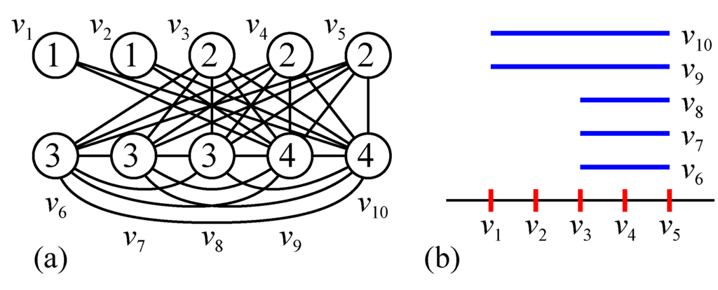
Figure 1. (a) Threshold graph and (b) its interval representation.

Figure 1. (a) Threshold graph and (b) its interval representation.

Theorem  6 

We assume that a connected threshold graph $G=(V,E)$ is given in the interval representation $\mathcal{I}\left(G\right)$ stated above. Then we can compute $\mathsf{bw}\left(G\right)$ in $O\left(n\right)$ time and space.

Proof. We first observe that $L\left(I_{v_i}\right)<L\left(I_{v_{i+1}}\right)$ and $R\left(I_{v_i}\right)<R\left(I_{v_{i+1}}\right)$ for each $v_i$ with $1\le i<\ell$, and $L\left(I_{v_i}\right)\ge L\left(I_{v_{i+1}}\right)$ and $R\left(I_{v_i}\right)=R\left(I_{v_{i+1}}\right)=\ell$ for each i with $\ell <i<n$. That is, G consists of two proper interval graphs induced by $\{v_1,v_2,\dots ,v_{\ell }\}$ and $\{v_{\ell },v_{\ell +1},\dots ,v_n\}$ (note that $v_{\ell }$ is shared). Their proper interval representations also appear in $\mathcal{I}\left(G\right)$. Hence, by Lemma 5, there exists an optimal layout π of $V=\{v_1,\dots ,v_n\}$ such that $\pi \left(v_1\right)<\pi \left(v_2\right)<\cdots <\pi \left(v_{\ell }\right)$ and $\pi \left(v_{\ell }\right)>\pi \left(v_{\ell +1}\right)>\pi \left(v_{\ell +2}\right)>\cdots >\pi \left(v_n\right)$. Thus we can obtain an optimal layout by merging two sequences of vertices.

To obtain an optimal layout, by Observation 4, we construct a minimum completion of G from two sequences. The longest interval is given by $v_n$; since G is connected, $[L\left(I_{v_n}\right),R\left(I_{v_n}\right)]=[1,\ell ]$. Hence, we extend all intervals (except $I_{v_n}$) to length $\ell -1$ and construct a minimum completion. We denote the extended interval $I_{v_i}$ by $I_{v_i}^{\prime }$. That is, the length of $I_{v_i}^{\prime }=\ell -1$ for all i with $1\le i\le n$. The extension is illustrated in Figure 2. The extension of intervals $I_{v_i}$ for $i>\ell$ is straightforward; just extend them to the right, which does not increase the size of a maximum clique. Thus we focus on the points $I_{v_i}=[i,i]$ with $i\le \ell$, which are extended to $I_{v_i}^{\prime }$ with length $\ell -1$.

Figure 2. Construction of a minimum completion.

Figure 2. Construction of a minimum completion.

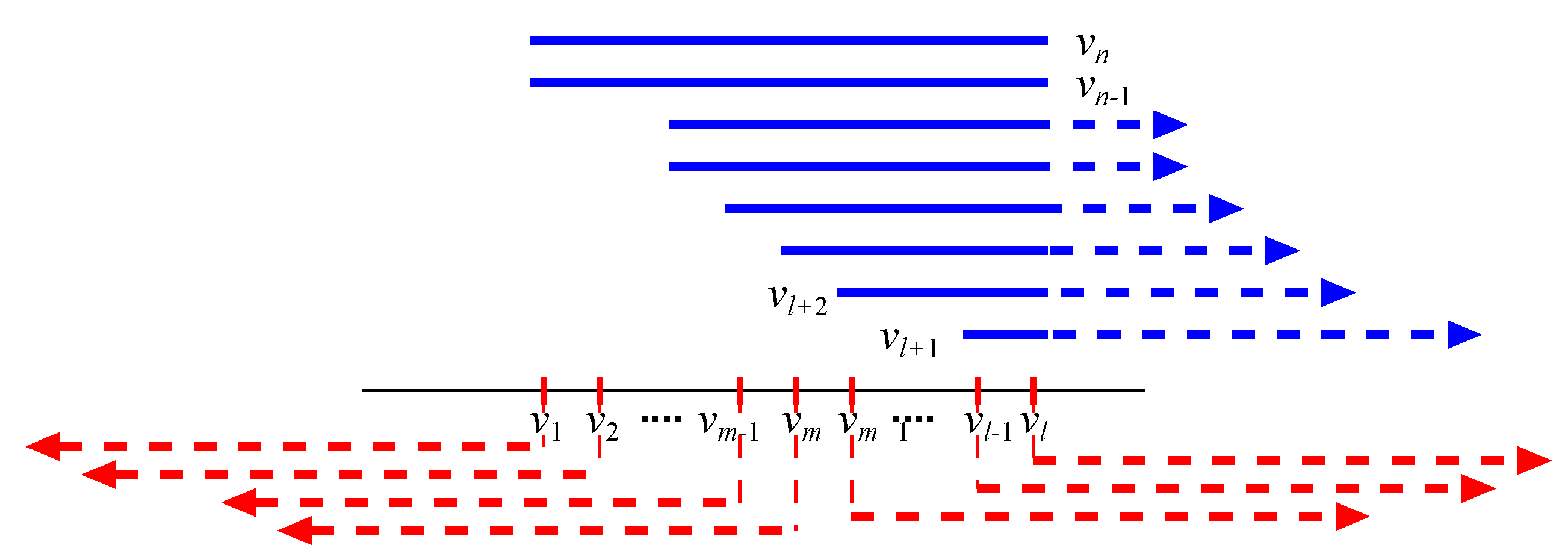
If $I_{v_i}^{\prime }$ does not contain the point 1, $I_{v_i}^{\prime }$ has to contain the point ℓ since it has to have length $\ell -1$. On the other hand, once $I_{v_i}^{\prime }$ contains the point ℓ, we can set $I_{v_i}^{\prime }=[i..\ell +i-1]$ without loss of generality. Otherwise, the size of a maximum clique at the left side of the point i may increase. Similarly, once $I_{v_i}^{\prime }$ does not contain the point ℓ, we can set $I_{v_i}^{\prime }=[-\ell +i+1..i]$ without loss of generality. That is, we can assume that $L\left(I_{v_i}^{\prime }\right)=i$ or $R\left(I_{v_i}^{\prime }\right)=i$ for each $1\le i\le \ell$. If two intervals $I_{v_i}^{\prime }$ and $I_{v_j}^{\prime }$ satisfy $i<j\le \ell$, $L\left(I_{v_i}^{\prime }\right)=i$, and $R\left(I_{v_j}^{\prime }\right)=j$, we can make $R\left(I_{v_i}^{\prime }\right)=i$, and $L\left(I_{v_j}^{\prime }\right)=j$ without increasing the size of a maximum clique. Specifically, we can take $R\left(I_{v_1}^{\prime }\right)=1$ and $L\left(I_{v_{\ell }}^{\prime }\right)=\ell$.

From the above observation, a minimum completion is given by the following proper interval representation of n intervals of length $\ell -1$ for some m with $1\le m<\ell$: (0) for each $i>\ell$, $L\left[I_{v_i}\right]=j$, where j is the minimum index with $w\left(v_i\right)+w\left(v_j\right)\ge t$; (1) for each $1\le i\le m$, $R\left[I_{v_i}\right]=i$, and (2) for each $m<i\le \ell$, $L\left[I_{v_i}\right]=i$ (Figure 2). Thus, to construct a minimum completion, we search the index m that minimizes a maximum clique in the proper interval graph represented by above proper interval representation determined by m.

In the minimum completion, there are ℓ distinct cliques $C_i=N\left[i\right]$, one induced at each point i with $1\le i\le \ell$. Now we consider a maximum clique of the corresponding proper interval graph for a fixed $m\in [1..\ell ]$.

At points in $[m+1..\ell ]$, it is easy to see that $N[m+1]\subseteq \cdots \subseteq N\left[\ell \right]$ and hence the point ℓ induces maximum clique of size $(n-(\ell +1)+1)+(\ell -(m+1)+1)=(n-m)$.

We next consider each point i in $[1..m]$. At the point i, $N\left[i\right]$ induces a clique that consists of $\{v_i,v_{i+1},\dots ,v_m\}$ and $\{v_j,v_{j+1},\dots ,v_n\}$, where j is the minimum index with $w\left(v_i\right)+w\left(v_j\right)\ge t$. Hence we have a clique of size $(m-i+1)+(n-j+1)$ at point i. Thus we have to find i in $[1..m]$ that gives a maximum one.

Therefore, for a fixed m, we compute these two candidates for a maximum clique from $[1..m]$ and $[m+1..\ell ]$, compare them, and obtain a maximum one. For every m, we have to find a minimum one of the maximum cliques, whose size gives $\mathsf{bw}\left(G\right)+1$. Thus we can compute $\mathsf{bw}\left(G\right)$ by Algorithm 2.

Algorithm 2: Bandwidth of a threshold graph

Input : Threshold graph G = (V, E) with w(v1 ≤ w(v2) ≤ … ≤ w(vn) and t  Output: $\mathsf{bw}\left(G\right)$  let ℓ be the minimum index with 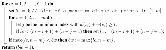$w\left(v_{\ell }\right)+w\left(v_{\ell +1}\right)\ge t$  set $bw:=\infty$

The correctness of Algorithm 2 follows from Observation 4, Lemma 5 and the above discussions.

Algorithm 2 runs in $O\left(n^2\right)$ time and $O\left(n\right)$ space by a straightforward implementation. However, careful implementation achieves $O\left(n\right)$ time and space as follows. When the algorithm updates m in step 3, the proper interval representation does not change except for one vertex $v_{m+1}$. We assume that the value of the variable m is changed from $m^{\prime }$ to $m^{″}=m^{\prime }+1$. Then, the interval $I_{v_{m^{\prime \prime }}}^{\prime }$ is “flipped” from right to left centered at $m^{\prime \prime }$. More precisely, changing from $m^{\prime }$ to $m^{″}=m^{\prime }+1$ means changing $I_{v_{m^{\prime \prime }}}^{\prime }$ from $[m^{″}..\ell +m^{″}-1]$ to $[-\ell +m^{″}+1..m^{″}]$, or equivalently, from $L\left(I_{v_{m^{\prime \prime }}}^{\prime }\right)=m^{″}$ to $R\left(I_{v_{m^{\prime \prime }}}^{\prime }\right)=m^{″}$. This flip has two influences: First, the variable $lc$, which was the size of a maximum clique in $[1..m^{\prime }]$, will be updated by either (1) current $lc+1$ (added by $v_{m^{″}}$ since it is flipped from $L\left(I_{v_{m^{\prime \prime }}}\right)=m^{″}$ to $R\left(I_{v_{m^{\prime \prime }}}\right)=m^{″}$) or (2) $n-j+2$, which is the size of clique induced at the new point $m^{\prime \prime }$, where j is the minimum index with $w\left(v_{m^{\prime \prime }}\right)+w\left(v_j\right)\ge t$. Second, the maximum clique in the range $[m^{″}+1..\ell ]$ is updated from $(n-m^{\prime })$ to $(n-m^{″})$. Thus, to find a maximum clique in the range $[1..m^{″}]$, the algorithm does not need to check all indices in $[1..m^{″}]$ by the for-loop in steps 5 to 8. Precisely, we move step 4 to between steps 2 and 3, and replace the for-loop in steps from 5 to 8 by the following steps;

• let j be the minimum index with $w\left(v_m\right)+w\left(v_j\right)\ge t$;
• set $lc:=max\{lc+1,n-j+2\}$;

We can precompute a table that gives the minimum index j with $w\left(v_i\right)+w\left(v_j\right)\ge t$ for each i in $O\left(n\right)$ time. Using the table, the modified algorithm runs in $O\left(n\right)$ time and space.      ■

We assume that a connected threshold graph $G=(V,E)$ is given in the interval representation $\mathcal{I}\left(G\right)$ stated above. Let $V_0$ and $V_1$ be the sets of light and heavy vertices $v_i$ with $i\le \ell$ and $i>\ell$, respectively. Then, for a connected threshold graph $G=(V,E)$, we have an optimal layout that satisfies $V_0^0<V_1<V_0^1$, where $V_0^0$ and $V_0^1$ are a partition of $V_0$ such that $w\left(v\right)<w\left(u\right)$ for each $v\in V_0^0$ and $u\in V_0^1$. Moreover, the optimal layout gives a maximum clique $G^{\prime }[V_1\cup V_0^1]$ of the graph $G^{\prime }=(V,E^{\prime })$ where $E^{\prime }$ is the completion. We can also partition $V_1$ into $V_1^0=\{v_n,v_{n-1},\dots ,v_{m^{\prime }}\}$ and $V_1^1=\{v_{m^{\prime }-1},\dots ,v_{\ell +1}\}$ such that $N\left(v_m\right)=\{v_n,\dots ,v_{m^{\prime }}\}$ on $G=(V,E)$. Then we can observe that any arrangement of vertices in $V_0^1\cup V_1^1$ gives us an optimal layout. The following corollary will give us an important property in a chain graph.

Corollary 7 

For a connected threshold graph $G=(V,E)$, we have an optimal layout with indices m and $m^{\prime }$ such that $V_0^0<V_1^0<(V_0^1\cup V_1^1)$ and any arrangement of vertices in $V_0^1\cup V_1^1$ gives an optimal layout. Moreover, there is no edge between $u\in V_0^0$ and $v\in V_0^1\cup V_1^1$ on the completion.

3.2. Linear Time Algorithm for a Chain Graph

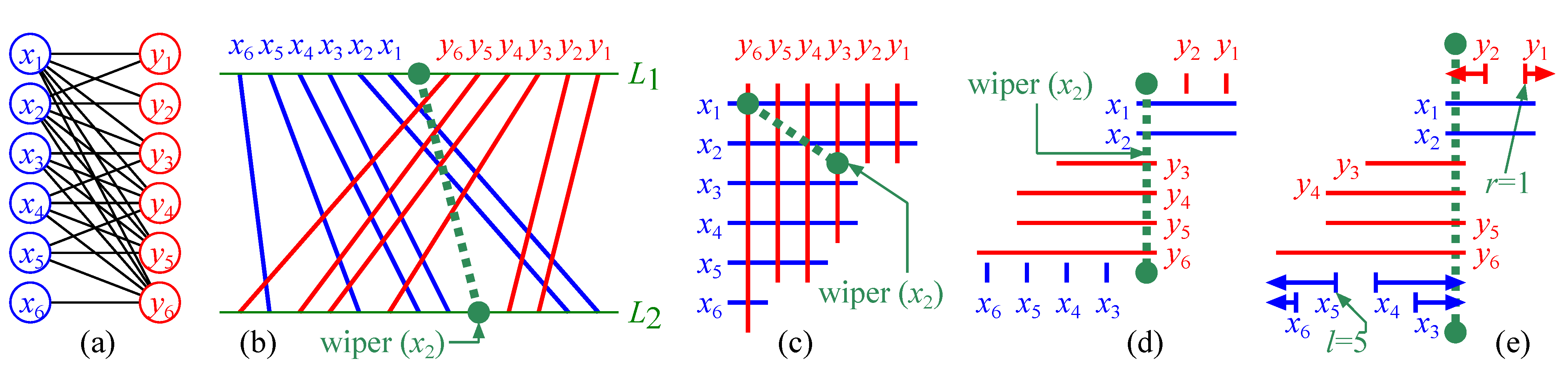
We next show a linear time algorithm for computing $\mathsf{bw}\left(G\right)$ of a connected chain graph $G=(X,Y,E)$. We assume that $X=\{x_1,x_2,\dots ,x_n\}$ and $Y=\{y_1,y_2,\dots ,y_{n^{\prime }}\}$ are already ordered by inclusion of neighbors; $N\left(x_n\right)\subseteq N\left(x_{n-1}\right)\subseteq \cdots \subseteq N\left(x_1\right)$ and $N\left(y_1\right)\subseteq N\left(y_2\right)\subseteq \cdots \subseteq N\left(y_{n^{\prime }}\right)$. Since G is connected, we have $N\left(x_1\right)=Y$ and $N\left(y_{n^{\prime }}\right)=X$. We assume that a chain graph $G=(X,Y,E)$ with $\left|X\right|=n$ and $\left|Y\right|=n^{\prime }$ is given in $O(n+n^{\prime })$ space; each vertex $y\in Y$ stores one endpoint $d\left(y\right)$ such that $N\left(y\right)=\{x_1,x_2,\dots ,x_{d\left(y\right)}\}$, and each vertex $x\in X$ stores one endpoint $n^{\prime }-d\left(x\right)+1$ such that $N\left(x\right)=\{y_{n^{\prime }},y_{n^{\prime }-1},\dots ,y_{n^{\prime }-d\left(x\right)+1}\}$. (We abuse the degree $d(·)$ as a maximum index of the neighbors.) A chain graph has an intersection model of horizontal and vertical line segments (an example in Figure 3(a) has an intersection model in Figure 3(c)); X corresponds to a set of horizontal line segments such that all left endpoints have the same x-coordinate, and Y corresponds to a set of vertical line segments such that all top endpoints have the same y-coordinate. By the property of the inclusions of neighbors, on the intersection model, vertices in X can be placed from top to bottom and vertices in Y can be placed from right to left such that the lengths of their line segments are monotone. This also can be transformed to the line representation of a bipartite permutation graph in a natural way (Figure 3(b)). Then the endpoints on $L_1$ are sorted as $x_n,\dots ,x_1,y_{n^{\prime }},\dots ,y_1$ from left to right.

Figure 3. Chain graph (a) and its corresponding representations (b)–(e).

Figure 3. Chain graph (a) and its corresponding representations (b)–(e).

For a chain graph $G=(X,Y,E)$, a graph $H_i=(X\cup Y,E_i)$ is defined as follows [24]: We first define $H_0=(X\cup Y,E_0)$ to be a graph obtained from G by making a clique of X; that is, $E_0=E\cup \{\{x,x^{\prime }\}\mid x,x^{\prime }\in X \text{and} x\ne x^{\prime }\}$. For $1\le i\le n-1$, let $C_i$ be the set $\{x_1,x_2,\dots ,x_i\}\cup N\left(x_{i+1}\right)$. Then the graph $H_i$ is obtained from G by making a clique of $C_i$. More precisely, $E_i:=E\cup \{\{x_{i^{\prime }},x_{i^{\prime \prime }}\}\mid 1\le i^{\prime },i^{\prime \prime }\le i\}\cup \{\{y_{j^{\prime }},y_{j^{\prime \prime }}\}\mid (n^{\prime }-d\left(x_{i+1}\right)+1)\le j^{\prime },j^{\prime \prime }\le n^{\prime }\}$. Then, the following lemma plays an important role in the algorithm in [24], which computes the $\mathsf{bw}\left(G\right)$ for a chain graph G by finding the minimum value of $\mathsf{bw}\left(H_i\right)$ for each i.

Lemma 8 

([24])  (1) $H_i$ is an interval graph for each i; (2) $\mathsf{bw}\left(G\right)={min}_i\mathsf{bw}\left(H_i\right)$.

We first observe that $H_0$ is a threshold graph that has an interval representation in the form shown in Figure 3(c); that is, we project the representation in Figure 3(c) onto a horizontal line. The length of each $x_i$ does not change, and each $y_j$ degenerates to a point on the line. Intuitively, we can regard each $y\in Y$ as a point and each $x\in X$ as an interval. More precisely, we assign the weights of the vertices as follows. For each $y_j\in Y$, $w\left(y_j\right)=j$. For each $x_i\in X$, $w\left(x_i\right)=2\left|X\right|+\left|Y\right|-j$, where j is the minimum index of $N\left(x\right)$. Letting $t=2\left|X\right|+\left|Y\right|$, we can obtain the desired threshold graph with interval representation obtained from the projection of one in Figure 3(c). Thus, by Theorem 6, $\mathsf{bw}\left(H_0\right)$ can be computed in $O(n+n^{\prime })$ time and space. Hereafter, we construct all minimum completions of $H_i$ directly for $1\le i\le n-1$.

We introduce a $\mathsf{wiper}\left(x_i\right)$ which is a line segment joining two points $p_1$ and $p_2$ on $L_1$ and $L_2$, respectively, on the line representation of a chain graph $G=(X,Y,E)$ as follows (Figure 3(b)); $p_1$ is a fixed point on $L_1$ between $x_1$ and $y_{n^{\prime }}$, and $p_2$ is a point on $L_2$ between $x_{i+1}$ and q, where q is the right neighbor point of $x_{i+1}$ on $L_2$. More precisely, q is either (1) $x_i$ if $N\left(x_i\right)=N\left(x_{i+1}\right)$, or (2) the maximum vertex $y_j$ in $N\left(x_i\right)\backslash N\left(x_{i+1}\right)$ if $N\left(x_i\right)\backslash N\left(x_{i+1}\right)\ne \varnothing$. Using the wiper, $H_i$ can be obtained from G by making a clique $C_i$ which consists of the vertices corresponding to line segments intersecting $\mathsf{wiper}\left(x_i\right)$ on the line representation.

Intuitively, the interval representation of $H_i$ can be obtained as follows; first, we construct a line representation of G and put the $\mathsf{wiper}\left(x_i\right)$ (Figure 3(b)), second, we modify it to the intersection model of horizontal and vertical line segments with $\mathsf{wiper}\left(x_i\right)$ placed between $x_i$ and $x_{i+1}$ or $y_j$, where $y_j$ is the minimum vertex in $N\left(x_{i+1}\right)$ (Figure 3(c)), and finally, we stretch the $\mathsf{wiper}\left(x_i\right)$ to vertical line segment, or just a point 0 on an interval representation, and arrange the line segments corresponding to the vertices in X and Y (Figure 3(d)). We note that the interval representation of $H_i$ in Figure 3(d) is a combination of two interval representations (Figure 1(b)) of two threshold graphs that are separated by the $\mathsf{wiper}\left(x_i\right)$. More precise and formal construction of the interval representation of $H_i$ is as follows. By Helly’s property, the intervals in the clique $C_i$ share a common point, say 0 (which corresponds to $\mathsf{wiper}\left(x_i\right)$). Then, centering the point 0, we can construct a symmetric interval representation as follows (Figure 3(d)); (1) each $x_{i^{\prime }}\in X$ with $i^{\prime }\le i$ corresponds to an interval $[0,(d\left(x_{i^{\prime }}\right)-d\left(x_i\right))]$, (2) each $x_{i^{\prime }}\in X$ with $i^{\prime }>i$ corresponds to the point $-(i^{\prime }-i)=i-i^{\prime }(<0)$, (3) each $y_j\in Y$ with $j>n^{\prime }-d\left(x_{i+1}\right)$ corresponds to an interval $[-(d\left(y_j\right)-i),0]=[(i-d\left(y_j\right)),0]$, and (4) each $y_j\in Y$ with $j\le n^{\prime }-d\left(x_{i+1}\right)$ corresponds to the point $i-j+1$. We let $X_i^R:=\{x_{i^{\prime }}\in X\mid i^{\prime }\le i\}$, $X_i^L:=\{x_{i^{\prime }}\in X\mid i^{\prime }>i\}$, $Y_i^L:=\{y_j\in Y\mid j>n^{\prime }-d\left(x_{i+1}\right)\}$, and $Y_i^R:=\{y_j\in Y\mid j\le n^{\prime }-d\left(x_{i+1}\right)\}$. Then, two induced subgraphs $H_i[X_i^R\cup Y_i^R]$ and $H_i[X_i^L\cup Y_i^L]$ of $H_i$ are threshold graphs, which allows us to apply the algorithm in Section 3.1. (In Figure 3(d), $H_i[X_i^R\cup Y_i^R]$ is induced by $\{x_1,x_2,y_1,y_2\}$ and $H_i[X_i^L\cup Y_i^L]$ is induced by $\{x_3,x_4,x_5,x_6,y_3,y_4,y_5,y_6\}$.) Now we are ready to prove the main theorem in this section.

Theorem 9 

 We assume that a chain graph $G=(X,Y,E)$ is given in $O(n+n^{\prime })$ space as stated above. Then we can compute $\mathsf{bw}\left(G\right)$ in $O(n+n^{\prime })$ time and space.

Proof. By Lemma 8, we can compute $\mathsf{bw}\left(G\right)$ by computing the minimum $\mathsf{bw}\left(H_i\right)$ for $i=0,1,2,\dots ,n-1$. By the fact that $H_0$ is a threshold graph and Theorem 6, we can compute $\mathsf{bw}\left(H_0\right)$ in linear time and space. We only consider the case that $1\le i\le n-1$. We separate the proof into three phases.

Algorithm:  

  Consider a fixed index i. The basic idea is similar to the algorithm for a threshold graph. We directly construct a minimum completion of $H_i$. When G is a threshold graph, we put a midpoint m such that each point $[j,j]$ less than or equal to m is extended to an interval $I_v$ with $R\left[I_v\right]=j$, and each point $[j,j]$ greater than m is extended to an interval $I_v$ with $L\left[I_v\right]=j$, where v is the vertex corresponding to the point $[j,j]$. Similarly, we put two midpoints ℓ in $H_i[X_i^L\cup Y_i^L]$ and r in $H_i[X_i^R\cup Y_i^R]$. Now we make a proper interval representation instead of a unit interval representation to simplify the proof. (We note that any proper interval representation can be extended to a unit interval representation in a natural way [44]. Hence we can use a proper interval representation instead of a unit interval representation.) For two midpoints ℓ and r, we make a proper interval representation as follows; (1) for each $x_{i^{\prime }}\in X_i^L$ with $i^{\prime }\ge \ell$, $I_{x_{i^{\prime }}}^{\prime }=[i-n..i-i^{\prime }]$, (2) for each $x_{i^{\prime }}\in X_i^L$ with $\ell <i^{\prime }$, $I_{x_{i^{\prime }}}^{\prime }=[i-i^{\prime }..0]$, (3) for each $y_j\in Y_i^R$ with $r<j(\le n^{\prime }-d\left(x_{i+1}\right))$, $I_{y_j}^{\prime }=[0..i-j+1]$, and (4) for each $y_j\in Y_i^R$ with $j\le r$, $I_{y_j}^{\prime }=[i-j+1..i]$. In Figure 3(e), we give an example with $\ell =5$ and $r=1$. For each possible pair $(\ell ,r)$ of ℓ and r with $i+2\le \ell \le n$ and $1\le r\le n^{\prime }-d\left(x_{i+1}\right)-1$, we compute the size of a maximum clique in the proper interval representation. At this time, we have three candidates for a maximum clique at the left, the center, and the right parts of the proper interval representation. More precisely, for each fixed i, ℓ, and r, we define three maximum cliques ${\mathsf{RC}}_i(\ell ,r)$, ${\mathsf{CC}}_i(\ell ,r)$, and ${\mathsf{LC}}_i(\ell ,r)$ in three proper interval graphs induced by $\{x_{\ell },x_{\ell +1},\dots ,x_n\}\cup \{y_j,y_{j+1},\dots ,y_{n^{\prime }}\}$, where $y_j$ is the minimum vertex in $N\left(x_{\ell }\right)$, $\{x_1,x_2,\dots ,x_{\ell -1}\}\cup \{y_{r+1},y_{r+2},\dots ,y_{n^{\prime }}\}$, and $\{x_1,x_2,\dots ,x_{i^{\prime }}\}\cup \{y_1,y_2,\dots ,y_r\}$, where $x_{i^{\prime }}$ is the maximum vertex in $N\left(y_r\right)$, respectively. For example, in Figure 3(e), three sets are $\{x_5,x_6,y_4,y_5,y_6\}$, $\{x_1,x_2,x_3,x_4,y_2,y_3,y_4,y_5,y_6\}$, and $\{x_1,x_2,y_1\}$, and hence ${\mathsf{RC}}_i(5,1)=\{x_5,y_4,y_5,y_6\}$ at point -3 (or $R\left(x_5\right)$), ${\mathsf{CC}}_i(5,1)=\{x_1,x_2,x_3,x_4,y_2,y_3,y_4,y_5,y_6\}$ at point 0, and ${\mathsf{LC}}_i(5,1)=\{x_1,x_2,y_1\}$ at point 2. Thus for $(\ell ,r)=(5,1)$, we have a maximum clique ${\mathsf{CC}}_i(5,1)$ of size 9. For each pair $(\ell ,r)$, we compute $max\{\left|{\mathsf{RC}}_i(\ell ,r)\right|,\left|{\mathsf{CC}}_i(\ell ,r)\right|,\left|{\mathsf{LC}}_i(\ell ,r)\right|\}$, and then we take the minimum value of $max\{\left|{\mathsf{RC}}_i(\ell ,r)\right|,\left|{\mathsf{CC}}_i(\ell ,r)\right|,\left|{\mathsf{LC}}_i(\ell ,r)\right|\}$ for all pairs, which is equal to $\mathsf{bw}\left(H_i\right)+1$ for the fixed i. In the case in Figure 3(d) ($i=2$), $(\ell ,r)=(3,2)$ gives the minimum value $6(={\mathsf{RC}}_2(3,2)={\mathsf{CC}}_2(3,2))$. We next compute the minimum one for all i, which gives $\mathsf{bw}\left(G\right)+1$. Summarizing, we have Algorithm 3.

Correctness:  

  By Lemma 8, each graph $H_i$ is an interval graph and ${min}_i\mathsf{bw}\left(H_i\right)=\mathsf{bw}\left(G\right)$. For the interval representation of $H_i$, we consider two proper interval subgraphs. The first induced subgraph $H_i[X_i^R\cup Y_i^L]$, which consists of positive length intervals in $H_i$, is a proper interval graph, and the second induced subgraph $H_i[X_i^L\cup Y_i^R]$, which consists of intervals of length 0 (or points), is also a proper interval graph. Hence, by Lemma 5, there is an optimal layout that keeps their natural orderings over $X_i^R\cup Y_i^L$ and $X_i^L\cup Y_i^R$. Therefore, by Observation 4, we can compute $\mathsf{bw}\left(H_i\right)$ by extending intervals in them together to be proper. Using the same argument as in the proof of Theorem 6, we can use the set $X_i^R\cup Y_i^L$ of intervals as a proper interval representation as is, and we must extend each interval in $X_i^L\cup Y_i^R$ to be proper with respect to $X_i^R\cup Y_i^L$. Using the same argument twice, we can see that using the idea of two midpoints ℓ and r achieves an optimal layout.

Algorithm 3:  Bandwidth of a chain graph

Input : Chain graph G = (X, Y, E) with N(xn) ⊆ † ⊆ N(y1) ⊆ … ⊆ N(yn′) Output: $\mathsf{bw}\left(G\right)$ $bw:=\mathsf{bw}\left(H_0\right)$ by Algorithm 2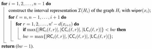

Linear time implementation:  A straightforward implementation gives $O\left({(n+n^{\prime })}^3\right)$ time and $O(n+n^{\prime })$ space algorithm. We here show how to improve the time complexity to linear time. Intuitively, we maintain the differences of three maximum cliques ${\mathsf{LC}}_i$, ${\mathsf{CC}}_i$, and ${\mathsf{RC}}_i$ efficiently, and we use the same idea as in the proof of Theorem 6 twice.

We first fix $i=1$. In this case, we can compute ${\mathsf{LC}}_1$, ${\mathsf{CC}}_1$, and ${\mathsf{RC}}_1$ in $O(n+n^{\prime })$ time; the algorithm first starts ${{\mathsf{RC}}_1}^{\prime }:=\{x_1,y_1,\dots ,y_{n^{\prime }-d\left(x_2\right)}\}$, ${{\mathsf{CC}}_1}^{\prime }:=\{x_1,y_{n^{\prime }-d\left(x_2\right)+1},\dots ,y_{n^{\prime }}\}$, and ${{\mathsf{LC}}_1}^{\prime }:=\{x_2,\dots ,x_n,y_{n^{\prime }-d\left(x_2\right)+1},\dots ,y_{n^{\prime }}\}$. That is, all points in $X_2^R(=\{x_2,\dots ,x_n\})$ are extended to the left, and all points in $Y_2^L(=Y\backslash N\left(x_2\right))$ are extended to the right. If $max\{\left|{{\mathsf{LC}}_1}^{\prime }\right|,\left|{{\mathsf{RC}}_1}^{\prime }\right|\}>\left|{{\mathsf{CC}}_1}^{\prime }\right|$, the algorithm flips the interval (or updates ℓ or r) into ${{\mathsf{CC}}_1}^{\prime }$, decreases $\left|{{\mathsf{LC}}_1}^{\prime }\right|$ or $\left|{{\mathsf{RC}}_1}^{\prime }\right|$, and increases $\left|{{\mathsf{CC}}_1}^{\prime }\right|$. Repeating this process, in $O(n+n^{\prime })$ time, when the algorithm meets $max\{\left|{\mathsf{LC}}_1\right|,\left|{\mathsf{RC}}_1\right|\}=\left|{\mathsf{CC}}_1\right|$ or $max\{\left|{\mathsf{LC}}_1\right|,\left|{\mathsf{RC}}_1\right|\}=\left|{\mathsf{CC}}_1\right|-1$, the value gives the minimum size of the maximum cliques in three parts, or equivalently, gives a minimum completion of $H_1$. When we have a minimum completion of $H_1$, we say this pair $(\ell ,r)$ is the best pair for $H_1$.

Now, we compute ${\mathsf{LC}}_2$, ${\mathsf{CC}}_2$, and ${\mathsf{RC}}_2$ from ${\mathsf{LC}}_1$, ${\mathsf{CC}}_1$, and ${\mathsf{RC}}_1$ with the best pair for $H_1$ in $O(d\left(x_1\right)-d\left(x_3\right))$ time. Intuitively, $H_2$ is obtained from $H_1$ by the following steps; (1) remove $I_{x_2}=[1,1]$ from the point 1, and put it as an interval $[0,d\left(x_1\right)]$; (2) shift all positive points $I_{y_j}$ at $d\left(x_1\right)-j+1$ with $y_j\in N\left(x_1\right)\backslash N\left(x_2\right)$ to $d\left(x_2\right)-j+1$; and (3) remove all intervals $I_{y_j}=[-1,0]$ with $y_j\in N\left(x_2\right)\backslash N\left(x_3\right)$ and put them at $d\left(x_2\right)-j+1$ as points. The movements have influences on ${\mathsf{LC}}_1$, ${\mathsf{CC}}_1$, and ${\mathsf{RC}}_1$, and from them, we construct ${\mathsf{LC}}_2$, ${\mathsf{CC}}_2$, and ${\mathsf{RC}}_2$, and obtain the best pair for $H_2$ in a similar way to that used in the proof of Theorem 6. Then, since $N\left(x_3\right)\subseteq N\left(x_2\right)\subseteq N\left(x_1\right)$, the total difference (or the total number of flipped intervals) can be bounded above by $\left|\left\{x_2\right\}\cup (N\left(x_1\right)\backslash N\left(x_2\right))\cup (N\left(x_2\right)\backslash N\left(x_3\right))\right|=\left|\left\{x_2\right\}\cup (N\left(x_1\right)\backslash N\left(x_3\right))\right|=d\left(x_1\right)-d\left(x_3\right)+1$. Hence the computation of ${\mathsf{LC}}_2$, ${\mathsf{CC}}_2$, and ${\mathsf{RC}}_2$ from ${\mathsf{LC}}_1$, ${\mathsf{CC}}_1$, and ${\mathsf{RC}}_1$ requires $O(d\left(x_1\right)-d\left(x_3\right))$ time.

Repeating this process, the computation of ${\mathsf{LC}}_i$, ${\mathsf{CC}}_i$, ${\mathsf{RC}}_i$, and the best pair of $H_i$ from ${\mathsf{LC}}_{i-1}$, ${\mathsf{CC}}_{i-1}$, and ${\mathsf{RC}}_{i-1}$ with the best pair for $H_{i-1}$ requires $O(d\left(x_{i-1}\right)-d\left(x_{i+1}\right))$ time for each $1<i\le n$. Hence, by maintaining the differences, the total computation time of Algorithm 3 is the sum of the computations of (1) $\mathsf{bw}\left(H_0\right)$, (2) ${\mathsf{LC}}_1$, ${\mathsf{CC}}_1$, ${\mathsf{RC}}_1$, and the best pair of $H_1$, and (3) ${\mathsf{LC}}_i$, ${\mathsf{CC}}_i$, and ${\mathsf{RC}}_i$ with the best pair of $H_i$ from ${\mathsf{LC}}_{i-1}$, ${\mathsf{CC}}_{i-1}$, ${\mathsf{RC}}_{i-1}$, and the best pair of $H_{i-1}$ for $i=2,3,\dots ,n-1$, which is equal to $O(n+n^{\prime })+{\sum }_{i=2}^{n-1}O(d\left(x_{i-1}\right)-d\left(x_{i+1}\right))=O(n+n^{\prime })$.      ■

Here we extend Corollary 7 to a chain graph.

Corollary 10 

For a connected chain graph $G=(X,Y,E)$, we assume that $X=\{x_1,x_2,\dots ,x_n\}$ and $Y=\{y_1,y_2,\dots ,y_{n^{\prime }}\}$ are already ordered by inclusion of neighbors. Then we have an optimal layout that satisfies $X_0<Y_0<X_1\cup Y_1<X_2<Y_2$ such that (1) $X_0=\{x_1,\dots ,x_i\}$, $X_1=\{x_{i+1},\dots ,x_j\}$, and $X_2=\{x_{j+1},\dots ,x_n\}$ for some $1\le i\le j\le n$, and (2) $Y_2=\{y_1,\dots ,y_k\}$, $Y_1=\{y_{k+1},\dots ,y_{\ell }\}$, and $Y_0=\{y_{\ell +1},\dots ,y_{n^{\prime }}\}$ for some $1\le k\le \ell \le n$. Any arrangement of vertices in $X_1\cup Y_1$ gives us an optimal layout. Moreover, the bandwidth is determined by an edge between (1) $X_0$ and $Y_0$, (2) $(X_1\cup X_2)$ and $(Y_0\cup Y_1)$, or (3) $X_2$ and $Y_2$.

Proof. For an optimal layout, we have a corresponding wiper. Then the set $X_0$ is determined by $x_i\in X$ which is the maximum vertex in X not crossing the wiper. Then $Y_0$ is determined by the maximum vertex $y_k$ in $N\left(x_i\right)$. Similarly, the set $Y_2$ is determined by the minimum vertex $y_{\ell }$ not crossing the wiper, and $X_2$ is determined by the minimum vertex in $N\left(y_{\ell }\right)$. Considering the maximum cliques which can give the bandwidth, the corollary follows.      ■

4. Intractable Problems on a (Unit) Grid Intersection Graph

In this section, we turn to the grid intersection graphs and intractable problems for the class.

4.1. The Hamiltonian Cycle Problem

We give two hardness results for grid intersection graphs in this section.

Theorem 11 

The Hamiltonian cycle problem is $\mathcal{NP}$-complete for unit grid intersection graphs.

Proof. It is clear that the problem is in $\mathcal{NP}$. Hence we show $\mathcal{NP}$-hardness. We show a similar reduction in [57]. We start from the Hamiltonian cycle problem in planar directed graph with degree bound two, which is still $\mathcal{NP}$-hard [58]. Let $G_0=(V_0,A)$ be a planar directed graph with degree bound two. (We deal with directed graphs only in this proof; we will use $(u,v)$ as a directed edge, called arc, which is distinguished from $\{u,v\}$.) As shown in [57,58], we can assume that $G_0$ consists of two types of vertices: (type △) with indegree two and outdegree one, and (type ▽) with indegree one and outdegree two. Hence, the set $V_0$ of vertices can be partitioned into two sets $V_{△}$ and $V_{▽}$ that consist of the vertices in type △ and ▽, respectively.

Moreover, we have two more claims; (1) the unique arc from a type △ vertex has to be the unique arc to a type ▽ vertex; and (2) each of two arcs from a type ▽ vertex has to be one of two arcs to a type △ vertex. If the unique arc from a type △ vertex v is into one of a type △ vertex u, the vertex u has to be visited from v to make a Hamiltonian cycle. Hence the vertex u can be replaced by an arc from v to the vertex w which is pointed from u. On the other hand, if one of two arcs from a type ▽ vertex v reaches another type ▽ vertex u, the vertex u should be visited from v. Hence the other arc a from v can be removed from $G_0$. Then the vertex w incident to a has degree 2. Hence we have two cases; w can be replaced by an arc, or we can conclude $G_0$ does not have a Hamiltonian cycle. Repeating these processes, we have the claims (1) and (2), which imply that we have $\left|V_{△}\right|=\left|V_{▽}\right|$, the underlying graph of $G_0$ is bipartite (with two sets $V_{△}$ and $V_{▽}$), and any cycle contains two types of vertices alternately.

By the claims, we can partition arcs into two groups; (1) arcs from a type △ vertex to a type ▽ vertex called thick arcs, and (2) arcs from a type ▽ vertex to a type △ vertex called thin arcs. By above discussion, we can observe that any Hamiltonian cycle has to contain all thick arcs (Moreover, contracting thick arcs, we can show $\mathcal{NP}$-completeness of the Hamiltonian cycle problem even if we restrict ourselves to the directed planar graphs that only consist of vertices of two outdegrees and two indegrees.)

Now, we construct a unit grid intersection graph $G_1=(V_1,E_1)$ from $G_0=(V_0,A)$ which satisfies the above conditions. One type ▽ vertex is represented by five vertical lines and two horizontal lines, and one type △ vertex is represented by three vertical lines and one horizontal line in Figure 4 (each corresponding line segments are in gray area). Each thick arc is represented by alternations of one parallel vertical line and one parallel horizontal line in Figure 4, and each thin arc is represented by alternations of two parallel vertical lines and two parallel horizontal lines in Figure 5. The vertices are joined by the arcs in a natural way. An example is illustrated in Figure 6.

Figure 4. Reduction of thick arcs.

Figure 4. Reduction of thick arcs.

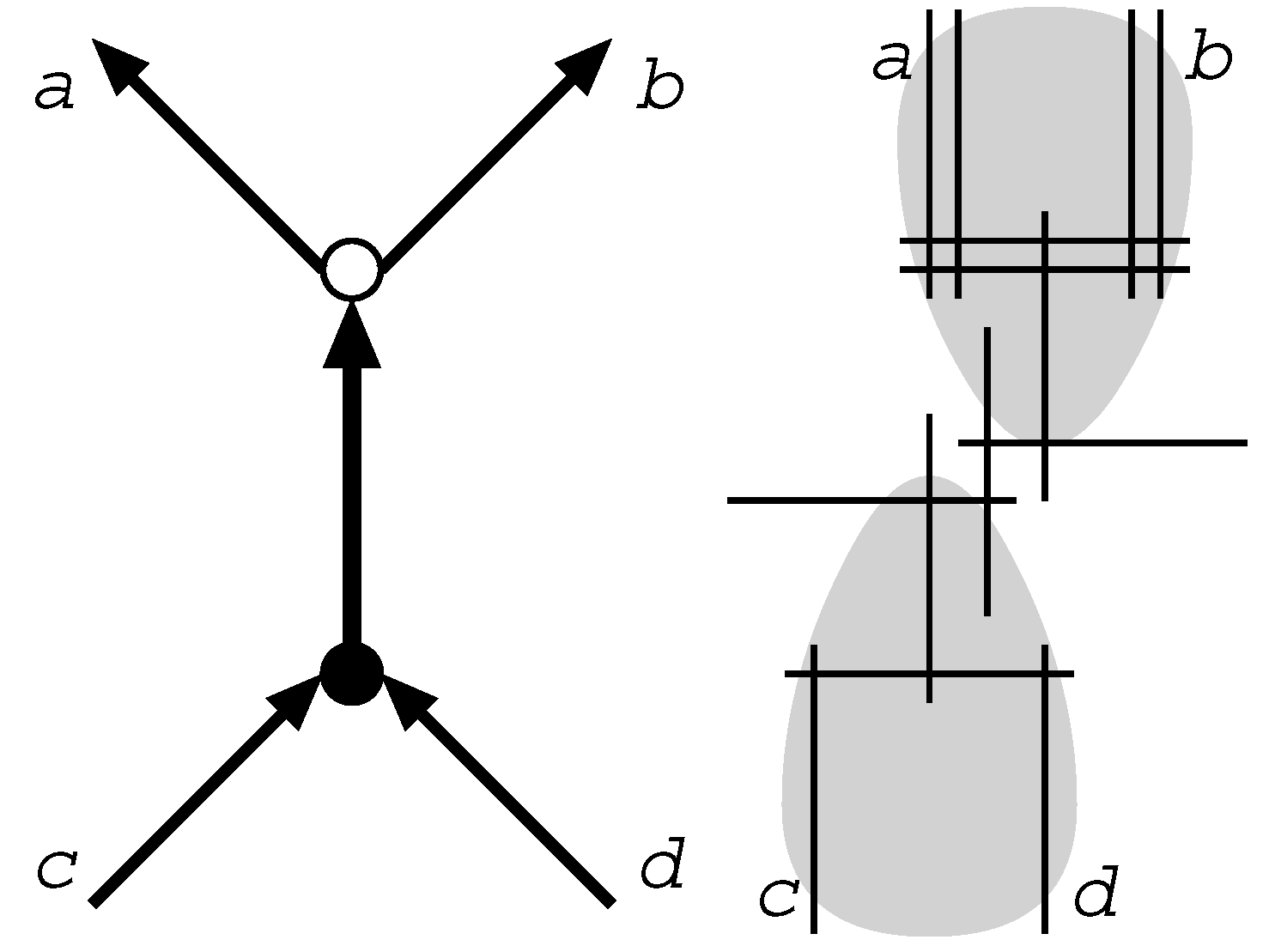
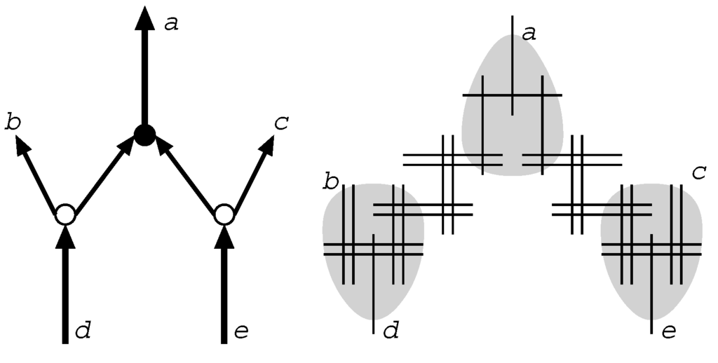
Figure 5. Reduction of thin arcs.

Figure 5. Reduction of thin arcs.

Figure 6. Reduction of a graph $G_0$.

Figure 6. Reduction of a graph $G_0$.

For the resultant graph $G_1$, it is obvious that the reduction can be done in a polynomial time, and $G_1$ is a unit grid intersection graph. Hence we show $G_0$ has a Hamiltonian cycle if and only if $G_1$ has a Hamiltonian cycle. First, we assume that $G_0$ has a Hamiltonian cycle $C_0$, and show that $G_1$ also has a Hamiltonian cycle $C_1$. $C_1$ visits the vertices (or line segments) in $G_1$ along $C_0$ as follows. For each thick arc in $G_0$, the corresponding segments in $G_1$ are visited straightforwardly. We show how to visit the segments corresponding to thin arcs (Figure 7). For each thin arc not on $C_0$, they are visited by $C_1$ as shown in the left side of Figure 7 (between u and v); a pair of parallel lines are used to sweep the arc twice, and the endpoints are joined by one line segment in the gadget of a type △ vertex (v). On the other hand, for each thin arc on $C_0$, they are visited by $C_1$ as shown in the right side of Figure 7 (between w and v); a pair of parallel lines are used to sweep the arc once, and the path goes from e to a. Hence from a given Hamiltonian cycle $C_0$ on $G_0$, we can construct a Hamiltonian cycle $C_1$ on $G_1$.

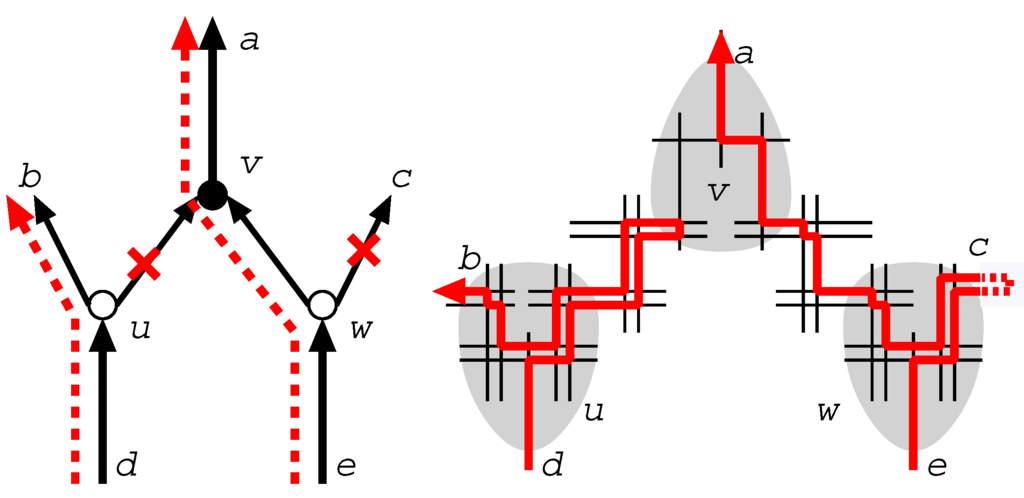
Figure 7. How to sweep thin arcs.

Figure 7. How to sweep thin arcs.

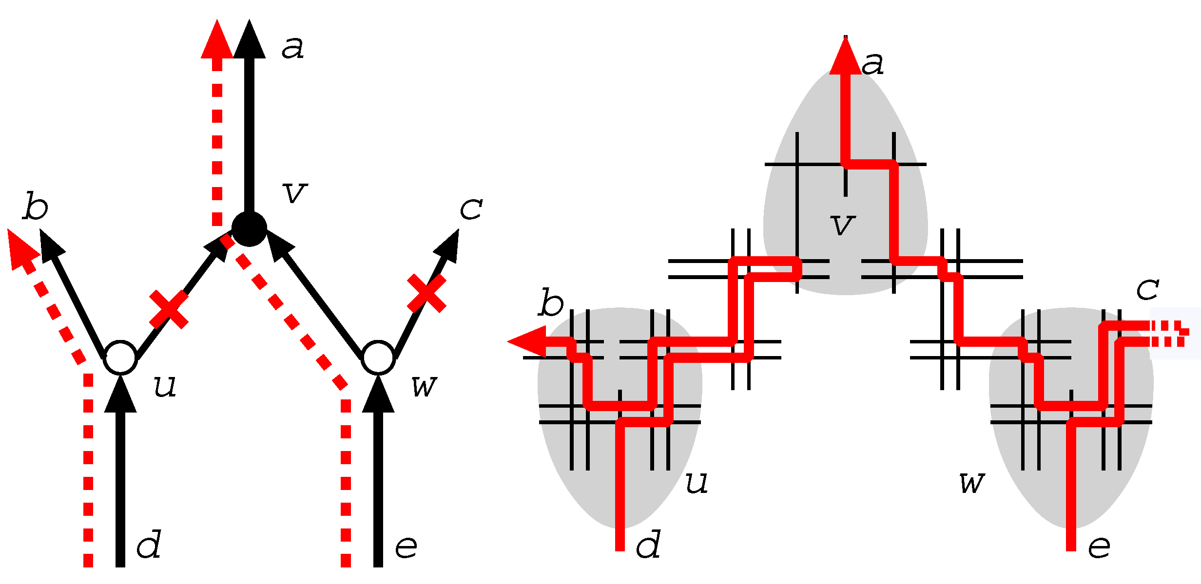
Now we assume that $G_1$ has a Hamiltonian cycle $C_1$, and show that $G_0$ also has a Hamiltonian cycle $C_0$. By observing that there are no ways for $C_1$ to visit lines corresponding to thick arcs described above, and the unique center horizontal line of a type △ vertex can be used exactly once, we can see that $C_1$ forms a Hamiltonian cycle of $G_1$ as in the same manner represented above. Hence $C_0$ can be constructed from $C_1$ in the same way. ■     ■

Corollary 12 

The Hamiltonian path problem is $\mathcal{NP}$-complete for unit grid intersection graphs.

Proof. We reduce the graph $G_1$ in the proof of Theorem 11 to $G_1^{\prime }$ as follows; pick up any line segment in a thick arc, and add one more line segment as in Figure 8. Then, it is easy to see that $G_1$ has a Hamiltonian cycle if and only if $G_1^{\prime }$ has a Hamiltonian path (with an endpoint corresponding to the additional line segment). Hence we have the corollary. ■     ■

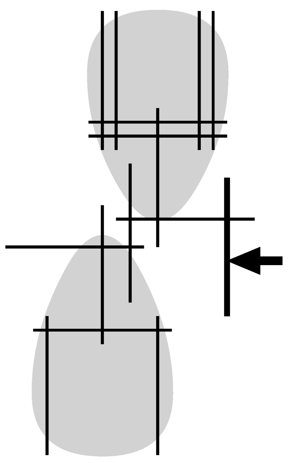
Figure 8. Hamiltonian path problem.

Figure 8. Hamiltonian path problem.

4.2. The Graph Isomorphism Problem

Theorem 13 

The graph isomorphism problem is $GI$-complete for grid intersection graphs.

Proof. We show a similar reduction in [38,54]. We start by considering the graph isomorphism problem for general graphs. Let $G_0=(V_0,E_0)$ and $G_0^{\prime }=(V_0^{\prime },E_0^{\prime })$ with $\left|V_0\right|=\left|V_0^{\prime }\right|=n$ and $\left|E_0\right|=\left|E_0^{\prime }\right|=m$ be an instance of the graph isomorphism problem. (We will refer the graph $G_0$ in Figure 9(1) as an example). Without loss of generality, we assume that $G_0$ is connected. From $G_0$, we define a bipartite graph $G_1=(V_0,E_0,E_1)$ with two vertex sets $V_0$ and $E_0$ by $E_1:=\{\{v,e\}\mid v \mathrm{i}\mathrm{s} \mathrm{o}\mathrm{n}\mathrm{e} \mathrm{e}\mathrm{n}\mathrm{d}\mathrm{p}\mathrm{o}\mathrm{i}\mathrm{n}\mathrm{t} \mathrm{o}\mathrm{f} e\}$. (Intuitively, each edge is divided into two edges joined by a new vertex; see Figure 9(2)). Then, $e\in E_0$ have degree 2 by its two endpoints in $V_0$. It is easy to see that $G_0\sim G_0^{\prime }$ if and only if $G_1\sim G_1^{\prime }$ for any graphs $G_0$ and $G_0^{\prime }$ with resultant graphs $G_1$ and $G_1^{\prime }$.

Figure 9. Reduction for $GI$-completeness.

Figure 9. Reduction for $GI$-completeness.

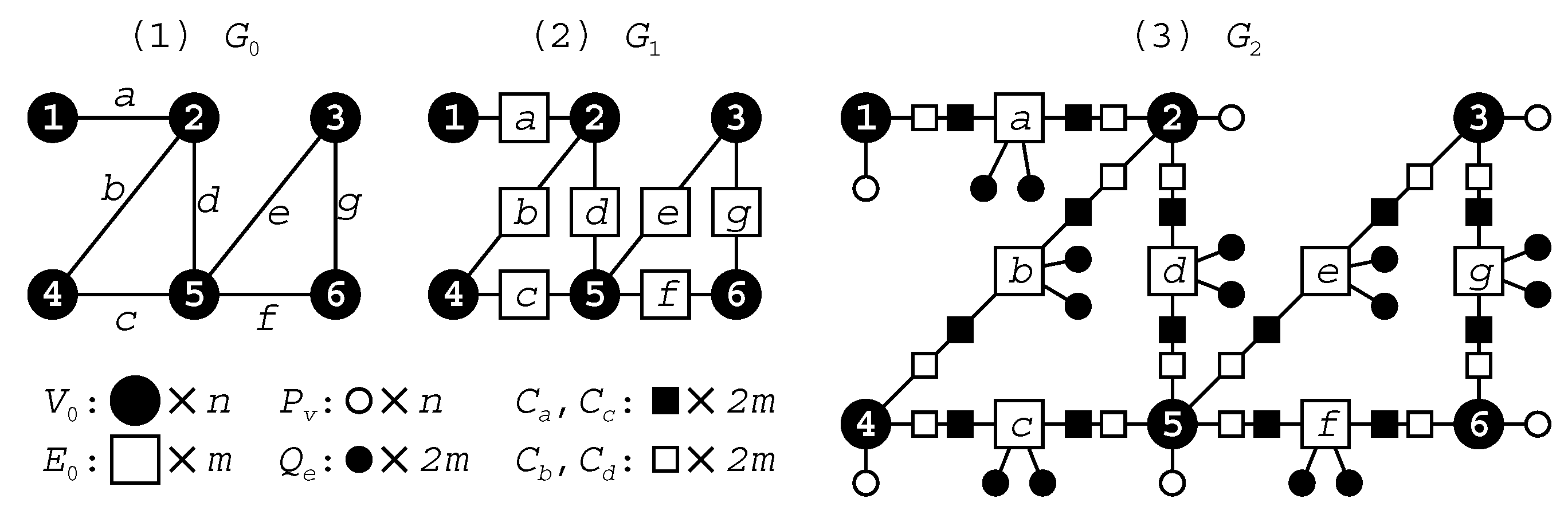
Now, we construct a grid intersection graph $G_2=(V_2,E_2)$ from the bipartite graph $G_1=(V_0,E_0,E_1)$ such that $G_1\sim G_1^{\prime }$ if and only if $G_2\sim G_2^{\prime }$ in the same manner. The vertex set $V_2$ consists of the following sets (see Figure 9(3)):

• $V_0$, $E_0$; we let $V_0=\{v_1,v_2,\dots ,v_n\}$, $E_0=\{e_1,e_2,\dots ,e_m\}$, where $e_i=\{v_i,v_j\}$ for some $1\le i,j\le n$.
• $P_v,Q_e$; each vertex in $P_v\cup Q_e$ is called pendant and $P_v:=\{p_1,p_2,\dots ,p_n\}$, $Q_e:=\{q_1,q_2,\dots ,q_m,q_1^{\prime },q_2^{\prime },\dots ,q_m^{\prime }\}$. That is, we have $\left|P_v\right|=n$ and $\left|Q_e\right|=2m$.
• $C_a,C_b,C_c,C_d$; each vertex in $C_a\cup C_b\cup C_c\cup C_d$ is called connector, and $C_a:=\{a_1,a_2,\dots ,a_m\}$, $C_b:=\{b_1,b_2,\dots ,b_m\}$, $C_c:=\{c_1,c_2,\dots ,c_m\}$, and $C_d:=\{d_1,d_2,\dots ,d_m\}$.

The edge set $E_2$ contains the following edges (Figure 9(3)):

• For each i with $1\le i\le n$, each pendant $p_i$ is joined to $v_i$. That is, $\{p_i,v_i\}\in E_2$ for each i with $1\le i\le n$.
• For each j with $1\le j\le m$, two pendants $q_j$ and $q_j^{\prime }$ are joined to $e_j$. That is, $\{q_j,e_j\},\{q_j^{\prime },e_j\}\in E_2$ for each j with $1\le j\le m$.
• For each $e_j$ with $1\le j\le m$, we have two vertices $v_i$ and $v_{i^{\prime }}$ with $\{v_i,e_j\},\{v_{i^{\prime }},e_j\}\in E_1$. For the three vertices $e_j$, $v_i$, $v_{i^{\prime }}$, we add $\{e_j,a_j\}$, $\{v_i,b_j\}$, $\{a_j,b_j\}$, $\{e_j,c_j\}$, $\{v_{i^{\prime }},d_j\}$, $\{c_j,d_j\}$ into $E_2$. Intuitively, each edge in $G_1$ is replaced by a path of length 3 that consists of one vertex in $C_a\cup C_c$ and the other one in $C_b\cup C_d$.

The edge set $E_2$ also contains the edges $\{v_i,e_j\}$ for each $i,j$ with $1\le i\le n$ and $1\le j\le m$. In other words, every vertex in $V_0$ is connected to all vertices in $E_0$ (the edges are omitted in Figure 9(3) to simplify).

Let $G_0$ and $G_0^{\prime }$ be any two graphs. Then, it is easy to see that $G_0\sim G_0^{\prime }$ implies $G_2\sim G_2^{\prime }$. Hence, we have to show that $G_2$ is a grid intersection graph, and $G_0$ can be reconstructed from $G_2$ uniquely up to isomorphism.

We can represent the vertices in $V_0\cup Q_e\cup C_a\cup C_c$ (white vertices in Figure 9(3)) as horizontal segments and the vertices in $E_0\cup P_v\cup C_b\cup C_d$ (black vertices in Figure 9(3)) as vertical segments as follows (Figure 10): First, all vertices in $V_0$ correspond to unit length horizontal segments that are placed in parallel. All vertices in $E_0$ correspond to unit length vertical segments placed in parallel, and the segments corresponding to vertices in $V_0$ and $E_0$ make a mesh structure (as in Figure 10). Each pendant vertex in $P_v$ and $Q_e$ corresponds to a short segment, and is attached to its neighbor in an arbitrary way, for example, as in Figure 10. Each pair of connectors in $C_a$ and $C_b$ (or $C_c$ and $C_d$) joins corresponding vertices in $V_0$ and $E_0$ as in Figure 10. Then it is easy to see that the resultant grid representation gives $G_2$.

Next, we show that $G_0$ can be reconstructed from $G_2$ uniquely up to isomorphism. First, any vertex of degree 1 is a pendant in $G_2$. Hence we can distinguish $P_v\cup Q_e$ from the other vertices. Then, for each vertex $v\in V_2\backslash (P_v\cup Q_e)$, $\left|N\left(v\right)\cap (P_v\cup Q_e)\right|=1$ if and only if $v\in V_0$, and $\left|N\left(v\right)\cap (P_v\cup Q_e)\right|=2$ if and only if $v\in E_0$. Hence two sets $V_0$ and $E_0$ are distinguished, and then $P_v\cup Q_e$ can be divided into $P_v$ and $Q_e$. Moreover, we have $C_a\cup C_b\cup C_c\cup C_d=V_2\backslash (P_v\cup Q_e\cup V_0\cup E_0)$. Thus, tracing the paths induced by $C_a\cup C_b\cup C_c\cup C_d$, we can reconstruct each edge $e_j=(v_i,v_{i^{\prime }})$ with $e_j\in E_0$ and $v_i,v_{i^{\prime }}\in V_0$. Therefore, we can reconstruct $G_0$ from $G_2$ uniquely up to isomorphism.

Hence the graph isomorphism problem for grid intersection graphs is as hard as the graph isomorphism problem for general graphs. Thus the graph isomorphism problem is $GI$-complete for grid intersection graphs. ■     ■

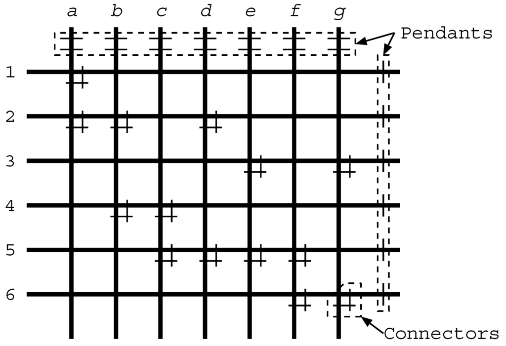
Figure 10. Grid representation of $G_2$.

Figure 10. Grid representation of $G_2$.

5. Conclusions

In this paper, we focus on geometrical intersection graphs. From the viewpoint of the parameterized complexity (see Downey and Fellow [59]), it is interesting to investigate efficient algorithms for these graph classes with some constraints. What if the number of vertical lines (or the possible positions on the coordinate of vertical lines) is bounded by a constant? In this case, we can use the dynamic programming technique for the graphs. Do the restrictions make some intractable problems solvable in polynomial time? From the graph theoretical point of view, a geometric model for chordal bipartite graphs is open. It is pointed out by Spinrad in [60], but it is not solved yet. The graph isomorphism problem for unit grid intersection graphs is also interesting. By Theorem 13, the graph isomorphism problem is $GI$-complete for grid intersection graphs. In the proof, we only need two kinds of lengths—long line segments and short line segments, but the difference of these two lengths is essential in the proof, and we cannot make all line segments unit length in the reduction.

References

- Golumbic, M. Algorithmic Graph Theory and Perfect Graphs, 2nd ed.; Elsevier: Amsterdam, The Netherlands, 2004. [Google Scholar]
- Spinrad, J. Efficient Graph Representations; American Mathematical Society: Providence, RI, USA, 2003. [Google Scholar]
- Fishburn, P.C. Interval Orders and Interval Graphs; Wiley & Sons, Inc.: Hoboken, NJ, USA, 1985. [Google Scholar]
- McKee, T.; McMorris, F. Topics in Intersection Graph Theory; SIAM: Philadelphia, PA, USA, 1999. [Google Scholar]
- Uehara, R. Simple Geometrical Intersection Graphs. In Proceedings of the Workshop on Algorithms and Computation (WALCOM 2008); Springer-Verlag: Berlin/Heidelberg, Germany, 2008; pp. 25–33. [Google Scholar]
- Uehara, R. Bandwidth of Bipartite Permutation Graphs. In Proceedings of the Annual International Symposium on Algorithms and Computation (ISAAC 2008); Springer-Verlag: Berlin/Heidelberg, Germany, 2008; pp. 824–835. [Google Scholar]
- Lai, Y.L.; Williams, K. A survey of solved problems and applications on bandwidth, edgesum, and profile of graphs. J. Graph Theory 1999, 31, 75–94. [Google Scholar] [CrossRef]
- Chinn, P.Z.; Chvátalová, J.; Dewdney, A.K.; Gibbs, N.E. The bandwidth problem for graphs and matrices—A survey. J. Graph Theory 1982, 6, 223–254. [Google Scholar] [CrossRef]
- Kaplan, H.; Shamir, R. Pathwidth, bandwidth, and completion problems to proper interval graphs with small cliques. SIAM J. Comput. 1996, 25, 540–561. [Google Scholar] [CrossRef]
- Kaplan, H.; Shamir, R.; Tarjan, R. Tractability of parameterized completion problems on chordal, strongly chordal, and proper interval graphs. SIAM J. Comput. 1999, 28, 1906–1922. [Google Scholar] [CrossRef]
- Papadimitriou, C.H. The NP-completeness of the bandwidth minimization problem. Computing 1976, 16, 263–270. [Google Scholar] [CrossRef]
- Garey, M.; Johnson, D. Computers and Intractability—A Guide to the Theory of NP-Completeness; Freeman: Gordonsville, VA, USA, 1979. [Google Scholar]
- Monien, B. The bandwidth minimization problem for caterpillars with hair length 3 is NP-complete. SIAM J. Alg. Disc. Meth. 1986, 7, 505–512. [Google Scholar] [CrossRef]
- Kloks, T.; Kratsch, D.; Borgne, Y.L.; Müller, H. Bandwidth of Split and Circular Permutation Graphs. In Proceedings of the WG 2000; Springer-Verlag: Berlin/Heidelberg, Germany, 2000; pp. 243–254. [Google Scholar]
- Shrestha, A.M.S.; Tayu, S.; Ueno, S. Bandwidth of Convex Bipartite Graphs and Related Graphs. In Proceedings of the COCOON 2011; Springer-Verlag: Berlin/Heidelberg, Germany, 2011; pp. 307–318. [Google Scholar]
- Feige, U. Coping with the NP-Hardness of the Graph Bandwidth Problem. In Proceedings of the 7th Scandinavian Workshop on Algorithm Theory (SWAT 2000); Springer-Verlag: Berlin/Heidelberg, Germany, 2000; pp. 10–19. [Google Scholar]
- Cygan, M.; Pilipczuk, M. Exact and approximate bandwidth. Theor. Comput. Sci. 2010, 411, 3701–3713. [Google Scholar] [CrossRef]
- Cygan, M.; Pilipczuk, M. Even faster exact bandwidth. ACM Trans. Algorithm 2012, 8, 1–14. [Google Scholar] [CrossRef]
- Cygan, M.; Pilipczuk, M. Bandwidth and distortion revisited. Discrete Appl. Math. 2012, 160, 494–504. [Google Scholar] [CrossRef]
- Haralambides, J.; Makedon, F.; Monien, B. Bandwidth minimization: An approximation algorithm for caterpillars. Theory Comput. Syst. 1991, 24, 169–177. [Google Scholar] [CrossRef]
- Kloks, T.; Kratsch, D.; Müller, H. Approximating the bandwidth for asteroidal triple-free graphs. J. Algorithm 1999, 32, 41–57. [Google Scholar] [CrossRef]
- Karpinski, M.; Wirtgen, J.; Zelikovsky, A. An Approximation Algorithm for the Bandwidth Problem on Dense Graphs. TR-97-017, Electronic Colloquium on Computational Complexity (ECCC). 1997. Available online: http://eccc.hpi-web.de/report/1997/017/ (accessed on 24 January 2013).
- Gupta, A. Improved bandwidth approximation for trees and chordal graphs. J. Algorithm 2001, 40, 24–36. [Google Scholar] [CrossRef]
- Kloks, T.; Kratsch, D.; Müller, H. Bandwidth of chain graphs. Inf. Process. Lett. 1998, 68, 313–315. [Google Scholar] [CrossRef]
- Kloks, T.; Tan, R.B. Bandwidth and topological bandwidth of graphs with few P4’s. Discrete Appl. Math. 2001, 115, 117–133. [Google Scholar] [CrossRef]
- Kleitman, D.; Vohra, R. Computing the Bandwidth of Interval Graphs. SIAM J. Disc. Math. 1990, 3, 373–375. [Google Scholar] [CrossRef]
- Mahesh, R.; Rangan, C.P.; Srinivasan, A. On finding the minimum bandwidth of interval graphs. Inf. Comput. 1991, 95, 218–224. [Google Scholar] [CrossRef]
- Sprague, A. An O(nlogn) algorithm for bandwidth of interval graphs. SIAM J. Discrete Math. 1994, 7, 213–220. [Google Scholar] [CrossRef]
- Heggernes, P.; Kratsch, D.; Meister, D. Bandwidth of bipartite permutation graphs in polynomial time. J. Discret. Algorithm 2009, 7, 533–544. [Google Scholar] [CrossRef]
- Kratsch, D. Finding the minimum bandwidth of an interval graph. Inf. Comput. 1987, 74, 140–158. [Google Scholar] [CrossRef]
- Booth, K.; Lueker, G. Testing for the consecutive ones property, interval graphs, and graph planarity using PQ-tree algorithms. J. Comput. Syst. Sci. 1976, 13, 335–379. [Google Scholar] [CrossRef]
- Lueker, G.; Booth, K. A linear time algorithm for deciding interval graph isomorphism. J. ACM 1979, 26, 183–195. [Google Scholar] [CrossRef]
- Brandstädt, A.; Lozin, V. On the linear structure and clique-width of bipartite permutation graphs. Ars Comb. 2003, 67, 273–281. [Google Scholar]
- Uehara, R.; Valiente, G. Linear structure of bipartite permutation graphs with an application. Inf. Process. Lett. 2007, 103, 71–77. [Google Scholar] [CrossRef]
- Otachi, Y.; Okamoto, Y.; Yamazaki, K. Relationships between the class of unit grid intersection graphs and other classes of bipartite graphs. Discrete Appl. Math. 2007, 155, 2383–2390. [Google Scholar] [CrossRef]
- Keil, J. Finding hamiltonian circuits in interval graphs. Inf. Process. Lett. 1985, 20, 201–206. [Google Scholar] [CrossRef]
- Müller, H. Hamiltonian circuit in chordal bipartite graphs. Discret. Math. 1996, 156, 291–298. [Google Scholar] [CrossRef]
- Uehara, R.; Toda, S.; Nagoya, T. Graph isomorphism completeness for chordal bipartite graphs and strongly chordal graphs. Discret. Appl. Math. 2004, 145, 479–482. [Google Scholar] [CrossRef]
- Wu, T.H. An O(n3) isomorphism test for circular-arc graphs. Ph.D. Thesis, Applied Mathematics and Statistics, SUNY-Stonybrook, New York, NY, USA, 1983. [Google Scholar]
- Eschen, E.M. Circular-arc graph recognition and related problems. Ph.D. Thesis, Department of Computer Science, Vanderbilt University, Nashville, TE, USA, 1997. [Google Scholar]
- Hsu, W.L. O(M·N) Algorithms for the recognition and isomorphism problem on circular-arc graphs. SIAM J. Comput. 1995, 24, 411–439. [Google Scholar] [CrossRef]
- Curtis, A.R.; Lin, M.C.; McConnell, R.M.; Nussbaum, Y.; Soulignac, F.J.; Spinrad, J.P.; Szwarcfiter, J.L. Isomorphism of graph classes related to the circular-ones property. arXiv:1203.4822v1.
- Roberts, F.S. Indifference Graphs. In Proof Techniques in Graph Theory; Harary, F., Ed.; Academic Press: Waltham, MA, USA, 1969; pp. 139–146. [Google Scholar]
- Bogart, K.P.; West, D.B. A short proof that “proper=unit”. Discret. Math. 1999, 201, 21–23. [Google Scholar] [CrossRef]
- Deng, X.; Hell, P.; Huang, J. Linear-time representation algorithms for proper circular-arc graphs and proper interval graphs. SIAM J. Comput. 1996, 25, 390–403. [Google Scholar] [CrossRef]
- Uehara, R.; Uno, Y. On computing longest paths in small graph classes. Int. J. Found. Comput. Sci. 2007, 18, 911–930. [Google Scholar] [CrossRef]
- Saitoh, T.; Otachi, Y.; Yamanaka, K.; Uehara, R. Random Generation and Enumeration of Bipartite Permutation Graphs. In Proceedings of the 20th International Symposium on Algorithms and Computation (ISAAC 2009); Springer-Verlag: Berlin/Heidelberg, Germany, 2009; pp. 1104–1113. [Google Scholar]
- Brandstädt, A.; Le, V.; Spinrad, J. Graph Classes: A Survey; SIAM: Philadelphia, PA, USA, 1999. [Google Scholar]
- Müller, H. Recognizing interval digraphs and interval bigraphs in polynomial time. Disc. Appl. Math. 1997, 78, 189–205. Available online: http://www.comp.leeds.ac.uk/hm/pub/node1.html (accessed on 22 January 2013). [Google Scholar] [CrossRef]
- Hell, P.; Huang, J. Interval bigraphs and circular Arc graphs. J. Graph Theory 2004, 46, 313–327. [Google Scholar] [CrossRef]
- Rafiey, A. Recognizing interval bigraphs using forbidden patterns. Unpublished work. 2012. [Google Scholar]
- Uehara, R. Canonical Data Structure for Interval Probe Graphs. In Proceedings of the 15th Annual International Symposium on Algorithms and Computation (ISAAC 2004); Lecture Notes in Computer Science Volume 3341. Springer-Verlag: Berlin/Heidelberg, Germany, 2004; pp. 859–870. [Google Scholar]
- Colbourn, C. On testing isomorphism of permutation graphs. Networks 1981, 11, 13–21. [Google Scholar] [CrossRef]
- Babel, L.; Ponomarenko, I.; Tinhofer, G. The isomorphism problem for directed path graphs and for rooted directed path graphs. J. Algorithm 1996, 21, 542–564. [Google Scholar] [CrossRef]
- Nakano, S.-I.; Uehara, R.; Uno, T. A New Approach to Graph Recognition and Applications to Distance Hereditary Graphs. In Proceedings of the 4th Annual Conference on Theory and Applications of Models of Computation (TAMC 07); Springer-Verlag: Berlin/Heidelberg, Germany, 2007; pp. 115–127. [Google Scholar]
- Knuth, D. Sorting and Searching. In The Art of Computer Programming, 2nd ed.; Addison-Wesley Publishing Company: Boston, MA, USA, 1998. [Google Scholar]
- Uehara, R.; Iwata, S. Generalized Hi-Q is NP-Complete. Trans. IEICE 1990, E73, 270–273. Available online: http://www.jaist.ac.jp/˜uehara/pdf/phd7.ps.gz (accessed on 22 January 2013). [Google Scholar]
- Plesník, J. The NP-completeness of the hamiltonian cycle problem in planar digraphs with degree bound two. Inf. Process. Lett. 1979, 8, 199–201. [Google Scholar] [CrossRef]
- Downey, R.; Fellows, M. Parameterized Complexity; Springer: Berlin/Heidelberg, Germany, 1999. [Google Scholar]
- Spinrad, J. Open Problem List. 1995. Available online: http://www.vuse.vanderbilt.edu/~spin/open.html (accessed on 22 January 2013).
© 2013 by the authors; licensee MDPI, Basel, Switzerland. This article is an open access article distributed under the terms and conditions of the Creative Commons Attribution license (http://creativecommons.org/licenses/by/3.0/).