Grey Target Group Decision Making Based on Three-Parameter Interval Grey Numbers and Bidirectional Projection Method

Abstract

To address the grey target group decision-making method (GDMM) concerning the aggregation of decision-maker information and the approach to ranking alternatives via bidirectional projection (BP), this paper develops a novel methodological framework that optimizes both information integration and alternative evaluation, where a new transformation mechanism between the three-parameter interval grey number (TPIGN) and dual connection number (CN) is established by integrating an induced TPIGN weighted average (ITPIGN-WA) operator with an improved bidirectional projection method (IBPM). The results confirm that the new framework leads to more reliable and effective group decision making (GDM). The new TPIGN conversion mechanism and the set pair potential (SPP)-based ITPIGN-WA better captures decision-maker preferences than previous operators, and the introduction of the IBPM further refines alternative ranking. This dual innovation enriches the theoretical system of grey target decision making and provides significant applied value for enhancing the quality and effectiveness of GDM processes in uncertain environments.

1. Introduction

Grey theory was founded by Professor Deng Julong in 1982. Its core lies in uncovering the evolutionary patterns of systems through limited information, demonstrating particular strength in addressing uncertain systems characterized by a “small sample and poor information.” It has exhibited unique value across numerous fields, such as agriculture, industry, and energy environments. In recent years, the theory has continued to expand into emerging areas, including health care, transportation, and information security. Furthermore, it has integrated with neural networks and fuzzy mathematics to form grey hybrid models, significantly enhancing decision support capabilities for complex systems. Today, it has become an important tool for tackling uncertainty-related problems [1,2].

Among its methodologies, grey target decision making is one of the approaches used to solve multi-criteria decision-making problems. The basic idea is to identify, within a set of pattern sequences, the data that best approximate the target value of a sub-proposition based on the requirements of the given proposition’s information source, especially when the decision model contains grey elements. In practical application, each sequence and the reference sequence together form a grey target, with the reference sequence serving as the bullseye (BE). The distance between each sequence and the BE is called the bullseye distance (BED), and alternatives are ranked according to the magnitude of this distance.

The grey target decision-making method has garnered significant attention from numerous scholars and has undergone gradual refinement and expansion. Liu S.F. employed Euclidean distance to define the BED in grey target decision making and constructed an S-dimensional spherical grey target decision-making model [3]. Song Jie et al. extended the spherical grey target to an ellipsoidal grey target with both positive and negative BE by defining these dual reference points, thereby establishing a positive–negative BE grey target model [4]. Liu Zhongxia et al. further expanded the concept of interval numbers and developed a generalized grey target decision-making ranking method based on a BP consistency coefficient with positive and negative BE [5].

In the process of grey target GDM, considering the complexity and uncertainty of objective matters, decision makers often provide evaluation information in the form of interval numbers. When a two-parameter interval number represents a parameter, it is assumed that values within the entire interval are equally probable, which can lead to significant errors in the calculation results [6]. To address this limitation of interval numbers, Bu Guangzhi et al. first proposed representing grey information using three-parameter interval numbers and provided corresponding definitions and operational rules [7]. Building on this, Luo Dang clarified the definition of TPIGN and conducted research on multi-attribute decision-making techniques using this [8]. Considering the influence of decision makers’ satisfaction ranges for criteria and their risk attitudes for GDM, Yan et al. proposed a TPIGN-based grey target GDMM grounded in prospect theory [9]. In response to the uncertainty of decision information, LI and Yuan introduced a decision-making method based on a projection model using TPIGN linguistic variables [10]. Wang Xia addressed decision-making problems involving interval number (IN) and TPIGN separately. She defined positive and negative BED from each alternative to the positive ideal solutions (PIS) and negative ideal solutions (NIS), respectively, and defined comprehensive BED for the alternatives from different perspectives, ultimately ranking the alternatives based on the magnitude of these comprehensive distances [11]. Ye, L et al. proposed a multi-attribute grey target GDMM based on TPIGN, taking into account both the value information of these numbers and the risk attitudes of the decision makers [12]. In summary, the advances in grey target decision making are primarily reflected in the information representation and ranking methods, as shown in Table 1.

Table 1. Literature classification table for grey target decision making.

Information Type	Sorting Method	Literature
IN	Calculate BED for direct alternative ranking	Liu and Lin, 2010 [3]
	Calculate positive and negative BED for alternative ranking	SONG et al., 2010 [4]
	Utilize bidirectional projection method for alternative ranking	LIU et al., 2019 [5]
TPIGN	Comprehensive BED for alternative ranking	LUO, 2009 [8]
	Rank alternatives based on comprehensive prospect value	YAN et al., 2015 [9]
	Utilize unidirectional projection method for alternative ranking	LI and YUAN, 2017 [10]
	Utilize relative BED and comprehensive BED for alternative ranking	WANG, 2017 [11]
	Rank alternatives based on relative BED to positive and negative BE	YE and ZHANG, 2020 [12]

In the process of grey target GDMM, once INs are adopted to represent the characteristic behavior of objects, the aggregation of decision makers’ information becomes the primary issue to be addressed [13]. Information aggregation primarily relies on various operators. Among these, the ordered weighted averaging (OWA) operator, proposed by American scholar Yager in 1988, is an information aggregation method that lies between the maximum and minimum operators [14]. It has been widely applied in numerous fields, such as artificial intelligence and group decision analysis [15]. In 1999, Yager extended the OWA operator and introduced the induced ordered weighted averaging (IOWA) operator. The IOWA operator integrates data information through an induced variable, which primarily reflects the decision maker’s attitude or the precision of the decision information [16]. To aggregate the IN, Yager further proposed a continuous ordered weighted averaging (COWA) operator. This operator can not only aggregate the IN into a real number form but also incorporate an attitude parameter to directly reflect the optimism level of the decision maker in providing evaluation information [17]. Based on this, Xu Zeshui extended the COWA operator, proposing the weighted COWA operator, the ordered weighted COWA operator, and the combined COWA operator [18]. Wang Xinfan provided definitions for the continuous TPIGN ordered weighted averaging (CTP-OWA) operator and the continuous TPIGN ordered weighted geometric (CTP-OWG) operator. Furthermore, he proposed the weighted CTP-OWA operator and the weighted CTP-OWG operator, establishing an uncertain multi-attribute decision-making method based on these operators [19]. The target objects addressed by the aforementioned aggregation operators are presented in Table 2.

Table 2. Literature classification table for aggregation operators.

Information Type	Operator Name	Literature
Real Number	OWA operator, an information aggregation method between the maximum and minimum operators	Yager, 1988 [14] Zhou et al., 2012 [15]
IN	IOWA operator, integrates data information through an induced variable	Yager, 1999 [16]
	COWA operator, aggregates interval numbers into real numbers	Yager, 2006 [17]
	weighted COWA operator, ordered weighted COWA operator, and combined COWA operator	Xu, 2005 [18]
TPIGN	CTP-OWA operator, CTP-OWG operator, weighted CTP-OWA operator, and weighted CTP-OWG operator	Wang, 2008 [19]

From Table 2, it can be observed that aggregation operators are all based on the premise of ordered data. Therefore, how to achieve a reasonable ordering of IN becomes the primary problem to be solved for information aggregation. The emergence of set pair theory provides a completely new approach for ordering IN. Proposed by Zhao Keqin in 1989, set pair theory is an uncertainty analysis method based on the dialectical principle of the unity of opposites, and it has achieved significant development to date [20]. The CN, as the main tool of set pair theory, on one hand links a determinable number with its range, and on the other hand dynamically connects the deterministic quantity at the macro level with the uncertain quantity at the micro level. Many scholars have converted IN into CN to achieve multi-attribute decision making, yielding numerous results [21]. Among these, the SPP of the connection number has received considerable attention because it can effectively reflect a certain trend of connection between two sets under a specified problem background. Consequently, after converting IN into CN, using the SPP of the connection number to achieve the ordering of IN is a feasible approach.

Furthermore, as another key research focus in grey target GDMM, the ranking of alternatives has been extensively studied in various application scenarios using the BP method [22,23]. Notably, WANG and JING compared the BP method with the unidirectional and orthogonal projection methods, demonstrating its superiority, while HU et al. improved the vector modulus formula and presented a BP method under probabilistic linguistic information. These studies collectively validate the advantages of the BP method in alternative ranking.

Based on the aforementioned background, this paper presents the following research:

(1)

Existing TPIGN aggregation methods primarily focus on information itself, overlooking systematic characterization of certainty–uncertainty relationships among items. This study first introduces the “SPP” concept to quantify the internal situational structure of the grey number (GN), thereby constructing weights. This approach enhances the aggregation mechanism by addressing the underlying logic of information relationships. Consequently, the ITPIGN-WA operator not only aggregates information but also reflects its internal certainty and tendency, offering a richer situational basis for subsequent decisions.

(2)

The classical BP method (CBPM) may lead to ranking contradictions when calculating closeness degrees. This study conducts a mathematical analysis of this issue and essentially revises the formulas for closeness degree. This improvement fundamentally enhances the rationality and explanatory power of the ranking, offering a more reliable mathematical tool for scheme optimization.

(3)

Finally, this study innovatively integrates the ITPIGN-WA operator with the improved BP scheme, forming a systematic TPIGN decision-making method that covers information aggregation, individual decision making, and group consensus. This framework effectively addresses the progressive issues of situational representation, scheme discrimination, and group consistency under grey information, extending and enriching the application paradigm of grey target decision-making theory in complex uncertain environments.

The specific organization of the remaining chapters is as follows: Section 2 introduces the foundational theoretical knowledge required for this study. Section 3 develops a novel BP grey target GDMM under TPIGN. Section 4 provides two numerical experiments to validate the rationality and superiority of the proposed model. Finally, Section 5 summarizes the work of the entire paper.

2. Relevant Theoretical Knowledge

This section introduces the relevant theoretical knowledge required for Section 3, including the definition of TPIGN, the concepts of CN and SPP, and the ICOWA operator.

2.1. TPIGN

Definition 1 

([11]). A GN that has both an upper bound $\overline{x}$ and a lower bound $\underset{¯}{x}$ is called an IGN, denoted as $x(\otimes )\in [\underset{¯}{x},\overline{x}]$, where generally $\underset{¯}{x}<\overline{x}$. The set of all IGNs is denoted by $\Omega$. If the number $\tilde{x}$ with the highest probability of occurrence within the IGN is known, then the IGN can be represented as $x(\otimes )\in [\underset{¯}{x},\tilde{x},\overline{x}]$, with $\underset{¯}{x}\le x\le \overline{x}$. This is termed a TPIGN. Here, $\tilde{x}$ is called the center of gravity of $x(\otimes )$, and $\widehat{\otimes }={\displaystyle \frac{1}{2}}(\tilde{x}+{\displaystyle \frac{1}{2}}(\underset{¯}{x}+\overline{x}))$ is called the kernel of $x(\otimes )$.

2.2. CN and SPP

Definition 2 

([21]). Let $A,B,C$ be real numbers, $\mathrm{i}\in [-1,1],\mathrm{j}=-1$. Then $U=A+B\mathrm{i}+C\mathrm{j}$ is called a triadic CN, where $A$ represents the identity degree between two research objects, $B$ represents the discrepancy degree, and $C$ represents the contrary degree. Specifically, $U=A+B\mathrm{i}$ is called a dyadic CN, also known as an identity-discrepancy CN. Let $A+B+C=N,\mu ={\displaystyle \frac{U}{N}},a={\displaystyle \frac{A}{N}},b={\displaystyle \frac{B}{N}},c={\displaystyle \frac{C}{N}},$ Denote

$$\mu =a+b\mathrm{i}+c\mathrm{j}$$

(1)

where $a,b,c\in R, a+b+c=1.$ Here, $\mu$ is called the triadic connection degree, and $\mu =a+b\mathrm{i}$ is called the dyadic connection degree.

Definition 3 

([21]). For the connection degree $\mu =a+b\mathrm{i}+c\mathrm{j}$ in Definition 2, if $c\ne 0$, the ratio of the identity degree to the contrary degree, $a/c$, is the SPP of the set pair $H$ under the specified problem context. If $c=0$ and $b\ne 0$, then $a/b$ is used to represent the SPP, which is the uncertain potential of the set pair $H$, abbreviated as

$$\mathbf{s}\mathbf{h}\mathbf{i}(H)={\displaystyle \frac{a}{b}}.$$

(2)

2.3. Induced Continuous Ordered Weighted Averaging (ICOWA) Operator

The ICOWA operator is an extended form of the COWA operator. Its basic approach is to first aggregate the IN using the COWA operator and then re-aggregate the aggregated data after sorting them according to the inducing variable [24].

Definition 4

([24]). Let $[\underset{¯}{x_i},{\overline{x}}_i],\hspace{1em}(i=1,2,\cdots ,n)$ be a set of IN, and $⟨u_1,[{\underset{¯}{x}}_1,{\overline{x}}_1]⟩,⟨u_2,[{\underset{¯}{x}}_2,{\overline{x}}_2]⟩,\cdots ,⟨u_n,[{\underset{¯}{x}}_n,{\overline{x}}_n]⟩$ be two-dimensional tuples. If there exists

$$\begin{array}{l}\hspace{1em}\mathrm{ICOWA}\left(⟨u_1,[{\underset{¯}{x}}_1,{\overline{x}}_1]⟩,⟨u_2,[{\underset{¯}{x}}_2,{\overline{x}}_2]⟩,\cdots ,⟨u_n,[{\underset{¯}{x}}_n,{\overline{x}}_n]⟩\right)\hfill \\ =\mathrm{IOWA}\left(⟨u_1,F_{\lambda }[{\underset{¯}{x}}_1,{\overline{x}}_1]⟩,⟨u_2,F_{\lambda }[{\underset{¯}{x}}_2,{\overline{x}}_2]⟩,\cdots ,⟨u_n,F_{\lambda }[{\underset{¯}{x}}_n,{\overline{x}}_n]⟩\right)\hfill \\ ={\displaystyle \sum _{j=1}^n{w}_j{F}_{\lambda }([{\underset{¯}{x}}_{(j)},{\overline{x}}_{(j)}])}\hfill \end{array}$$

(3)

then it is known as the ICOWA operator, where $u_1,u_2,\cdots u_n$ are the inducing parameters, and $F_{\lambda }([{\underset{¯}{x}}_{(j)},{\overline{x}}_{(j)}])$ is the second component in the two-dimensional tuple corresponding to the j-th largest value among $u_1,u_2,\cdots u_n$. The term $w_j\in [0,1],\hspace{1em}j=1,2,\cdots ,n$ is the weight vector associated with the ICOWA operator, which is independent of the magnitude and position of $F_{\lambda }([{\underset{¯}{x}}_{(j)},{\overline{x}}_{(j)}])$ but depends on the position of its inducing value.

3. Improved BP Grey Target GDMM Based on TPIGN

This section presents an improved BP grey target GDMM based on TPIGN. The specific arrangement is as follows: The primary issue in GDM is the aggregation of group information. Therefore, Section 3.1 introduces a new aggregation operator for TPIGN. After completing the aggregation of group information, the key to the decision-making problem lies in the ranking of alternatives. Based on a mathematical analysis of CBPM, an IBPM is proposed in Section 3.2. Finally, the steps of the improved BP grey target GDMM under TPIGN are outlined in Section 3.3.

3.1. Aggregation Operator for TPIGN Based on SPP

3.1.1. Conversion of TPIGN to CN

This paper adopts one of the most classic conversion methods from IN to dual CN found in the literature [21]. This conversion method utilizes the mean and maximum deviation of the interval number, enabling a more complete and accurate representation of the information encompassed by the interval number.

Definition 5 

([21]). Let there be an IN $[\underset{¯}{x},\overline{x}]$, where $\underset{¯}{x}<\overline{x}$. Let

$$\left\{\begin{array}{l}A={\displaystyle \frac{\underset{¯}{x}+\overline{x}}{2}}\hfill \\ B=\overline{x}-{\displaystyle \frac{\underset{¯}{x}+\overline{x}}{2}}={\displaystyle \frac{\overline{x}-\underset{¯}{x}}{2}}\hfill \end{array}\right.$$

(4)

Thus, the CN is obtained as $U=A+B\mathrm{i}$, where $\mathrm{i}\in [-1,1]$. The CN derived from the above is also referred to as the “mean—maximum deviation” dual CN.

For a TPIGN $x(\otimes )\in [\underset{¯}{x},\tilde{x},\overline{x}]$, considering that the value probability is highest at the center of gravity $\tilde{x}$ and decreases gradually towards the upper and lower limits, a new method for converting a TPIGN to a dual CN is proposed, as follows.

Definition 6.

Let $x(\otimes )\in [\underset{¯}{x},\tilde{x},\overline{x}]$, with $\underset{¯}{x}<\tilde{x}<\overline{x}$, be a TPIGN, Let $\widehat{\otimes }={\displaystyle \frac{1}{2}}(\tilde{x}+{\displaystyle \frac{1}{2}}(\underset{¯}{x}+\overline{x}))$, then $\delta =\min \{\overline{x}-\tilde{x},\tilde{x}-\underset{¯}{x},\left|\widehat{\otimes }-\tilde{x}\right|\}$. The following conversion formula is proposed:

$$\left\{\begin{array}{c}A=\tilde{x}\\ B=\tilde{x}-\delta \end{array}\right.$$

(5)

Thus, a dual CN is obtained as $U=A+B\mathrm{i},\mathrm{i}\in [-1,1].$ 

3.1.2. Ranking of TPIGN Based on SPP

SPP can be used to reflect a certain connection trend between two sets under a given problem context. Therefore, it is often applied in alternative ranking and evaluation models. Once a TPIGN is converted into a dual CN, the SPP of the dual CN can be utilized to rank the TPIGN. The specific steps of the method are as follows:

(1)

Let $x_t(\otimes ),t=1,2,\cdots n$ be a set of TPIGNs. According to Definition 6, convert this set of TPIGNs into a set of dual CNs $U_t=A_t+B_t\mathrm{i},t=1,2,\cdots n,$ and then into dual connection degrees ${\mu }_t=a_t+b_t\mathrm{i},t=1,2,\cdots n.$ 

(2)

Calculate the uncertainty potential $\mathbf{s}\mathbf{h}\mathbf{i}{(H)}^t={\displaystyle \frac{a_t}{b_t}}$ $(t=1,2,\cdots n)$ for each dual connection degree ${\mu }_t=a_t+b_t\mathrm{i}$.

(3)

Rank the TPIGN $x_{t1}(\otimes )$ and $x_{t2}(\otimes )$, $t=1,2,\cdots n$, according to the following principles:

If $\mathbf{s}\mathbf{h}\mathbf{i}{(H)}^{t1}>\mathbf{s}\mathbf{h}\mathbf{i}{(H)}^{t2}$, then $x_{t1}(\otimes )\succ x_{t2}(\otimes )$, $t=1,2,\cdots n$;

If $\mathbf{s}\mathbf{h}\mathbf{i}{(H)}^{t1}<\mathbf{s}\mathbf{h}\mathbf{i}{(H)}^{t2}$, then $x_{t1}(\otimes )\prec x_{t2}(\otimes )$, $t=1,2,\cdots n$;

If $\mathbf{s}\mathbf{h}\mathbf{i}{(H)}^{t1}=\mathbf{s}\mathbf{h}\mathbf{i}{(H)}^{t2}$, further examine the relationship between $a_{t1}$ and $a_{t2}$ : if $a_{t1}>a_{t2}$, then $x_{t1}(\otimes )\succ x_{t2}(\otimes )$, $t=1,2,\cdots n$; if $a_{t1}<a_{t2}$, then $x_{t1}(\otimes )\prec x_{t2}(\otimes )$, $t=1,2,\cdots n$; if $a_{t1}=a_{t2}$, then $x_{t1}(\otimes )\approx x_{t2}(\otimes )$, $t=1,2,\cdots n$, meaning these two GNs $x_{t1}(\otimes ),x_{t2}(\otimes )$, $t=1,2,\cdots n$, cannot be distinguished.

3.1.3. ITPIGN-WA Operator Based on SPP

Based on the ICOWA provided in Section 2.3, a new operator is proposed below.

Definition 7.

Let $x(\otimes )\in [\underset{¯}{x},\tilde{x},\overline{x}]$, with $\underset{¯}{x}<\tilde{x}<\overline{x}$. Define the aggregated value of the TPIGN as:

$$F_{{\lambda }_1,{\lambda }_2}(x(\otimes ))=k_1{F}_{{\lambda }_1}([\underset{¯}{x},\tilde{x}])+k_2{F}_{{\lambda }_2}([\tilde{x},\overline{x}])=k_1({\theta }_1\tilde{x}+(1-{\theta }_1)\underset{¯}{x})+k_2({\theta }_2\overline{x}+(1-{\theta }_2)\tilde{x})$$

(6)

where $k_1,k_2\in [0,1]$, $k_1+k_2=1$, and ${\theta }_1={\displaystyle {\int }_0^1{\lambda }_1(y)\mathrm{d}y\hspace{1em}},{\theta }_2={\displaystyle {\int }_0^1{\lambda }_2(y)\mathrm{d}y}$. ${\lambda }_1(y)$ and ${\lambda }_2(y)$ are both basic unit-interval monotonic (BUM) functions. Considering that $\tilde{x}$ is the value where information is most concentrated within the interval $[\underset{¯}{x},\overline{x}]$ of the TPIGN, it can be considered that the distances to the upper and lower limits determine the amount of information contained in the two INs $[\underset{¯}{x},\tilde{x}]$ and $[\tilde{x},\overline{x}]$. A smaller length indicates the interval is closer to the center of gravity and contains more information. Therefore, $k_1,k_2$ can be defined as

$$\left\{\begin{array}{c}{k}_1=\left(\overline{x}-\tilde{x}\right)/\left(\overline{x}-\underset{¯}{x}\right)\\ k_2=\left(\tilde{x}-\underset{¯}{x}\right)/\left(\overline{x}-\underset{¯}{x}\right)\end{array}\right.$$

(7)

Definition 8.

Let $x_t(\otimes )=[{\underset{¯}{x}}_t,{\tilde{x}}_t,{\overline{x}}_t],t=1,2,\cdots ,n,$ be a set of TPIGN. $⟨u_1,x_1(\otimes )⟩,$ $⟨u_2,x_2(\otimes )⟩,$ $\cdots ,⟨u_n,x_n(\otimes )⟩$ be two-dimensional groups. Define

$$\begin{array}{c}\hspace{1em}\hspace{1em}\mathrm{ITPIGN}-\mathrm{WA}\left(⟨u_1,x_1(\otimes )⟩,⟨u_2,x_2(\otimes )⟩,\cdots ,⟨u_n,x_n(\otimes )⟩\right)\\ =\mathrm{ITP}-\mathrm{OWA}\left(⟨u_1,F_{{\lambda }_1,{\lambda }_2}(x_1(\otimes ))⟩,⟨u_2,F_{{\lambda }_1,{\lambda }_2}(x_2(\otimes ))⟩,\right.\left.\cdots ,⟨u_n,F_{{\lambda }_1,{\lambda }_2}(x_n(\otimes ))⟩\right)\\ ={\displaystyle \sum _{j=1}^n{w}_j{F}_{{\lambda }_1,{\lambda }_2}(x_{(j)}(\otimes ))}\end{array}$$

(8)

This is the induced TPIGN ordered weighted averaging operator, abbreviated as $\mathcal{l}(\otimes )$, where $u_1,u_2,\cdots u_n$ are the inducing parameters, $w_j\in [0,1],\hspace{1em}j=1,2,\cdots ,n$ is the weight coefficient vector associated with the ITPIGN-WA operator, $F_{{\lambda }_1,{\lambda }_2}(x_{(j)}(\otimes ))$ is the second component of the two-dimensional group corresponding to the j-th largest value among $u_1,u_2,\cdots u_n$. It is independent of the magnitude and position of $F_{{\lambda }_1,{\lambda }_2}(x_t(\otimes ))$ but depends on the position of its induced value.

Below, a method for determining the weight coefficients of the ITPIGN-WA operator based on the Orness measure is presented:

$$\begin{array}{l}\hspace{1em}\min H(w)={{\displaystyle \sum _{i=1}^n\left|w_i-\frac{1}{n}\right|}}^{{\displaystyle \raisebox{1ex}{$1$}\!\left/ \!\raisebox{-1ex}{$2$}\right.}}\\ \mathrm{s}.\mathrm{t}.\hspace{1em}\left\{\begin{array}{c}\alpha ={\displaystyle \frac{1}{n-1}}{\displaystyle \sum _{i=1}^n(n-i)w_i},0\le \alpha \le 1,\\ {\displaystyle \sum _{i=1}^n{w}_i}=1,0\le w_i\le 1,i=1,2,\cdots ,n.\end{array}\right.\end{array}$$

(9)

Here, $\alpha =\mathrm{orness}(w)$ is the Orness measure. Since the feasible region of the above nonlinear programming model is non-empty, it must have an optimal solution.

In summary, the operational steps of the ITPIGN-WA operator based on SPP are as follows.

Step 1: Divide each $x_t(\otimes )\in [{\underset{¯}{x}}_t,{\tilde{x}}_t,{\overline{x}}_t]$, $t=1,2,\cdots n$, into two INs $[{\underset{¯}{x}}_t,{\tilde{x}}_t]$ and $[{\tilde{x}}_t,{\overline{x}}_t]$, $t=1,2,\cdots n$. Select appropriate BUM functions ${\lambda }_1(y)$ and ${\lambda }_2(y)$ and calculate $F_{{\lambda }_1}([{\underset{¯}{x}}_t,{\tilde{x}}_t])$ and $F_{{\lambda }_2}([{\tilde{x}}_t,{\overline{x}}_t])$, $t=1,2,\cdots n$, respectively (see lines 1 to 4 in Algorithm 1).

Step 2: Calculate $k_1^t,k_2^t\in [0,1]$, $t=1,2,\cdots n$, using Equation (7). Substitute these, along with $F_{{\lambda }_1}([{\underset{¯}{x}}_t,{\tilde{x}}_t])$ and $F_{{\lambda }_2}([{\tilde{x}}_t,{\overline{x}}_t])$, $t=1,2,\cdots n$, into Equation (6) to obtain the aggregated value $F_{{\lambda }_1,{\lambda }_2}(x_t(\otimes ))$, $t=1,2,\cdots n$, for each TPIGN (see lines 5 to 6 in Algorithm 1).

Step 3: Using Equation (5), convert each TPIGN $x_t(\otimes )\in [{\underset{¯}{x}}_t,{\tilde{x}}_t,{\overline{x}}_t]$, $t=1,2,\cdots n$, into a dual CN. Then, calculate the uncertainty SPP $shi{(H)}^t=a_t/b_t$, $t=1,2,\cdots n$, for each CN according to Equation (2) (see lines 7 to 8 in Algorithm 1).

Step 4: Construct the two-dimensional groups $⟨u_1,x_1(\otimes )⟩,$ $⟨u_2,x_2(\otimes )⟩,$ $\cdots ,⟨u_n,x_n(\otimes )⟩$, where $u_t=shi{(H)}^t$, $t=1,2,\cdots n$ serves as the inducing parameter. Following the SPP ranking rules provided in Section 3.1.2, rank the values $F_{{\lambda }_1,{\lambda }_2}(x_1(\otimes )),$ $F_{{\lambda }_1,{\lambda }_2}(x_2(\otimes )),$ $\cdots ,F_{{\lambda }_1,{\lambda }_2}(x_n(\otimes ))$ corresponding to $x_1(\otimes ),$ $x_2(\otimes ),\cdots ,x_n(\otimes )$ (see lines 10 to 12 in Algorithm 1).

Step 5: Calculate the position weight coefficients of the operator using Equation (9). Then, apply Equation (8) to aggregate the information from the set of TPIGNs $x_t(\otimes )=[{\underset{¯}{x}}_t,{\tilde{x}}_t,{\overline{x}}_t],\hspace{1em}t=1,2,\cdots ,n$, yielding the aggregated value $\mathcal{l}(\otimes )$ (see lines 13 to 15 in Algorithm 1).

To further illustrate the above steps, the algorithm of the ITPIGN-WA operator is presented in Algorithm 1.

Algorithm 1. The algorithm of the ITPIGN-WA operator

Input: A set of TPIGNs: $x_t(\otimes )\in [{\underset{¯}{x}}_t,{\tilde{x}}_t,{\overline{x}}_t]$, $t=1,2,\cdots n$  Two BUM functions: ${\lambda }_1(y)$ and ${\lambda }_2(y)$  Equations (2) and (5)–(9) as defined in the paper Output: Aggregated value $\mathcal{l}(\otimes )$.

//Split each TPIGN into two interval numbers 1 For $t=1$ to $n$ do 2   $\mathrm{IN}{1}_t=[{\underset{¯}{x}}_t,{\tilde{x}}_t]$, $\mathrm{IN}{2}_t=[{\tilde{x}}_t,{\overline{x}}_t]$  //Compute fuzzy integrals for each interval 3 $F{1}_t=F_{{\lambda }_1}(\mathrm{IN}{1}_t)$ //using BUM function ${\lambda }_1(y)$  4 $F{2}_t=F_{{\lambda }_2}(\mathrm{IN}{2}_t)$ //using BUM function ${\lambda }_2(y)$  //Calculate coefficients $k{1}_t$ and $k{2}_t$  5   $(k{1}_t,k{2}_t)=\mathrm{Equation} (7) (x_t(\otimes ))$ //compute from the original TPIGN //Obtain aggregated value for each TPIGN 6 $F_t=F_{{\lambda }_1,{\lambda }_2}(x_t(\otimes ))=\mathrm{Equation} (6) (k{1}_t,k{2}_t,F{1}_t,F{2}_t)$  //Convert each TPIGN to a dual CN 7   ${\mathrm{CN}}_t=\mathrm{Equation} \left(5\right) (x_t(\otimes \left)\right)$  //Calculate uncertainty SPP for each CN 8 $u_t=\mathrm{sh}{(H)}^t=\mathrm{Equation} (2) ({\mathrm{CN}}_t)$  9 End //Construct two-dimensional groups and sort 10   Create list $P=[(u_1,F_1),(u_2,F_2),\cdots (u_n,F_n)]$  11 Sort $P$ in descending order of $u_t$  12   Let the ordered sequence of $F$ values be $F_{(1)},F_{(2)},\cdots F_{(n)}$  //Compute position weights 13   Calculate weight coefficients ${\omega }_j,j=1,2\cdots n,$ using Equation (9) //Aggregate the ordered values 14 $\mathcal{l}(\otimes )=\mathrm{Equation} (8) (F_{(1)},F_{(2)},\cdots F_{(n)};{\omega }_1,{\omega }_2,\cdots ,{\omega }_n)$  15 Return $\mathcal{l}(\otimes )$

3.2. Improved BP Method (IBPM)

Alternative ranking has always been one of the key research focuses in grey target GDM. Numerous studies in the literature have shown that, among various ranking methods, the BP method holds advantages over unidirectional projection and orthogonal projection methods [25,26]. This section will present an IBPM.

3.2.1. Basic Framework of the CBPM

To clarify the fundamental logic of the CBPM, the symbols and notations used are explained in Table 3:

Table 3. Explanation of various symbols.

Symbol	Description
$A_i$	Alternative
$A_{+}$	The positive ideal solutions (PIS)
$A_{-}$	The negative ideal solutions (NIS)
$A_i{A}_{+}$	Vector formed by $A_i$ and $A_{+}$
$A_i{A}_{-}$	Vector formed by $A_i$ and $A_{-}$
$A_{-}{A}_{+}$	Vector formed by the $A_{+}$ and $A_{-}$
${Prj}_{A_{-}{A}_{+}}(A_i{A}_{+})$	Projection of $A_i{A}_{+}$ onto $A_{-}{A}_{+}$
${Prj}_{A_i{A}_{+}}(A_{-}{A}_{+})$	Projection of $A_{-}{A}_{+}$ onto $A_i{A}_{+}$
${Prj}_{A_{-}{A}_{+}}(A_i{A}_{-})$	Projection of $A_i{A}_{-}$ onto $A_{-}{A}_{+}$
${Prj}_{A_i{A}_{-}}(A_{-}{A}_{+})$	Projection of $A_{-}{A}_{+}$ onto $A_i{A}_{-}$

The basic idea of the CBPM is as follows: Utilizing the projection ${Prj}_{A_{-}{A}_{+}}(A_i{A}_{-})$ and ${Prj}_{A_i{A}_{+}}(A_{-}{A}_{+})$ and referencing the TOPSIS decision-making method, a closeness degree formula is constructed [22]:

$${\lambda }_i={\displaystyle \frac{Pr{j}_{A_{-}{A}_{+}}(A_i{A}_{-})}{Pr{j}_{A_{-}{A}_{+}}(A_i{A}_{-})+Pr{j}_{A_{i}A+}(A_{-}{A}_{+})}}$$

(10)

where a larger ${\lambda }_i$ indicates a better alternative $A_i$, and vice versa.

3.2.2. Mathematical Analysis of the Shortcomings in CBPM

Let $A_i,A_j$ represent two alternatives. If the projections of $A_i{A}_{+}$ and $A_j{A}_{+}$ onto $A_{-}{A}_{+}$ are equal, the calculation results of Equation (10) contradict the actual situation. This contradiction is subsequently illustrated using a triangular diagram.

In Figure 1a, points $A_i,A_j$ represent alternative solutions, while points $A_{+},A_{-}$ represent the PIS and NIS, respectively. Assume that the projections of $A_i{A}_{+}$ and $A_j{A}_{+}$ onto $A_{-}{A}_{+}$ are equal, i.e.,

$${Prj}_{A_{-}{A}_{+}}(A_i{A}_{+})={Prj}_{A_{-}{A}_{+}}(A_j{A}_{+})$$

(11)

Then $A_i{A}_j\perp A_{-}{A}_{+}$, with the foot of the perpendicular denoted as point $C$. The projections of $A_{-}{A}_{+}$ onto $A_i{A}_{+}$ and $A_j{A}_{+}$ are $A_{-}{D}_i$ and $A_{-}{D}_j$, respectively, with the feet of the perpendicular denoted as $D_i$, $D_j$. Thus, $‖A_{-}{D}_i‖={Prj}_{A_i{A}_{+}}(A_{-}{A}_{+})$, $‖A_{-}{D}_j‖={Prj}_{A_j{A}_{+}}(A_{-}{A}_{+})$.

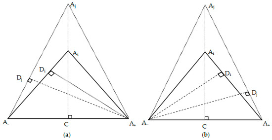
Figure 1. Schematic diagram of bidirectional projection method. (a) Schematic diagram of CBPM; (b) Schematic diagram of IBPM.

As shown in Figure 1a, ${Prj}_{A_{-}{A}_{+}}(A_i{A}_{+})={Prj}_{A_{-}{A}_{+}}(A_j{A}_{+})$, so if only the unidirectional projections of $A_i$ and $A_j$ onto $A_{-}{A}_{+}$ are considered, respectively, alternatives $A_i,A_j$ cannot be distinguished in terms of superiority. However, if we further consider the distances between $A_i$ and $A_{+}$ or $A_j$ and $A_{+}$, or the angles formed between $A_i{A}_{-}$ and $A_{-}{A}_{+}$ or $A_j{A}_{-}$ and $A_{-}{A}_{+}$, alternative $A_i$ is clearly superior to alternative $A_j$.

On the other hand, Equation (10) can be employed to evaluate the advantages and disadvantages of alternative $A_i,A_j$. As shown in Figure 1a, since $\angle A_{+}{A}_{-}{A}_i<\angle A_{+}{A}_{-}{A}_j$, $‖A_{-}{D}_i‖=‖A_{+}{A}_{-}‖\cos \angle A_{+}{A}_{-}{A}_i$, $‖A_{-}{D}_j‖=‖A_{+}{A}_{-}‖\cos \angle A_{+}{A}_{-}{A}_j$, it follows that $‖A_{-}{D}_j‖<‖A_{-}{D}_i‖$, namely

$${Prj}_{A_j{A}_{+}}(A_{-}{A}_{+})<{Prj}_{A_i{A}_{+}}(A_{-}{A}_{+})$$

(12)

According to Equation (10), we obtain

$$\left\{\begin{array}{c}{\lambda }_i={\displaystyle \frac{Pr{j}_{A_{-}{A}_{+}}(A_i{A}_{-})}{Pr{j}_{A_{-}{A}_{+}}(A_i{A}_{-})+Pr{j}_{A_{i}A+}(A_{-}{A}_{+})}}\\ {\lambda }_j={\displaystyle \frac{Pr{j}_{A_{-}{A}_{+}}(A_j{A}_{-})}{Pr{j}_{A_{-}{A}_{+}}(A_j{A}_{-})+Pr{j}_{A_{j}A+}(A_{-}{A}_{+})}}\end{array}\right..$$

(13)

From Equations (11)–(13), it can be readily derived that ${\lambda }_j>{\lambda }_i$. This implies that alternative $A_j$ is superior to alternative $A_i$, which contradicts the aforementioned assertion.

The reason for this inconsistency lies in the fact that the formulas for the closeness degree fundamentally originate from the TOPSIS method. In TOPSIS-based decision making, alternatives $A_i$ are ranked according to the relative closeness degree ${\mu }_i=S_i^{-}/(S_i^{-}+S_i^{+})$, where $S_i^{+}$ and $S_i^{-}$ represent the distances of alternative $A_i$ to the PIS and NIS, respectively. A larger ${\mu }_i$ indicates a better alternative. In this structure of relative closeness, $S_i^{+}$ plays a dominant role in determining the value of ${\mu }_i$. A larger $S_i^{+}$ leads to a larger ${\mu }_i$ and thus a better alternative, whereas $S_i^{-}$ has a comparatively lesser influence on ${\mu }_i$. In the BP method, $S_i^{+}$ is characterized by ${Prj}_{A_{-}{A}_{+}}(A_i{A}_{+})$. Therefore, when constructing the relative closeness degree for the BP method, it is also essential to emphasize the dominant role of ${Prj}_{A_{-}{A}_{+}}(A_i{A}_{+})$.

3.2.3. Definition of a New Closeness Degree

Based on Section 3.2.2, a new definition of closeness degree for the BP method is proposed as follows:

Definition 9.

The closeness coefficient of the BP method is defined as

$${\lambda *}_i={\displaystyle \frac{Pr{j}_{A_i{A}_{-}}(A_{-}{A}_{+})}{Pr{j}_{A_i{A}_{-}}(A_{-}{A}_{+})+Pr{j}_{A_{-}A+}(A_i{A}_{+})},}$$

(14)

where a larger value of ${\lambda *}_i$ indicates that alternative $A_i$ is better, and vice versa.

The rationality of the IBPM can also be verified from Figure 1b. As shown in Figure 1b, $‖A_{+}{D}_j‖<‖A_{+}{D}_i‖$, which implies ${Prj}_{A_j{A}_{+}}(A_{-}{A}_{+})<{Prj}_{A_i{A}_{+}}(A_{-}{A}_{+})$. Furthermore, since $A_i{A}_j\perp A_{-}{A}_{+}$, we have ${Prj}_{A_{-}{A}_{+}}(A_i{A}_{+})={Prj}_{A_{-}{A}_{+}}(A_j{A}_{+})$. Substituting these into Equation (14), it is easily deduced that ${\lambda *}_j<{\lambda *}_i$. This indicates that $A_i$ is superior to $A_j$, which aligns with the analytical conclusion regarding alternative ranking discussed previously. This demonstrates that ranking alternatives using the new closeness coefficient ${\lambda *}_i$ is more reasonable.

3.3. Steps of the BP Grey Target GDMM Under TPIGN

This section first presents the normalization method for the original decision matrix with TPIGN, as well as a method for determining index weights based on TPIGN. Subsequently, the definitions of the positive BED and negative BED after aggregating GDM information, along with the definitions of the closeness degree, are established. Finally, the specific steps of the BP grey target GDMM under TPIGN are summarized.

3.3.1. Normalization of Decision Matrix

Let ${\overline{r}}_j^{*}=\underset{1\le i\le n}{\max }\left\{{\overline{r}}_{ij}\right\},\hspace{1em}{\underset{¯}{r}}_j^{\nabla }=\underset{1\le i\le n}{\min }\left\{{\underset{¯}{r}}_{ij}\right\}(j=1,2,\cdots ,m)$. For benefit criteria:

$${\underset{¯}{x}}_{ij}={\displaystyle \frac{{({\underset{¯}{r}}_{ij}-{\underset{¯}{r}}_j^{\nabla })}^{1/2}}{{({\overline{r}}_j^{*}-{\underset{¯}{r}}_j^{\nabla })}^{1/2}}},{\tilde{x}}_{ij}={\displaystyle \frac{{({\tilde{r}}_{ij}-{\underset{¯}{r}}_j^{\nabla })}^{1/2}}{{({\overline{r}}_j^{*}-{\underset{¯}{r}}_j^{\nabla })}^{1/2}}},{\overline{x}}_{ij}={\displaystyle \frac{{({\overline{r}}_{ij}-{\underset{¯}{r}}_j^{\nabla })}^{1/2}}{{({\overline{r}}_j^{*}-{\underset{¯}{r}}_j^{\nabla })}^{1/2}}}.$$

(15)

For cost criteria:

$${\underset{¯}{x}}_{ij}={\displaystyle \frac{{({\overline{r}}_j^{*}-{\overline{r}}_{ij})}^{1/2}}{{({\overline{r}}_j^{*}-{\underset{¯}{r}}_j^{\nabla })}^{1/2}}},{\tilde{x}}_{ij}={\displaystyle \frac{{({\overline{r}}_j^{*}-{\tilde{r}}_{ij})}^{1/2}}{{({\overline{r}}_j^{*}-{\underset{¯}{r}}_j^{\nabla })}^{1/2}}},{\overline{x}}_{ij}={\displaystyle \frac{{({\overline{r}}_j^{*}-{\underset{¯}{r}}_{ij})}^{1/2}}{{({\overline{r}}_j^{*}-{\underset{¯}{r}}_j^{\nabla })}^{1/2}}}$$

(16)

after normalizing the original decision matrix, a TPIGN normalized decision matrix ${\widehat{R}}^L={(x_{ij}(\otimes ))}_{n\times m}$, $i=1,2,\cdots ,n,j=1,2,\cdots m$, where $L$ denotes the expert number, can be obtained.

3.3.2. Method for Determining Criteria Weights Based on TPIGN

In practical decision-making processes, due to the complexity and uncertainty in experts’ descriptions of criteria importance, evaluative information is often provided in the form of INs. When a IN is used to represent a parameter, it is assumed that all values within the entire interval are equally probable, which may lead to significant deviations from the experts’ true intentions. Therefore, this section proposes a new method for determining criteria weights based on TPIGN.

Let expert $S_i$ $(i=1,2,\cdots ,n)$ give scores $[{\underset{¯}{s}}_{ij},{\tilde{s}}_{ij},{\overline{s}}_{ij}]$ for criteria $j(j=1,2,\cdots m)$ on a percentage scale. Normalize the TPIGN $[{\underset{¯}{w}}_{ij},{\tilde{w}}_{ij},{\overline{w}}_{ij}]$ of the weights using the following formula,

$${\underset{¯}{w}}_{ij}={\underset{¯}{s}}_{ij}/{\displaystyle \sum _{j=1}^m{\underset{¯}{s}}_{ij}},\hspace{1em}{\tilde{w}}_{ij}={\tilde{s}}_{ij}/{\displaystyle \sum _{j=1}^m{\underset{¯}{s}}_{ij}},\hspace{1em}{\overline{w}}_{ij}={\overline{s}}_{ij}/{\displaystyle \sum _{j=1}^m{\underset{¯}{s}}_{ij}}.$$

(17)

where ${\tilde{w}}_{ij}$ is the center of gravity of $[{\underset{¯}{w}}_{ij},{\tilde{w}}_{ij},{\overline{w}}_{ij}]$, $i=1,2,\cdots ,n,j=1,2,\cdots m$.

Let $d_j^{\pm }={\overline{w}}_j^{+}-{\underset{¯}{w}}_j^{-}$, $j=1,2,\cdots m$ be the maximum measure of the upper and lower bounds of the weight estimate for criteria $j(j=1,2,\cdots m)$, where ${\underset{¯}{w}}_j^{-}=\min \{{\underset{¯}{w}}_{1j},{\underset{¯}{w}}_{2j},\cdots {\underset{¯}{w}}_{nj}\}$, ${\overline{w}}_j^{+}=\max \{{\overline{w}}_{1j},{\overline{w}}_{2j},\cdots {\overline{w}}_{nj}\}$, $j(j=1,2,\cdots m)$.

Let the deviation degree of the weight determination provided by expert $s_i$ $(i=1,2,\cdots ,n)$ be $h_{si}$,

$$h_{si}={\displaystyle \frac{w_{ij}^{*}-{\tilde{w}}_{ij}}{d_j^{\pm }}}={\displaystyle \frac{w_{ij}^{*}-{\tilde{w}}_{ij}}{{\overline{w}}_j^{+}-{\underset{¯}{w}}_j^{-}}}={\displaystyle \frac{{\displaystyle \sum _{j=1}^m(w_{ij}^{*}-{\tilde{w}}_{ij})}}{{\displaystyle \sum _{j=1}^m({\overline{w}}_j^{+}-{\underset{¯}{w}}_j^{-})}}}={\displaystyle \frac{{\displaystyle \sum _{j=1}^m{w}_{ij}^{*}}-{\displaystyle \sum _{j=1}^m{\tilde{w}}_{ij}}}{{\displaystyle \sum _{j=1}^m({\overline{w}}_j^{+}-{\underset{¯}{w}}_j^{-})}}}={\displaystyle \frac{1-{\displaystyle \sum _{j=1}^m{\tilde{w}}_{ij}}}{{\displaystyle \sum _{j=1}^m({\overline{w}}_j^{+}-{\underset{¯}{w}}_j^{-})}}}$$

(18)

Here, $w_{ij}^{*}$ represents the true weight of criteria $j(j=1,2,\cdots m)$ as perceived by expert $S_i$, and $h_{si}$ denotes the ratio between the weight error of criteria $j$ given by expert $S_i$ and $d_j^{\pm }$. For each participating expert, it can be assumed that $h_{si}$ is consistent for every evaluation criteria $j(j=1,2,\cdots m)$. Therefore, the estimated value for the weight of $w_j^{*}$ $(j=1,2,\cdots m)$ criteria $j$ is given by:

$${\widehat{w}}_j^{*}=h_s({\overline{w}}_j^{+}-{\underset{¯}{w}}_j^{-})+{\tilde{w}}_j.$$

(19)

where ${\tilde{w}}_j$ is an aggregation of ${\tilde{w}}_{ij}$ $(i=1,2,\cdots n,j=1,2,\cdots m)$ and $h_s$ is an aggregation of $h_{si}$ across all participating experts. It can be easily shown that ${\displaystyle \sum _{j=1}^m{\widehat{w}}_j^{*}}=1$.

For simplicity, the following formulas can be used for aggregation:

$$h_s={\displaystyle \frac{1}{n}}{\displaystyle \sum _{i=1}^n{h}_{si}}, {\tilde{w}}_j={\displaystyle \frac{1}{n}}{\displaystyle \sum _{i=1}^n{\tilde{w}}_{ij}},j=1,2,\cdots m.$$

(20)

Substituting these into Equation (19), the estimated values ${\widehat{w}}_j^{*}$ of the aggregated weights for each criteria can be obtained.

3.3.3. Definition of Positive and Negative BED After Aggregation of GDM Information

Let $\overline{R}={({\mathcal{l}}_{ij}(\otimes ))}_{s\times t}$ be the decision matrix obtained after aggregating GDM information. Denote the positive and negative BE vectors as ${\mathcal{l}}_{Mj}(\otimes )$ and ${\mathcal{l}}_{mj}(\otimes )$, respectively, where

$$\begin{array}{c}{\mathcal{l}}_{Mj}(\otimes )=\underset{i}{\max }({\mathcal{l}}_{ij}(\otimes )),i=1,2,\cdots s,j=1,2,\cdots t.\\ {\mathcal{l}}_{mj}(\otimes )=\underset{i}{\min }({\mathcal{l}}_{ij}(\otimes )),i=1,2,\cdots s,j=1,2,\cdots t.\end{array}$$

(21)

Then

$$\left\{\begin{array}{c}{\epsilon }_i^{+}={[{\displaystyle \sum _{j=1}^t{w}_j{({\mathcal{l}}_{ij}-{\mathcal{l}}_{Mj})}^2}]}^{1/2}\\ {\epsilon }_i^{-}={[{\displaystyle \sum _{j=1}^t{w}_j{({\mathcal{l}}_{ij}-{\mathcal{l}}_{mj})}^2}]}^{1/2}\\ {\epsilon }^{\pm }={[{\displaystyle \sum _{j=1}^t{w}_j{({\mathcal{l}}_{Mj}-{\mathcal{l}}_{mj})}^2}]}^{1/2}\end{array}\right.,$$

(22)

Here, ${\epsilon }_i^{+},{\epsilon }_i^{-}$, $i=1,2,\cdots ,n$, are respectively referred to as the positive BED and the negative BED of alternative $A_i$, $i=1,2,\cdots ,s$, and ${\epsilon }^{\pm }$ is the positive–negative BED in this evaluation process, where $w_j, j=1,2,\cdots t$ are the weights of the evaluation criteria.

3.3.4. Determination of Closeness Degree

According to Section 3.2.2 and Definition 9, the closeness degree for BP under TPIGN can be obtained as follows:

$${\lambda *}_i={\displaystyle \frac{Pr{j}_{{\epsilon }_i^{-}}({\epsilon }^{\pm })}{Pr{j}_{{\epsilon }_i^{-}}({\epsilon }^{\pm })+Pr{j}_{{\epsilon }^{\pm }}({\epsilon }_i^{+})}},i=1,2,\cdots ,s$$

(23)

where ${Prj}_{{\epsilon }_i^{-}}({\epsilon }^{\pm })$ is the projection of ${\epsilon }^{\pm }$ onto ${\epsilon }_i^{-}$, and $Pr{j}_{{\epsilon }^{\pm }}({\epsilon }_i^{+})$ is the projection of ${\epsilon }_i^{+}$ onto ${\epsilon }^{\pm }$, namely

$$\begin{gathered} Pr{j}_{{\epsilon }_i^{-}}({\epsilon }^{\pm })={\epsilon }^{\pm }\cdot \cos ({\epsilon }^{\pm },{\epsilon }_i^{-})={\displaystyle \frac{{({\epsilon }^{\pm })}^2+{({\epsilon }_i^{-})}^2-{({\epsilon }_i^{+})}^2}{2{\epsilon }_i^{-}}},i=1,2,\cdots ,s, \\ Pr{j}_{{\epsilon }^{\pm }}({\epsilon }_i^{+})={\epsilon }_i^{+}\cdot \cos ({\epsilon }^{\pm },{\epsilon }_i^{+})={\displaystyle \frac{{({\epsilon }^{\pm })}^2+{({\epsilon }_i^{+})}^2-{({\epsilon }_i^{-})}^2}{2{\epsilon }^{\pm }}},i=1,2,\cdots ,s. \end{gathered}$$

(24)

3.3.5. BP Grey Target GDMM Steps Based on TPIGN

As mentioned earlier, this section presents a novel grey target GDMM based on TPGIN. The specific steps are as follows:

Step 1: The expert panel scores the importance degree of each criterion on a percentage scale, with scores given as TPIGNs. Determine the weight $w_j, j=1,2,\cdots m$ for each criterion according to Section 3.3.2 (see lines 1 to 4 in Algorithm 2).

Step 2: Every expert provides a TPIGN effect measure matrix for the alternative set with respect to the criterion set. Normalize the matrix using the method described in Section 3.3.1 to obtain the normalized TPIGN decision matrix ${\widehat{R}}^L={(x_{ij}(\otimes ))}_{s\times m}$, where $L,L=1,2,\cdots ,K$ denotes the expert’s identification number (see lines 5 to 8 in Algorithm 2).

Step 3: Based on Section 3.1.3, the aggregated decision matrix $\overline{R}={({\mathcal{l}}_{ij}(\otimes ))}_{s\times m}$ can be obtained; then, calculate the positive and negative BE, the positive BED ${\epsilon }_i^{+},i=1,2,\cdots ,s$, the negative BED ${\epsilon }_i^{-},i=1,2,\cdots ,s$, and the positive–negative BED ${\epsilon }^{\pm }$ for each alternative using Equation (22) (see lines 9 to 16 in Algorithm 2).

Step 4: Rank the alternatives by calculating the closeness degree for each alternative according to Equation (23) (see lines 17 to 18 in Algorithm 2).

To further illustrate the above steps, the algorithm of grey target GDM based on the TPIGN and IBPM is presented in Algorithm 2.

Algorithm 2. The algorithm of grey target GDM based on TPIGN and IBPM

Input: Set of experts $E=\{1,2,\cdots ,K\}$  Set of criteria $C=\{1,2,\cdots ,m\}$  Set of alternatives $A=\{1,2,\cdots ,s\}$  Importance score $I_{k,j}$ (in TPIGN form) given by expert $k$ for criterion $j$    Effect measure $E_{k,i,j}$ (in TPIGN form) given by expert $k$ for alternative $i$ under criterion $j$  Output: Ranking of alternatives (descending order of preference)

//Determine criterion weights 1 For each $j\in C$ do 2  Compute weight ${\omega }_j$ from the importance scores of all experts using the method described in Section 3.3.2 3 End 4 Obtain weight vector $W=({\omega }_1,{\omega }_2,\cdots ,{\omega }_m)$  //Normalize each expert’s decision matrix 5 For each $k\in E$ do 6  Construct the raw matrix $R_k={[E_{k,i,j}]}_{s\times m}$  7  Normalize $R_k$ using the method in Section 3.3.1 to obtain the normalized matrix ${\widehat{R}}^k={[x_{ij}{(\otimes )}_k]}_{s\times m}$  8 End //Aggregate expert matrices and compute positive/negative BED 9 Aggregate all ${\widehat{R}}^k$ to obtain $\overline{R}={[{\mathcal{l}}_{ij}(\otimes )]}_{s\times m}$  10 For each $j\in C$ do 11 Compute the positive benchmark value $B{E}_j^{+}$ and negative benchmark value $B{E}_j^{-}$  12 End 13 For each $i\in A$ do 14  Compute the positive BED ${\epsilon }_i^{+}$, the negative BED ${\epsilon }_i^{-}$, and the positive–negative BED ${\epsilon }_i^{\pm }$ for alternatives using Equation (22) 15 Calculate the closeness degree $C_i$ from ${\epsilon }_i^{+}$ ${\epsilon }_i^{-}$ and ${\epsilon }_i^{\pm }$ using Equation (23) 16 End //Rank alternatives 17 Sort alternatives in descending order of $C_i$  18 Return the ranked list of alternatives.

4. Example Verification and Result Analysis

In this section, the algorithm proposed above is applied to two application scenarios, namely carrier-based aircraft selection and PQ assessment, to validate the rationality and scientific rigor of the proposed algorithm. All data were calculated using MATLAB R2019a software. The computations were performed on a Lenovo Yangtian S5430-00 computer equipped with an Intel(R) Core(TM) i5-10210U CPU Produced by Lenovo, a company from China, running at a base frequency of 1.60 GHz and 8.00 GB of memory.

4.1. Application in Carrier-Based Aircraft Selection

As one of the most crucial offensive means of naval vessels, the selection of aircraft types determines the combat capability of the ship. This section employs an example of carrier-based aircraft selection to verify the scientific validity and effectiveness of the group decision-making method proposed in this paper. This example also serves as a classic case for validating decision-making methods using TPIGN and has been widely adopted in numerous literature sources [7,8]. In the following, the IBPM, the CBPM, and the relative bullseye distance method (RBEDM) will be applied to the carrier-based aircraft selection example.

4.1.1. Example Validation Background

The primary parameters for carrier-based aircraft selection include six criteria: maximum speed (C1), over-sea free range (C2), maximum net payload (C3), acquisition cost (C4), reliability (C5), and maneuverability (C6). There are four available aircraft models to choose from, forming the set of alternatives. This case is used to validate the effectiveness of the improved bidirectional projection grey target group decision-making method.

An expert panel comprising seven specialists in military equipment was organized to provide TPIGN evaluations for the corresponding criteria of the four carrier-based aircraft models. Among them, five experts also assigned TPIGN scores to indicate the importance of each criterion.

4.1.2. Experimental Procedure and Results

Step 1: Determine the weights of each criterion. Five experts provide TPIGN scores for the importance of the six evaluation criteria. According to Section 3.3.2, the weight vector for the six criteria is calculated as:

$$w=[0.1410 0.1405 0.1657 0.1771 0.1905 0.1853]$$

Step 2: Obtain the normalized decision matrix of expert evaluations.

Seven experts $E_i,i=1,2,\cdots ,7.$ are organized to provide TPIGN evaluations for the six criteria regarding the four types of carrier-based aircraft. Normalization is performed following the procedure described in Section 3.3.1.

Step 3: Aggregate the group decision-making information and calculate the positive and negative BE, the positive BED, the negative BED, and the positive–negative BED for each alternative.

First, using MATLAB software and following Equation (9) in Section 3.1.3 (with the Orness measure uniformly set to 0.6), the weight coefficients of the ITPIGN-WA operator are solved as [0.2071, 0.1857, 0.1643, 0.1429, 0.1214, 0.1000, 0.0786]. After completing the information aggregation, the group decision-making matrix is obtained.

$$\overline{R}={({\mathcal{l}}_{ij}(\otimes ))}_{4\times 6}=\left[\begin{array}{cccccc}0.7558& 0.7440& 0.9592& 0.7959& 0.8390& 0.7798\\ 0.7939& 0.8945& 0.6881& 0.5446& 0.4053& 0.5419\\ 0.8911& 0.7770& 0.8539& 0.7317& 0.7813& 0.8964\\ 0.7132& 0.7032& 0.8531& 0.6435& 0.5806& 0.5230\end{array}\right]$$

(25)

The positive and negative BE vectors ${\mathcal{l}}_{Mj}(\otimes ),{\mathcal{l}}_{mj}(\otimes )$ of the group decision matrix are:

$$\left\{\begin{array}{c}{\mathcal{l}}_{Mj}(\otimes )=[0.8911,0.8945,0.9592,0.7959,0.8390,0.8964]\\ {\mathcal{l}}_{mj}(\otimes )=[0.7132,0.7032,0.688,0.5446,0.4053,0.5230]\end{array}\right.$$

(26)

From Equation (23), the positive–negative BED ${\epsilon }^{\pm }=0.3076$. The positive BED ${\epsilon }_i^{+}$, the negative BED ${\epsilon }_i^{-}$ are obtained as:

$${\epsilon }_i^{+}=[0.0910, 0.2895, 0.0717, 0.2327],{\epsilon }_i^{-}=[0.2681,0.0783,0.2622,0.1100]$$

Step 4: Calculate the ranking of alternatives under different decision-making methods.

Using the RBEDM as a reference, the CBPM and the IBPM are applied to calculate the rankings of the four candidate carrier-based aircraft types. The specific results are shown in Table 4 below:

Table 4. Calculation results and ranking of carrier-based aircraft types by different methods.

Method	${\mathit{S}}_1$	${\mathit{S}}_2$	${\mathit{S}}_3$	${\mathit{S}}_4$	Ranking Result
RBEDM	0.7717	0.5152	0.8109	0.5694	$S_3\succ S_1\succ S_4\succ S_2$
CBPM	0.6950	0.0085	0.5856	0.0781	$S_1\succ S_3\succ S_4\succ S_2$
IBPM	0.9716	0.1299	0.9728	0.5367	$S_3\succ S_1\succ S_4\succ S_2$

As can be seen from Table 4, after the group information aggregation is completed, the ranking results of carrier-based aircraft types calculated using the IBPM and the RBEDM are consistent, both being $S_1\succ S_3\succ S_4\succ S_2$. This is consistent with the conclusions in the literature and aligns with the actual evaluation results. Moreover, Table 4 also indicates that the calculation result using the CBPM is $S_3\succ S_1\succ S_2\succ S_4$, which differs from the ranking results obtained with the IBPM and RBEDM. In particular, the rankings of carrier-based aircraft $S_2$ and $S_4$ are exactly reversed. This ranking confirms that IBPM prioritizes forward projection, which aligns with the practical requirement of ‘performance-first’ in carrier-based aircraft selection.

4.2. Application of Comprehensive Power Quality (PQ) Assessment

Comprehensive PQ assessment is a process that involves evaluating various PQ criteria based on actual measurements of electrical operating parameters in power systems or simulation modeling to obtain foundational data. With the continuous development of new-type power systems, conducting scientific and reasonable quantitative assessments of PQ has become increasingly crucial [27]. In this section, test data from the literature will be referenced to conduct a comprehensive PQ assessment across four quarters [28].

4.2.1. Sample Validation Background

Taking into full consideration the correlations among PQ criteria, six metrics are selected to construct the evaluation criterion system: voltage deviation ($C_1$), three-phase voltage unbalance ($C_2$), voltage harmonic ($C_3$), voltage fluctuation ($C_4$), voltage interharmonic ($C_5$) and frequency deviation ($C_6$). To ensure the comparability of PQ data across different quarters in the literature, the data from the first 364 days in the literature are sequentially divided into 28 matrices, each of size $13\times 6$. Every set of 7 matrices corresponds to the PQ data of one quarter. From each matrix, the minimum, average, and maximum values of each column are selected to form a TPIGN, which can be regarded as an evaluation value of a specific PQ criteria for a given period (13 days) within a quarter (as shown in Table A1 in Appendix A).

4.2.2. Experimental Procedure and Results

To ensure the consistency of the computational results, the weights for PQ indices were directly adopted from the findings in Caihua et al. [28].

$$w=[0.0239 0.5555 0.2304 0.0575 0.1120 0.0207]$$

The group decision matrix is obtained after the information is fully aggregated, as follows:

$$\overline{R}={({\mathcal{l}}_{ij}(\otimes ))}_{4\times 6}=\left[\begin{array}{cccccc}0.6438& 0.5007& 0.6375& 0.9624& 0.6825& 0.6199\\ 0.5665& 0.7509& 0.4864& 0.6469& 0.5993& 0.8121\\ 0.3683& 0.7796& 0.2323& 0.8767& 0.7569& 0.5704\\ 0.4062& 0.7609& 0.6745& 0.9382& 0.7182& 0.4062\end{array}\right]$$

(27)

The positive and negative BE vectors are, respectively,

$$\left\{\begin{array}{c}{\mathcal{l}}_{Mj}(\otimes )=[0.6438,0.7796,0.6745,0.9624,0.7569,0.8121]\\ {\mathcal{l}}_{mj}(\otimes )=[0.3683,0.5007,0.2323,0.6469,0.5993,0.4062]\end{array}\right.$$

(28)

and

$$\begin{array}{c}{\epsilon }_i^{\pm }=0.3193\\ {\epsilon }_i^{-}=[0.2119, 0.1314, 0.2202, 0.0718]\\ {\epsilon }_i^{+}=[0.2170, 0.2323, 0.2277, 0.2986]\end{array}$$

The RBEDM, CBPM and IBPM were applied to calculate PQ for four quarters, with the specific ranking results presented in Table 5.

Table 5. PQ ranking by quarter.

Method	${\mathit{S}}_1$	${\mathit{S}}_2$	${\mathit{S}}_3$	${\mathit{S}}_4$	Ranking Result
RBEDM	0.6011	0.7085	0.5919	0.8164	$S_4\succ S_2\succ S_1\succ S_3$
CBPM	0.3241	0.4333	0.3317	0.8439	$S_4\succ S_2\succ S_3\succ S_1$
IBPM	0.7023	0.8951	0.6823	0.9919	$S_4\succ S_2\succ S_1\succ S_3$

As can be seen from Table 5, the ranking results of PQ for the four quarters calculated using the IBPM and the RBEDM are consistent, both being $S_4\succ S_2\succ S_1\succ S_3$. Furthermore, Table 5 shows that the calculation result obtained using the CBPM is $S_4\succ S_2\succ S_1\succ S_3$, which differs from the ranking results derived from the IBPM and the RBEDM. Specifically, the rankings of PQ in the third quarter and the first quarter are exactly reversed.

As shown in Table 5, the PQ rankings for the four quarters ($S_1$, $S_2$, $S_3$, $S_4$) obtained by three different methods are compared. The IBPM and the RBEDM yield identical ranking orders: $S_4\succ S_2\succ S_1\succ S_3$. In contrast, the CBPM produces a different sequence: $S_4\succ S_2\succ S_3\succ S_1$. The only discrepancy lies in the relative positions of $S_1$ and $S_3$, which are exactly reversed between the two sets of results.

A closer look at the numerical values reveals that while IBPM generates consistently higher scores than RBEDM (e.g., IBPM: 0.7023 vs. RBEDM: 0.6011 for $S_1$ ), the preservation of the same ranking order across four alternatives underscores the strong consistency between IBPM and the benchmark method. This alignment supports the validity of IBPM as a reliable decision tool. Meanwhile, CBPM not only swaps the order of $S_1$ and $S_3$ but also exhibits relatively low scores for both (0.3241 and 0.3317), suggesting possible distortion in its proximity measures.

The observed ranking reversal is not an isolated case. A similar phenomenon occurs in another numerical example (Table 4), where CBPM again reverses the order of two evaluation objects compared to IBPM and RBEDM. This recurring pattern aligns with the mathematical analysis in Section 3.2.2, which identifies inherent flaws in the traditional BP method’s calculation of closeness degree and consistency coefficient. These flaws lead to biased assessments, particularly when objects have close performance values. The IBPM, by incorporating geometric interpretability, rectifies these deficiencies and ensures that the relative ranking reflects the true spatial relationships with the BE.

Furthermore, the consistent rankings between IBPM and RBEDM across multiple alternatives confirm that the proposed grey target group decision-making model, integrating the ITPIGN-WA operator and the IBPM, achieves both scientific aggregation and decision robustness. The numerical differences between IBPM and RBEDM are attributed to distinct calculation scales, yet the rank preservation demonstrates that IBPM retains the essential decision information without distortion. Overall, the comparative analysis confirms that the IBPM outperforms the CBPM by delivering more reasonable and reliable rankings, especially when handling multi-attribute grey information.

4.3. Analysis of Numerical Experimental Results

From the numerical experiments of carrier-based aircraft selection and comprehensive PQ assessment described above, the following conclusions can be drawn:

(1)

After solving for the weight coefficients of the ITPIGN-WA operator under the Orness measure using Equation (9), the aggregation of group information can be conveniently accomplished.

(2)

Following the aggregation of group information, applying the CBPM and the RBEDM to the examples yields consistent ranking results. These results align with the conclusions provided in the source literature of the examples and match the actual evaluation outcomes, demonstrating the effectiveness and rationality of the grey target GDM model based on the BP method and TPIGN proposed in this paper.

(3)

Furthermore, as indicated in Table 4 and Table 5, in both examples, the calculation results obtained using the CBPM differ from the ranking results derived from the IBPM and the RBEDM. In both cases, the ranking of two evaluation objects is exactly reversed. This reversal is consistent with the mathematical analysis presented in Section 3.2.2, thereby verifying the issues inherent in the CBPM and further confirming that the IBPM is more reasonable and scientific.

4.4. Comparative Analysis of IBPM and Other Grey Decision Frameworks

Traditional grey target decision models often rely on basic whitenization functions as well as the grey relational degree for information aggregation and scheme ranking. While effective for handling uncertainty, these conventional approaches exhibit notable limitations. First, their information processing mechanisms struggle with the complex, multi-faceted uncertainty found in TPIGN, often leading to information loss during conversion. Second, the CBPM possesses inherent mathematical flaws in calculating the closeness degree and consistency coefficient, which can compromise the geometric rationality and reliability of the decision outcomes.

In contrast, the novel decision framework proposed in this study introduces distinct theoretical and methodological advancements. It innovatively establishes a rigorous conversion mechanism between TPIGN and dual CNs, leveraging set pair analysis to fully preserve the intrinsic uncertainty characteristics. Building on this, the proposed ITPIGN-WA operator provides a mathematically robust aggregation method, overcoming the limitations of traditional weighted averaging operators.

Furthermore, this framework fundamentally rectifies the deficiencies of the CBPM. By proposing an IBPM with geometric interpretability, it ensures that the calculation of the consistency coefficient and proximity more accurately reflects the actual spatial relationships between decision targets and the optimal bullseye. This enhancement directly improves the robustness and logical consistency of the ranking process.

Ultimately, by integrating the ITPIGN-WA operator with the IBPM, the new grey target GDMM achieves a superior balance between scientific aggregation and decision robustness. Unlike traditional models that may sacrifice accuracy for simplicity, this proposed framework delivers more reliable and rationally defensible evaluation results, as validated by the empirical study on carrier-based aircraft selection and PQ assessment.

5. Conclusions and Prospects

Based on TPIGN and the BP method, this study constructs a novel grey target group decision-making model (GDMM). The main contributions are:

(1)

A conversion mechanism between TPIGN and dual connection numbers is established. Using set pair possibility theory, an ITPIGN-WA operator with strict mathematical properties is proposed for grey information aggregation.

(2)

Mathematical analysis reveals flaws in traditional BP methods regarding closeness degree and consistency coefficient calculation. An IBPM with geometric interpretability is introduced, enhancing decision reliability.

(3)

Integrating the ITPIGN-WA operator with the refined BP method yields a grey target GDMM that balances aggregation scientific and decision robustness. The empirical study on carrier-based aircraft selection and PQ assessment confirms its superior rationality over conventional methods.

While this study provides a foundation for grey target decision making, several limitations should be acknowledged and addressed in future work. First, the current theoretical framework primarily relies on static information representation and does not yet incorporate multi-granularity fusion, which is crucial for handling heterogeneous data in big-data group decision making. To overcome this, future research can extend the theory by integrating set pair analysis with two-dimensional cloud models to enable multi-granularity grey information fusion. Second, the proposed method lacks dynamic adaptability to evolving decision environments; therefore, subsequent studies may optimize the decision framework using Markov chains and deep reinforcement learning to develop adaptive, real-time decision-making systems. Third, the application scope is limited to specific illustrative cases, which restricts generalizability. Future work should thus apply the approach to broader domains such as smart city risk assessment and public health emergencies, with a focus on multi-agent collaboration and visual decision support systems to enhance practical relevance and scalability.

References

- Kamdar, I.; Liu, S. Evaluating underlying barriers and development pathways for photovoltaic solar energy in China using the grey analytic hierarchy process. Grey Syst. Theory Appl. 2025, 15, 446–461. [Google Scholar] [CrossRef]
- Nawaz, M.; Liu, S.; Xie, N.; Ramzan, B. Evaluation of barriers to artificial intelligence adoption: Grey multi-criteria decision-making. Grey Syst. Theory Appl. 2025, 15, 732–754. [Google Scholar] [CrossRef]
- Liu, S.F.; Lin, Y. Grey Systems Theory and Applications; Springer: Berlin/Heidelberg, Germany, 2010; pp. 197–218. [Google Scholar]
- Song, J.; Dang, Y.G.; Wang, Z.X. New decision model of grey target with both the positive clout and the negative clout. Syst. Eng. Theory Pract. 2010, 30, 1822–1827. [Google Scholar]
- Liu, Z.X.; Liu, S.F.; Jiang, S.Q. Study on the expansion of bidirectional projection grey target decision-making model based on general grey number. Syst. Eng. Theory Pract. 2019, 39, 776–782. [Google Scholar]
- Huang, F.; Zeng, X.; Yan, S.; He, F.; Kuang, H. A seasonal grey model with three parameter-interval grey numbers for forecasting natural gas production. Grey Syst. Theory Appl. 2026, 16, 91–116. [Google Scholar] [CrossRef]
- Bu, G.Z.; Zhang, Y.W. Grey fuzzy comprehensive evaluation method based on interval numbers of three parameters. Syst. Eng. Electron. 2001, 23, 43–45. [Google Scholar]
- Luo, D. Decision-making methods with three-parameter interval grey number. Syst. Eng. Theory Pract. 2009, 29, 124–130. [Google Scholar] [CrossRef]
- Yan, S.L.; Liu, S.F.; Wu, L.F. A group grey target decision making method with three parameter interval grey number based on prospect theory. Control Decis. 2015, 30, 105–109. [Google Scholar]
- Li, C.; Yuan, J. A new multi-attribute decision making method with three-parameter interval grey linguistic variable. Int. J. Fuzzy Syst. 2017, 2, 292–300. [Google Scholar] [CrossRef]
- Wang, X. Gray Multi-Attribute Decision Analysis and Application; Economic Management Press: Beijing, China, 2017; pp. 109–120. [Google Scholar]
- Ye, L.; Zhang, D.X. Multi-attribute Group Grey Target Decision-making Method Based on Three-parameter Interval Grey Number. J. Grey Syst. 2020, 32, 96–109. [Google Scholar]
- Ali, J.; Bashir, Z.; Rashid, T. On distance measure and TOPSIS model for probabilistic interval-valued hesitant fuzzy sets: Application to healthcare facilities in public hospitals. Grey Syst. Theory Appl. 2022, 12, 197–229. [Google Scholar] [CrossRef]
- Yager, R.R. On ordered weighted averaging Aggregation operators in multi-criteria decision making. IEEE Trans. Syst. Man Cybern. B 1988, 18, 183–190. [Google Scholar] [CrossRef]
- Zhou, L.G.; Chen, H.Y.; Liu, J.P. Generalized power aggregation operators and their applications in group decision making. Comput. Ind. Eng. 2012, 62, 989–999. [Google Scholar] [CrossRef]
- Yager, R.R. Induced ordered weighted averaging operators. IEEE Trans. Syst. Man Cybern. B 1999, 29, 141–150. [Google Scholar] [CrossRef] [PubMed]
- Yager, R.R.; Xu, Z.S. The continuous ordered weighted geometric operator and its applications to decision making. Fuzzy Sets Syst. 2006, 157, 1393–1402. [Google Scholar] [CrossRef]
- Xu, Z.S. An overview of methods for determining OWA weights. Int. J. Intell. Syst. 2005, 20, 843–865. [Google Scholar] [CrossRef]
- Wang, X. Information aggregation operators over a continuous three parameters interval argument and their application to decision making. Syst. Eng. Electron. 2008, 30, 1468–1473. [Google Scholar]
- Dong, T.; Wei, Y.; Jin, J.; Zhou, P.; Hu, Y.; Chen, M.; Zhou, Y. Evaluation and Diagnosis of Water Resources Spatial Equilibrium Under the High-Quality Development of Water Conservancy. JAWRA J. Am. Water Resour. Assoc. 2025, 61, e70014. [Google Scholar] [CrossRef]
- Liu, X.; Zhao, K. Application of set pair analysis in the uncertainty intelligent decision making. CAAI Trans. Intell. Syst. 2020, 15, 121–135. [Google Scholar]
- Hu, Y.; Jiang, D.Y.; Li, H. Probabilistic linguistic multi-attribute group decision-making based on bidirectional projection method. Syst. Eng. Electron. 2020, 42, 2052–2059. [Google Scholar]
- Wang, J.; Jing, Z.X. Consistency bidirectional projection decision method within interval hesitation fuzzy information. Stat. Decis. 2019, 35, 59–62. [Google Scholar]
- Zhou, L.; Chen, H.; Wang, X. Induced continuous ordered weighted averaging operators and their applications in interval group decision making. Control Decis. 2010, 25, 179–184. [Google Scholar]
- Ding, X.; Jiang, D.; Yin, Y.; Rao, C. Interval-valued Pythagorean Fuzzy Decision-making Based on the Entropy and Bidirectional Projection. Complex Syst. Complex. Sci. 2025, 22, 88–96. [Google Scholar]
- Wang, S.; Wang, J.; Qiao, Y.; Zhang, R. Modified Bidirectional Projection Technique for Spherical Fuzzy MAGDM and Applications to Demand Evaluation for Public Sports Services for the Elderly in Rural Areas. Int. J. Fuzzy Syst. 2025, 8, 1562–2479. [Google Scholar] [CrossRef]
- Xiao, B.; Zhao, X.; Dong, G. Summary and Prospect of Comprehensive Evaluation Methods of Power Quality. Power Gener. Technol. 2024, 45, 716–733. [Google Scholar]
- Lin, C.; Zhang, Y.; Shao, Z.; Liu, Y. Comprehensive Evaluation of Power Quality on Long-time Scale Based on Fuzzy DEA. High Volt. Eng. 2021, 47, 1751–1758. [Google Scholar]
Disclaimer/Publisher’s Note: The statements, opinions and data contained in all publications are solely those of the individual author(s) and contributor(s) and not of MDPI and/or the editor(s). MDPI and/or the editor(s) disclaim responsibility for any injury to people or property resulting from any ideas, methods, instructions or products referred to in the content. |
© 2026 by the authors. Licensee MDPI, Basel, Switzerland. This article is an open access article distributed under the terms and conditions of the Creative Commons Attribution (CC BY) license.