Abstract
Large, high-quality patient datasets are essential for applications like economic modeling and patient simulation. However, real-world data is often inaccessible or incomplete. Synthetic patient data offers an alternative, and current methods often fail to preserve clinical plausibility, real-world correlations, and logical consistency. This study presents a patient cohort generator designed to produce realistic, statistically valid synthetic datasets. The generator uses predefined probability distributions and Cholesky decomposition to reflect real-world correlations. A dependency matrix handles variable relationships in the right order. Hard limits block unrealistic values, and binary variables are set using percentiles to match expected rates. Validation used two datasets, NHANES (2021–2023) and the Framingham Heart Study, evaluating cohort diversity (general, cardiac, low-dimensional), data sparsity (five correlation scenarios), and model performance (MSE, RMSE, R2, SSE, correlation plots). Results demonstrated strong alignment with real-world data in central tendency, dispersion, and correlation structures. Scenario A (empirical correlations) performed best (R2 = 86.8–99.6%, lowest SSE and MAE). Scenario B (physician-estimated correlations) also performed well, especially in a low-dimensions population (R2 = 80.7%). Scenario E (no correlation) performed worst. Overall, the proposed model provides a scalable, customizable solution for generating synthetic patient cohorts, supporting reliable simulations and research when real-world data is limited. While deep learning approaches have been proposed for this task, they require access to large-scale real datasets and offer limited control over statistical dependencies or clinical logic. Our approach addresses this gap.
1. Introduction
The use of synthetic patient data in medical research is rapidly gaining popularity due to its ability to model large, complex multivariate datasets that replicate actual features while maintaining patient privacy [1]. Large-scale patient datasets play a crucial role in applications such as clinical trial simulations and modeling disease progression, allowing decisionmakers to make evidence-based decisions. The validity of such models relies not only on the mathematical structure of the simulation but also on the realism of the patient cohort being simulated [2]. A highly sophisticated simulation model cannot produce meaningful results if the underlying patient dataset does not accurately reflect real-world patient characteristics [3].
While actual datasets from electronic health records (EHRs), clinical trials, and population studies exist, they are often expensive, difficult to access, incomplete, or lack the essential patient characteristics required for economic modeling. Furthermore, missing data remains a persistent issue, requiring techniques such as imputation or omission, though both approaches carry inherent limitations and risk introducing bias [4,5].
A promising alternative to actual real-world data is the generation of synthetic patient cohorts. However, simple random data generation is insufficient, as it fails to account for interdependencies between variables or enforce biological plausibility. For example, in a realistic dataset, older age should correlate with higher blood pressure, and biologically implausible cases, such as pregnant male patients or pediatric smokers, must be prevented. For a synthetic patient dataset to be useful in modeling, it must replicate not only the marginal distributions of individual characteristics but also the correlations and clinical constraints between multiple variables, ensuring that relationships observed in real-world data are preserved [6].
Most existing methods generate synthetic data without explicit control over inter-variable relationships, which may result in implausible patient profiles. Deep-learning-based approaches often require large, high-quality real datasets for training and struggle to accurately reproduce the complex, high-dimensional relationships present in patient data, especially when data are scarce or privacy-restricted [7]. These models are prone to amplifying biases present in the original data, which can lead to unbalanced or non-representative synthetic cohorts and potentially discriminatory outcomes [7,8]. Furthermore, deep generative models typically operate as “black boxes,” offering limited transparency and interpretability regarding how variable dependencies are established or how clinical logic is enforced [8].
Additionally, many generative models are computationally intensive, requiring significant resources for training and sampling, which can be a barrier in practical healthcare settings [7,9]. Even methods that use statistical resampling or copulas often have difficulty simultaneously preserving marginal distributions and realistic inter-variable correlations, particularly when only summary statistics are available. To address these challenges, a patient cohort generator is needed to create large-scale, realistic synthetic datasets that preserve the underlying statistical properties of the real population. Such a tool must generate patient characteristics that follow real-world statistical distributions while enforcing biological plausibility and preserving meaningful correlations between variables. Although significant research has been conducted on synthetic data generation across various domains including image, text, and tabular data, the complexity, heterogeneity, and incompleteness of real-world patient datasets poses significant challenges in constructing generative models that produce clinically useful synthetic data [10,11,12].
This study aims to develop and validate a patient cohort generator that can create realistic synthetic patient datasets for use for clinical trial simulations and the economic modeling of disease progression. With the goal of enabling researchers to conduct high-quality research without the constraints of data availability limitations or in data-scarce settings, this tool should be able to generate large datasets while preserving the key features of real-world populations. Specifically, it can produce synthetic patient characteristics that follow predefined statistical distributions, enforce correlations between variables to maintain authentic inter-variable relationships, and ensure biological plausibility by applying logical constraints. Additionally, the generator systematically resolves interdependencies among patient characteristics to reflect real-world complexity and coherence in the simulated data. This study introduces a patient cohort generator that addresses the needs of simulation modeling in data-limited environments. It supports explicit parameter definition, dependency resolution, and correlation enforcement. The approach is validated against real-world datasets and compared across varying levels of data availability.
2. Materials and Methods
2.1. Theoretical Background
To accurately impose realistic inter-variable relationships in the simulated cohort, the method applies Cholesky decomposition to a correlation matrix rather than a covariance matrix. This decision is rooted in both practical and methodological necessity. In most real-world settings, especially in the absence of access to raw patient-level data, it is not feasible to derive a full covariance matrix due to the lack of information on variable units and scale. However, correlation coefficients are often reported in the literature or can be reasonably estimated through expert input, making the construction of a correlation matrix far more attainable. To ensure compatibility with this matrix, all variables are first standardized into Z-scores, transforming them to have a mean of zero and a standard deviation of one. This standardization step is essential, as Cholesky decomposition applied to a correlation matrix requires the input variables to be on a common scale, which would not be possible if values were retained in their original units [13,14]. In contrast to methods that infer dependency structures from raw data, our approach assumes that these relationships are known or can be estimated and enforces them explicitly.
Our approach conceptually parallels extensions of the bootstrap method designed for correlated data, where observations are first transformed into uncorrelated forms, resampled, and then transformed back. Such transformation-based strategies preserve underlying dependency structures while allowing flexible resampling or simulation. Similarly, our method ensures that the synthetic cohort retains realistic inter-variable dependencies while enabling data generation under limited or aggregate statistical inputs [15].
The simulation process proceeds in a structured sequence. First, independent random numbers are generated for each parameter–patient combination. These are transformed into sampled values using the inverse cumulative distribution function (CDF) corresponding to each variable’s assigned distribution; special care is taken to ensure that inputs are appropriately clamped to a safe interval. The sampled values are then standardized into Z-scores. Next, to impose the desired correlation structure, the algorithm multiplies the standardized matrix by the Cholesky decomposition of the input correlation matrix. The resulting correlated Z-scores are transformed back into their original scale. Finally, the model applies logical constraints, including hard limits and deterministic formulas, to enforce clinical plausibility. This structured pipeline ensures that the generated data respects user-defined statistical properties and inter-variable relationships.
2.2. Overview
Our patient cohort generator algorithm was developed in Microsoft Excel and implemented using Visual Basic for Applications (VBA). It is designed to produce synthetic patient-level datasets based on user-defined variables, probability distributions, and clinical constraints. All inputs are configured via a structured Excel interface, while the underlying computations and logic are handled by the VBA engine. The following sections outline the key components of the method, including parameter specification, data generation, and constraint handling (Figure 1).
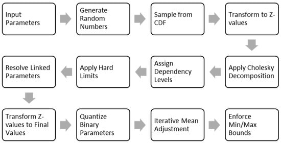
Figure 1.
The flow diagram of the cohort-generation pipeline.
The model’s pipeline begins with the input parameters. For each parameter, the user specifies its type. For continuous variables, the user specifies the probability distribution, as well as the mean, standard deviation, and the minimum and maximum plausible values. For binary variables, only the prevalence is required. The model also allows for a correlation matrix to be defined. Furthermore, equations to define hard limits or linking one parameter to another can be specified. The process then moves to generate random numbers, which are used to sample from CDF by applying the inverse CDF, generating initial raw values for every patient.
To prepare the data for correlation, the initial raw values are standardized into Z-scores, which shifts their distribution to have a mean of zero and a standard deviation of one. This standardization is essential because it brings all variables onto a common scale, a prerequisite for the subsequent correlation step (Cholesky Decomposition). The correlation matrix is then decomposed into a lower triangular matrix, which is then multiplied by the vector of Z-values for each synthetic patient. This transforms the independent data into a set of correlated Z-scores that reflect the complex, real-world relationships between variables.
Before applying hard limits and resolving linked parameters, the model must then evaluate dependency levels, establishing a logical calculation order. Parameters with no dependencies are calculated first (Level 1), followed by those that depend on level 1 parameters only (Level 2), and so on. With the calculation order set, the model can then apply hard limits, which are user-defined rules that prevent clinically implausible scenarios, such as a pediatric patient being recorded as a smoker. Finally, it can resolve linked parameters, calculating their values deterministically based on the already-finalized dependent variables.
The next step is to convert the correlated Z-values to final values back from their original scale. Following this, the model will quantify the binary parameters. The generated values are compared against a quantile of the generated sample that corresponds to the target prevalence of the variable. This ensures that the final proportion of binary outcomes in the synthetic cohort precisely matches the user input.
Due to the slight distortion of mean values of the continuous parameters during the correlation application, as well as clamping the values between the minimum and maximum values, mean adjustment is performed to align the simulated means with user inputs, after which minimum and maximum bounds are enforced to clamp any values that fall outside a plausible range, and this process is repeated until the mean error is sufficiently small.
2.3. Parameter Specification
Users begin by specifying the full set of variables to be simulated. For each variable, the user defines a descriptive name, a code name (for internal reference), and a variable type (continuous, binary or categorical). All parameters are entered through a standardized input sheet within the Excel interface.
For continuous variables, users must specify the mean (), standard deviation (), and minimum and maximum values. These inputs define the expected statistical properties and plausible clinical bounds of the variable. A probability distribution function—such as normal, log-normal, or beta—is selected to determine the underlying distribution used by the patient cohort generator algorithm.
For binary variables, only the mean (interpreted as the probability of positive outcome) is required. Minimum and maximum values default to 0 and 1, respectively. The standard deviation is calculated from the Bernoulli distribution using the following expression:
For categorical variables, list each category in a separate row of the input sheet and assign proportional weights to each category such that the sum equals 1 for every variable group. As with binary variables, the minimum and maximum values default to 0 and 1, and the standard deviation for each category is computed using the same Bernoulli-based formula.
The patient-cohort-generator algorithm also supports the definition of correlations between continuous variables through a correlation matrix. These correlations can be entered manually or imported from a built-in empirical database [16]. The built-in empirical database derives from Wang et al.’s (2022) study of 803,614 individuals, containing 221 physical examination indicators with 7662 documented correlations across healthy and disease states (hypertension, diabetes, etc.) [17].
2.4. Hard Limits and Linked Variables
To ensure both biological plausibility and logical consistency, the patient-cohort-generator algorithm enforces two classes of deterministic logic: hard limits and linked parameters. These mechanisms prevent implausible assignments and preserve coherent relationships among variables.
Hard limits are user-defined logical conditions that restrict the assignment of parameter values based on the values of other variables. These conditions are specified in the input sheet as formula strings using standard logical operators (e.g., AND(), OR(), IF()) and comparison symbols (=, >, <, <>). For example, a constraint for the menopause parameter might be entered as AND(Female = 1, Age > 40), indicating that menopause can only be assigned one if the patient is female and older than 40. During simulation, the algorithm evaluates each patient individually by substituting their specific values into the constraint formula. If the result of the expression is false, the parameter value is automatically set to zero. This ensures that invalid or clinically inconsistent characteristics are not assigned.
Linked parameters are computed deterministically from other variables. If a parameter is marked as linked in the input sheet, its value is calculated using a user-defined expression. These linking formulas use standard arithmetic and logical operations and are resolved only after all dependent variables have been finalized. For example, a cardiovascular risk score might be defined as Age × 0.1 + SBP × 0.2 + Diabetes × 1.5. If a patient is 60 years old with a systolic blood pressure (SBP) of 150 and a diabetes indicator of 1, the expression evaluates to 60 × 0.1 + 150 × 0.2 + 1 × 1.5 = 37.5.
Complex expressions, such as conditional logic (IF(BMI < 18.5, “Underweight”, …)) or nested calculations are also supported. The evaluated result is then stored as the final value for the linked parameter. This method guarantees internal consistency, preserves user-defined relationships between variables, and ensures that derived parameters remain logically aligned with the rest of the dataset. The steps for parsing and evaluating user-defined hard limits and linked equations are discussed in detail in Appendix A.
All parameters and their resolved values are retained in memory throughout the simulation process. This facilitates efficient access, dependency resolution, and the consistent enforcement of both constraints and derivations during cohort generation.
2.5. Generating Random Numbers
After loading all input parameters, the patient-cohort-generator algorithm generates a matrix of independent random numbers drawn from a uniform distribution between 0 and 1. Each element of the matrix corresponds to a specific parameter–patient combination, with the structure defined as follows:
where is the parameter index, and is the patient index. These random values are used to assign values to each parameter across all patients during the simulation process.
The algorithm allows users to specify a fixed random seed. When a seed is defined, it ensures that the same sequence of random numbers is produced in each run, allowing for exact reproducibility during testing or validation.
2.6. Standardized -Values
To enable the application of inter-variable correlation, the patient cohort generator algorithm standardizes all sampled values into Z-scores. This step ensures that all variables are on a common scale, with a mean of zero and a standard deviation of one, which is a necessary condition for applying Cholesky decomposition to a correlation matrix.
The algorithm first uses the generated uniform random number to sample a value from the probability distribution for each parameter. The sampling is performed using the inverse cumulative distribution function (CDF):
where is the inverse CDF for the distribution assigned to parameter , and is the raw sampled value for patient .
Each sampled value is then transformed into a standardized Z-score using the user-defined mean and standard deviation :
This transformation produces a matrix of standardized values that can be used in correlation adjustments. Standardization allows the algorithm to impose the specified correlation structure consistently across variables, regardless of their original scales. The parameter definitions and the distribution-specific details required for inverse CDF sampling are provided in Appendix B.
2.7. Cholesky Decomposition
To ensure realistic interdependencies between patient characteristics—such as the known associations between older age and higher blood pressure or between diabetes, elevated BMI, and cardiovascular risk—the algorithm applies a correlation structure using Cholesky decomposition [14].
The process begins with a user-defined correlation matrix , which is symmetric and positive semi-definite. Its diagonal entries are all 1, and off-diagonal entries are pairwise correlation coefficients . The matrix is decomposed as follows:
where is a lower triangular matrix. In the context of correlation matrices, which are by definition symmetric and positive semidefinite (and under certain conditions, positive definite), this decomposition allows for the efficient simulation or transformation of multivariate normal distributions. The Cholesky decomposition of is computationally efficient and numerically stable, and it guarantees that the resulting transformation preserves the specified correlation structure. Unlike nonlinear latent methods, this linear transformation preserves the exact structure of the specified correlation matrix and can be directly inspected, verified, and updated by the user.
To introduce correlation into the dataset, the algorithm multiplies each patient’s vector of independent standardized normal variables by the matrix :
The result is a vector of correlated Z-scores that reflects the specified relationships among variables. These correlated Z-values are then transformed back to their original scales using the inverse CDFs associated with each parameter, along with their defined means and standard deviations. This step produces the final, correlated parameter values for each synthetic patient.
2.8. Dependency Levels
In the cohort-generation model, the order in which parameters are computed is critical to ensuring both logical consistency and clinical plausibility. This is especially important when the model incorporates user-defined hard limits or linked equations, as these establish explicit dependencies between parameters. For instance, a parameter like menopause cannot be assigned until both age and sex have been resolved. Similarly, the diagnosis of hypertension might rely on a previously computed value such as systolic blood pressure (SBP).
To enforce the proper resolution order, a binary dependency matrix is constructed that encodes the relationships among parameters (Appendix C). Each entry in this matrix is set to one if parameter depends on parameter and zero otherwise. This matrix is assembled by parsing each parameter’s hard constraints and linking formulas to identify references to other variables. The result is an matrix, where is the number of parameters in the model and which fully describes the directed dependency structure of the system.
Once the dependency matrix is defined, the model uses an iterative algorithm to assign a dependency level to each parameter. Parameters that have no dependencies are given Level 1 status and resolved first. Parameters that depend only on those at Level 1 are assigned Level 2. This process continues in sequence, with each parameter assigned the lowest level consistent with its direct and indirect dependencies. The algorithm proceeds until all parameters are ranked. In principle, a parameter could have a dependency level equal to the total number of parameters, depending on the structure of the system. If the algorithm encounters a circular dependency—where two or more parameters form a closed loop of mutual dependence—it halts execution and raises an error.
With dependency levels assigned, parameters are evaluated sequentially, beginning with those at Level 1 and progressing onward. For example, if age and sex are identified as Level 1 variables, they are computed before SBP, which depends on age and might be placed at Level 2. Hypertension, which may depend on SBP, would then be computed at Level 3. This ordering guarantees that each parameter is resolved only after all the variables it relies on have been assigned valid values.
After resolving the dependency-resolution process is complete, each parameter’s final value is calculated by transforming the correlated Z-score using the following formula:
where is the mean, is the standard deviation, and is the Cholesky-adjusted Z-value for the patient . This transformation reintroduces the parameter’s original scale while preserving the intended correlation structure.
2.9. Resolving Binary Variables
Binary parameters require careful treatment to ensure logical consistency and accurate prevalence within the simulated dataset. Although Monte Carlo simulations often rely on the Beta distribution to model bounded variables, this choice is unsuitable for truly binary outcomes. The Beta distribution performs poorly when the expected proportion is near 0 or 1 or exactly 0.5. In these cases, the distribution becomes sharply peaked or fails to support equal partitioning between the two binary states. This makes it an unreliable basis for binary simulation.
The issue becomes more pronounced when correlation is imposed using Cholesky decomposition. If binary values are first sampled from a continuous distribution such as Beta and then transformed to introduce correlation, the resulting values often extend beyond the [0, 1] bounds. These violations must be corrected—typically by clamping—which distorts the prevalence and introduces bias.
To avoid these problems, the patient-generator algorithm simulates binary variables using a thresholding approach applied to correlated standard normal values. During simulation, each binary parameter is treated as continuous and assigned a standard normal value as part of the Cholesky-adjusted correlation step. After correlation is imposed, the algorithm converts these values to binary outcomes based on the desired prevalence .
The values for a specific binary parameter are sorted in ascending order. For a given target prevalence μ (e.g., 62%), the threshold is determined as the value at the quantile of the sorted list:
In the case of 1000 patients and μ = 0.62, this corresponds to the value ranked 380th in the sorted list (i.e., the 38th percentile). This threshold is used to binarize the variable: all values above or equal to the threshold are assigned a value of 1 (true), and all values below are assigned 0 (false). This method guarantees that the proportion of ones in the simulated dataset exactly matches the input prevalence, regardless of the applied correlation structure. Moreover, because the binary conversion is applied after correlation imposition, it avoids the distortions and boundary violations commonly encountered when trying to impose a correlation on binary variables directly using continuous distributions like the Beta. We validated this approach across a wide range of prevalence values—ranging from approximately 12% to 99%—using multiple binary parameters in the Framingham dataset. In all cases, the generated proportions matched the target values precisely, confirming the reliability and accuracy of the method.
2.10. Adjustments
The patient-generator algorithm includes a post-processing step to correct for small deviations between simulated and target means. These discrepancies can arise due to transformations, correlation adjustments, or rounding effects. To ensure that the simulated dataset remains aligned with user-defined specifications, the algorithm applies an iterative mean correction procedure.
This process applies only to non-binary and non-linked parameters. At each iteration, the model calculates an adjustment factor as the difference between the target mean and the current mean of the simulated values :
This difference is then uniformly added to all values of the parameter across the patient cohort:
After each adjustment, the algorithm enforces user-specified minimum and maximum bounds. Any value that falls outside the valid range is clamped back to the nearest allowable limit. This constraint ensures biological plausibility and prevents outcomes such as negative ages or implausible clinical measurements.
The process is repeated iteratively, recalculating after each adjustment, until the mean error is sufficiently small:
To avoid infinite loops, a maximum of 100 iterations is permitted. This mean correction method ensures that simulated values closely reflect user-defined distributions while maintaining all logical and clinical constraints. It enhances the statistical robustness of the patient-generator algorithm without compromising data integrity.
To evaluate the convergence behavior of the iterative mean correction step, we ran 20 independent simulations using the Framingham dataset with different random seeds, yielding a total of 398 convergence events across continuous parameters. The results demonstrated rapid and consistent convergence: 70% of parameters reached the target mean within a single iteration, 28% within two iterations, and 2% within three iterations. No parameter required more than three iterations, with the mean number of 1.33 iterations. These findings indicate that the initially generated values closely approximate the target means in the majority of cases and that the adjustment algorithm is both computationally efficient and highly effective in fine-tuning the output to meet user-defined specifications.
2.11. Validation Apparatus
The performance of the patient-generator algorithm was evaluated using a structured validation framework designed to test accuracy, generalizability, and robustness. The validation plan tests the generator’s ability to reproduce synthetic cohorts that maintain clinical logic and perform reliably under diverse and constrained input conditions.
The validation strategy entailed a two-step simulation exercise. First, real-world datasets, NHANES (2021–2023) and the Framingham Heart Study, were analyzed to extract summary statistics including means, standard deviations, parameter bounds, and pairwise correlations (Supplementary Material S1). These derived statistics were then used as input parameters for the patient cohort generator. By creating synthetic datasets based solely on these summary inputs, we could simulate conditions where only aggregate data are available, which is a common situation. Since the objective of the study is to validate the results of the generator, we used publicly available datasets. However, some data were missing in these datasets. We decided to use only the complete cases (i.e., remove the missing records from the analysis) and not to impute the missing data to avoid adding uncertainty to the generated cohort. The final comparison would reflect the combined errors of both the imputation model and the data generator, making it impossible to determine how much of the final discrepancy was due to a weakness in our generator versus a flaw in the imputation. Imputation techniques introduce uncertainty in distinct ways, all of which were unsuitable for this validation context. Single imputation methods like mean or median replacement artificially reduce data variability and underestimate standard errors. While more advanced techniques like Multiple Imputation (MI) properly reflect uncertainty by creating several completed datasets and combining estimates using Rubin’s rules, this process presents its own challenges. The pooling of results across imputed datasets widens confidence intervals, which could mask the true performance of the synthetic data algorithm being tested. Because our primary evaluation metrics (R2, MAE, SSE) are deterministic point estimates, combining them across multiple imputations would obscure interpretation and inflate the computational burden. Critically, all imputation models rely on untestable assumptions about the missing data mechanism. The reliability of any imputation technique depends on whether the data are Missing at Random (MAR) or Missing Not at Random (MNAR). If the true mechanism is MNAR—where the probability of a value being missing depends on the unobserved value itself—a standard imputation model can introduce systematic bias rather than correct for it. Since the true mechanism in the public datasets is unknown, relying on imputation would mean basing our validation on unprovable and potentially incorrect assumptions. Given these factors, we chose to avoid the added layers of complexity and potential bias by using only complete records. We acknowledge that this approach carries a risk of selection bias, potentially limiting the generalizability of our findings if the subsample of complete cases is not representative of the original population and the underlying data are not Missing Completely at Random (MCAR). However, this potential selection bias does not impact the primary objective of this study. Our goal is not to make inferences about the broader population, but to rigorously validate the generator’s algorithmic fidelity. The crucial test is whether the synthetic data accurately reproduces the statistical properties of the specific input data, in this case, the complete-case dataset. Therefore, the representativeness of this dataset is outside the scope of our validation.
In the second step, the synthetic cohorts generated using these summary statistics were systematically compared against the original datasets. This back-validation approach tested whether the generator could accurately reproduce the distributional and correlational properties of the source datasets, effectively simulating real populations from aggregate-level data.
Three cohorts were selected to test generalizability across different populations and clinical profiles. A general population cohort was drawn from NHANES (2021–2023) to represent a heterogeneous patient pool and was used to test baseline performance in a broad population and included individuals aged 8 to 80 with continuous variables only [18]. A cardiovascular cohort was drawn from the Framingham Heart Study to assess a pool of patients with a specific comorbidity rather than the general population and included patients with diagnoses such as hypertension, angina, or myocardial infarction. This dataset contained both continuous and categorical variables [19]. A third cohort, referred to as the low-dimensional group, consisted of NHANES patients with only four input variables: age, sex, body mass index, and systolic blood pressure. This group was used to test the algorithm with a minimal number of individual characteristics.
To evaluate performance under real-world limitations in data availability, each cohort was simulated under five data-availability conditions. The first scenario used all available parameters from real data, including means, bounds, and a complete correlation matrix. This served as the reference condition. The second scenario replaced the correlation matrix with estimates made by clinical experts who followed the specifically prepared reference guide (Appendix D). Two experts independently reviewed anonymized summaries of each cohort and provided estimated pairwise correlations. Their average formed the correlation matrix. In the third scenario, the correlation structure was derived from published literature or internal reference libraries [17]. The fourth scenario combined literature-based correlations with physician input to fill missing or inconsistent values. The fifth scenario omitted the correlation matrix entirely, allowing the model to generate uncorrelated variables mimicking the situation of not considering correlations while generating synthetic cohorts.
Each simulated dataset was evaluated using standard descriptive statistics assessing the central tendency and dispersion. For each parameter, the mean and standard deviation were calculated for numerical variables, while the count and percentage were determined for categorical variables; these values were then compared to their counterparts in the original dataset (Appendix E). In addition, a correlation comparison plot was generated to visualize the structure of the synthetic data relative to the original cohort.
Validation focused on the agreement between the simulated and real correlation matrices. Five quantitative metrics were used. Mean absolute error (MAE) measured the average unsigned difference between simulated and target correlation coefficients. Mean squared error (MSE) measured the average of the squared differences, penalizing larger deviations. Root mean squared error (RMSE) was the square root of MSE and preserved the original units of measurement. The coefficient of determination denoted , quantified the proportion of variance in the target correlations that was captured by the simulated ones. Sum of squared errors (SSE) represented the total squared deviation across all correlation pairs. Below are the equations for the metrics:
where is the mean of reference correlations. In all cases, denotes the true correlation coefficient for pair , and is the corresponding value in the synthetic dataset. Lower values of MAE, MSE, RMSE, and SSE indicate better agreement, while higher values reflect stronger adherence to the reference structure.
3. Results
Table 1 compares the correlation fit metrics across synthetic data-generation scenarios and real populations. The rankings in Table 1 were determined using a composite approach, integrating all five correlation metrices: mean absolute error (MAE), mean squared error (MSE), root mean squared error (RMSE), coefficient of determination (R2), and sum of squared errors (SSE). For each population cohort, scenarios were independently ranked for each metric, and these individual rankings were then averaged to produce a composite score. The final ranking thus provides a holistic evaluation of each scenario’s ability to preserve the correlation structure of the real dataset.

Table 1.
Comparison of correlation fit metrics across synthetic data-generation scenarios and real populations.
3.1. Normal Population
The NHANES database was utilized to extract commonly used continuous variables, including age (years), weight (kg), height (cm), body mass index (BMI), upper leg length, upper arm length, arm circumference, waist circumference, hip circumference, systolic blood pressure, diastolic blood pressure, pulse, high-density lipoprotein (HDL) (mg/dL), total cholesterol (mg/dL), white blood cell count (1000 cells/µL), hemoglobin (g/dL), and high-sensitivity C-reactive protein (mg/L). After excluding individuals with missing data, the final analytic cohort consisted of 5866 participants. This cleaned dataset was used as input for the synthetic cohort generator. A comparison of summary statistics between the real cohort and all simulated scenarios is presented in Appendix E, Table A1.
Figure 2 presents scatter plots comparing simulated versus real correlation values across five scenarios (A–E). Scenario A (Figure 2A) shows the strongest agreement between simulated and real correlations, with a coefficient of determination R2 = 99.6%, sum of squared errors (SSE) = 0.039, and mean absolute error (MAE) = 0.011. Scenario B (Figure 2B) displays moderate concordance, with R2 = 47.5%, SSE = 5.600, and MAE = 0.158. Scenario E (Figure 2E) exhibits poor agreement, showing an R2 = 0.0%, SSE = 14.001, and MAE = 0.219, indicating the greatest deviation from the real-world correlation structure.
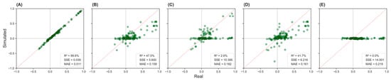
Figure 2.
Simulated versus real correlation values across five input scenarios in the NHANES population. Panels (A–E) display scatter plots comparing the correlation between pairs of variables from simulated data (y-axis) and real data (x-axis). The dashed diagonal line indicates perfect prediction. Panel (A): complete inputs; Panel (B): physician-estimated correlations; Panel (C): literature-based correlations; Panel (D): mixed inputs; Panel (E): no correlations.
3.2. Cardiac Population
The Framingham Heart Study database was used to extract key variables for analysis, including gender, total cholesterol, age, systolic blood pressure, diastolic blood pressure, smoking status, body mass index (BMI), diabetes mellitus, use of antihypertensive medication, heart rate, glucose level, and history of cardiovascular conditions such as previous coronary heart disease (PREVCHD), angina pectoris (PREVAP), myocardial infarction (PREVMI), stroke (PREVSTRK), and hypertension (PREVHYP), as well as the mortality status (DEATH) and education level. The final cohort consisted of 9360 participants. A comparison of summary statistics between the real cohort and all simulated scenarios is presented in Appendix E (Table A2).
Figure 3 displays scatter plots comparing simulated and real-world correlation values across five scenarios (A–E) for the cardiac population. Scenario A (Figure 3A) demonstrates the best agreement between the simulated and actual correlation matrices, with R2 = 86.8%, SSE = 0.709, and MAE = 0.035. Scenario B (Figure 3B), which is based on physician estimates, shows moderate alignment with R2 = 21.9%, SSE = 4.138, and MAE = 0.106. Other scenarios show low agreement, with R2 = 0 to 4.0%.
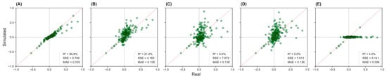
Figure 3.
Simulated versus real correlation values across five input scenarios in the cardiac population. Panels (A–E) display scatter plots comparing the correlation between pairs of variables from simulated data (y-axis) and real data (x-axis). The dashed diagonal line indicates perfect prediction. Panel (A): complete inputs; Panel (B): physician-estimated correlations; Panel (C): literature-based correlations; Panel (D): mixed inputs; Panel (E): no correlations.
3.3. Low-Dimension Population
The low-dimensional population is a subset of the NHANES dataset, including only four key variables: age, gender, body mass index (BMI), and systolic blood pressure (SBP). After excluding individuals with missing data, the final cohort used for this subset consisted of 5866 participants. This reduced dataset was employed as input for the synthetic data generator, with summary statistics comparisons presented in Appendix E (Table A3).
Figure 4 presents the correlation comparison plots across five scenarios (A–E) for the low-dimensional population. Scenario A (Figure 4A) demonstrates the strongest agreement between the synthetic and real-world correlation matrices, with an R2 = 99.4%, SSE = 0.001, and MAE = 0.013. Scenario B (Figure 4B) follows, showing good alignment with R2 = 80.7%, SSE = 0.038, MAE = 0.067. In contrast, Scenario E (Figure 4E) exhibits the weakest performance with R2 = 0.0%, SSE = 0.244, MAE = 0.145, indicating a substantial deviation from the actual correlation structure.
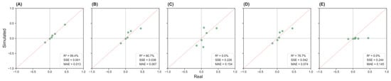
Figure 4.
Simulated versus real correlation values across five input scenarios in the low-dimension population. Panels (A–E) display scatter plots comparing the correlation between pairs of variables from simulated data (y-axis) and real data (x-axis). The dashed diagonal line indicates perfect prediction. Panel (A): complete inputs; Panel (B): physician-estimated correlations; Panel (C): literature-based correlations; Panel (D): mixed inputs; Panel (E): no correlations.
4. Discussion
This study presents a synthetic patient cohort generator designed for health modelling scenarios where complete patient-level data is not available. The method allows users to simulate realistic and clinically valid patient data using only summary statistics and a user-defined correlation matrix. The key advantage of this approach lies in its transparency and configurability: correlations are enforced directly, logical constraints are applied deterministically, and the generation process is fully auditable.
The purpose of our proposed method significantly differs from generative models such as VAEs, GANs, Diffusion Models, or flow matching models, which require large, labeled datasets to learn latent representations of complex data distributions. These methods are not suitable for use in cases where real data is missing, sparse, or aggregated. Moreover, they do not support explicit constraint handling or guarantee the preservation of specific correlations. They inherently depend on learning distributions directly from existing data, implicitly assuming the availability of large and representative datasets; such an approach frequently fails in economic modeling, thus limiting the practicality of these methods when detailed patient-level data are not accessible. For example, ensuring that older age corresponds with higher systolic blood pressure or that only females over 40 can be postmenopausal would require extensive retraining or post-hoc filtering. In our method, these relationships are handled directly and transparently.
Additionally, our study directly challenges the implicit but prevalent assumption in economic modeling practice that uncorrelated synthetic data sufficiently model disease progression. Our simulations, spanning five distinct scenarios across three datasets, clearly demonstrate that incorporating correlation structures—whether sourced from expert input or literature—consistently yields outputs more closely mirroring the intended population characteristics. Even approximate correlations substantially enhance plausibility compared to traditional uncorrelated approaches, reinforcing the practical value of explicitly modeled dependencies.
In our study, we have not quantitatively compared our proposed method with generative models as such an evaluation would not be meaningful due to the fundamentally different purposes served by these methodologies. For example, while a GAN trained on comprehensive datasets such as Framingham may generate realistic patient records, this presupposes full data access and aims for realistic replication. In contrast, our method uniquely supports scenario-based simulations precisely when detailed patient data do not exist. Methodological trade-offs can be thus summarized as follows: generative models excel at producing realistic data from extensive sources but cannot readily enforce specific relationships. Conversely, our approach does not leverage learning from data but crucially allows precise, direct control over desired variable dependencies. A core advantage of the model is its ability to accurately match target values through an iterative mean adjustment process. This ensures that generated data stay within an acceptable range of the user-defined inputs, which is especially important in small-sample simulations where variability can easily skew the results. The model also handles correlation structures effectively using Cholesky decomposition, a stable and efficient method that ensures that the correlation matrix is mathematically valid, even with many variables. Moreover, by resolving parameters in a dependency-aware sequence (e.g., calculating BMI before blood pressure), the generator helps maintain clinical plausibility in simulated data [13].
Importantly, this study indicates that incorporating correlations between variables, whether drawn from expert estimates or published literature, substantially improves the quality of the simulated cohorts. In real-world research, where full datasets may be incomplete or unavailable due to privacy concerns, relying on these estimates is often a practical and preferable solution. Our results clearly demonstrate that preserving correlation structure is crucial: the “no correlation” scenario consistently produced the least realistic outputs across all population types. This emphasizes that adding some form of nearly precise correlation is more effective than assuming that all variables are independent [20].
Another key insight from the validation results is the high performance of expert-informed correlations in comparison to literature-derived matrices. Expert input often outperformed literature-based or mixed matrices, particularly in cardiac and low-dimensional cohorts. This suggests that population-specific clinical insight may offer greater accuracy than generalized published correlations. In contrast, the literature-based matrices, especially when derived from different populations such as Chinese datasets applied to NHANES cohort generation (an American population), sometimes performed worse than using no correlations at all [17,18]. This indicates the critical importance of population-specific context and emphasizes the risk of introducing bias or unrealistic relationships when applying mismatched assumptions in synthetic modeling.
Although our results indicate that physician-estimated correlations often outperformed literature-derived ones, this finding requires cautious interpretation. In our study, physician estimates were averaged from two clinicians, likely reducing individual biases. Notably, despite our experts originating from a different country than the patient data sources, their estimates still demonstrated strong performance, highlighting the usefulness of structured expert input. Inter-rater reliability results reflected good agreement between clinicians, with slightly tighter agreement observed in the Framingham dataset, possibly due to differences in data familiarity, complexity, or variability of the variables assessed. To further enhance consistency, clinical experts were provided with a general framework, future applications may benefit from tailoring this framework to specific modeling contexts. It is also conceivable that literature-based correlations could surpass expert estimates if derived from closely matched populations. However, in practice, such high-quality, population-specific correlations are seldom available, especially in settings characterized by data scarcity or population diversity. Therefore, while acknowledging the potential superiority of literature-based inputs under ideal conditions, expert-derived correlations often represent a more feasible and adaptable choice for real-world modeling applications. Deep generative models may perform well when trained on large, homogeneous datasets from a single population, but their generalizability in health economic applications is often limited. By contrast, our method supports flexible population assumptions, is agnostic to the data source, and can incorporate either empirical or elicited correlation structures with equal ease.
Many existing methods for synthetic data generation prioritize either privacy or realism, often sacrificing one for the other. For example, Data Synthesizer uses differential privacy to protect sensitive information, but this can reduce the variability and utility of the synthetic data for real-world analysis. Generative Adversarial Networks (GANs), which consist of two neural networks competing to produce increasingly realistic data, have been effective in generating synthetic datasets for specific medical conditions like leukemia [21], but their narrow scope limits generalizability. Variational Autoencoders (VAEs), another common method, work by encoding data into a latent space and then decoding it to generate new data. While useful for creating smooth and coherent synthetic samples, VAEs can struggle with high-fidelity generation, especially for complex tabular healthcare data. Moreover, many existing models are evaluated using limited validation strategies and are not tested against real-world datasets [22].
Our patient cohort generator addresses these gaps by allowing users to define specific parameters and generate realistic patient data under different scenarios of data sparsity. Validation through R2 and SSE metrics showed near-perfect matching when accurate correlations were used (e.g., R2 > 99% in the normal and low-dimensional cohorts), reinforcing the tool’s precision in modeling both simple and complex datasets. It is validated using correlation analysis, ensuring both accuracy and applicability for clinical research, while maintaining patient confidentiality.
One of the key practical advantages of our tool is its flexibility. It supports user-defined levels of data sparsity and accommodates correlation matrices informed by expert judgment or the literature, empowering researchers and health policymakers to simulate realistic scenarios even in the absence of real patient data. This makes the generator especially valuable in early-phase feasibility studies, educational simulations, or health policy modeling where control over variable relationships is essential. Moreover, the generator produces interpretable, tabular outputs that mirror conventional epidemiological datasets, making it easier for clinical researchers to validate and work with the simulated data without the need of advanced machine learning expertise.
The accuracy and consistency of expert-derived correlations are critical to the integrity of the simulated data. While we previously recommended that experts be selected from the same clinical and geographic context as the modeled population, we have taken additional measures to ensure quality. Specifically, all participating clinicians were provided with a structured guide (Appendix D) that explained the concept of correlation, offered visual aids, included numeric translation rules, and referenced real-world medical examples to help calibrate their inputs. To evaluate internal consistency, we conducted comparative validation using inputs from each expert individually and in combination (Appendix F, Table A4). Results showed that using the average estimates from multiple experts provided greater stability across simulations. In future applications, the use of structured elicitation methodologies, such as the Delphi method or formal consensus-building techniques, may further enhance the reliability of expert-informed models.
Although the model is hosted within Microsoft Excel, all core calculations are executed via an integrated VBA engine rather than Excel formula functions. This allows for fast in-memory processing, with Excel serving only as a user interface for input configuration and output display. In performance testing using the Framingham dataset, the tool consistently generated a 10,000-patient cohort in under 10 s on a standard commercial laptop (Excel 365 64-bit, Intel Core i7-1365U CPU, 32 GB RAM, no GPU). Even when scaled to 100,000 patients, the tool completed processing in approximately 3 min. Given that synthetic cohort generation is typically a one-time task per modeling or simulation application, the computational burden is minimal and well within acceptable operational limits. While future updates may explore multithreading to further enhance performance during iterative steps, current performance levels do not necessitate such optimization. While the patient cohort generator demonstrates strong performance across various datasets and correlation scenarios, several limitations should be acknowledged. First, the tool currently operates within a static, cross-sectional framework and does not support longitudinal data simulation, limiting its applicability in modeling time-dependent outcomes such as disease progression or treatment response. Second, despite using robust techniques like Cholesky decomposition and expert-informed correlation inputs, the generator relies on predefined parameters and cannot autonomously infer correlations from raw datasets when such data are partially available. Moreover, the reliance on user-provided estimates or literature-derived correlations introduces a potential for bias if the source population does not match the target cohort. The model also currently assumes that the defined constraints and logical rules are exhaustive, which may not capture rare or complex clinical scenarios. Lastly, while implemented in a widely accessible Excel/VBA environment, this platform imposes scalability limitations and may restrict integration with more advanced machine learning pipelines. On the other hand, the underlying logic and conceptual framework are programming-language agnostic, making the tool readily transferable to other environments such as Python or R. The core value lies in the algorithmic structure and methodological rigor, not the implementation platform. Finally, as the method described in the article generates data based on existing statistical information, it is difficult in principle to generate data for completely new diseases or extremely rare patient groups for which no prior research or clinical data exists.
Another important limitation of the current model is its inability to directly reproduce complex non-linear relationships between variables due to the reliance on Cholesky decomposition, which assumes linear dependence. For instance, the cardiovascular risk profile in females undergoes a notable shift around menopause, where associations with variables such as lipid levels or blood pressure may change direction or escalate non-linearly. While the model does not currently handle such dynamics natively, two practical workarounds can be employed. First, the population can be stratified into subgroups where the variable relationships are approximately linear (e.g., premenopausal vs. postmenopausal), and synthetic cohorts can be generated for each subgroup separately before merging them. Second, users can define non-linear relationships using the model’s linking feature, which allows a parameter to be calculated from one or more others using custom equations. While this approach permits complex transformations (e.g., conditional expressions, non-linear scaling), it introduces dependency between variables and may reduce flexibility in certain analyses.
Future developments will focus on expanding the generator’s capabilities to support longitudinal synthetic data generation, enabling the simulation of disease trajectories, treatment pathways, and repeated measures over time. Incorporating multilevel data structures, such as hierarchical models to simulate clusters of patients within hospitals or regions, would further enhance realism for health systems modeling. Another key area of advancement will be the integration of semi-supervised learning to refine correlation matrices based on partial real-world data, reducing dependence on user-supplied inputs. A more scalable implementation in Python or R is also planned to support larger datasets, parallel processing, and integration with AI workflows. Additionally, a user-friendly graphical interface and automated diagnostic tools could facilitate broader adoption among non-technical users.
A fundamental limitation of our method is its reliance on existing statistical summaries, expert knowledge, or clinical literature. Consequently, the model faces inherent challenges in generating synthetic cohorts for completely new or extremely rare conditions lacking any prior data. Future developments could include systematic approaches like Bayesian estimation or expert consensus methodologies (e.g., Delphi technique) to partially address these scenarios.
In our future study, we will address the handling of nonlinear relationships through two distinct methodological approaches. First, we will employ a stratification strategy using the Framingham dataset, targeting correlations that notably change direction or magnitude before and after age 40 in females, such as cardiovascular risk profile factors (e.g., cholesterol levels or blood pressure). The dataset will be stratified into two subgroups—females younger than 40 and those aged 40 or older. We will then separately generate a synthetic cohort for each subgroup before merging them into a combined dataset. Comparative analyses will be performed by calculating metrics for each subgroup individually and for the merged dataset against the original data, explicitly evaluating the method’s capability to accurately capture these reversed correlations. Secondly, we will utilize a linked-equation approach using waist circumference data from NHANES, calculated deterministically from BMI and age using validated clinical formulas. We will compare synthetic cohorts generated with and without deterministic linking, assessing accuracy using statistical metrics such as the mean absolute error (MAE), root mean square error (RMSE), sum of squared errors (SSE), and R2. This evaluation will quantify the improvements in realism and accuracy achieved by employing explicit linking equations. In cases where waist circumference will exhibit linearity, alternative nonlinear clinical equations, such as the Framingham cardiovascular risk scores or renal function equations (MDRD, Cockcroft-Gault), will be identified and tested to further validate the robustness of the linked-equation approach in capturing nonlinear clinical relationships.
Our study aligns with the growing use of synthetic data in healthcare, where access to real patient data is often limited by ethical, regulatory, and institutional constraints. As argued by Duff et al. [23], synthetic datasets provide a privacy-preserving alternative by replicating the statistical properties of real populations, enabling cross-institutional research, algorithm development, and educational simulations without compromising sensitive information. With the increasing adoption of AI in healthcare, simulators capable of generating large-scale, diverse, and clinically coherent data are becoming critical for training, validation, and testing, especially in contexts of data sparsity or population-specific modeling needs.
Beyond technical applications, synthetic data could support broader goals such as data-driven policy development [8]. However, clinical adoption remains cautious due to concerns about data quality, bias, re-identification risk, and provider trust [8]. Regulatory oversight, along with safeguards such as Differential Privacy [24] and dataset provenance tracking [25], will be essential to ensure ethical and responsible deployment.
While we do not compare our method quantitatively against GANs or VAEs in this study, their required inputs and modeling goals differ substantially. These models aim to discover latent features from raw data and replicate its statistical properties in aggregate. Our method instead enables scenario-based modeling in the absence of patient-level data, which is a common requirement in early-stage evaluations, feasibility studies, and constrained research settings.
5. Conclusions
This study presents a reliable and versatile tool for generating synthetic patient cohorts that mirror real-world data structures. It provides a structured simulation framework that maintains control over input assumptions, enforces logical coherence, and supports expert-driven modeling when empirical data are unavailable. The results emphasize that including population-relevant correlations, especially those informed by clinical experts, substantially improves the realism and fidelity of synthetic datasets. The tool is not only technically sound but also accessible to healthcare professionals with limited statistical or coding experience, making it highly applicable across diverse research and policy contexts.
Supplementary Materials
The following supporting information can be downloaded at: https://www.mdpi.com/article/10.3390/a18080475/s1, S1 Summary statistics of means, standard deviations, parameter bounds, and pairwise correlations.
Author Contributions
Conceptualization, A.N.F. and K.E.; methodology, A.N.F., R.A., K.E., B.N. (Bertalan Nemeth), D.N., B.N. (Balazs Nagy) and Z.V.; software, A.N.F., R.A., K.E., B.N. (Bertalan Nemeth), D.N. and B.N. (Balazs Nagy); validation, A.N.F., R.A., A.I. and B.N. (Bertalan Nemeth); formal analysis, A.N.F., R.A. and K.E.; investigation, A.N.F., R.A. and K.E.; resources, A.N.F. and K.E.; data curation, A.N.F., R.A. and K.E.; writing—original draft, A.N.F., R.A., R.H. and A.I.; writing—review and editing, A.N.F., R.A., R.H., K.E., A.I., B.N. (Bertalan Nemeth), D.N., B.N. (Balazs Nagy) and Z.V.; visualization, A.N.F., R.A. and A.I.; project administration, A.N.F. and R.H.; supervision, R.H., B.N. (Balazs Nagy) and Z.V.; funding acquisition, R.H. All authors have read and agreed to the published version of the manuscript.
Funding
This research received no external funding.
Informed Consent Statement
This study used publicly available, de-identified data (NHANES 2021–2023, Framingham Heart Study) to generate synthetic patient cohorts for validation. No human subjects were involved, and ethical approval was not required. Data handling followed legal and ethical guidelines. Synthetic data, created via statistical simulation, cannot be linked to real individuals.
Data Availability Statement
The real-world datasets used for validation (NHANES and Framingham Heart Study) are publicly available from the U.S. Centers for Disease Control and Prevention (https://wwwn.cdc.gov/nchs/nhanes/continuousnhanes/default.aspx?Cycle=2021-2023; accessed on 29 July 2025) and the National Heart, Lung, and Blood Institute (https://www.kaggle.com/code/dessanriv/framingham-heart-study; accessed on 29 July 2025). The synthetic datasets generated during the current study are available from the corresponding author upon reasonable request.
Acknowledgments
The authors acknowledge the U.S. CDC and NHLBI for maintaining and providing access to the NHANES and Framingham datasets, respectively.
Conflicts of Interest
Kareem ElFass is an employee of Syreon Middle East. The authors declare no conflicts of interest.
Abbreviations
The following abbreviations are used in this manuscript:
| API | Application Programming Interface |
| BMI | Body Mass Index |
| CDF | Cumulative Distribution Function |
| GAN’s | Generative Adversarial Networks |
| EHR | Electronic Health Record |
| IF | Conditional Function (Excel or programming logic function) |
| MAE | Mean Absolute Error |
| MSE | Mean Squared Error |
| NHANES | National Health and Nutrition Examination Survey |
| R2 | Coefficient of Determination |
| RMSE | Root Mean Squared Error |
| SBP | Systolic Blood Pressure |
| SD | Standard Deviation |
| SSE | Sum of Squared Errors |
| U(0,1) | Uniform Distribution between 0 and 1 |
| VBA | Visual Basic for Applications |
| VAEs | Variational Autoencoders |
| Z | Z-score (Standardized Score) |
Appendix A. Parsing and Resolving Hard Limits and Linked Equations
In this section, we outline explicit steps for parsing and evaluating user-defined hard limits and linked equations, along with illustrative examples.
Appendix A.1. Resolving Hard Limits
Hard limits are user-defined logical conditions that determine the eligibility of specific patient characteristics, ensuring biological and logical plausibility within the synthetic cohort. Each parameter may have an associated hard limit expressed as a logical formula, provided as a string by the user. These formulas incorporate short parameter names and standard logical functions, including the following:
- Logical operators: AND(), OR(), IF()
- Comparison operators: >, <, =, <>
Example Scenario
Menopause: “and (Female = 1, Age > 40)” ensures menopause only applies to females over 40.
Pregnancy: “and (Female = 1, Age > 15, Age < 50)” restricts pregnancy to females aged 15–50.
Smoking Status: “Age ≥ 12” ensures no patient under 12 years old is assigned smoking status.
Steps to resolve hard limits for each parameter and each patient are as follows:
- Substitution: Replace parameter names within the formula with actual patient-specific values.Example:
- Patient 1: Age = 35, Female = 1
- Formula: and (Female = 1, Age > 40)
- Substituted: and (1 = 1, 35 > 40)
- Evaluation: Assess the substituted formula logically.
- Result: and (TRUE, FALSE) → FALSE
- Assignment: If the formula evaluates to FALSE, set the parameter value to zero (Xi = 0).
This procedure ensures that no biologically impossible or inconsistent patient characteristic is assigned.
Appendix A.2. Computing Linked Parameters
Linked parameters are not randomly generated; rather, they are computed based on other patient variables via user-defined equations. This ensures logical consistency, deterministic relationships, and avoids redundant or inconsistent data. Characteristics of linked parameters are as follows:
- Logical Consistency: Parameters such as BMI categories derived from continuous BMI values.
- Deterministic Relationships: Variables computed from known relationships (e.g., Heart Rate Variability dependent on Age and Physical Activity).
- Avoidance of Redundancy: Derived risk scores dependent on multiple patient variables.
Example Scenario
BMI Category: if (BMI < 18.5, “Underweight”, if (BMI < 25,“Normal”, if (BMI < 30, “Overweight”, “Obese”)))
Hypertension Status: if (SBP > 140,1,0)
Cardiovascular Risk Score: (Age * 0.1) + (SBP * 0.2) + (Diabetes * 1.5)
Steps to Resolve Linked Parameters for each linked parameter and each patient are as follows:
- Substitution: Replace parameter names in the linking equation with actual patient-specific values.Example:
- Patient 1: Age = 60, SBP = 150, Diabetes = 1
- Formula: (Age * 0.1) + (SBP * 0.2) + (Diabetes * 1.5)
- Substituted: (60 * 0.1) + (150 * 0.2) + (1 * 1.5)
- Evaluation: Compute mathematical or logical operation.
- Result: 6 + 30 + 1.5 → 37.5
- Assignment: Assign the computed value to the linked parameter.
This ensures that linked parameters are accurately derived, maintaining internal consistency and clinical plausibility within the synthetic patient cohort.
Appendix B. Parameter Estimation for Distribution Functions
To accurately simulate patient characteristics using various statistical distributions, the model calculates distribution-specific parameters—such as shape (α) and scale (λ)—using the user-provided mean (μ) and standard deviation (σ). The formulas vary by distribution type as follows:
- Gamma Distribution
- Shape (α):
- Scale (λ):
- Beta Distribution
- Shape α:
- Shape β:
Note: Only α is derived in the original function, with β computed via if needed.
- 3.
- Log-Normal Distribution
- Mean of log (μ_log):
- Standard deviation of log (σ_log):
- 4.
- Normal Distribution
- Mean (α):
- Standard Deviation (λ):
These equations ensure the accurate parameterization of distribution functions, facilitating valid stochastic sampling, particularly for the inverse cumulative distribution (quantile) functions used in simulations and probabilistic modeling
Appendix C. Constructing and Resolving the Dependency Matrix Importance of Parameter Resolution Order
In this section, we provide a detailed description of constructing and resolving the dependency matrix—including algorithmic steps, examples, and the handling of circular dependencies. In the cohort-generation model, the sequence in which parameters are computed is essential for logical consistency and clinical plausibility. This sequence is especially critical when the model employs user-defined hard limits or linked equations, creating explicit dependencies among parameters, for instance, the following:
- Menopause cannot be resolved before knowing both age and sex.
- Hypertension diagnosis depends upon previously computed values, such as systolic blood pressure (SBP).
Appendix C.1. Constructing the Dependency Matrix
To establish the correct computation order, the model constructs a binary dependency matrix. Each entry D_(i,j) indicates whether parameter i depends on parameter j:
D_(i,j) = 1, if parameter i depends on parameter, otherwise D_(i,j) = 0
This matrix is built by analyzing user-provided formulas:
- Hard Limit Rules—conditions defining when a parameter can take specific values.
- Linking Equations—expressions computing one parameter based on others.
An example of a dependency matrix is as follows:
| Parameter | Age | Sex | Menopause | SBP | Hypertension |
| Age | 0 | 0 | 0 | 0 | 0 |
| Sex | 0 | 0 | 0 | 0 | 0 |
| Menopause | 1 | 1 | 0 | 0 | 0 |
| SBP | 1 | 0 | 0 | 0 | 0 |
| Hypertension | 0 | 0 | 0 | 1 | 0 |
- Menopause depends on age and sex.
- SBP depends only on age.
- Hypertension depends on SBP.
Appendix C.2. Determining Parameter Dependency Levels
Once the dependency matrix is constructed, parameters are assigned a dependency level through an iterative algorithm, ensuring all dependencies are accounted for. Algorithm steps are as follows:
- Initialize all parameters with a dependency level of 0 (unresolved).
- Iterate through parameters until all have an assigned level:
- ○
- Skip parameters already assigned a level.
- ○
- For unresolved parameters, check dependencies:
- If any dependencies are unresolved, skip the parameter.
- If all dependencies are resolved, assign a dependency level one higher than its highest dependency.
- Continue until every parameter has an assigned dependency level.
Appendix C.3. Levels Explanation
Level 1: Independent parameters (no dependencies).
Level 2: Parameters dependent only on Level 1 parameters.
Level 3: Parameters dependent on Level 2 parameters.
And so forth, up to the number of parameters.
Appendix C.4. Detecting Circular Dependencies
The algorithm checks for circular dependencies (e.g., Parameter A depends on B, and B depends on A or even indirectly):
- If any parameter remains unresolved after iterative resolution (dependency level remains 0), a circular dependency exists.
- The algorithm flags an error and stops execution for correction.
We illustrate this approach using an example of dependency resolution in practice. Given the previous dependency matrix, the resolution order is as follows:
| Parameter | Depends On | Dependency Level |
| Age | None | 1 |
| Sex | None | 1 |
| SBP | Age | 2 |
| Menopause | Age, Sex | 2 |
| Hypertension | SBP | 3 |
Resolution sequence is then as follows:
Level 1: Resolve Age, Sex
Level 2: Resolve SBP, Menopause
Level 3: Resolve Hypertension
This structured approach ensures logical coherence, clinical plausibility, and accurate, consistent patient cohort generation.
Appendix D. Correlation Estimation and Interpretation by a Clinical Expert
In this section, we outline the reference guide, which was followed by a clinical expert in correlation estimation and interpretation. It is important to note that the expert guidance provided is a general framework and not a rigid protocol. We fully acknowledge that practitioners may identify opportunities for case-specific improvements.
Clinical Expert Reference Guide for Correlation Estimation and Interpretation
- Purpose of the Correlation Matrix
We are asking you, as a clinical expert, to assess the relationships between health-related variables based on your clinical knowledge and experience with a specific patient population. These assessments will be used to build a scientific model that reflects real-world clinical patterns. You do not need to perform any calculations, just provide your judgment about whether each pair of variables is related, and if so, how strongly and in which direction.
- 2.
- What Is Correlation?
Correlation tells us how closely two variables move together in a linear pattern:
Positive Correlation: When one variable increases, the other tends to increase as well.
Negative Correlation: When one variable increases, the other tends to decrease.
No Correlation: No consistent or meaningful pattern exists between the two variables.
- 3.
- Key Concept: Scatter Determines Correlation (Not Slope)
When visualized on a graph (called a scatter plot), each pair of values (e.g., age and blood pressure) is shown as a dot. The correlation strength depends on how tightly the dots cluster around an imaginary straight line.
- 4.
- How to Fill the Matrix
For each pair of variables in the matrix:
Step 1: Think About the Direction
Do both variables tend to increase or decrease together? → Positive
Does one tend to increase while the other decreases? → Negative
Not sure, or no consistent pattern in your experience? → No/Unsure
Step 2: Think About the Strength
If you choose Positive or Negative, assess how consistent this relationship is:
| Strength | Your Clinical Interpretation |
| Weak | Slight trend, many exceptions |
| Moderate | Clear trend, but not always consistent |
| Strong | Very consistent relationship in most or all patients |
- 5.
- Translation into Numeric Values
Your input will be translated into numerical values for analysis as follows:
| Clinical Input | Numeric Value |
| No/Unsure | 0.00 |
| Weak Positive | +0.15 |
| Moderate Positive | +0.25 |
| Strong Positive | +0.55 |
| Weak Negative | −0.15 |
| Moderate Negative | −0.25 |
| Strong Negative | −0.55 |
Appendix E. Comparisons Between Real-World Datasets and Synthetic Cohorts
Table A1, Table A2 and Table A3 present detailed comparisons of summary statistics between real-world datasets and synthetic cohorts for all five generation scenarios across three patient populations: general (NHANES), cardiac (Framingham Heart Study), and low-dimensional (NHANES subset). Table A4 provides correlation fit metrics comparing estimates of two clinical expert and their average in synthetic data generation. These comparisons validate the fundamental statistical fidelity of the patient cohort generator, demonstrating its accuracy in reproducing central tendencies and variability across diverse clinical variables. The inclusion of p-values confirms the statistical equivalence between real and synthetic datasets, demonstrating that the tool reliably maintains individual variable distributions. Presenting these foundational validation tables is essential, as they establish the baseline accuracy required for further advanced validations, including the preservation of inter-variable correlations.
The comparisons revealed near-perfect agreement in means and standard deviations across all variables and scenarios. For every variable assessed, the generated synthetic values remained statistically indistinguishable from the real-world reference data, with p-values consistently exceeding 0.90. In many instances, notably within the Framingham cohort (Table A2), p-values reached 1.000 across all variables and scenarios. This suggests the generator’s exceptional capacity to match target input distributions with high fidelity, even in large and complex cohorts.
This trend held true across all simulation scenarios, including Scenario E, which lacked any correlation inputs. While this scenario performed poorly in terms of preserving inter-variable relationships, it nonetheless produced synthetic datasets with central tendency and dispersion metrics closely matching those of the real cohort. This highlights a key limitation of summary statistics alone as a validation metric. Many existing synthetic data generators are capable of replicating marginal distributions (e.g., mean and standard deviation) by design. As such, achieving agreement in summary statistics is necessary, but insufficient, to claim realism in synthetic data. Consequently, our model’s primary validation focused on preserving correlation structures and clinical plausibility.
Interestingly, while the Framingham cohort showed virtually no variation in p-values across scenarios, the NHANES normal population cohort exhibited slightly lower—though still non-significant—p-values. This variation may be attributable to the distributional assumptions used. The NHANES simulations predominantly relied on log-normal distributions, whereas Framingham scenarios employed a mix of normal and gamma distributions. Conversely, the low-dimensional NHANES cohort achieved perfect p-values across scenarios despite also using log-normal distributions. This suggests that smaller parameter sets can yield highly accurate and reliable synthetic results, even under skewed distributions.
Moreover, the NHANES general population cohort included deterministic logical constraints—making it unique among test groups. Despite this added complexity, the synthetic data remained statistically consistent with the real dataset, affirming the robustness of the generator’s constraint-resolution logic.
Finally, binary and categorical variables, particularly those in the Framingham dataset, were replicated with absolute precision across all simulations. As reflected in Table A2, binary prevalence rates and categorical distributions matched exactly with their real-world counterparts. This underscores the algorithm’s efficacy in handling non-continuous parameters using its percentile-thresholding method and validates its deterministic approach to preserving prevalence and logical constraints in categorical data.
Overall, while strong performance in matching the mean and standard deviation is a foundational requirement for any synthetic data tool, the distinctive strength of our model lies in its capacity to go beyond basic summary statistics and emulate the structural interdependencies characteristic of real-world data.
Table A1.
Summary statistics of NHANES real data versus five scenarios. The test of significance used is the Chi-square test for nominal variables and ANOVA for continuous variables. The level of significance applied is p < 0.05.
Table A1.
Summary statistics of NHANES real data versus five scenarios. The test of significance used is the Chi-square test for nominal variables and ANOVA for continuous variables. The level of significance applied is p < 0.05.
| Variable, Mean (SD) | Real Data | Scenario A | Scenario B | Scenario C | Scenario D | Scenario E | p-Value |
|---|---|---|---|---|---|---|---|
| N | 5866 | 5866 | 5866 | 5866 | 5866 | 5866 | |
| Age (years) | 48.33 (20.67) | 48.33 (18.62) | 48.33 (18.62) | 48.33 (18.62) | 48.33 (18.62) | 48.33 (18.62) | 1.000 |
| Weight (kg) | 80.64 (21.65) | 80.25 (22.27) | 80.25 (22.27) | 80.25 (22.27) | 80.25 (22.27) | 80.25 (22.27) | 0.911 |
| Height (cm) | 166.90 (9.98) | 166.75 (10.02) | 166.75 (10.02) | 166.75 (10.01) | 166.75 (10.02) | 166.75 (10.01) | 0.956 |
| Body mass index | 28.85 (6.97) | 28.76 (7.19) | 28.76 (7.04) | 28.76 (6.92) | 28.76 (7.04) | 28.76 (6.94) | 0.972 |
| Upper leg length | 38.55 (3.60) | 38.56 (3.59) | 38.56 (3.59) | 38.56 (3.57) | 38.56 (3.59) | 38.56 (3.57) | 1.000 |
| Upper arm length | 37.52 (2.91) | 37.48 (2.92) | 37.48 (2.94) | 37.48 (2.95) | 37.48 (2.94) | 37.48 (2.95) | 0.964 |
| Arm circumference | 32.95 (5.25) | 32.87 (5.49) | 32.87 (5.35) | 32.87 (5.28) | 32.87 (5.35) | 32.87 (5.28) | 0.949 |
| Waist circumference | 98.24 (17.41) | 97.90 (17.87) | 97.90 (17.82) | 97.90 (17.16) | 97.90 (17.80) | 97.90 (17.62) | 0.868 |
| Hip circumference | 106.19 (13.96) | 105.96 (14.22) | 105.96 (14.00) | 105.96 (13.96) | 105.95 (14.00) | 105.96 (13.92) | 0.927 |
| Systolic blood pressure | 120.61 (18.11) | 120.50 (18.31) | 120.50 (18.39) | 120.50 (18.25) | 120.50 (18.39) | 120.50 (18.52) | 0.999 |
| Diastolic blood pressure | 73.78 (11.48) | 73.64 (11.77) | 73.64 (11.69) | 73.64 (11.72) | 73.64 (11.69) | 73.64 (11.59) | 0.985 |
| Pulse | 71.29 (12.21) | 71.43 (12.37) | 71.43 (12.39) | 71.43 (12.41) | 71.43 (12.39) | 71.43 (12.41) | 0.985 |
| High density lipoprotein (mg/dL) | 54.19 (14.27) | 54.19 (14.23) | 54.19 (14.21) | 54.19 (14.07) | 54.19 (13.92) | 54.19 (14.25) | 1.000 |
| Total cholesterol (mg/dL) | 183.82 (42.41) | 183.82 (41.72) | 183.82 (42.01) | 183.82 (41.63) | 183.82 (42.18) | 183.84 (41.49) | 1.000 |
| White blood cell count (1000 cells/uL) | 6.87 (1.98) | 6.87 (1.97) | 6.87 (1.97) | 6.87 (1.96) | 6.87 (4.83) | 6.87 (1.97) | 1.000 |
| Hemoglobin (g/dL) | 13.89 (1.45) | 13.89 (1.47) | 13.89 (1.46) | 13.89 (1.46) | 13.89 (4.15) | 13.89 (1.46) | 1.000 |
| High-sensitivity C reactive protein (mg/L) | 3.50 (7.12) | 3.50 (6.99) | 3.50 (6.91) | 3.50 (7.30) | 3.50 (3.39) | 3.50 (7.32) | 1.000 |
Table A2.
Summary statistics of Framingham real data versus five scenarios. The test of significance used is the Chi-square test for nominal variables and ANOVA for continuous variables. The level of significance applied is p < 0.05.
Table A2.
Summary statistics of Framingham real data versus five scenarios. The test of significance used is the Chi-square test for nominal variables and ANOVA for continuous variables. The level of significance applied is p < 0.05.
| Variable | Real Data | Scenario A | Scenario B | Scenario C | Scenario D | Scenario E | p-Value |
|---|---|---|---|---|---|---|---|
| N | 9360 | 9360 | 9360 | 9360 | 9360 | 9360 | |
| Sex (Male) | 4152 (44.4) | 4152 (44.4) | 4152 (44.4) | 4152 (44.4) | 4152 (44.4) | 4152 (44.4) | 1.000 |
| Total cholesterol, mean (SD) | 241.56 (45.17) | 241.55 (45.01) | 241.55 (45.06) | 241.55 (45.08) | 241.55 (45.08) | 241.55 (45.06) | 1.000 |
| Age, mean (SD) | 54.25 (9.45) | 54.25 (9.25) | 54.25 (9.26) | 54.25 (9.25) | 54.25 (9.25) | 54.25 (9.23) | 1.000 |
| SBP, mean (SD) | 135.72 (22.59) | 135.72 (22.44) | 135.72 (22.43) | 135.73 (22.48) | 135.73 (22.48) | 135.72 (22.39) | 1.000 |
| DBP, mean (SD) | 82.93 (11.75) | 82.93 (11.82) | 82.93 (11.68) | 82.93 (11.66) | 82.93 (11.66) | 82.93 (11.61) | 1.000 |
| Current smoker, yes, n (%) | 5246 (56.0) | 5246 (56.0) | 5246 (56.0) | 5246 (56.0) | 5246 (56.0) | 5246 (56.0) | 1.000 |
| BMI, mean (SD) | 25.81 (4.03) | 25.81 (4.07) | 25.81 (4.04) | 25.81 (4.03) | 25.81 (4.03) | 25.81 (4.07) | 1.000 |
| Diabetes, No, n (%) | 8968 (95.8) | 8968 (95.8) | 8968 (95.8) | 8968 (95.8) | 8968 (95.8) | 8968 (95.8) | 1.000 |
| BPMEDS, No | 8582 (91.7) | 8582 (91.7) | 8582 (91.7) | 8582 (91.7) | 8582 (91.7) | 8582 (91.7) | 1.000 |
| Heart rate, mean (SD) | 76.76 (12.35) | 76.76 (12.47) | 76.76 (12.41) | 76.76 (9.76) | 76.76 (10.02) | 76.76 (12.39) | 1.000 |
| Blood sugar level, mean (SD) | 83.77 (25.06) | 83.77 (24.34) | 83.77 (24.44) | 83.77 (12.44) | 83.77 (12.95) | 83.77 (24.36) | 1.000 |
| CHD, No, n (%) | 8725 (93.2) | 8725 (93.2) | 8725 (93.2) | 8725 (93.2) | 8725 (93.2) | 8725 (93.2) | 1.000 |
| Angina, No, n (%) | 8889 (95.0) | 8889 (95.0) | 8889 (95.0) | 8889 (95.0) | 8889 (95.0) | 8889 (95.0) | 1.000 |
| Myocardial infarction, No, n (%) | 9065 (96.8) | 9065 (96.8) | 9065 (96.8) | 9065 (96.8) | 9065 (96.8) | 9065 (96.8) | 1.000 |
| Stroke, No, n (%) | 9243 (98.8) | 9243 (98.8) | 9243 (98.8) | 9243 (98.8) | 9243 (98.8) | 9243 (98.8) | 1.000 |
| Hypertension, No, n (%) | 5180 (55.3) | 5180 (55.3) | 5180 (55.3) | 5180 (55.3) | 5180 (55.3) | 5180 (55.3) | 1.000 |
| Death, No, n (%) | 6556 (70.0) | 6556 (70.0) | 6556 (70.0) | 6556 (70.0) | 6556 (70.0) | 6556 (70.0) | 1.000 |
| Education1, n (%) | 3814 (40.7) | 3814 (40.7) | 3814 (40.7) | 3814 (40.7) | 3814 (40.7) | 3814 (40.7) | 1.000 |
| Education2, n (%) | 2836 (30.3) | 2836 (30.3) | 2836 (30.3) | 2836 (30.3) | 2836 (30.3) | 2836 (30.3) | 1.000 |
| Education3, n (%) | 1566 (16.7) | 1566 (16.7) | 1566 (16.7) | 1566 (16.7) | 1566 (16.7) | 1566 (16.7) | 1.000 |
| Education4, n (%) | 1144 (12.2) | 1144 (12.2) | 1144 (12.2) | 1144 (12.2) | 1144 (12.2) | 1144 (12.2) | 1.000 |
Table A3.
Summary statistics of low dimension NHANES real data versus five scenarios. The test of significance used is the Chi-square test for nominal variables and ANOVA for continuous variables. The level of significance applied is p < 0.05.
Table A3.
Summary statistics of low dimension NHANES real data versus five scenarios. The test of significance used is the Chi-square test for nominal variables and ANOVA for continuous variables. The level of significance applied is p < 0.05.
| Variable | Real Data | Scenario A | Scenario B | Scenario C | Scenario D | Scenario E | p-Value |
|---|---|---|---|---|---|---|---|
| N | 5866 | 5866 | 5866 | 5866 | 5866 | 5866 | |
| Sex, Male, n (%) | 2707 (46.1) | 2707 (46.1) | 2707 (46.1) | 2707 (46.1) | 2707 (46.1) | 2707 (46.1) | 1.000 |
| Age, year, mean (SD) | 48.33 (20.67) | 48.33 (18.81) | 48.33 (18.82) | 48.33 (18.82) | 48.33 (18.82) | 48.33 (18.82) | 1.000 |
| BMI, mean (SD) | 28.85 (6.97) | 28.85 (6.93) | 28.85 (6.93) | 28.85 (6.95) | 28.85 (6.93) | 28.85 (6.95) | 1.000 |
| SBP, mean (SD) | 120.61 (18.11) | 120.61 (17.97) | 120.61 (17.97) | 120.61 (18.03) | 120.61 (17.96) | 120.61 (17.77) | 1.000 |
Appendix F. Assessment of Expert-Derived Correlations
To assess the reliability of expert-derived correlations, we conducted a comparative analysis of synthetic data generated using inputs from the following:
- Clinical Expert A alone,
- Clinical Expert B alone,
- The combined average of both.
Table A4 shows that the performance of expert-derived correlations varied across scenarios. In the Normal population, Expert A clearly outperformed Expert B across all metrics (e.g., RMSE: 0.216 vs. 0.387; R2: 0.404 vs. −0.906), yet the combined average yielded even better results (RMSE: 0.203; R2: 0.475). In the Cardiac scenario, Expert B performed better than Expert A (RMSE: 0.159 vs. 0.211), but again, the combined average improved further (RMSE: 0.141; R2: 0.219). For the low-dimension setting, Expert B showed the best individual performance (RMSE: 0.101; R2: 0.949), yet averaging still slightly enhanced RMSE (0.080) with a high R2 (0.807).
Table A4.
Correlation fit metrics comparing two expert estimates and their average in synthetic data generation.
Table A4.
Correlation fit metrics comparing two expert estimates and their average in synthetic data generation.
| Population | Scenario | MAE | MSE | RMSE | R2 | SSE |
|---|---|---|---|---|---|---|
| Normal | Clinical Expert A | 0.163 | 0.047 | 0.216 | 0.404 | 6.361 |
| Clinical Expert B | 0.286 | 0.149 | 0.387 | −0.906 | 20.327 | |
| Combined average of both | 0.158 | 0.041 | 0.203 | 0.475 | 5.600 | |
| Cardiac | Clinical Expert A | 0.149 | 0.044 | 0.211 | −0.742 | 9.330 |
| Clinical Expert B | 0.110 | 0.025 | 0.159 | 0.013 | 5.286 | |
| Combined average of both | 0.106 | 0.020 | 0.141 | 0.219 | 4.183 | |
| Low Dimension | Clinical Expert A | 0.165 | 0.062 | 0.248 | −0.879 | 0.370 |
| Clinical Expert B | 0.087 | 0.010 | 0.101 | 0.949 | 0.010 | |
| Combined average of both | 0.067 | 0.006 | 0.080 | 0.807 | 0.038 |
Inter-Rater Agreement in Expert-Derived Correlation Estimation
To evaluate the consistency between two clinical experts in estimating the correlation structures used for synthetic data generation, we assessed both the Intraclass Correlation Coefficient (ICC) and the Concordance Correlation Coefficient (CCC) across two reference datasets (NHANES and Framingham). We selected the ICC from a two-way random-effects model for average ratings, which reflects the reliability of using the average of both experts’ estimates. Table A5 shows that the inter-rater agreement was excellent in the NHANES dataset (ICC = 0.892; CCC = 0.804) and moderate in Framingham (ICC = 0.589; CCC = 0.409). Despite variation in individual expert accuracy, the averaged correlations consistently delivered the best overall synthetic data quality. The strong agreement in NHANES justifies this averaging approach, while the moderate agreement in Framingham suggests that averaging still helps mitigate expert variability and enhances model reliability.
Table A5.
Agreement metrics between two clinical experts in correlation estimation.
Table A5.
Agreement metrics between two clinical experts in correlation estimation.
| Dataset | ICC | CCC (95% CI) | Agreement Interpretation |
|---|---|---|---|
| NHANES | 0.892 | 0.804 (0.733–0.858) | Excellent agreement with minimal bias |
| Framingham | 0.589 | 0.409 (0.278–0.526) | Moderate agreement with higher variability |
References
- Gonzales, A.; Guruswamy, G.; Smith, S.R. Synthetic data in health care: A narrative review. PLoS Digit. Health 2023, 2, e0000082. [Google Scholar] [CrossRef] [PubMed]
- Kimko, H.; Lee, K. Improving Realism in Clinical Trial Simulations via Real-World Data. CPT Pharmacomet. Syst. Pharmacol. 2017, 6, 727–729. [Google Scholar] [CrossRef] [PubMed]
- Pezoulas, V.C.; Zaridis, D.I.; Mylona, E.; Androutsos, C.; Apostolidis, K.; Tachos, N.S.; Fotiadis, D.I. Synthetic data generation methods in healthcare: A review on open-source tools and methods. Comput. Struct. Biotechnol. J. 2024, 23, 2892–2910. [Google Scholar] [CrossRef] [PubMed]
- Li, J.; Guo, S.; Ma, R.; He, J.; Zhang, X.; Rui, D.; Ding, Y.; Li, Y.; Jian, L.; Cheng, J.; et al. Comparison of the effects of imputation methods for missing data in predictive modelling of cohort study datasets. BMC Med. Res. Methodol. 2024, 24, 1–9. [Google Scholar] [CrossRef] [PubMed]
- Ochoa-Muñoz, A.F.; Contreras-Reyes, J.E. Multiple Factor Analysis Based on NIPALS Algorithm to Solve Missing Data Problems. Algorithms 2023, 16, 457. [Google Scholar] [CrossRef]
- Kühnel, L.; Schneider, J.; Perrar, I.; Adams, T.; Moazemi, S.; Prasser, F.; Nöthlings, U.; Fröhlich, H.; Fluck, J. Synthetic data generation for a longitudinal cohort study-evaluation, method extension and reproduction of published data analysis results. Sci. Rep. 2024, 14, 14412. [Google Scholar] [CrossRef] [PubMed]
- Mendes, J.M.; Barbar, A.; Refaie, M. Synthetic data generation: A privacy-preserving approach to accelerate rare disease research. Front. Digit. Health 2025, 7, 1563991. [Google Scholar] [CrossRef] [PubMed]
- Giuffrè, M.; Shung, D.L. Harnessing the power of synthetic data in healthcare: Innovation, application, and privacy. NPJ Digit. Med. 2023, 6, 186. [Google Scholar] [CrossRef] [PubMed]
- Miletic, M.; Sariyar, M. Utility-based Analysis of Statistical Approaches and Deep Learning Models for Synthetic Data Generation with Focus on Correlation Structures: Algorithm Development and Validation. JMIR AI 2025, 4, e65729. [Google Scholar] [CrossRef] [PubMed]
- Subramanian, S.; Rajeswar, S.; Dutil, F.; Pal, C.; Courville, A. Adversarial Generation of Natural Language. In Proceedings of the 2nd Workshop on Representation Learning for NLP; ACL: Vancouver, BC, Canada, 2017; pp. 241–251. [Google Scholar]
- Ren, Y.; Lin, J.; Tang, S.; Zhou, J.; Yang, S.; Qi, Y.; Ren, X. Generating Natural Language Adversarial Examples on a Large Scale with Generative Models. Front. Artif. Intell. Appl. 2020, 325, 2156–2163. [Google Scholar]
- Liu, M.Y.; Huang, X.; Yu, J.; Wang, T.-C.; Mallya, A. Generative Adversarial Networks for Image and Video Synthesis: Algorithms and Applications. Proc. IEEE 2021, 109, 839–862. [Google Scholar] [CrossRef]
- Marchev, A.; Marchev, V. Automated Algorithm for Multi-variate Data Synthesis with Cholesky Decomposition. In Proceedings of the 7th International Conference on Algorithms, Computing and Systems, Larissa, Greece, 19–21 October 2023; pp. 1–6. [Google Scholar]
- Van De Geijn, R.A. Notes on Cholesky Factorization 1 Definition and Existence; Report TX, 78712; University of Texas: Austin, TX, USA, 2014. [Google Scholar]
- Solow, A.R. Bootstrapping correlated data. J. Int. Assoc. Math. Geol. 1985, 17, 769–775. [Google Scholar] [CrossRef]
- Schumm, W.R. Patterns of Means and Standard Deviations with Binary Variables: A Key to Detecting Fraudulent Research. Biomed. J. Sci. Tech. Res. 2019, 23, 17151–17153. [Google Scholar] [CrossRef]
- Wang, H.; Shuai, P.; Deng, Y.; Yang, J.; Shi, Y.; Li, D.; Yong, T.; Liu, Y.; Huang, L. A correlation-based feature analysis of physical examination indicators can help predict the overall underlying health status using machine learning. Sci. Rep. 2022, 12, 19626. [Google Scholar] [CrossRef] [PubMed]
- NHANES Questionnaires, Datasets, and Related Documentation. Available online: https://wwwn.cdc.gov/nchs/nhanes/continuousnhanes/default.aspx?Cycle=2021-2023 (accessed on 29 May 2025).
- Framingham Heart Study. Available online: https://www.kaggle.com/code/dessanriv/framingham-heart-study (accessed on 29 May 2025).
- Tedersoo, L.; Küngas, R.; Oras, E.; Köster, K.; Eenmaa, H.; Leijen, Ä.; Pedaste, M.; Raju, M.; Astapova, A.; Lukner, H.; et al. Data sharing practices and data availability upon request differ across scientific disciplines. Sci. Data 2021, 8, 192. [Google Scholar] [CrossRef] [PubMed]
- Chen, X.; Wu, Z.; Shi, X.; Cho, H.; Mukherjee, B. Generating Synthetic Electronic Health Record (EHR) Data: A Review with Benchmarking. arXiv 2024, arXiv:2411.04281. [Google Scholar]
- Goyal, M.; Mahmoud, Q.H. A Systematic Review of Synthetic Data Generation Techniques Using Generative AI. Electronics 2024, 13, 3509. [Google Scholar] [CrossRef]
- McDuff, D.; Curran, T.; Kadambi, A. Synthetic Data in Healthcare. arXiv 2023, arXiv:2304.03243. [Google Scholar]
- Mulder, V.; Humbert, M. Differential privacy. In Trends in Data Protection and Encryption Technologies; Springer: Berlin/Heidelberg, Germany, 2023; pp. 157–161. [Google Scholar]
- Magagna, B.; Goldfarb, D.; Martin, P.; Atkinson, M.; Koulouzis, S.; Zhao, Z. Data provenance. In Towards Interoperable Research Infrastructures for Environmental and Earth Sciences; Springer: Berlin/Heidelberg, Germany, 2020; pp. 208–225. [Google Scholar]
Disclaimer/Publisher’s Note: The statements, opinions and data contained in all publications are solely those of the individual author(s) and contributor(s) and not of MDPI and/or the editor(s). MDPI and/or the editor(s) disclaim responsibility for any injury to people or property resulting from any ideas, methods, instructions or products referred to in the content. |
© 2025 by the authors. Licensee MDPI, Basel, Switzerland. This article is an open access article distributed under the terms and conditions of the Creative Commons Attribution (CC BY) license (https://creativecommons.org/licenses/by/4.0/).