Abstract
To improve the sampling efficiency of Markov Chain Monte Carlo in complex parameter spaces, this paper proposes an adaptive sampling method that integrates a swarm intelligence mechanism called the BeeSwarm-MH algorithm. The method combines global exploration by scout bees with local exploitation by worker bees. It employs multi-stage perturbation intensities and adaptive step-size tuning to enable efficient posterior sampling. Focusing on Bayesian inference for parameter estimation in the soliton solutions of the two-dimensional complex Ginzburg–Landau equation, we design a dedicated inference framework to systematically compare the performance of BeeSwarm-MH with the classical Metropolis–Hastings algorithm. Experimental results demonstrate that BeeSwarm-MH achieves comparable estimation accuracy while significantly reducing the required number of iterations and total computation time for convergence. Moreover, it exhibits superior global search capabilities and adaptive features, offering a practical approach for efficient Bayesian inference in complex physical models.
1. Introduction
Metropolis–Hastings (MH) is one of the most representative sampling strategies in the Markov Chain Monte Carlo (MCMC) family, and it is widely used for Bayesian inference and complex parameter estimation. Its core strengths lie in a solid theoretical foundation, asymptotic convergence properties, and the ability to sample from unnormalized target distributions, making it essential when posterior distributions are intractable [1,2,3]. MH generates asymptotically exact samples by constructing symmetric or asymmetric proposal distributions and applying an acceptance probability criterion, and it has been successfully applied to high-dimensional Bayesian networks [4], nonlinear dynamical systems [5], and deep generative models [6]. Recent theoretical advances have further deepened our understanding of MH. Optimal-scaling results for general targets [7] and weak-Poincaré frameworks for pseudo-marginal MCMC [8] demonstrate its continued evolution beyond the classical formulation.
Despite these advantages, MH suffers from several practical limitations. Its efficiency is highly sensitive to the choice of proposal distribution parameters, especially the step size: large steps dramatically reduce acceptance rates, while small steps lead to highly correlated samples and slow convergence [9]. Moreover, the local update mechanism makes MH prone to getting stuck in local modes of complex posterior distributions, resulting in high autocorrelation and reduced sampling efficiency [10]. The need for a “burn-in” period and strong Markov dependence further exacerbate estimation bias under limited computational resources [11]. To mitigate these challenges, methods such as Adaptive MH [12], Hamiltonian Monte Carlo [4,13], and Parallel Tempering [14,15] have been developed to enhance sampling efficiency and robustness. Contemporary Bayesian practice likewise demands a scalable MCMC capable of navigating high-dimensional, multimodal posteriors. A recent survey [16] underscores the growing call for adaptive, parallel, and globally informed sampling strategies.
Bee Swarm Optimization (BSO) is a typical swarm intelligence algorithm that mimics the cooperative foraging behavior of bees, balancing global exploration and local exploitation through the role-based division of labor. Scout bees and worker bees collectively conduct parallel and collaborative searches, effectively escaping local optima while sharing information [17,18]. Thanks to its simple structure, efficient implementation, and ease of parallelization, BSO has found broad applications in continuous and combinatorial optimization as well as industrial engineering [19,20,21,22]. However, BSO is fundamentally designed for optimization rather than sampling, and it lacks rigorous theoretical guarantees for asymptotic convergence or distributional consistency [23]. Without acceptance-rate control, its update mechanism can produce redundant or biased samples, making direct application to Bayesian inference problematic [24]. Empirical studies show that BSO suffers rapid diversity loss and mode collapse as dimension or problem hardness increases [19,23], confirming its tendency to bias the sampling distribution. Recent work further explores hybrids that weave swarm-based exploration into MH acceptance schemes; irreversible Langevin samplers [25], for example, have been shown to accelerate convergence in rugged posteriors. Notably, no existing method has embedded bee-swarm principles within the MH framework while preserving exactness—a gap this paper addresses by introducing BeeSwarm-MH, which is a novel algorithm of our own design.
Given the complementary strengths of MH and BSO, this paper proposes a hybrid approach—the BeeSwarm-MH algorithm—that integrates these advantages. The method retains MH’s acceptance criterion to ensure asymptotic correctness while employing BSO-inspired role mechanisms for multi-scale, parallel search. Scout bees perform global exploration to avoid local traps, while worker bees focus on local refinement. The algorithm features a two-level adaptive step size adjustment: individual step sizes adapt based on local acceptance rates, and a global scaling factor adjusts according to the overall population acceptance, achieving a dynamic balance between exploration and efficiency. A sliding-window-based convergence diagnostic further improves stability and sample quality. Together, BeeSwarm-MH offers an effective and reliable solution for approximate inference in complex Bayesian models.
To demonstrate its efficacy, we focus on the challenging Bayesian inference of parameters in the two-dimensional Ginzburg–Landau equation, where the posterior exhibits high dimensionality, strong parametric correlations, and multiple modes—characteristics that pose significant hurdles for classical sampling methods.
The remainder of this paper is organized as follows. Section 2 reviews the classical BSO algorithm and the MH sampling method, analyzing the motivation for integrating them. Section 3 describes the proposed BeeSwarm-MH sampling algorithm in detail, including its initialization procedure, scout bee strategy, worker bee mechanism, and adaptive step size adjustment. Section 4 applies the BeeSwarm-MH algorithm to this challenging Bayesian inference of parameters in the Ginzburg–Landau equation and presents a comparative analysis with the traditional MH method. Finally, Section 5 summarizes the contributions of this work and discusses directions for future research.
2. Classical BSO Algorithm and MH Sampling
This section analyzes the potential of BSO for sampling applications and reviews the principles and limitations of the MH algorithm, thereby laying the groundwork for the proposed hybrid framework.
2.1. Potential of BSO for Sampling Method
The core mechanism of BSO lies in the functional division between scout bees and worker bees, enabling an effective balance between large-scale exploration and fine-grained local exploitation to efficiently cover the solution space.
Figure 1 illustrates the typical search structure of BSO. This structure comprises a feedback loop in which global exploration led by scout bees and local refinement performed by worker bees are integrated with information-sharing mechanisms, forming a collaborative, distributed, and adaptive search paradigm.
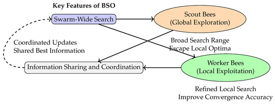
Figure 1.
Illustration of the search mechanism in BSO.
While BSO’s multi-agent search, coordinated information sharing, and dynamic updating mechanisms excel at improving sample diversity and escaping local modes [26], traditional MH algorithms often struggle with these challenges due to their reliance on local proposals and single-chain exploration. Embedding BSO-inspired mechanisms into Bayesian sampling frameworks (e.g., MH) therefore not only expands the exploration capability in the state space but also holds promise for enhancing the stability and efficiency of the sampling process.
2.2. Characteristics and Limitations of Classical MH Sampling
The MH algorithm is a classical representative of MCMC methods that is widely used in Bayesian inference and probabilistic modeling. Its fundamental idea is to construct candidate samples based on the current state and decide whether to accept them according to an acceptance probability, thereby forming a Markov chain that converges to the target distribution.
However, in practical applications, the efficiency of MH is constrained by several factors. First, MH is inherently a local sampling strategy: candidate generation depends on the current state, lacking the ability to perform large jumps across the state space. This makes it prone to getting trapped in local modes, especially in multimodal or high-dimensional distributions, resulting in strong sample autocorrelation and slow convergence. Second, the form of the proposal distribution and the choice of step-size parameters critically affect performance—poorly chosen values can lead to unacceptably low acceptance rates or insufficient exploration. Moreover, MH lacks built-in adaptive adjustment mechanisms and information-sharing capabilities, making it difficult to dynamically optimize sampling trajectories and posing clear disadvantages when dealing with complex posterior structures.
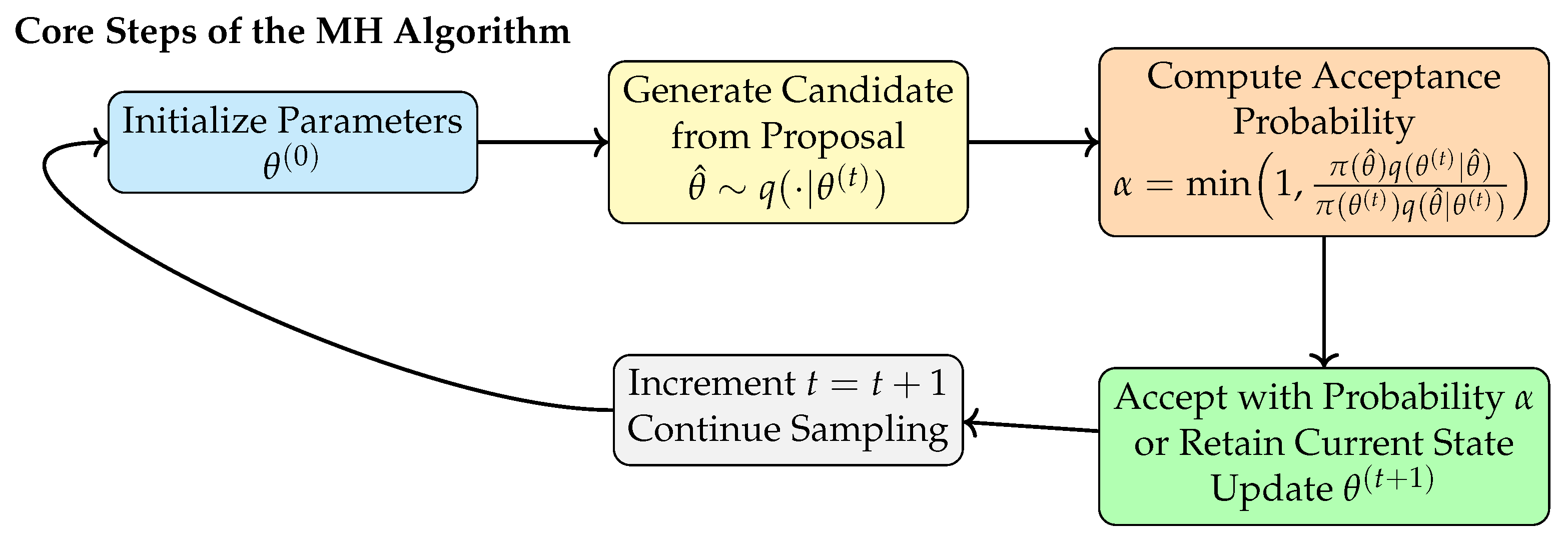
Figure 2 illustrates the standard workflow of the MH algorithm, including initialization, candidate generation, acceptance probability computation, state updates, and iterative sampling. Although the MH procedure is conceptually straightforward, it lacks mechanisms for integrating and coordinating information across samples.
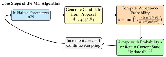
Figure 2.
Workflow of the classical MH algorithm.
Given these limitations, incorporating bee swarm–inspired mechanisms that offer parallel search, information sharing, and dynamic adjustment capabilities has the potential to retain the theoretical strengths of MH while significantly enhancing its ability to efficiently explore complex posterior landscapes. Motivated by this, the present work proposes a hybrid sampling algorithm that integrates swarm intelligence with the MH framework, aiming to balance sampling quality with global exploration capability and to build a more robust and adaptive tool for Bayesian inference.
3. The Proposed BeeSwarm-MH Algorithm
To facilitate the detailed description and implementation of the proposed BeeSwarm-MH algorithm, we first introduce the main variables, control parameters, and convergence diagnostics through a set of well-organized tables. These tables are categorized by function to clearly present the sampling variables, control and adaptation parameters, and statistical indicators used for monitoring convergence.
Table 1 summarizes the core variables involved in the sampling process. Next, Table 2 lists the main control parameters and adaptation factors of the algorithm.

Table 1.
BeeSwarm-MH sampling variables.

Table 2.
BeeSwarm-MH control parameters.
Building on the sampling process and parameter adaptation mechanisms, BeeSwarm-MH also includes a convergence diagnostic module. Table 3 defines the key statistical indicators and thresholds used for convergence assessment.

Table 3.
BeeSwarm-MH statistical indicators and diagnostics.
These symbols and parameter definitions establish a unified and clear notation system for describing the subsequent algorithmic procedures, module designs, and experimental implementation.
3.1. Hybrid Sampling Framework Integrating Bee Swarm Intelligence with MH
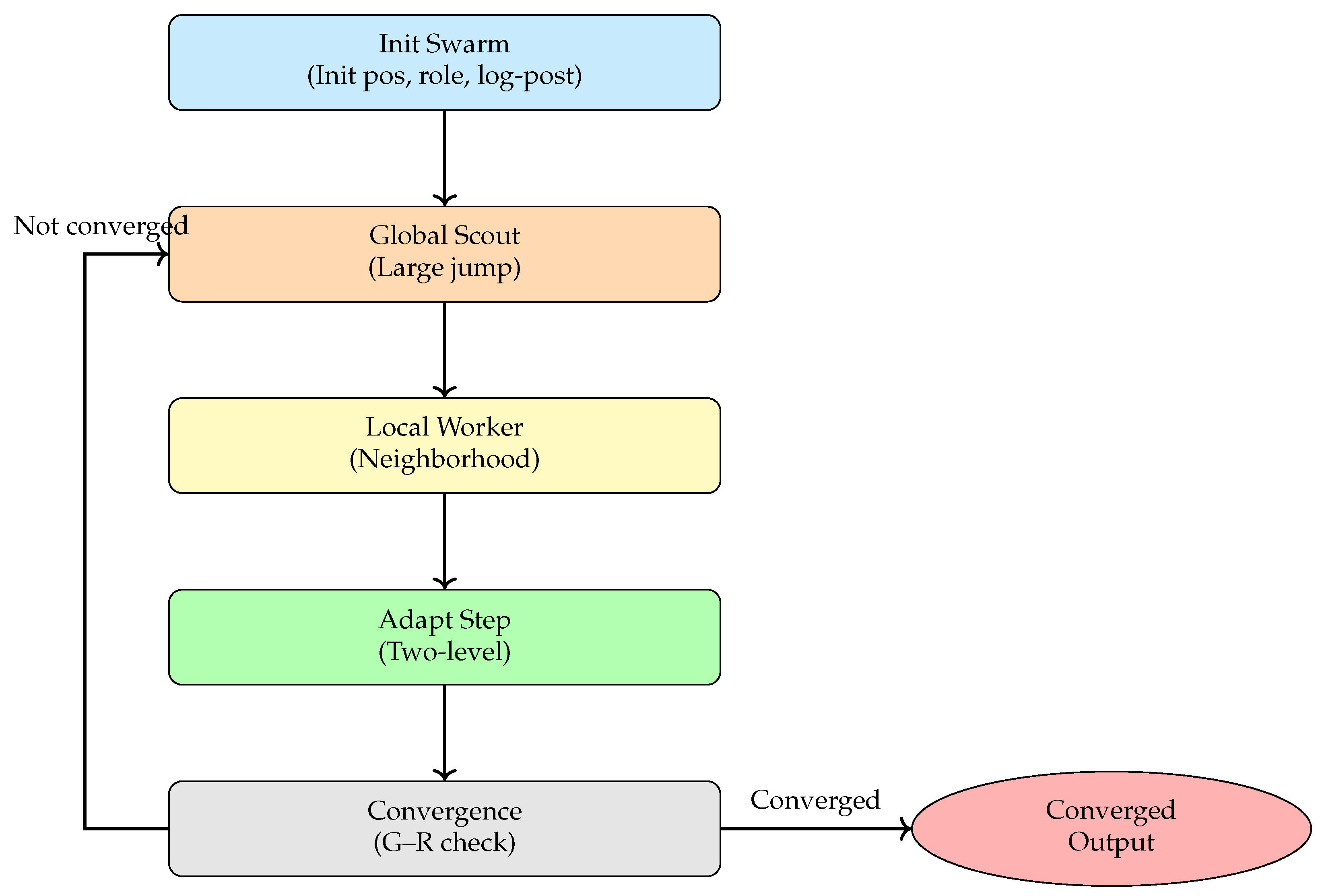
The BeeSwarm-MH algorithm introduces a role-based division of labor inspired by bee swarm intelligence, where scout bees perform global exploration while worker bees focus on local exploitation. By combining this division with the statistical consistency and acceptance rules of MH sampling, the algorithm establishes a framework that balances exploratory jumps with stable local refinement. This design enables a dynamic, adaptive balance between exploration and exploitation in high-dimensional posterior spaces, significantly enhancing the performance of classical MH methods on complex models. The overall workflow is illustrated in Figure 3, which comprises five main modules: bee swarm initialization, global exploration by scout bees, local exploitation by worker bees, adaptive step-size adjustment, and convergence diagnostics with result recording.

Figure 3.
Workflow of the BeeSwarm-MH algorithm.
Figure 3 illustrates the overall workflow of the proposed BeeSwarm-MH sampling algorithm. The process begins with the bee swarm initialization module, which generates the initial set of candidate solutions, assigns roles (scouts and workers), and evaluates their log-posterior probabilities to provide the foundation for subsequent iterative updates. The algorithm then alternates between two complementary search strategies: global exploration by scout bees and local exploitation by worker bees. Scout bees perform large-scale jumps in the parameter space, effectively expanding the search domain and avoiding entrapment in local optima. Worker bees refine promising regions by performing localized perturbations, thereby enhancing local convergence.
On top of this division of labor, the algorithm features an adaptive step-size adjustment mechanism that dynamically updates individual and global proposal scales based on sampling feedback. This ensures a balanced trade-off between exploration and exploitation, improving overall sampling efficiency and stability. After each iteration, a convergence diagnostic based on the Gelman–Rubin statistic evaluates the stability and convergence of the multi-chain sampling process. If the convergence criterion is satisfied, the algorithm terminates and outputs the final posterior samples and parameter estimates; otherwise, it returns to the global exploration stage for continued sampling.
This workflow effectively combines the cooperative search advantages of bee swarm intelligence with the statistical rigor of MH sampling, substantially improving the ability to sample from complex posterior distributions in Bayesian models while maintaining high sample quality. In the following sections, we describe in detail the role allocation in the bee swarm, the search strategies of scout and worker bees, the adaptive step-size mechanism, and the convergence diagnostics employed in the BeeSwarm-MH algorithm.
3.1.1. Bee Swarm Initialization
The bee swarm initialization stage serves as the starting point of the BeeSwarm-MH sampling algorithm, laying the foundation for subsequent global exploration and local exploitation while also defining essential control parameters. First, given the parameter space dimension d, the algorithm allocates a sample trajectory matrix in advance to store the best sample from each iteration. Each individual i in the swarm is then randomly initialized with a parameter vector , and its corresponding log-posterior value is computed as . The local step-size parameter is set to the initial value .
To enable the division of labor within the swarm, the algorithm assigns the first individuals as scout bees (scout) for global exploration, while the remaining individuals become worker bees (worker) responsible for local exploitation, which are marked with the role label . The global covariance matrix is initialized as to define the scale of multidimensional Gaussian perturbations, and the global scaling factor c is set to 1.0 as the baseline for subsequent adaptive step-size adjustment.
In addition, the algorithm defines stage thresholds and to control the multi-phase adjustment of perturbation intensity, implementing an annealing schedule from coarse to fine sampling. The initial mean log-posterior value of the swarm
serves as a baseline reference for later convergence diagnostics. The final output of this step includes the complete swarm state set
and the global control parameter set
which together provide the necessary input for the global exploration, local exploitation, adaptive step-size adjustment, and convergence diagnostics modules of the BeeSwarm-MH algorithm. The detailed initialization procedure is given in Algorithm 1.
| Algorithm 1 Bee Swarm Initialization |
|
Bee swarm initialization establishes the structural and parameter foundations necessary for subsequent stages of the algorithm. Once initialization is complete, the algorithm proceeds to the critical search phase in which scout bees perform global exploration while worker bees focus on local exploitation. The next section details the global exploration strategy of the scout bees, which perform broad searches across the parameter space to help identify promising regions.
3.1.2. Global Exploration by Scout Bees
The global exploration module for scout bees is a critical component of the BeeSwarm-MH sampling algorithm, which is designed to ensure comprehensive coverage of the parameter space by applying staged random perturbations. This mechanism prevents the algorithm from getting trapped in local modes and maintains both sampling diversity and global search capability. Specifically, the algorithm adaptively adjusts the perturbation intensity factor based on the current iteration number t and the predefined stage thresholds and . This phased strategy enables the algorithm to use larger step sizes in early iterations for broad exploration, gradually reducing the step size in later stages to focus on the fine-grained exploitation of promising regions, thus balancing exploration and convergence.
For all individuals labeled as scout bees (scout), the algorithm implements an MH sampling step using a multivariate normal proposal distribution. Each scout bee uses its current position as the mean and generates a new candidate parameter from a scaled covariance matrix , where . The log-posterior of the candidate point is then evaluated as
The acceptance probability is computed according to the MH criterion:
where is the current log-posterior value. A uniform random variable is sampled, and if , the candidate point is accepted, updating the scout’s position and posterior; otherwise, the current position remains unchanged. This procedure guarantees the detailed balance condition and preserves the correctness of the target posterior distribution.
Through this parallel execution of randomized perturbations and acceptance steps, the scout bee module effectively maintains the diversity and stochasticity of the swarm sampling process, providing rich and promising starting points for the subsequent local exploitation phase driven by worker bees. The worker bees capitalize on the prior information identified by scouts to perform high-density local sampling and refined search, achieving a coordinated evolution from global coarse positioning to local fine optimization that significantly improves the efficiency and accuracy of inference in complex Bayesian posteriors. The complete procedure is detailed in Algorithm 2.
| Algorithm 2 Global Exploration by Scouts |
|
After scout bees identify high-potential regions in the parameter space, the algorithm transitions to the local exploitation phase led by worker bees. Worker bees use the prior information provided by scouts to conduct high-density sampling and fine-grained local search, enabling a collaborative evolution from global coarse exploration to local optimization and significantly enhancing the algorithm’s ability to infer complex posteriors with high accuracy.
3.1.3. Local Exploitation by Worker Bees
The local exploitation module for worker bees in the BeeSwarm-MH sampling framework is responsible for the fine-grained exploration of high-potential regions, mimicking the collective foraging behavior of bees around a food source to achieve efficient sampling of local modes in the posterior distribution. This module adaptively selects the local perturbation intensity factor based on the current iteration t and the stage thresholds and . This phased approach ensures that early iterations maintain larger perturbations to avoid premature convergence, while later stages focus on the precise local exploitation of promising regions.
The core mechanism is based on information sharing and probabilistic leadership. The algorithm constructs an exponential-weighted distribution over all individuals’ log-posterior values:
and samples a leader index ℓ from this distribution. This strategy is analogous to a pheromone mechanism, preferentially selecting high-posterior individuals as leaders to strengthen the exploitation of high-fitness regions.
For each worker bee, a multivariate normal proposal distribution is defined around the leader’s position with covariance , from which a candidate solution is drawn. The log-posterior at the proposal is evaluated as and compared with the current value using the MH acceptance probability:
A uniform random variable is then sampled, and the proposal is accepted if , updating the bee’s position and posterior value.
This collaborative exploitation mechanism significantly increases the sampling density and statistical efficiency in local optimum regions. Combined with the staged perturbation adjustment, the module adapts to different phases of sampling convergence, achieving balanced and efficient local sampling in multimodal, complex posterior distributions. The detailed procedure is presented in Algorithm 3.
| Algorithm 3 Local Exploitation by Workers |
|
The worker bee local exploitation strategy enables a fine-grained search around high-potential regions, substantially improving the algorithm’s ability to approximate optimal solutions. Given the dynamic nature of the search landscape, fixed step sizes struggle to balance exploration and exploitation; therefore, an adaptive step-size adjustment mechanism is introduced to dynamically optimize the search scale, further enhancing the convergence efficiency and optimization performance.
3.1.4. Adaptive Step Size Adjustment
The adaptive step-size adjustment module is a critical component of the BeeSwarm-MH sampling algorithm, which is designed to dynamically balance exploration and exploitation while enhancing overall sampling efficiency and robustness. This module implements a two-level strategy, enabling both individual-level adaptation and the global coordination of step sizes.
At the individual level, each bee tracks its proposal count and acceptance count. Once the number of proposals exceeds the threshold , the local acceptance rate is computed as
Drawing on the adaptive sampling principle of balancing exploration and exploitation in MCMC methods [12], a local adjustment factor is then calculated:
This coefficient (0.2) is determined through empirical tuning specific to the BeeSwarm-MH framework, ensuring the appropriate responsiveness of individual step sizes to local acceptance rate variations. This function ensures that when acceptance rates are high, the step size is moderately increased to expand the search range; conversely, when acceptance rates are low, the step size is reduced to improve sampling success. The updated step size is clipped within a predefined range using
to prevent numerical instability or degradation. After adjustment, the proposal and acceptance counters are reset for the next cycle.
At the global level, the module computes the overall acceptance rate across the swarm:
Following the same adaptive logic inspired by [12] and optimized for swarm coordination, it uses this rate to evaluate the global scaling adjustment function:
The smaller coefficient (0.1) here is tailored to maintain stable swarm-level coordination while still enabling collective adaptation to the global sampling landscape. The global scaling factor c is updated accordingly and clipped within the range
Subsequently, all individual step sizes are multiplied by this updated global scaling factor, achieving coordinated adjustment across the entire swarm.
In summary, this two-level step-size adjustment mechanism leverages individual feedback and collective coordination to prevent step-size degeneration and premature convergence, thereby significantly improving the algorithm’s adaptability and sampling quality in complex parameter spaces. The full procedure is detailed in Algorithm 4.
| Algorithm 4 Adaptive Step Size Adjustment |
|
This adaptive step-size adjustment mechanism effectively improves sampling efficiency and convergence stability. To further ensure the reliability of the algorithm’s output, the next section introduces a convergence diagnostic module, which enables the automatic detection of stable states, enforces clear stopping criteria, and optimizes the use of computational resources.
3.1.5. Convergence Diagnosis and Results Output
The convergence diagnosis module provides a clear and automated criterion for assessing the convergence of the BeeSwarm-MH sampling process while standardizing the recording of the best samples at each iteration. This ensures the sufficient exploration of the posterior space and avoids unnecessary computational overhead.
At each iteration t, the algorithm computes the maximum log-posterior value among all swarm individuals:
and appends it to the historical best-value sequence
which characterizes the temporal evolution of the global optimal posterior and is used to monitor the convergence trend.
Once the iteration count exceeds the sliding window length W, the variance of the latest W best values is calculated:
If this variance satisfies
the sampling process is considered converged, indicating that the optimal posterior value has stabilized and the swarm search has reached a steady state. This criterion, based on the stationarity of the best-value sequence, is straightforward and computationally efficient, making it especially suitable for complex multimodal posterior distributions where traditional diagnostics such as the Gelman–Rubin statistic may be difficult to apply.
Simultaneously, the algorithm records the parameter vector of the current best individual at each iteration:
forming a time-series sample matrix (with columns corresponding to time steps):
which serves as the data foundation for subsequent Bayesian parameter estimation and uncertainty quantification. The detailed procedure is summarized in Algorithm 5.
| Algorithm 5 Convergence Diagnosis and Results Output |
|
Following the completion of core modules such as adaptive step-size adjustment and convergence diagnosis, these components will be integrated to construct the complete BeeSwarm-MH main procedure, enabling efficient closed-loop control from initialization to convergence output.
3.2. BeeSwarm-MH Main Procedure
Based on the organic integration of the scout bee global exploration, worker bee local exploitation, adaptive step-size adjustment, and convergence diagnosis modules introduced above, the complete BeeSwarm-MH main procedure is constructed in Algorithm 6. This workflow systematically drives efficient iterations of the algorithm, enabling accurate Bayesian inference within complex parameter spaces.
This BeeSwarm-MH main procedure provides an efficient and stable sampling scheme for complex Bayesian inference problems. The following section demonstrates the application and performance of the algorithm in Bayesian parameter estimation for the Ginzburg–Landau equation based on this workflow.
| Algorithm 6 BeeSwarm-MH Main Procedure |
|
4. Bayesian Inference for the Ginzburg–Landau Equation
To validate the applicability of the BeeSwarm-MH sampling algorithm in Bayesian inference, we perform parameter estimation for the complex Ginzburg–Landau (GL) equation using both the BeeSwarm-MH sampling and the classical MH sampling. For clarity, we restrict the comparison to these two methods; Adaptive MH and HMC were omitted because their gradient and tuning overheads are prohibitive for the present forward model.
All computations were conducted in a Python 3.9 environment, utilizing essential libraries such as Matplotlib 3.8.4, NumPy 1.26.4, Pandas 2.2.3, and SciPy 1.13.0. Simulations were performed on a personal laptop equipped with an Intel Core i9 processor and 32 GB of RAM.
4.1. The GL Equation and Its Soliton Solution
Consider the complex GL equation with initial and boundary conditions as presented in [27]:
where the system can be viewed as a controllable optical pulse model:
By adjusting the parameters , , and , we can simulate the propagation of optical pulses in mode-locked lasers, thereby studying the evolution of spatiotemporal dissipative optical solitons. Here, denotes the group velocity dispersion coefficient, which influences pulse broadening; is the third-order nonlinear coefficient related to self-phase modulation effects; and represents the gain coefficient of the amplifying fiber.
Particularly, when the selected optical parameters balance dispersion, fiber nonlinearity, laser gain saturation, and gain bandwidth filtering effects, the governing equation (1) admits an exact solution [27]. Define
Then, Equation (1) has the analytical solution
In particular, for the parameter set , the soliton solution profile at time is illustrated in Figure 4.
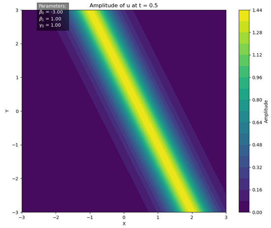
Figure 4.
Soliton solution of the GL equation at .
Given observed data , we employ the BeeSwarm-MH sampling method to infer the parameters .
4.2. Preparation of Observed Data
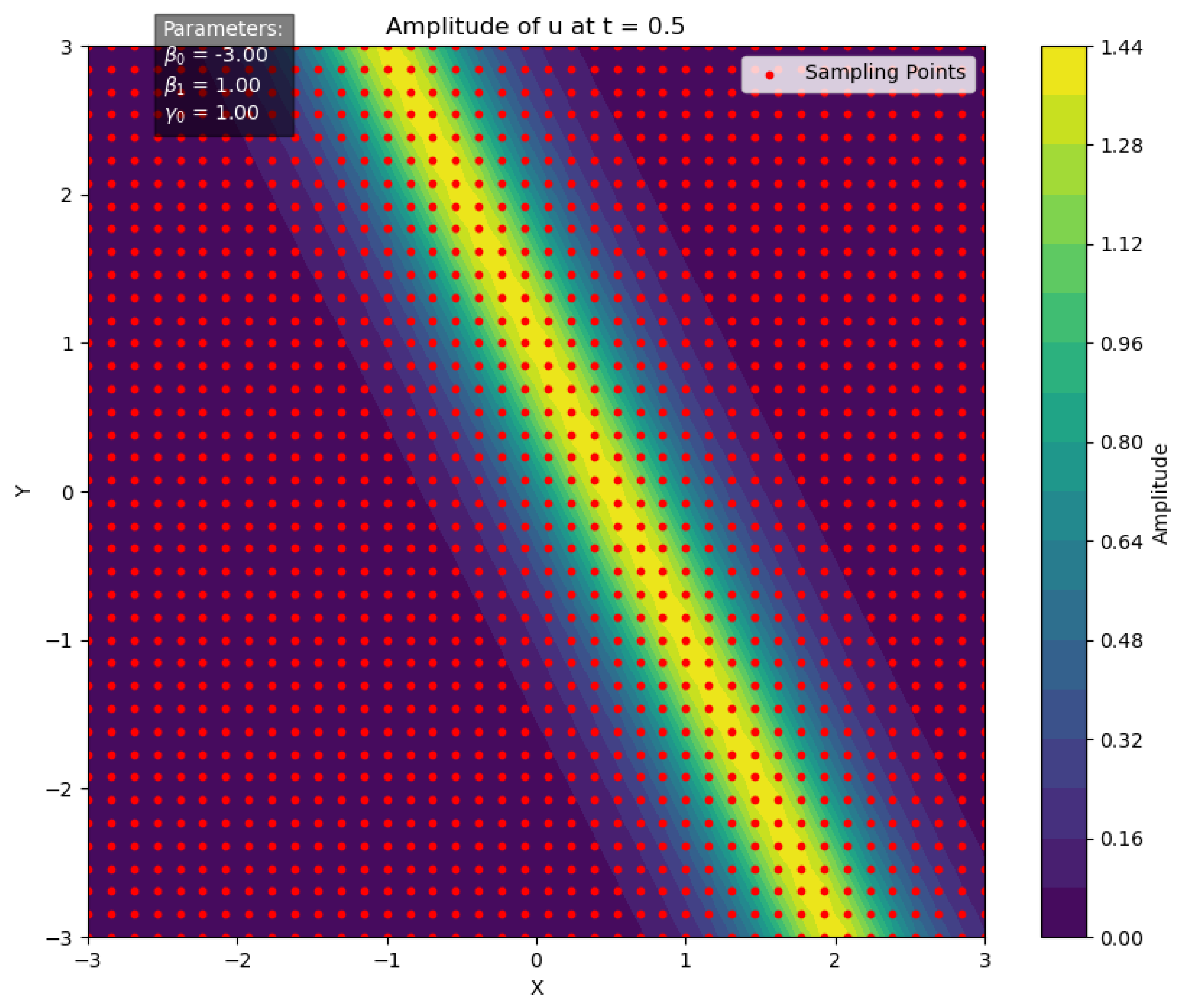
At time , with parameters set as , the two-dimensional spatial domain is uniformly sampled to generate a grid of points , totaling data points, as illustrated in Figure 5. For each grid point, the function value is computed, and random perturbations are applied to obtain the perturbed values :
where represents random noise drawn from a specified distribution.

Figure 5.
Initial sampling points for Bayesian inference.
4.3. Bayesian Inference Algorithm Based on Sampling Strategies
After obtaining the observed data , we perform Bayesian inference on the three parameters of the GL equation. Below, we introduce the prior distribution, likelihood function, and posterior distribution involved in the Bayesian inference.
In Bayesian inference, the prior distribution reflects prior knowledge of the parameters before observing data. For the GL equation parameters , we assume uniform prior distributions over the ranges , , and , respectively. Specifically, we use uniform (log-constant) priors whose logarithmic probability is given by
The likelihood function quantifies the probability of the observed data given the model parameters, facilitating the computation of the posterior distribution. The log-likelihood is defined as
where denotes the perturbed observed amplitude at the i-th observation point, and is the model-predicted amplitude at that point. Here, is the standard deviation of the noise, and N is the total number of observations.
The posterior distribution combines prior knowledge and observed data, providing a comprehensive description of the model parameters for estimation and uncertainty quantification. Its logarithm is given by the sum of the log-likelihood and the log-prior:
To compare the performance of different sampling strategies in Bayesian parameter estimation, we design a unified framework compatible with both the classical MH and the BeeSwarm-MH methods incorporating swarm intelligence. Algorithm 7 presents the pseudocode of this general sampling procedure, which flexibly switches between sampling mechanisms according to the selected strategy, performing adaptive optimization and convergence assessment at each iteration.
| Algorithm 7 Bayesian Parameter Estimation Framework Based on Sampling Strategies |
|
After establishing the Bayesian inference framework and implementing both the BeeSwarm-MH and classical MH sampling strategies, the following section validates the performance of these algorithms through numerical experiments. We compare their accuracy, efficiency, and robustness in estimating the parameters of the GL equation.
4.4. Convergence Diagnostics
To ensure the robustness and reliability of our Bayesian inference results, we employed two primary statistical diagnostics: the sliding-window variance and the Gelman–Rubin test.
- Sliding-Window Variance: The sliding-window variance v is calculated over the last W iterations of the log-posterior values . This variance is used to monitor the stability of the sampling process. Specifically, we compute v aswhere is the maximum log-posterior value at iteration t. If v falls below a predefined threshold , it indicates that the sampling process has stabilized.
- Gelman–Rubin Test: The Gelman–Rubin test assesses convergence by comparing the within-chain and between-chain variances. We initialize four independent chains with different starting points and compute the potential scale reduction factor (PSRF) R. The PSRF is defined aswhere is the estimated variance of the target distribution and W is the within-chain variance. Convergence is achieved when .
These diagnostics are implemented in Algorithm 5, where we detail the steps for computing and applying these tests to determine convergence.
4.5. Experimental Setup
The key hyperparameters used in the BeeSwarm-MH algorithm are summarized in Table 4. This table provides a comprehensive overview of the parameter settings that were used throughout the experiments.

Table 4.
Hyperparameter values for BeeSwarm-MH algorithm.
In addition to the hyperparameters listed in the table, the initial parameters were set to , and the covariance matrix was initialized as a diagonal matrix with as the diagonal elements. The bee roles were assigned such that 50% of the bees were scouts and 50% were workers.
4.6. Experimental Results and Analysis for BeeSwarm-MH Inference
Based on the Bayesian inference framework utilizing the BeeSwarm-MH sampling, we conduct an in-depth study of the method’s performance and statistical significance in parameter estimation through both graphical visualization and algorithmic analysis.
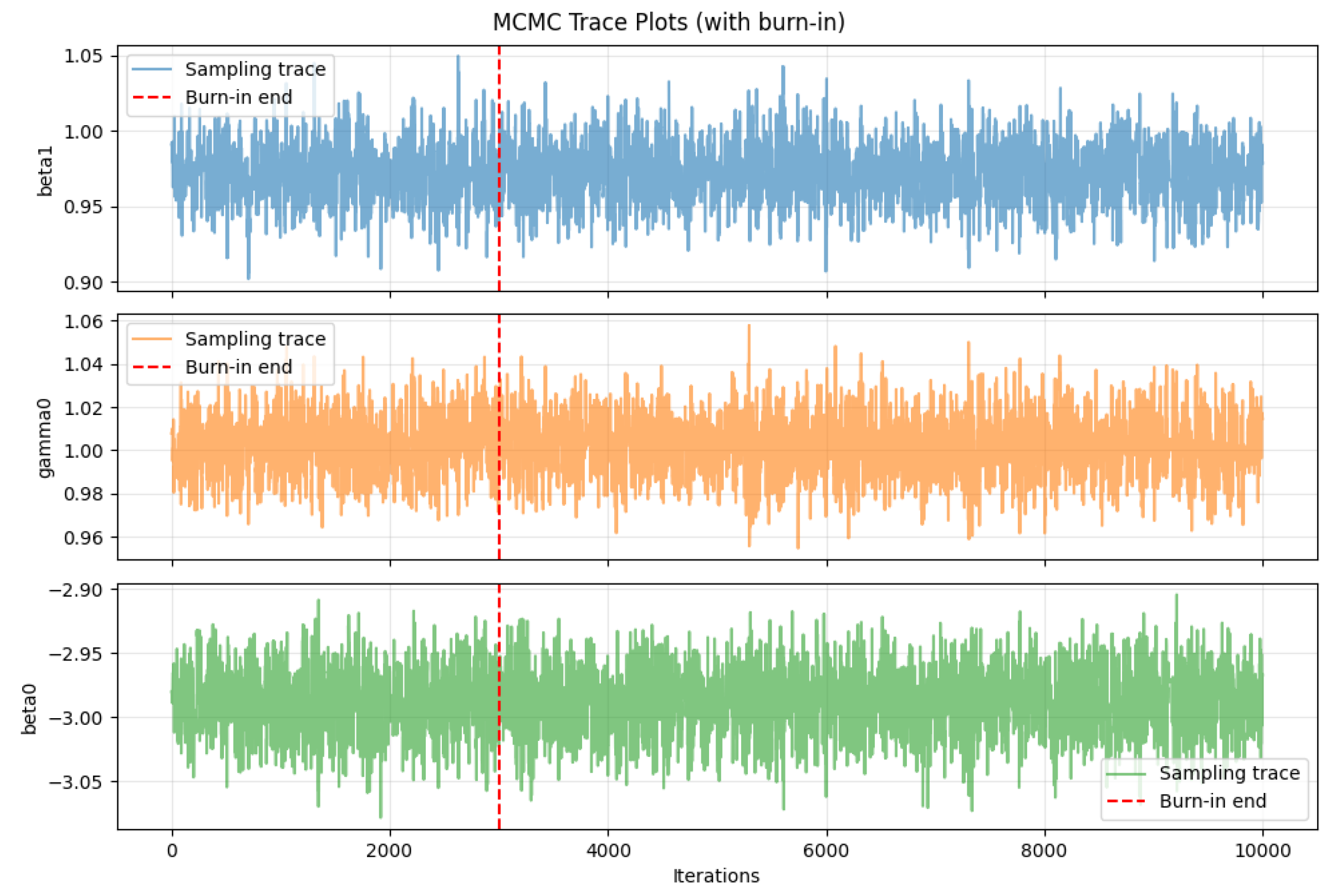
Figure 6 shows the MCMC trace plots for the parameters , , and , where the red dashed lines indicate the burn-in cutoff. It can be observed that all three chains rapidly enter a stable fluctuation region after burn-in, exhibiting no apparent systematic drift or significant trending behavior. This indicates that the Markov chains have successfully converged to the target posterior distributions and demonstrate good mixing properties. The sampling traces maintain an approximately stable mean level amidst high-frequency oscillations, further confirming adequate exploration of the parameter space and providing a reliable foundation for posterior statistical inference.
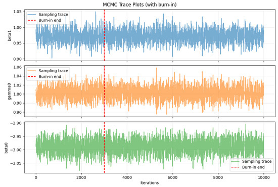
Figure 6.
MCMC trace plots for BeeSwarm-MH sampling.
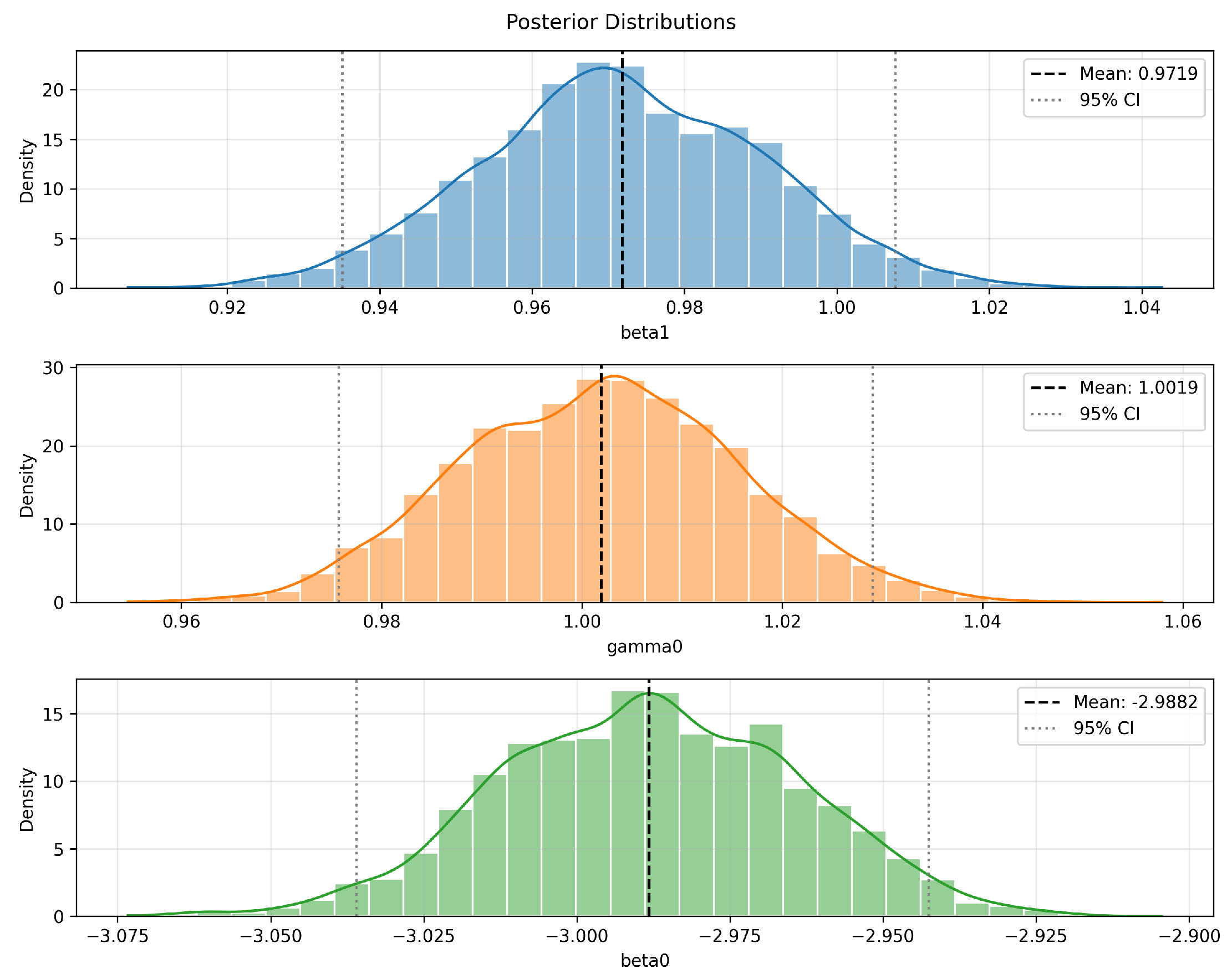
Figure 7 presents the marginal posterior distributions of the corresponding parameters. All parameters exhibit unimodal characteristics: appears approximately symmetric, shows slight right skewness, and displays slight left skewness. The black dashed lines represent the posterior means, while the gray dashed lines denote the 95% posterior credible intervals, illustrating the concentration of estimates and uncertainty bounds. Overall, the posterior distributions are smooth with well-defined mean estimates, reflecting strong parameter identifiability given the observed data and demonstrating the robustness and statistical reliability of the posterior inference.

Figure 7.
Posterior distributions of GL-equation parameters obtained via BeeSwarm-MH.
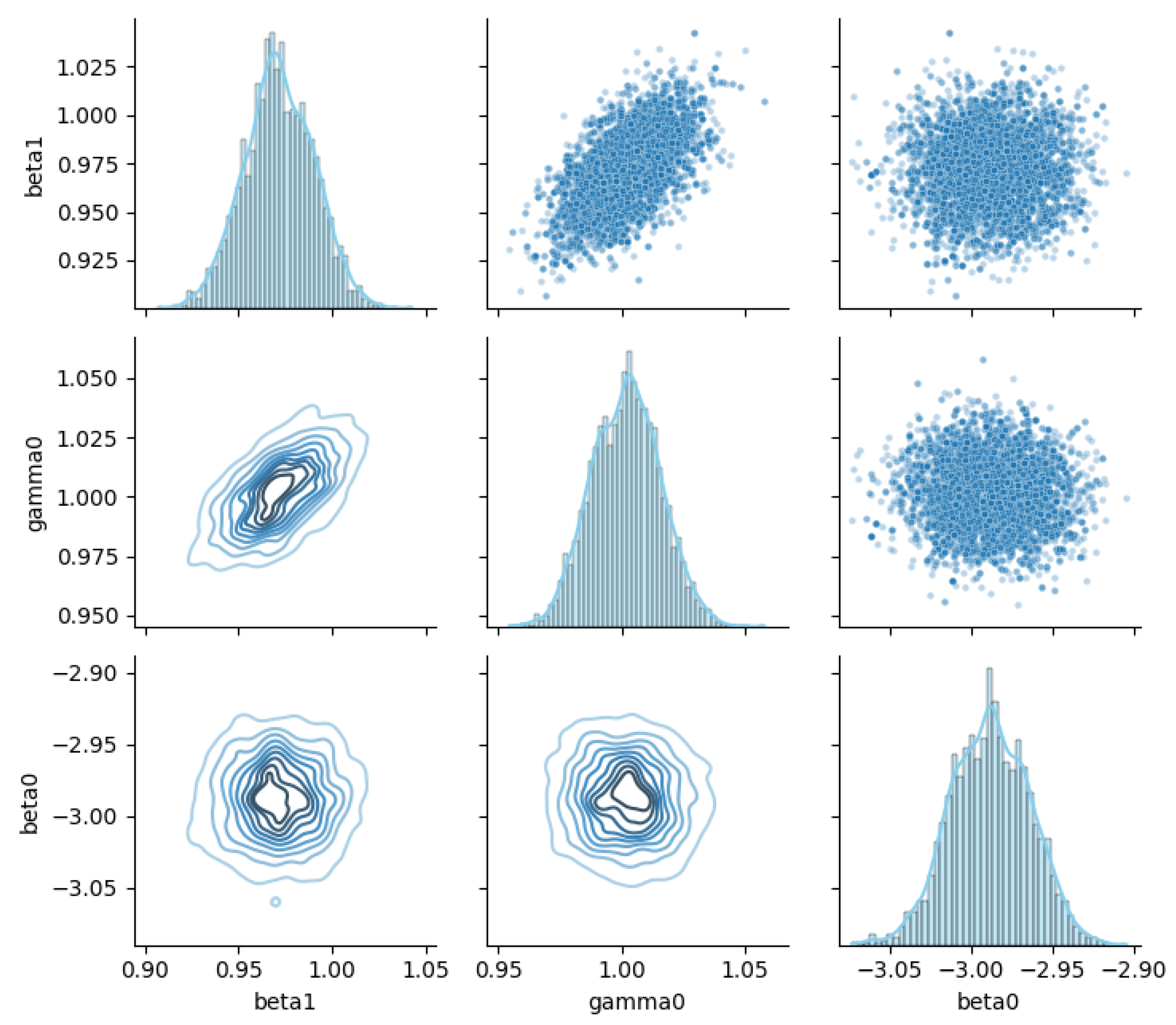
Figure 8 depicts the joint posterior relationship matrix for the parameters , , and . This figure provides a multidimensional characterization of parameter dependencies via univariate marginal distributions on the diagonal, scatter plots above the diagonal, and kernel density contour plots below the diagonal.
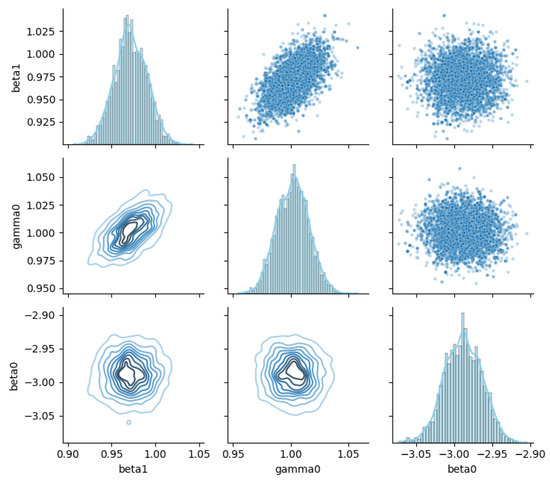
Figure 8.
Joint posterior relationships among GL-equation parameters.
On the diagonal, both and display unimodal, concentrated distributions, while exhibits a clear peak with well-defined intervals, indicating robust univariate posterior estimates. The upper-triangular scatter plots reveal a weak positive correlation clustering trend between and , whereas other variable pairs show more dispersed relationships, exposing complex dependence structures. The lower-triangular contour plots further confirm that the joint distribution of and is concentrated along a specific direction, while shows multimodal local clustering with the other two parameters, highlighting nontrivial nonlinear associations.
Table 5 reports the parameter-specific posterior means and the overall Gelman–Rubin statistic computed from four independent MCMC chains after 10,000 iterations (burn-in 3000). All three parameters achieve , confirming adequate convergence.

Table 5.
Gelman–Rubin diagnostics after 10,000 iterations (4 chains, burn-in 3000).
Figure 9 displays the post-burn-in trace plots (left) and the corresponding chain-wise Gelman–Rubin statistics (right) for the three model parameters , , and . Four independent MCMC chains are plotted in distinct colors with dashed horizontal lines indicating the overall posterior mean for each parameter. The red dashed line at marks the convergence threshold, and all computed values lie below this limit, confirming adequate mixing across the four chains.
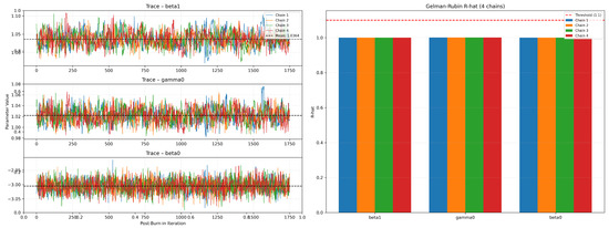
Figure 9.
Gelman—Rubin diagnostics 4 chains per parameter.
In summary, the posterior parameter distributions combine concentrated univariate behavior with intricate multivariate dependencies, reflecting both effective constraint on core parameters and rich exploration of the parameter space. This provides key insights for an in-depth analysis of model fit and structural characteristics, underpinning the statistical credibility and robustness of the subsequent Bayesian inference.
4.7. Algorithm Performance Comparison
We systematically compare the performance of the BeeSwarm-MH sampling method and the classical MH approach for Bayesian inference of the GL equation parameters from three perspectives: computational efficiency, sampling quality, and algorithmic characteristics.
4.7.1. Computational Time
Table 6 summarizes the runtime performance of the classical MH algorithm and the BeeSwarm-MH algorithm. The results indicate that BeeSwarm-MH achieves a significant advantage in computational efficiency, reducing the total runtime to 34.7% of that of the classical MH (76.18 s vs. 219.47 s). This improvement primarily stems from its early convergence feature, requiring only iterations to reach convergence compared to the full iterations in the classical MH. Notably, the post-processing time of BeeSwarm-MH accounts for only 17.1% of that of the classical MH ( s vs. s), which can be attributed to its dynamic sample filtering and adaptive convergence diagnostics.

Table 6.
Performance comparison between classical MH and BeeSwarm-MH.
4.7.2. Sampling Quality and Parameter Estimation
Table 7 compares the sampling quality and parameter estimation results of the two algorithms. Although the effective sample size (ESS) of BeeSwarm-MH is slightly lower than that of the classical MH for certain parameters (e.g., ESS for is 1451 vs. 2447), the acceptance rates ( vs. ) and R-hat convergence diagnostics (all below ) are comparable, indicating satisfactory sample quality for statistical inference. Parameter estimates also show high agreement between the two methods with nearly identical posterior means and 95% credible intervals—for instance, estimated at (MH) and (BeeSwarm-MH), with negligible differences.

Table 7.
Comparison of sampling quality and parameter estimates.
4.7.3. Algorithmic Characteristics and Applicability
BeeSwarm-MH employs a swarm cooperation mechanism to dynamically balance global exploration and local exploitation. Its adaptive step size adjustment and structured bee roles (scout and worker bees) provide greater robustness in complex parameter spaces. In contrast, the classical MH algorithm relies on a random-walk mechanism that is prone to local trapping in high-dimensional or multimodal distributions. A summary of key algorithmic characteristics and their respective suitable application scenarios is provided in Table 8.

Table 8.
Comparison of algorithmic characteristics and applicability.
4.7.4. Summary of Algorithm Comparison
The experimental results demonstrate that BeeSwarm-MH achieves nearly a threefold improvement in computational efficiency while maintaining parameter estimation accuracy comparable to the classical MH algorithm. Its enhanced automation and global optimization capabilities make it a superior choice for complex Bayesian inference tasks, especially when computational resources are limited or the parameter space exhibits unknown multimodality.
5. Conclusions and Future Work
In this study, we proposed the BeeSwarm-MH algorithm, which integrates BSO with the MH acceptance criterion, effectively overcoming the limitations of traditional Bayesian inference sampling methods. In parameter estimation experiments for the GL equation, the proposed algorithm reduced runtime by 65.3% compared to the classical MH method, achieving convergence with only 10% of the iterations required by MH. Key parameter estimation biases were below 0.001, and all R-hat convergence diagnostics were below 1.0014, satisfying Bayesian inference convergence criteria.
The core innovation of the algorithm lies in the novel integration of BSO-inspired scout–worker bee division of labor with the MH acceptance mechanism, which is supplemented by a two-level adaptive step size adjustment strategy. This design achieves a dynamic balance between global exploration and local exploitation, addressing the sensitivity of classical MH algorithms to step size selection.
Future work will focus on three main directions: extending the algorithm’s applicability to high-dimensional parameter spaces by enhancing parallel computing efficiency; conducting an in-depth theoretical analysis of convergence rates and ergodicity under multimodal target distributions; and applying the algorithm to complex physical systems, biomedical modeling, and real-time inference scenarios. Specifically, we will pursue GPU-accelerated implementations, derive spectral-gap bounds via weak-Poincaré techniques, and release an open-source Python package for real-world deployment. Additionally, challenges related to extremely multimodal distributions and strong parameter dependencies warrant further investigation to improve robustness and scalability.
Author Contributions
Conceptualization, S.X. and L.Z.; methodology, L.Z.; software, L.Z.; validation, S.X.; formal analysis, L.Z.; investigation, S.X.; resources, S.X. and L.Z.; writing—original draft preparation, S.X.; writing—review and editing, L.Z.; visualization, S.X.; supervision, L.Z.; project administration, L.Z.; funding acquisition, S.X. and L.Z. All authors have read and agreed to the published version of the manuscript.
Funding
Supported by the Open Fund of Zhejiang Key Laboratory of Film and TV Media Technology, No. 2024E10023.
Data Availability Statement
All code and data used in this study are publicly available at https://figshare.com/articles/dataset/BeeSwarm-MH_Sampling_for_Bayesian_Inference_of_GL_Equation_Parameters/29345459 (accessed on 31 July 2025).
Conflicts of Interest
The authors declare no conflicts of interest.
References
- Metropolis, N.; Rosenbluth, A.W.; Rosenbluth, M.N.; Teller, A.H.; Teller, E. Equation of state calculations by fast computing machines. J. Chem. Phys. 1953, 21, 1087–1092. [Google Scholar] [CrossRef]
- Hastings, W.K. Monte Carlo sampling methods using Markov chains and their applications. Biometrika 1970, 57, 97–109. [Google Scholar] [CrossRef]
- Brooks, S.; Gelman, A.; Jones, G.; Meng, X.-L. (Eds.) Handbook of Markov Chain Monte Carlo; CRC Press: Boca Raton, FL, USA, 2011. [Google Scholar]
- Neal, R.M. MCMC using Hamiltonian dynamics. In Handbook of Markov Chain Monte Carlo; Brooks, S., Gelman, A., Jones, G.L., Meng, X.-L., Eds.; Chapman & Hall/CRC: Boca Raton, FL, USA, 2011. [Google Scholar]
- Andrieu, C.; De Freitas, N.; Doucet, A.; Jordan, M.I. An introduction to MCMC for machine learning. Mach. Learn. 2003, 50, 5–43. [Google Scholar] [CrossRef]
- Taniguchi, T.; Yoshida, Y.; Matsui, Y.; Le Hoang, N.; Taniguchi, A.; Hagiwara, Y. Emergent communication through Metropolis-Hastings naming game with deep generative models. Adv. Robot. 2023, 37, 1266–1282. [Google Scholar] [CrossRef]
- Roberts, G.O.; Rosenthal, J.S. Optimal scaling of Metropolis algorithms: Heading toward general target distributions. Can. J. Stat. 2008, 36, 483–503. [Google Scholar] [CrossRef]
- Andrieu, C.; Lee, A.; Power, S.; Wang, A.Q. Comparison of Markov chains via weak Poincaré inequalities with application to pseudo-marginal MCMC. Ann. Stat. 2022, 50, 3592–3618. [Google Scholar] [CrossRef]
- Roberts, G.O.; Gelman, A.; Gilks, W.R. Weak convergence and optimal scaling of random walk Metropolis algorithms. Ann. Appl. Probab. 1997, 7, 110–120. [Google Scholar] [CrossRef]
- Gelman, A.; Roberts, G.O.; Gilks, W.R. Efficient Metropolis jumping rules. In Bayesian Statistics 5; Oxford University Press: Oxford, UK, 1996; pp. 599–608. [Google Scholar]
- Cowles, M.K.; Carlin, B.P. Markov chain Monte Carlo convergence diagnostics: A comparative review. J. Am. Stat. Assoc. 1996, 91, 883–904. [Google Scholar] [CrossRef]
- Haario, H.; Saksman, E.; Tamminen, J. An adaptive Metropolis algorithm. Bernoulli 2001, 7, 223–242. [Google Scholar] [CrossRef]
- Betancourt, M. A conceptual introduction to Hamiltonian Monte Carlo. arXiv 2017, arXiv:1701.02434. [Google Scholar]
- Geyer, C.J. Markov chain Monte Carlo maximum likelihood. In Proceedings of the 23rd Symposium on the Interface, Seattle, WA, USA, 21–24 April 1991; American Statistical Association: Alexandria, VA, USA, 1991; pp. 156–163. [Google Scholar]
- Earl, D.J.; Deem, M.W. Parallel tempering: Theory, applications, and new perspectives. Phys. Chem. Chem. Phys. 2005, 7, 3910–3916. [Google Scholar] [CrossRef] [PubMed]
- Angelino, E.; Johnson, M.J.; Adams, R.P. Patterns of scalable Bayesian inference. Found. Trends Mach. Learn. 2016, 9, 119–247. [Google Scholar] [CrossRef]
- Pham, D.T.; Ghanbarzadeh, A.; Koc, E.; Otri, S.; Rahim, S.; Zaidi, M. The Bees Algorithm—A Novel Tool for Complex Optimisation Problems. In Proceedings of the 2nd International Virtual Conference on Intelligent Production Machines and Systems, Virtual, 3–14 July 2006; Elsevier: Amsterdam, The Netherlands, 2006; pp. 454–459. [Google Scholar]
- Karaboga, D.; Basturk, B. A powerful and efficient algorithm for numerical function optimization: Artificial bee colony (ABC) algorithm. J. Glob. Optim. 2007, 39, 459–471. [Google Scholar] [CrossRef]
- Akay, B.; Karaboga, D. A modified artificial bee colony algorithm for real-parameter optimization. Inf. Sci. 2012, 192, 120–142. [Google Scholar] [CrossRef]
- Singh, A.; Deep, K. Artificial Bee Colony algorithm with improved search mechanism. Soft Comput. 2019, 23, 12437–12460. [Google Scholar] [CrossRef]
- Nadimi-Shahraki, M.H.; Taghi Valadi, M.; Mirjalili, S. MTV-SCA: Multi-Trial Vector-Based Sine Cosine Algorithm. In Cluster Computing; Springer: Berlin/Heidelberg, Germany, 2024. [Google Scholar]
- Zhang, Y.; Wang, S.; Ji, G. A comprehensive survey on particle swarm optimization algorithm and its applications. Math. Probl. Eng. 2015, 2015, 931256. [Google Scholar] [CrossRef]
- Yang, X.S. Nature-Inspired Metaheuristic Algorithms, 2nd ed.; Luniver Press: Leiden, The Netherlands, 2010. [Google Scholar]
- Pham, D.T.; Ghanbarzadeh, A.; Koc, E.; Otri, S.; Rahim, S.; Zaidi, M. The Bees Algorithm; Technical Note; Manufacturing Engineering Centre, Cardiff University: Cardiff, UK, 2005. [Google Scholar]
- Rey-Bellet, L.; Spiliopoulos, K. Improving the convergence of reversible samplers. J. Stat. Phys. 2016, 164, 472–494. [Google Scholar] [CrossRef]
- Zibaei, H.; Mesgari, M.S. Improved discrete particle swarm optimization using Bee Algorithm and multi-parent crossover method. arXiv 2024, arXiv:2403.10684. [Google Scholar]
- Zhao, Z.; Dai, Z.; Li, D. Breather type of chirped soliton solutions for the 2D Ginzburg–Landau equation. Commun. Nonlinear Sci. Numer. Simul. 2011, 16, 1712–1719. [Google Scholar] [CrossRef]
Disclaimer/Publisher’s Note: The statements, opinions and data contained in all publications are solely those of the individual author(s) and contributor(s) and not of MDPI and/or the editor(s). MDPI and/or the editor(s) disclaim responsibility for any injury to people or property resulting from any ideas, methods, instructions or products referred to in the content. |
© 2025 by the authors. Licensee MDPI, Basel, Switzerland. This article is an open access article distributed under the terms and conditions of the Creative Commons Attribution (CC BY) license (https://creativecommons.org/licenses/by/4.0/).


