Abstract
The reliability and efficiency of power system operations, especially in smart grid scenarios, depend on accurate load demand forecasting. Electrical load forecasting is crucial for power system design, fault protection and diversification as it reduces operating costs while enhancing the system’s overall reliability, stability, and efficiency from an economic and technical perspective. Previously, load forecasting analysis has frequently been limited by inadequate feature engineering and insufficient model tuning. Prediction reliability was reduced by many previous methods’ inabilities to accurately evaluate short-term variations over time and the impact of important variables. These constraints encouraged us to develop a more reliable and thorough forecasting procedure. This research proposes an enhanced short-term load forecasting framework based on a hyperparameter-tuned long short-term memory (LSTM) using a deep learning method recurrent neural network (RNN), alongside more neural network-based models such as artificial neural networks, k-nearest neighbors, and backpropagation neural networks. Hyperparameter optimization techniques (Keras Tuner, Grid SearchCV, Scikeras + Randomized SearchCV, etc.) were used to systematically tune training parameters, learning rates, and network architectures for each forecasting model to increase model accuracy. To provide a more reliable and accurate evaluation of forecasting performance, this research employs the use of an hourly load dataset (2003–2014) enhanced with historical and environmental variables. Significant statistical metrics, such as a mean absolute error of 0.0048, root mean squared error of 0.0091, coefficient of determination of R2 0.9958, and mean absolute percentage error of 1.60%, demonstrate that the hyperparameter optimized with hourly data performed better than both conventional and other deep learning models, with the highest efficiency of all tested models. In accordance with the results, accurate LSTM-RNN parameter modification significantly improves prediction accuracy.
1. Introduction
Electricity plays a pivotal role in everyday life, particularly as the population grows and electricity demand increases. Modern power generation requires an uninterrupted supply of electricity to the load demand [1]. For the purpose of minimizing errors for a continuous power supply, this system requires a precise prediction of both present and future load requirements. To achieve this goal, researchers have been working on creating an effective technique called load forecasting [2]. This process entails predicting future demands for electricity consumption, and is essential to decision-making processes related to fuel allocation, network management, unit commitment, dispatch methods, and other operational areas [3,4]. Electrical load forecasting is growing increasingly crucial in smart grid planning and operation due to the increasing integration of renewable energy sources (RES) into the overall composition of electricity sources and the evolution of the traditional electric grid into a more intelligent, adaptable, and interactive system [5,6,7]. The power system’s safety, dependability, and cost-effective operation depend on accurate multi-node load forecasting. Accurate load forecasting is crucial for maintaining a balance between power supply and demand, as the power generated from RES, including energy storage, linear, and nonlinear loads, varies with weather variables such as wind speed and irradiation which may lead to power quality issues like voltage sag [8]. Utilizing load forecasting, the utility sector can estimate future electrical load demand, reducing the disparity between the demand and generation sides and detect fault locations accurately by comparing actual and short-term forecasted load consumption instantly.
Data on electric load consumption is a time series that includes both linear and nonlinear components and consists of a series of observations made at regular intervals [9]. A mismatch between supply and demand brought on by inflated load requirements may result in grid instability, while minimizing these may result in surplus power generation and market trading. Whether in the distribution system or in individual homes, predicting electric load is difficult because of its high level of variability and unpredictability [10]. For the purpose of predicting future load needs, load forecasting analyzes historical data and patterns of reliance in time-step observations. It has many uses in power system planning and operation, including energy trading, unit commitment, demand response, scheduling, system planning, and energy policy. To balance supply and demand, reduce load shedding-related power outages, and prevent an excess reserve of power generation, energy suppliers and decision makers need precise load forecasting [11]. By utilizing precise forecasts, utilities can plan for optimal load flow, unit commitment, load dispatch, demand response management, and contingency planning, thereby reducing inadequate resource consumption and cost surpluses. Classified as a form of time-series issue requiring expert solutions, load forecasting is a difficult task due to its complexity, unpredictability, and the wide range of factors influencing predictions [12]. Forecasting can be classified as short-term, medium-term, long-term, and very short-term based on the time horizon, as shown in Table 1.

Table 1.
Different types of electrical load forecast [12].
To increase power generation efficiency, load forecasting has drawn the attention of researchers, who have looked into several cutting-edge techniques. The accuracy of these techniques is being hampered by the following issues. The unpredictable nature of weather is one of the crucial obstacles researchers face when creating a load forecasting technique. As for forecasting, load is the dependent variable, depending on weather, temperature, humidity, etc., as these are the independent variables. Both traditional and intelligent metering systems have an effect on load predictions. To prevent forecasting errors, the utility sector must create separate forecasting algorithms for each metering system. Another challenging element that affects the load forecasting model is data collection. The network’s irregularities or unexpected faults must be considered when designing a model. Furthermore, while selecting a forecasting model, the utility company should consider an acceptable margin of error [11,12].
Accurate and effective load forecasting is becoming increasingly critical as the complexity of energy demand increases due to the integration of RES, smart grid, energy storage, etc. This research paper is driven by the need to build a robust and data-driven forecasting framework that addresses current gaps in both modeling and optimization. The main contributions of this study are as follows:
- The long short-term memory—recurrent neural network (LSTM-RNN) forecasting model was developed to enhance long-term dependency learning from historical load data, enabling the capture of recurring daily, weekly, and seasonal patterns. This improved contextual understanding directly contributes to higher accuracy in short-term load forecasting (STLF) by accounting for time-dependent, nonlinear load variations that traditional models often fail to capture.
- We integrate a structured hyperparameter optimization (HPO) procedure including dropout, learning rate, batch size, epochs, optimizer, neuron count, hidden layers, and activation functions to overcome the limitations of fixed-parameter LSTM models by enhancing forecasting accuracy, reducing prediction error and overfitting, and improving overall model stability.
- The proposed model is methodically evaluated against artificial neural networks (ANN), backpropagation neural networks (BPNN), and k-nearest neighbor (KNN) models to validate its enhanced stability and dependability.
The paper is organized into five sections to present a clear analysis of hyperparameter-tuned neural networks for electrical load forecasting. Section 1 introduces the importance of forecasting, while Section 2 reviews related studies and identifies research gaps. Section 3 outlines the methodology, including data collection, preprocessing, and the implementation of four neural network models with tuning procedures. Section 4 presents the results and compares model performance before and after HPO. Finally, Section 5 concludes with key findings, emphasizing the improved accuracy of the optimized LSTM-RNN model.
2. Related Works
The growing complexity, nonlinearity, and variability of power consumption patterns brought on by elements like demand-side uncertainties, dispersed generation, and urbanization have made accurate load forecasting more difficult. Prediction accuracy and dependability are typically decreased by traditional forecasting methods’ inability to adjust to these dynamic changes. N. Ahmad et al. (2022) [13] reviewed the benefits and drawbacks of forecasting models that combine machine learning (ML), deep learning (DL), and artificial intelligence (AI). These models incorporate complex, nonlinear, and time-dependent data patterns and can adjust to changing conditions, which increases forecast accuracy. However, if not properly tuned, these algorithms are prone to overfitting, demand massive datasets, demand a lot of processing power, and can be challenging to understand due to their complexity [13]. They also pointed out how these models may improve predictive performance and system responsiveness in contemporary, data-driven power systems. In T. Cabir et al. (2024) [14], the authors focus on HPO methods, including random search, Bayesian optimization, Covariance matrix adaptation and evolution strategy, Particle swarm optimization, and NGOpt, highlighting their role in improving model performance in STLF. B.V.S. Vardhan et al. (2023) [15] also showed that HPO techniques, including grid search and Bayesian optimization, can effectively lower mean squared error (MSE).
In [16], M. Zulfiqur et al. (2022) presented a feature-engineered Bayesian neural network optimized by Bayesian optimization (FE-BNN-BO) to enhance accuracy, convergence rate, and mean absolute percentage error (MAPE). Conversely, a GA-BIGRU hybrid model for day-ahead forecasting was proposed by A. Inteha et al. (2022) [17]. DL models typically provide a lower root mean squared error (RMSE) than ML models, according to comparative studies like that conducted by H.A.A. Jamil et al. (2023) [18]. RNN-based architectures performed better than traditional LSTM setups, especially under irregular load dynamics, according to DL-focused studies by Wang J. et al. (2021) and Q.C. et al. (2021) [19,20]. In addition, E.A. Madrid et al. (2021) [21] validated the capabilities of ML methods for extended forecasts up to 168 h, whereas Taleb I. et al. (2022) [22] confirmed the efficacy of ML and accuracy of regression (R = 0.091 < 1) approaches in general load forecasting. Building on these findings, the new study incorporates DL models with hyperparameter tuning to improve forecast stability and accuracy more significantly. ML, DL, and AI have become powerful methods to overcome the drawbacks of conventional models in forecasting. These techniques can adapt to changing load behaviors and learn intricate patterns from massive historical datasets. Hyperparameter tuning is essential for maximizing model performance and generalization. A comprehensive summary of the recent works is presented in Table 2.

Table 2.
A comprehensive summary of the recent works on electrical load forecasting.
According to the literature, DL and load forecasting optimization techniques are becoming more and more effective in improving prediction accuracy. The number of research studies that thoroughly compare several neural network models while incorporating hyperparameters is still quite few, despite these advancements. This research aims to fill this gap by thoroughly comparing several neural network models and showing how effective hyperparameter tweaking techniques can significantly enhance forecast performance. In contrast to traditional or grid-based tuning methods, which are frequently laborious and prone to unsatisfactory parameter selection, this study makes use of ML-based HPO techniques that cleverly explore the range of parameters, resulting in quicker convergence and accurate prediction.
2.1. Electrical Load Forecasting
The two main categories of electrical load forecasting approaches are information-driven and engineering-based models. Engineering methods, frequently referred to as physics-based models, use basic ideas of electrical behavior, thermodynamics, and energy dynamics to model power consumption. To estimate energy consumption, these models consider specific contextual factors like weather profiles, building attributes, occupancy trends, and temperature. However, the precision and availability of input data greatly influence how accurate they are, which limits their applicability to large-scale or real-time forecasting applications.
2.2. Long Short-Term Memory
RNNs of the LSTM class were developed especially to process sequential time-series data. To estimate electricity demand on a daily, hourly, and even minute-by-minute basis, researchers have adopted LSTM. When compared to the traditional approach, LSTM has consistently shown higher precision and lower RMSE and MAPE scores.
The ability of LSTM models to extract long-term dependencies and temporal trends from previous electricity consumption data makes the system very useful for electrical load forecasting. LSTM load forecasting for medium or large electrical networks and for small electrical networks are the two subsections that will be discussed in this section.
- LSTM Load Forecasting for short electrical networks
Microgrids and localized distribution systems are examples of small electrical networks that frequently face particular difficulties in load forecasting because of their restricted data availability, growing demand unpredictability, and susceptibility to localized factors like customer behavior or solar power. These kinds of circumstances are most suited for LSTM networks, a subset of RNNs, due to their capacity to detect nonlinear patterns and connections over time in even small datasets. In STLF for small-scale systems, LSTM models have been demonstrated to perform better than conventional ML techniques like support vector regression or ANN due to how they can adjust to changes in demand and reduce prediction errors [11]. In autonomous energy systems, their ability to learn from spars, noise or insufficient historical data makes them especially useful for facilitating effective energy management and real-time decision-making.
- LSTM load forecasting for medium or large electrical networks
In medium-sized to large-scale electrical networks, like national power systems and utility grids, precise STLF is essential for energy trading, generation scheduling, and grid stability. Owing to their capacity to learn long-range temporal connections in intricate and high-dimensional datasets, the LSTM network class has demonstrated exceptional performance in these settings. By accurately simulating the temporal patterns and nonlinear interactions seen in electricity consumption data, these networks produce forecast errors that are lower than those of traditional models [6,23]. To improve forecasting accuracy in large networks, LSTM models can incorporate a variety of factors, such as economic indicators, time-of-use, and weather variables. Research findings have demonstrated that LSTM is appropriate for dynamic and data-rich grid systems due to its excellent accuracy and robustness, especially when trained with substantial amounts of historical data [24].
3. Methodology
This section explains the thorough process that was employed to develop and enhance the ML-based load forecasting model. The initial step is data collection, which is followed by preprocessing processes like feature selection and normalization to obtain the data prepared for modeling. LSTM networks, BPNN, KNN, and ANN are among the ML models used in this research to forecast electricity load. Also, we discuss in detail how hyperparameter tuning improves the efficacy of these models. An analysis of these models using a range of performance criteria is examined in the following sections to identify the most accurate forecasting technique. While the LSTM-RNN architecture itself is widely used, this study introduces a tailored framework for short-term electric load forecasting. Key contributions include the following: (i) enhancing long-term dependency learning to better capture recurring daily, weekly, and seasonal patterns; (ii) integrating a structured HPO procedure to improve prediction accuracy and model stability; and (iii) comprehensive evaluation against multiple benchmark models to validate enhanced performance and robustness. These aspects distinguish the proposed approach from standard LSTM-RNN implementations.
The general structure of the proposed load forecasting methodology is depicted in Figure 1. The process starts with collecting and analyzing data, which includes analyzing load behavior patterns, correlations, and sensitivities. Considering the variety of data changes, data normalization is a crucial preprocessing step that guarantees stability and consistency in ML results. To improve prediction performance, multiple kinds of neural network models are then chosen and trained using hyperparameter tuning. Performance measures, including mean absolute error (MAE), MAPE, RMSE, and coefficient of determination (R2), are then used to evaluate these models. In addition, using adjusted configuration and data behavior, the model with the highest accuracy was selected to predict the electrical load demand for the upcoming 24 h.

Figure 1.
Basic flowchart of the electrical load forecasting.
3.1. Data Collection
Data used in this study were collected from [25] Bangladesh’s Power Development Board (BPDB). Through the use of operational monitoring devices, the dataset includes hourly recorded electrical load values. The data entries cover a continuous period of time, with a meticulous recording of each hourly measurement to represent actual consumption patterns. The dataset has [9 columns] variables and [103,777 rows] observations, as shown in Table 3. These variables include load demand, temperature, hour, weekday, month, and other relevant time aspects. The time period from 1 March 2003 to 31 December 2014 offers a rich temporal resolution appropriate for LSTM. To ensure consistency and accuracy, preprocessing techniques like normalization, handling missing values, and time-based indexing were used. For modeling purposes, the main dependent variable is the normalized load column, which will be discussed further. Per hour of the day, day of the week, and seasonal trends are examples of temporal variables that have a considerable impact on load behavior, according to a preliminary correlation study. The basis for the development and evaluation of the forecasting models in this study is this clean and organized dataset.

Table 3.
The first five data points recorded without normalization from the dataset.
The electrical load data pattern from 2003 to 2014 is shown in Figure 2 and Figure 3, respectively, before and after load data normalization. The dataset’s intrinsic fluctuation over time and long-term demand trends in real units are highlighted by the pre-normalized load pattern in Figure 2, which represents actual load magnitude variations before preprocessing. The normalized load data is displayed in Figure 3, where the values are scaled to a uniform range while maintaining the original trend and fluctuation characteristics. The dataset is better suited for precise and reliable load forecasting due to this normalization, which also increases model stability, decreases numerical dominance, and improves data consistency. Unlike generic time-series datasets, electric load time series are characterized by strong multi-scale seasonality (daily, weekly, and annual patterns), significant dependence on external variables, such as weather and human activity, structured non-stationarity, and high sensitivity to peak demands. These characteristics require specialized forecasting models capable of capturing nonlinear and long-range temporal dependencies.
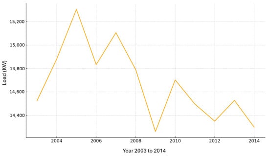
Figure 2.
Load data pattern before normalization.
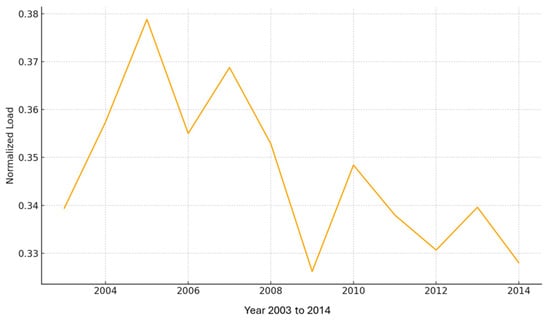
Figure 3.
Load data pattern after normalization.
Although this study focuses on STLF, capturing long-term dependencies from historical data is crucial. Electric load at a given time is influenced by patterns observed in previous days and weeks. Modeling these dependencies enables the LSTM-RNN to better capture recurring daily, weekly, and seasonal trends, enhancing short-term forecasting accuracy.
3.2. Data Investigation
An essential initial phase in the process is thorough data investigation to identify the fundamental connections and patterns in the dataset. This includes three sub-analytical steps: electrical load behavior analysis, sensitivity analysis, and correlation analysis. Through assessing a statistically significant relationship between the target variable (electrical load) and input features (such as time, temperature, or seasonality), correlation analysis sheds light on the significance of the features. Sensitivity analysis helps determine the variables with the greatest impact on forecast accuracy by examining the detailed effect of each input on the model’s output. To identify consumption peaks, recurring variations, and deviations in electrical load behavior, this research additionally evaluates daily, monthly, and seasonal load variation patterns.
3.2.1. Correlation Analysis
A correlation matrix is an analytical technique that shows how strongly many variables in a dataset have a linear relationship with one another. The numbers in the matrix indicate the Pearson correlation coefficient between two variables. A perfect positive correlation is represented by a value of +1, and a perfect negative correlation by a value of −1. A value of 0 implies no linear link. So, the Pearson correlation coefficient can be represented as follows [26,27]:
Equation (1), where ‘rxy’ represents the two variables ‘x’ and ‘y’. ‘xi’ and ‘yi’ are the individual sample points, ‘’ and ‘’ are the means of data variables, and ‘n’ is the total number of observations. In electrical load forecasting, the correlation matrix helps identify which input feature (temperature, hour, month, etc.) from the dataset is most closely related to the load values, thereby reducing dimensionality and enabling effective feature selection [28].
In Figure 4, the dataset’s correlation matrix is shown, normalized to reveal the linear correlations between input features and the targeted variable, Normalized_load. With a remarkable 0.50 correlation between the variable hour and Normalized_load, it is evident that the power demand varies significantly throughout the day, most probably as a result of variations in human behavior, like morning and evening peak usage. Since demand directly affects the load value, it also exhibits a significant correlation of 0.50 as predicted. With an average correlation of 0.21, the changeable temperature suggests that load is influenced by ambient temperature, possibly due to heating or cooling considerations. In contrast, there is little direct linear influence on short-term load change from characteristics such as year, month, day, and weekday, which show very weak correlations (range between −0.03 and 0.02). If these features are treated nonlinearly, they might still help capture category or seasonal patterns. It is highly recommended that the LSTM model incorporates hour, demand, and temperature, since they are the most significant factors for load forecasting.
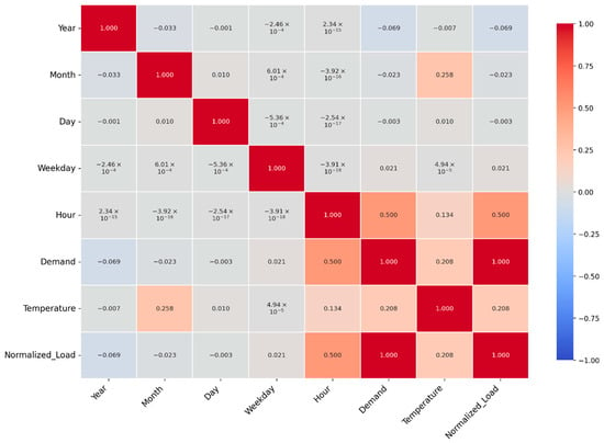
Figure 4.
Correlation coefficient matrix for all the single attributes in the normalized load dataset.
3.2.2. Sensitivity Analysis
Sensitivity analysis measures how variations in input variables affect a model’s output. It helps identify which factors, like demand, temperature, or hour, have the most significant impact on the anticipated load values throughout the electrical load forecasting process. Sensitivity analysis measures the relationship between a particular characteristic and the model’s output by methodically changing one input at a time while holding the rest constant. This assists with feature prioritization and improves model performance optimization, dependability, and interpretability. Furthermore, this procedure ensures the forecasting model is influenced by the most pertinent inputs, resulting in more reliable and accurate predictions.
Figure 5 shows the sensitivity analysis, which is carried out using permutation importance, and highlights the relative contribution of each input feature to the load forecasting model’s prediction ability. ‘Temperature’ is the most significant factor influencing load variation among all the variables with the highest mean relevance. A significant seasonal trend in electricity use is indicated by the second most sensitive parameter, ‘Month’, which may be related to changes in the climate or usage patterns throughout the year. The moderate-to-low importance of features like weekday, day, and year suggests that they are not among the primary factors, but these parameters add some contextual value. Hour has a relatively low sensitivity, which might indicate that its predictive power is already captured by other temporal variable changes that are controlled internally by model dynamics. As per this paper, temperature and month should be given priority when entering data into the model. To increase efficiency, less essential variables may be improved or eradicated during model optimization.
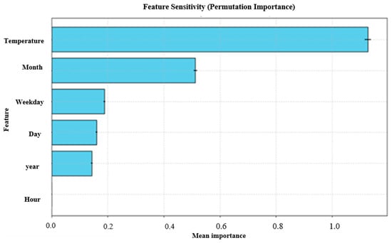
Figure 5.
Sensitivity analysis of the dataset.
3.2.3. Electrical Load Behavior Analysis
Identifying electrical load behavior patterns over time scales significantly contributes to increasing the precision and dependability of load forecasting. Subsequently, it can be performed to identify long-term sequences like annual demand, seasonal variations, or distribution of load demand in terms of hour changes by analyzing electric load demand data from 2003 to 2014. Figure 6, Figure 7 and Figure 8 show the distribution of the electric load using graphs.
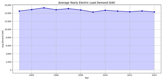
Figure 6.
Distribution of average yearly electric loads in (kW) from 2003 to 2014.
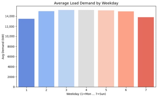
Figure 7.
Distribution of the average electric load demand by weekday from 2003 to 2014.
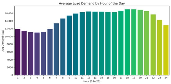
Figure 8.
Distribution of the average electric load demand by hours of the day.
According to the plot in Figure 6, the average demand fluctuated between 14,200 kilowatts (kW) and 15,300 kW over the 12 years. Each point represents the average annual load in kW for the corresponding years. In 2006, we saw the highest demand, which was followed by a modest decrease in 2007 and another modest peak in 2008. In 2009, the load exhibited a slow, gradual decline with just slight annual fluctuations. In 2010 and 2014, we saw the demand fall to its lowest level, suggesting potential shifts in consumer behavior, system effectiveness, or economic conditions during those years.
Figure 7 demonstrates how the demand for electrical load is distributed throughout the week. Weekday values are shown as numbers (1 = Monday to 7 = Sunday). The average load is indicated on the vertical axis in kW. Weekdays, particularly Tuesday through Friday, have the largest average demand, reaching values of almost 15,000 kW, according to the graph, while Monday 1 and Sunday 7 have the lowest average demand, which ranges from 13,500 to 13,800 kW. This pattern represents normal human activity and industrial behavior. Energy consumption tends to decrease on weekends and early in the week, probably because of fewer business activities or staggered starts, while it tends to grow during the workday due to increased commercial and industrial operations.
Figure 8 shows the hourly fluctuation in power demand over 24 h, expressed in kW, for the average load demand each hour of the day. Demand reaches its lowest point between 1 and 5 AM, when it drops to about 2000 kW. This happens because most people are asleep at that time. After five in the morning, when morning routines and business operations take place, there is a gradual increase in demand that lasts until three in the afternoon, when it reaches a plateau of 8000–10,000 kW. Early in the evening, between 5 and 6 pm, the most prominent peaks occur, reaching 14,000 to 15,000 kW, which reflects an increase in residential and commercial activity as people head back home. Demand gradually declines throughout the night. With peak times demanding more grid capacity and off-peak hours potentially providing possibilities for cost savings, this chart illustrates typical cycles of energy usage.
3.2.4. Time-Series Analysis for Electrical Load Demand
To determine the electrical load on a daily, weekly, and monthly basis, time-series analysis is necessary. Figure 9 and Figure 10 show demand over time. It is possible to determine whether the data is random, recurring, or seasonal with the use of this procedure. Additionally, this approach only shows a few statistical measures to illustrate the distribution of specific dataset figures.
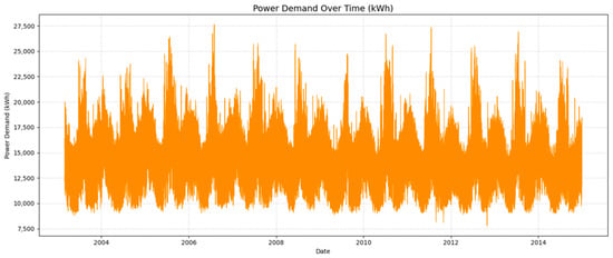
Figure 9.
Power demand in (kWh) from March 2003 to December 2014.
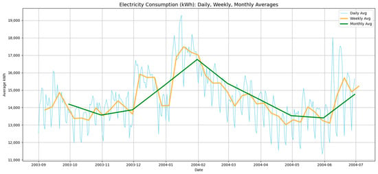
Figure 10.
Electricity demand over the time period (September 2003 to December 2004).
From March 2013 to December 2014, the graph in Figure 9 shows the amount of power consumed (kWh), showing steady overall usage and seasonal peaks (probably due to summer and winter requirements). Although the x-axis labels (2004–2014) are out of sync with the data, power demand varies between 7500 and 27,500 kWh. With its consistent seasonal fluctuations and lack of long-term growth or reduction, it is helpful for energy planning.
Figure 10 shows the (daily, weekly, and monthly) average usage of power in kWh, illustrating the patterns of consumption from September 2003 to July 2004. With the transition from summer demands to winter temperatures, the monthly averages show a slow decline in use from September 2003 to January 2004. The minimal electricity usage from February to April 2004 coincided with constant energy needs. This information reveals that the power demand fluctuates seasonally, peaking during months of severe weather and decreasing during times of moderate temperatures.
3.3. Forecasting Methodology
This section discusses the proposed method for predicting long-term forecasting using DL algorithms on a real dataset, as shown in Figure 11. After feature selection and dataset normalization are complete, the procedure begins. Following that, LSTM-RNN, BPNN, KNN, and ANN DL models are used for model training to make long-term predictions based on historical data. Then, the ML models’ hyper-tuning parameters, such as learning rate, epochs, batch size, hidden layers, optimizer, etc., are adjusted, and performance metrics are used to evaluate each model’s correctness. Finally, we select the optimal load forecasting method. Pandas 2.2.3, Seaborn 0.13.2, Matplotlib 3.10.0, TensorFlow 2.15, NumPy 2.0.2, Google Colab, Python 3.10, and Sklearn 1.6.0 were used to implement all of these models for this forecasting.
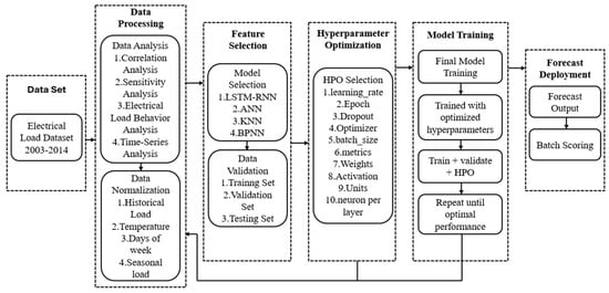
Figure 11.
Methodology of electrical load forecasting using machine learning (ML) algorithms.
3.3.1. Data Processing
- Data normalization for load forecasting
Data normalization is a preprocessing process that is essential to improving model accuracy and performance in electrical load forecasting since it prevents some features from overpowering all other features. There are several kinds of normalization techniques, such as Z-score, min–max, and standardization. For this research, the min–max normalization method has been used. To help DL models like LSTM converge more quickly and prevent bias toward characteristics with higher numeric ranges, it converts input features like load, temperature, or time into a standard scale (between 0 and 1). The min–max data normalization process is given below [29]:
where ‘X’ is the original value, and ‘X min’ and ‘X max’ are the minimum and maximum values from the dataset, respectively.
Highly valued variables, such as (load in kilowatts), could dominate minor features (hour or temperature) when the values of the datasets are in abnormal positions, resulting in unstable training or ineffective accuracy. Hence, normalization is a crucial preprocessing step in load forecasting to guarantee uniform scaling, quicker training, and more accurate predictions.
- 2.
- Feature selection for load forecasting
The most significant step in load forecasting is the feature selection, which aims to determine the most pertinent input variables impacting power demand. Identifying the correct features for forecasting models, particularly those features that use ML and DL, can increase model accuracy, decrease overfitting, and speed up training [30]. In electrical load forecasting, typical features include temperature, time of day, day of the week, season, historical load, and often humidity, holiday indicators, or economic activity levels. These variables are chosen using statistical techniques such as correlation analysis, mutual information, and permutation importance, along with domain expertise [31]. In this work, sequence creation through lag-based features has been applied, where the model learns patterns from the previous time steps of the target variable [32]. The lag order means the number of past observations used as input is determined based on autocorrelation behavior and domain knowledge of electric load patterns. Because electricity demand shows strong hourly and daily dependencies, selecting a 24 h lag window allows the model to capture short-term temporal variations effectively and contributes to higher forecasting accuracy.
- 3.
- Selecting an LSTM-RNN model for forecasting
An LSTM-RNN model for STLF is highly justified by the dataset’s features. The hourly load data from 2003 to 2014 shows various time-dependent patterns, including daily, weekly, and seasonal cycles, as well as long-range correlations that are partially influenced by temperature fluctuations. Because traditional models like ANN, BPNN, or KNN lack mechanisms for storing long-term sequential information, these models have an obstacle to capturing such recurrent and nonlinear patterns. LSTM networks, on the other hand, are ideally suited for learning temporal dependencies and temperature load interactions as they employ gated memory units that enable the model to store, update, and forget information effectively. Moreover, traditional RNNs’ vanishing-gradient issue is solved by LSTMs, allowing for stable learning over multiyear hourly sequences. Hence, the LSTM-RNN model is the best option for precise short-term load predictions based on both the observed dataset characteristics and the intrinsic capabilities of the architecture.
3.3.2. Machine Learning Algorithms
The following section provides an overview of the four ML algorithms that were used. The accuracy and performance of these algorithms were taken into consideration when selecting them. However, these ML algorithms, which may have similar objectives, are distinguished by their mathematical models, advantages, and disadvantages. Evaluation of the dependent values that could be predicted by the independent variables that differ between elements is performed using a DL technique. In this paper, four types of neural networks, LSTM-RNN, BPNN, KNN, and ANN, were used to forecast electrical load.
- LSTM Using a RNN
Electrical load forecasting is an instance of a forecasting application that effectively predicts time-dependent variables using a hybrid model combining recurrent neural networks and LSTM units. LSTMs overcome the limitations of traditional RNNs, particularly the vanishing-gradient problem, through memory cells regulated by input, output, and forget gates [33]. The design may be able to capture both transient variations and long-term seasonal trends in load profiles. Our research proposed an LSTM-RNN-based hybrid model using historical hourly load data. The model architecture consists of a dense output layer, one 64-unit LSTM layer selected to balance model complexity and computational efficiency by providing sufficient capacity to capture nonlinear load dynamics without overfitting, and one input layer. The data was normalized and framed into sequences using a 24 h look-back frame to forecast the load for the following hour. MSE was used as a loss function, and the Adam optimizer was used to train the model. The LSTM-RNN technique successfully learns from past trends and generates accurate predictions, according to evaluation using metrics like MAE, RMSE, MAPE, and R2:
In Equation (3), the compressed formulation of the LSTM-RNN forecasting model is represented mathematically, where the hidden state ‘’ and cell state ‘’ at time t are calculated by transforming the current input ‘’ and previous states ‘’ using an LSTM. Temporal information is regulated by the model through the input gate ‘’, forget gate ‘’, output gate ‘’, and candidate cell ‘’. To accurately assess nonlinear and time-dependent load dynamics, these gates function together to control memory flow, ensure long-term dependencies, and reduce vanishing-gradient limitations [33].
RNN and LSTM forecasting are combined in a hybrid architecture shown in Figure 12. The model’s input layer analyzes sequential data before being sent to the first hidden layer, which is made up of RNN cells, which are good at identifying short-term dependencies. To capture long-term temporal trends and address problems like vanishing gradients, the output from this RNN layer is then fed into a second hidden layer made up of LSTM units. A fully connected layer further processes the LSTM layer’s outputs to extract pertinent features and patterns before sending them to the final output layer. This architecture is especially appropriate for forecasting tasks where both short-term variations and long-term patterns are crucial, such as electrical load prediction.
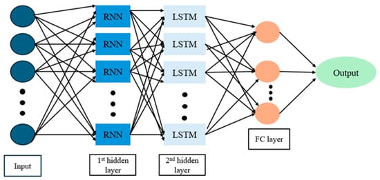
Figure 12.
A hybrid model of LSTM-RNN structure.
- 2.
- Backpropagation Neural Network
The block diagram in Figure 13 illustrates the three main layers that comprise a BPNN architecture: an input layer, one or more hidden layers, and an output layer. Parameters such as temperature, time, or past electrical demand ‘x1 to xm’ are the network inputs, which are sent to the input layer and then transmitted to the hidden neurons via the changes in weighted connections ‘Wij’ [34]. Each hidden neuron represents convoluted nonlinear interactions by calculating a weighted sum of inputs and applying a nonlinear activation function (such as a rectified linear unit) represented as φ with accompanying biases θ. After that, the output layer receives the activated outputs (a1 to aL) and generates the final prediction output ‘ok’, which, for regression tasks, is usually used for linear activation [34]. For the purpose of modifying weights and reducing loss, the backpropagation technique is used to propagate the error backwards:
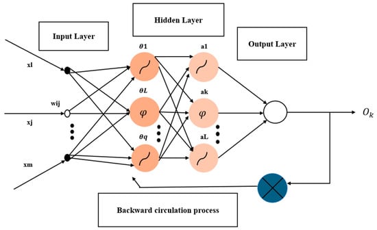
Figure 13.
The block diagram of BPNN.
In Equation (4), ‘y’ is the actual load and ‘’ is the predicted load, representing the squared error, and to reduce the prediction error from the network, BPNN produce a gradient-layer as shown below in Equation (5), where ‘’ is the current weight, ‘’ is the updated weight, ‘ƞ’ is the learning rate, and ‘’ is the gradient of the loss:
Through the network, after the prediction was performed, the error is determined by comparing the predicted value with the actual value. To increase forecast accuracy, this procedure iteratively continues during training. Moreover, BPNNs perform effectively for nonlinear load forecasting situations, while they may not be equally effective at addressing sequential dependencies as recurrent models like LSTM.
- 3.
- Artificial Neural Network
In Figure 14, the block diagram of an ANN is presented, which is a computational model that uses the structure and functions of the human brain as inspiration to find complex patterns and relationships in data. ANN consists of layers of interconnected nodes (neurons) called input, hidden, and output layers. Neurons use activation functions to add nonlinearity, and each connection carries a weight:
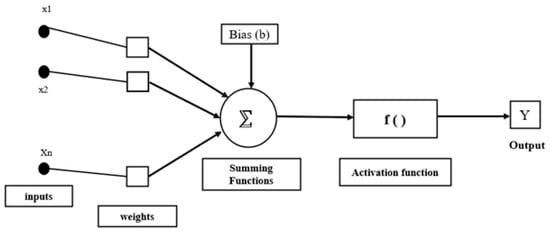
Figure 14.
The block diagram of an ANN.
ANNs are formed using interconnected neurons that use nonlinear activation and weighted summation to transform inputs into outputs, as shown in Equation (6), where ‘’ is the input variables, ‘’ is the weight connecting input i to neuron j, ‘’ is the bias, ‘f’ is the activation function, and ‘’ is the output of neuron j. Hence, ANNs are suitable for nonlinear regression issues in the framework of electrical load forecasting since they can represent complex interactions between input features like time and historical load levels. However, compared to the hybrid model, recurrent LSTM-ANN are less effective at predicting time series due to their inability to capture temporal dependencies.
- 4.
- K-Nearest Neighbors:
KNN is an instance-based learning algorithm widely used for both classification and regression problems. Utilizing a distance measure like Euclidean distance, KNN finds the ‘K’ most comparable occurrences (neighbors) in the historical dataset to predict the output for a given input in a situation of electrical load forecasting [35]. Equation (7) represents the Euclidean distance for KNN, where ‘x’ is the test input, ‘’ is the ith training input, and ‘n’ is the total feature. Based on this, KNNs select the smallest metrics:
Frequently, the average of the outputs from the neighbors yields the predicted value. The red dot point in Figure 15 indicates the location where a load prediction is produced. It finds the nearest neighbors, and the outcome is inferred from their values. Although KNN’s interpretability and simplicity make it useful, it can become computationally costly when dealing with huge datasets and is unable to simulate intricate temporal patterns [36].
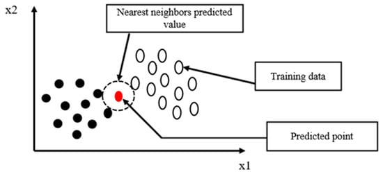
Figure 15.
The block diagram of KNN.
After the overall discussion of individual methods, a comparative analysis of the advantages and disadvantages of DL methods is given below in Table 4.

Table 4.
Advantages and disadvantages of deep learning (DL) methods.
3.4. Temperature Analysis for Forecasting
In the LSTM-RNN model, temperature is an independent input feature, as initial analysis showed a significant relationship between ambient temperature and load consumption. Before training, temperature was normalized using the same scaling technique as the load demand and included in the feature matrix when creating the LSTM sequences. This enables the network to receive temperature data at each time step along with historical load data. The LSTM is able to capture nonlinear effects, such as increased load during high heat or decreased demand during milder temperatures, by learning to store, update, or discard temperature-related data through its gated memory units. Its significance has been proved by analyses with and without the temperature feature, which enhanced the MAE, RMSE, and MAPE results. These findings show that temperature plays a crucial role in STLF, significantly improving the model’s accuracy in forecasting.
The dataset’s annual, monthly, and weekly temperature fluctuations are illustrated in Figure 16. In the curve, monthly averages record steadily rising temperatures during the middle of the year, followed by an average fall, and seasonal analysis reveals clear differences between winter, spring, summer, and autumn. Weekly averages show short-term variations while remaining largely consistent. These patterns reflect the dataset’s finding of a significant correlation between fluctuation in temperature and power consumption.
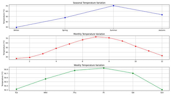
Figure 16.
Seasonal, monthly, and weekly time variance curves.
3.5. Hyper-Parameter Tuning for Deep-Learning Models
The hyperparameters used in this research to achieve the best output for the investigated models are displayed in Table 5 of this section. This section explores the optimal tuning parameters with a search space that determines the structure of models to estimate electrical loads, a technique known as hyperparameter tuning.

Table 5.
Deep-learning models’ hyperparameter-tuning methods.
3.6. The Selection of Metrics
Several kinds of metrics related to data regression statistically evaluate its performance [37]. Four widely employed statistical measures were used to evaluate the forecasting models’ accuracy and reliability: MAE, MAPE, RMSE, and R2. These measures were selected because they provide an in-depth assessment of the model’s overall fit quality and its percentage of prediction error, which makes them appropriate for regression tasks like electrical load forecasting:
- Mean Absolute Error (MAE): MAE determines the average size of a set of forecast mistakes without taking into consideration the direction of the errors’ advantage. There are fewer abnormalities, and it is easier to comprehend. Equation (8) describes the calculation of MAE, where is the actual data value, is the predicted data value, and n is the number of observations:
- 2.
- Mean Absolute Percentage Error (MAPE): Prediction accuracy can be expressed as a % by MAPE, which facilitates cross-scale dataset comparison. When the real values are near 0, it could be sensitive. The calculation of MAPE is described in Equation (9):
- 3.
- Root Mean Squared Error (RMSE): The square root of the average squared differences between expected and actual values is measured by RMSE. Compared to MAE, it penalizes greater errors more. Equation (10) shows the calculation process of RMSE:
- 4.
- Coefficient of Determination (R2): R2 indicates a metric’s capacity to explain variance in real values. When the value is close to 1, the predictive potential is significant [38]. Equation (11) is the calculation of the R2:
- 5.
- Mean Squared Error (MSE): Mean squared error (MSE) is a commonly employed statistic to assess regression models. It determines the meaning of the squared deviations between the actual and expected values. Since squaring the error rates ensures larger errors are penalized more severely, MSE is particularly sensitive to outliers. Equation (12) is the calculation process of MSE:
4. Results and Discussions
The ability of the DL models is evaluated using evaluation metrics on deployment. The predicted results of ML algorithms and performance metrics, which rely on determining each algorithm’s MAPE, MSE, R2, RMSE, and MAE (these algorithms are unitless, as they inherit the normalized target variable’s scale directly, while MAPE is expressed in percentage), are provided in this part.
4.1. Forecasting Results
A variety of ML models, including LSTM-RNN, KNN, BPNN, and ANN, were evaluated for their prediction accuracy and generalization potential by assessing forecasting performance with and without hyperparameter tweaking adaptation. Optimization algorithms, including Keras Tuner, GridSearchCV, and RandomizedSearchCV, were used to compare each model’s tweaked counterpart to its baseline configuration. Important performance metrics, including R2, MAE, MSE, MAPE, and RMSE, were the primary objectives of the analysis. The outcomes indicated that model performance was significantly impacted by hyperparameter modifications, which frequently increased forecasting accuracy. The following section presents the results obtained from different DL models with and without hyperparameter tuning.
4.1.1. Forecasting Using Different Machine Learning Models
This subsection presents a comparative analysis of forecasting accuracy obtained using different ML models, namely LSTM-RNN, BPNN, KNN, and ANN, as illustrated in Figure 17. For all parametric neural network models (LSTM-RNN, BPNN, and ANN), training is performed using the Adam optimizer. The KNN model is non-parametric and generates predictions based on distance-based similarity without an explicit training process.
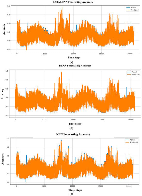
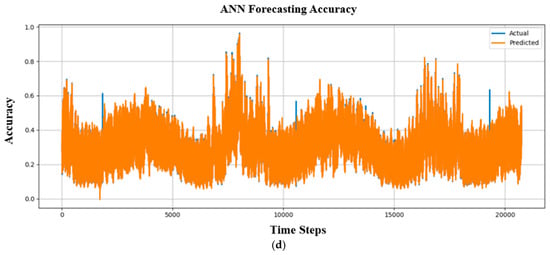
Figure 17.
Forecasting accuracy comparison between actual and predicted outputs without hyperparameter tuning for (a) LSTM-RNN, (b) BPNN, (c) KNN, and (d) ANN.
Figure 17 shows the temporal evolution of forecasting accuracy across approximately 20,000 time steps. In each subfigure, the blue curve represents the actual values, while the orange curve denotes the predicted values. A close overlap between the two curves indicates stable and consistent forecasting performance over time. As shown in Figure 17a, the LSTM-RNN model maintains a high level of alignment between actual and predicted accuracy trends over extended time horizons. Although minor deviations occur during periods of rapid variation, the overall temporal behavior is well preserved. This indicates that the LSTM-RNN effectively captures long-term temporal dependencies, which are important for maintaining stable accuracy in STLF tasks.
The BPNN results in Figure 17b demonstrate reasonable agreement between actual and predicted accuracy values. However, larger deviations are observed during dynamic periods. This suggests that while BPNN can model nonlinear relationships, it has limited capability in retaining temporal information compared with recurrent architectures. Figure 17c shows the forecasting accuracy of the KNN model. The predicted accuracy values exhibit noticeable inconsistencies with the actual values, particularly during high-variation intervals. This behavior reflects the limitations of distance-based, non-parametric methods in modeling complex time-dependent patterns in electric load data. The ANN results presented in Figure 17d indicate partial alignment between predicted and actual accuracy values. While ANN captures general trends, the absence of recurrent memory restricts its ability to maintain consistent accuracy under varying temporal conditions.
Quantitative performance metrics are summarized in Table 6. Although the ANN model achieves the lowest MAE and MAPE values, the proposed LSTM-RNN model demonstrates consistently low error levels across all evaluation metrics (MAE, MSE, RMSE, and R2), combined with stable accuracy behavior over time. These results indicate that the LSTM-RNN offers a balanced trade-off between numerical accuracy and temporal stability, making it well-suited for STLF applications. The proposed model is therefore not claimed to be universally superior, but rather to provide robust and reliable performance when compared with classical benchmark methods.

Table 6.
Results of each forecasting machine learning model.
4.1.2. Forecasting Using Hyperparameter Tuning Between Different MachineLearning Models
Figure 18 represents the electrical load forecasting using hyperparameter-tuned (learning rate, optimizer, dropout, epochs, metrics, etc.) to increase the model’s efficiency and overall performance further. Table 7 provides the hyperparameter-tuned result values of the models. The LSTM recurrent neural model tuning results in a MAPE of 1.60%, which is significantly more efficient than other models. Additionally, the MAE of 0.0048 indicates that the system’s overall accuracy surpasses that of other models.
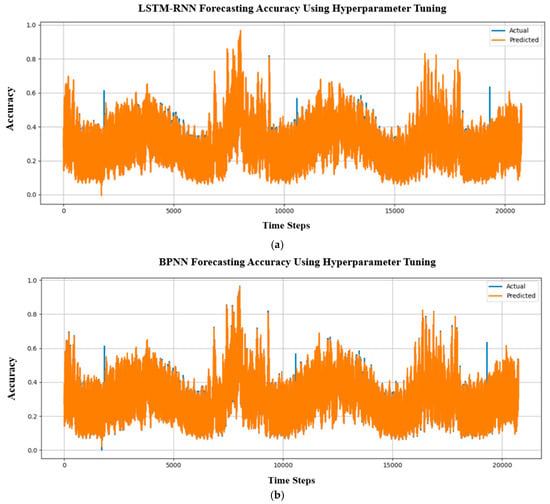
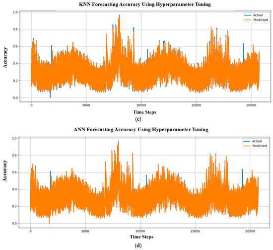
Figure 18.
Forecasting accuracy comparison between actual and predicted hyperparameter tuning outputs for (a) LSTM-RNN, (b) BPNN, (c) KNN, and (d) ANN.

Table 7.
Results of each forecast using hyperparameter-tuned ML models.
The predicting capability for electricity load values across time steps up to 20,000 is demonstrated by the hyperparameter tuning results for the four neural network models in Figure 18. Effective tuning for capturing time-dependent trends is provided by the LSTM-RNN model’s structured alignment between actual and predicted values. Although the data supplied is less precise, the BPNN results show a focus on time periods, indicating that periodic load trends may improve. Though time ranges and periods are mentioned in the KNN model’s output, limited data indicates that even after adjustment, the model would still have trouble with the complexity of time-series forecasting. Furthermore, although the ANN model’s performance is less interpretable due to the lack of specific accuracy measurements, it shows discrete time-step markers, which indicate systematic evaluation. The LSTM-RNN demonstrates that it is the most reliable overall, but more metrics or greater refinement may be needed to properly evaluate the other models’ tuned performance.
Due to their capacity to handle temporal dependencies through built-in memory cells that learn patterns across time steps, hyperparameter-tuned LSTM-RNNs perform better in electricity load forecasting than other neural networks (BPNN, ANN, and KNN), as illustrated in Figure 19. This is especially important for load forecasting, where load demand is dependent on historical patterns. To prevent overfitting and capture both short-term fluctuations and long-term trends, such as daily cycles and seasonal changes, LSTMs can optimize hyperparameters like layer depth, dropout rates, and hidden units. In comparison with simpler networks that have trouble with time-series data, their gated architecture (input, forget, and output gates) automatically maintains pertinent past information and eliminates noise. As demonstrated by the outcomes, which consistently retain higher performance (+0.10 accuracy increases to +0.11) throughout all time steps when compared to other models, LSTMs are able to attain superior accuracy by leveraging a combination of architectural advantages and targeted efficiency improvements.
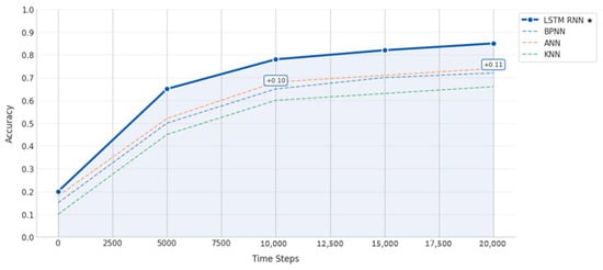
Figure 19.
Overall accuracy of neural networks.
Figure 20, the training vs. validation loss curve of the tuned LSTM–RNN model, shows a sharp decline in both losses over the first few epochs, followed by stable convergence with a slight gap between them. The model’s adaptation to temperature-driven variance in the data is reflected in the validation loss’s initial slight fluctuation, but after hyperparameter tuning, the losses closely align, indicating faster convergence, lower final MSE, less overfitting, and improved generalization to unseen temperature conditions.
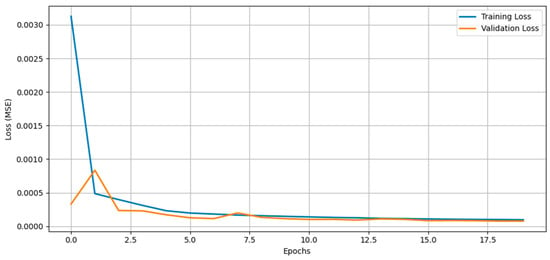
Figure 20.
Training vs. validation loss curve of LSTM-RNN after hyperparameter tuning.
The MAE and MAPE comparison graphs illustrate the impact of hyperparameter tuning across models in Figure 21 and Figure 22. The LSTM-RNN showed the most significant improvement, with its MAE reducing by 36.8% (from 0.0076 to 0.0048) and MAPE decreasing from 3.10% to 1.60%. While MAE decreased for all models, ANN continuously maintained low errors (MAE 0.0064 to 0.0059, and MAPE 1.85% to 1.72%), whereas KNN continued to be the least reliable, even after tuning (MAPE 4.91% to 3.74%). These results demonstrate the higher tuning adaptability of LSTM-RNN, but the stable performance of ANN points to a near-optimal initial setup.
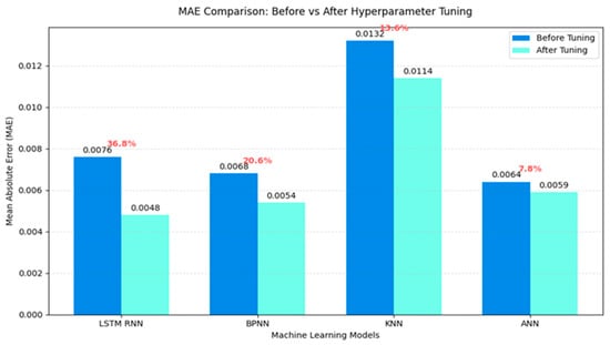
Figure 21.
MAE comparison graph between with and without hyperparameter tuning for forecasting.
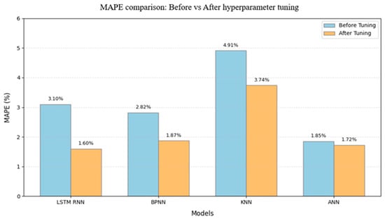
Figure 22.
MAPE comparison graph between with and without hyperparameter tuning for forecasting.
In contrast with previous models and findings from related research, the comparative results unequivocally show that the suggested hyperparameter-tuned LSTM-RNN achieves better predictive accuracy. In this study, the optimized LSTM-RNN reduced MAPE to 1.60% and MAE to 0.0048, outperforming ANN (1.72% MAPE, 0.0059 MAE) and BPNN (1.87% MAPE, 0.0054 MAE) using the same dataset and settings. However, KNN remains the least successful (3.74% MAPE, 0.0114 MAE). When comparing ML models on forecasts with published results, E.A. Madrid et al. (2021) [21] reported MAPE of 2.5–3.0%, while M. Zulfiqur et al. (2022) [16] used FE-BNN-BO optimization to reach roughly 2.1% MAPE. Error levels in irregular load scenarios were generally kept between 1.8 and 2.2% by even sophisticated RNN-based techniques by Wang et al. (2021) [19] and Q.C. et al. (2021) [20]. By assumption, if these models were tested on the same Bangladesh PDB dataset, their accuracy would likely remain above 2%, since they lack the combined effect of LSTM cells and systematic hyperparameter tuning. Hence, by reducing prediction error to almost half of traditional ML techniques and attaining a more stable convergence profile, the proposed strategy not only surpasses initial values but also exceeds a significant number of external comparisons. This efficiency is further evident in the RMSE of 0.0091, which indicates a smoother error distribution across time steps compared to ANN (0.0095) and BPNN (0.0094), and it is far better than KNN (0.0167).
5. Conclusions
The proposed research compared multiple neural networks, including ANNs, KNN, back propagation neural networks, and RNNs for long short-term electrical load forecasting to provide an in-depth analysis of hyperparameter-tuned DL models for long short-term forecasting. The findings show that the LSTM-RNN outperformed other models with the highest predicting accuracy, with a MAPE of 1.60% and an MAE of 0.0048, after being improved using methods such as Keras Tuner. Additionally, the ANN demonstrated excellent performance, sustaining low error rates, MAPE 1.72%, indicating that it is appropriate for steady load patterns. However, even after the modification, KNN maintained the lowest accuracy MAPE of 3.74%, demonstrating its errors when addressing convoluted timing connections. The model’s performance was significantly enhanced by hyperparameter tuning, especially for LSTM-RNN, which improved its MAPE by 48.4% and decreased its MAE by 36.8% when compared to its baseline. Given that LSTM-RNN is the most reliable option for identifying long-term dependencies in dynamic power demand data, our results highlight the significance of model selection and tweaking in load forecasting.
The incorporation of external features like real-time weather data, economic indicators, and patterns of renewable energy generation to improve forecasting robustness, as well as the development of hybrid models that combine LSTM with cognitive mechanisms or converter structures to enhance prediction accuracy during anomalous load fluctuations, are a few of the promising paths that are suggested to further this research.
Author Contributions
Conceptualization, N.N.K., S.A. and A.I.; methodology, A.S.N.H., N.N.K., S.M., S.A.H. and L.J.A.; software, N.N.K. and S.A.; validation, H.M., M.S.A. and L.J.A.; formal analysis, S.A., A.I., M.S.A. and S.M.; investigation, A.S.N.H., S.A. and S.A.H.; resources, S.A., H.M., A.I. and L.J.A.; data curation, N.N.K., S.A., A.S.N.H. and L.J.A.; writing—original draft preparation, S.A., N.N.K., A.I. and A.S.N.H.; writing—review and editing, S.A., A.I., H.M. and S.A.H.; visualization, M.S.A., S.M. and S.A.H.; supervision, S.A., A.I. and H.M. All authors have read and agreed to the published version of the manuscript.
Funding
This research work was supported from the grant: International Research Collaboration Top # 500, no Grant 3776/B/UN3.FTMM/PT.01.03/2024.
Data Availability Statement
The data used in this study is cited with appropriate reference within the manuscript.
Conflicts of Interest
The authors declare no conflicts of interest.
Abbreviations
The following abbreviations are used in this manuscript:
| RNN | Recurrent neural network |
| ANN | Artificial neural network |
| KNN | K-nearest neighbors |
| BPNN | Backpropagation neural network |
| LSTM | Long short-term memory |
| MAE | Mean absolute error |
| RMSE | Root mean squared error |
| R2 | Coefficient of determination |
| MAPE | Mean absolute percentage error |
| RES | Renewable energy sources |
| ML | Machine learning |
| DL | Deep learning |
| AI | Artificial intelligence |
| HPO | Hyperparameter optimization |
| STLF | Short-term load forecasting |
References
- Chen, J.; Liu, M.; Milano, F. Aggregated Model of Virtual Power Plants for Transient Frequency and Voltage Stability Analysis. IEEE Trans. Power Syst. 2021, 36, 4366–4375. [Google Scholar] [CrossRef]
- Muzaffar, S.; Afshari, A. Short-Term Load Forecasts Using LSTM Networks. Energy Procedia 2019, 158, 2922–2927. [Google Scholar] [CrossRef]
- Ali, S.; Riaz, S.; Safoora; Liu, X.; Wang, G. A Levenberg–Marquardt Based Neural Network for Short-Term Load Forecasting. Comput. Mater. Contin. 2023, 75, 1783–1800. [Google Scholar] [CrossRef]
- Mehta, S.; Basak, P. A comprehensive review on control techniques for stability improvement in microgrids. Int. Trans. Electr. Energy Syst. 2021, 31, e12822. [Google Scholar] [CrossRef]
- Hou, H.; Liu, C.; Wang, Q.; Wu, X.; Tang, J.; Shi, Y.; Xie, C. Review of load forecasting based on artificial intelligence methodologies, models, and challenges. Electr. Power Syst. Res. 2022, 210, 108067. [Google Scholar] [CrossRef]
- Kong, W.; Dong, Z.Y.; Jia, Y.; Hill, D.J.; Xu, Y.; Zhang, Y. Short-Term Residential Load Forecasting Based on LSTM Recurrent Neural Network. IEEE Trans. Smart Grid 2019, 10, 841–851. [Google Scholar] [CrossRef]
- Muhtadi, A.; Pandit, D.; Nguyen, N.; Mitra, J. Distributed Energy Resources Based Microgrid: Review of Architecture, Control, and Reliability. IEEE Trans. Ind. Appl. 2021, 57, 2223–2235. [Google Scholar] [CrossRef]
- Liu, H.; Xiong, X.; Yang, B.; Cheng, Z.; Shao, K.; Tolba, A. A Power Load Forecasting Method Based on Intelligent Data Analysis. Electronics 2023, 12, 3441. [Google Scholar] [CrossRef]
- Ahmad, S.; Hasan, S.M.N.; Hossain, M.S.; Uddin, R.; Ahmed, T.; Mustayen, A.G.M.B.; Hazari, M.R.; Hassan, M.; Parvez, M.S.; Saha, A. A Review of Hybrid Renewable and Sustainable Power Supply System: Unit Sizing, Optimization, Control, and Management. Energies 2024, 17, 6027. [Google Scholar] [CrossRef]
- Jacob, M.; Neves, C.; Greetham, D.V. Forecasting and Assessing Risk of Individual Electricity Peaks; Springer International Publishing: Cham, Switzerland, 2020. [Google Scholar] [CrossRef]
- Pourdaryaei, A.; Mohammadi, M.; Karimi, M.; Mokhlis, H.; Illias, H.A.; Kaboli, S.H.A.; Ahmad, S. Recent Development in Electricity Price Forecasting Based on Computational Intelligence Techniques in Deregulated Power Market. Energies 2021, 14, 6104, Correction in Energies 2024, 17, 2266. https://doi.org/10.3390/en17102266. [Google Scholar] [CrossRef]
- Hammad, M.A.; Jereb, B.; Rosi, B.; Dragan, D. Methods and Models for Electric Load Forecasting: A Comprehensive Review. Logist. Sustain. Transp. 2020, 11, 51–76. [Google Scholar] [CrossRef]
- Ahmad, N.; Ghadi, Y.; Adnan, M.; Ali, M. Load Forecasting Techniques for Power System: Research Challenges and Survey. IEEE Access 2022, 10, 71054–71090. [Google Scholar] [CrossRef]
- Hakyemez, T.C.; Adar, O. Testing the Efficacy of Hyperparameter Optimization Algorithms in Short-Term Load Forecasting. arXiv 2024, arXiv:2410.15047. [Google Scholar] [CrossRef]
- Vardhan, B.V.S.; Khedkar, M.; Srivastava, I.; Thakre, P.; Bokde, N.D. A Comparative Analysis of Hyperparameter Tuned Stochastic Short Term Load Forecasting for Power System Operator. Energies 2023, 16, 1243. [Google Scholar] [CrossRef]
- Zulfiqar, M.; Gamage, K.A.A.; Kamran, M.; Rasheed, M.B. Hyperparameter Optimization of Bayesian Neural Network Using Bayesian Optimization and Intelligent Feature Engineering for Load Forecasting. Sensors 2022, 22, 4446. [Google Scholar] [CrossRef]
- Inteha, A.; Nahid-Al-Masood; Hussain, F.; Khan, I.A. A Data Driven Approach for Day Ahead Short-Term Load Forecasting. IEEE Access 2022, 10, 84227–84243. [Google Scholar] [CrossRef]
- Al-Jamimi, H.A.; BinMakhashen, G.M.; Worku, M.Y.; Hassan, M.A. Advancements in Household Load Forecasting: Deep Learning Model with Hyperparameter Optimization. Electronics 2023, 12, 4909. [Google Scholar] [CrossRef]
- Wang, J.; Chen, X.; Zhang, F.; Chen, F.; Xin, Y. Building Load Forecasting Using Deep Neural Network with Efficient Feature Fusion. J. Mod. Power Syst. Clean Energy 2021, 9, 160–169. [Google Scholar] [CrossRef]
- Chen, Q.; Zhang, W.; Zhu, K.; Zhou, D.; Dai, H.; Wu, Q. A novel trilinear deep residual network with self-adaptive Dropout method for short-term load forecasting. Expert Syst. Appl. 2021, 182, 115272. [Google Scholar] [CrossRef]
- Madrid, E.A.; Antonio, N. Short-Term Electricity Load Forecasting with Machine Learning. Information 2021, 12, 50. [Google Scholar] [CrossRef]
- Taleb, I.; Guerard, G.; Fauberteau, F.; Nguyen, N. A Flexible Deep Learning Method for Energy Forecasting. Energies 2022, 15, 3926. [Google Scholar] [CrossRef]
- Feng, W.; Deng, B.; Chen, T.; Zhang, Z.; Fu, Y.; Zheng, Y.; Zhang, L.; Jing, Z. Probabilistic net load forecasting based on sparse variational Gaussian process regression. Front. Energy Res. 2024, 12, 1429241. [Google Scholar] [CrossRef]
- Hidayat, I.; Abido, M.A. Deep Learning and Traditional Models for Wind Speed Forecasting in Saudi Arabia. ELECTRON J. Ilm. Tek. Elektro 2025, 6, 95–103. [Google Scholar] [CrossRef]
- Available online: https://www.kaggle.com/datasets/ashfakyeafi/pbd-load-history (accessed on 20 January 2025).
- Luo, T.; Zhu, D.; Liu, J.; Yang, S.; He, J.; Fu, Y. Research on short-term power load forecasting based on deep reinforcement learning with multiple intelligences. EAI Endorsed Trans. Energy Web 2025, 12, 1. [Google Scholar] [CrossRef]
- Yu, J.; Benesty, J.; Huang, G.; Chen, J. Optimal single-channel noise reduction filtering matrices from the Pearson correlation coefficient perspective. In 2015 IEEE International Conference on Acoustics, Speech and Signal Processing (ICASSP); IEEE: New York, NY, USA, 2015; pp. 201–205. [Google Scholar] [CrossRef]
- Hong, T.; Pinson, P.; Fan, S. Global Energy Forecasting Competition 2012. Int. J. Forecast. 2014, 30, 357–363. [Google Scholar] [CrossRef]
- Zhang, G.; Patuwo, B.E.; Hu, M.Y. Forecasting with artificial neural networks: The State of the Art. Int. J. Forecast. 1998, 14, 35–62. [Google Scholar] [CrossRef]
- Acito, F. Neural Networks. In Predictive Analytics with KNIME; Springer Nature: Cham, Switzerland, 2023; pp. 229–254. [Google Scholar] [CrossRef]
- Plevris, V.; Solorzano, G.; Bakas, N.; Seghier, M.B. Investigation of performance metrics in regression analysis and machine learning-based prediction models. In 8th European Congress on Computational Methods in Applied Sciences and Engineering; CIMNE: Barcelona, Spain, 2022. [Google Scholar] [CrossRef]
- Altman, N.S. An Introduction to Kernel and Nearest-Neighbor Nonparametric Regression. Am. Stat. 1992, 46, 175–185. [Google Scholar] [CrossRef]
- Alhashemi, K.; Altınöz, Ö.T. Electricity load forecasting models based on LSTM and GRU with their bidirectional recurrent neural networks. Ömer Halisdemir Üniversitesi Mühendislik Bilim. Derg. 2025, 14, 1372–1384. [Google Scholar] [CrossRef]
- Rumelhart, D.E.; Hinton, G.E.; Williams, R.J. Learning representations by back-propagating errors. Nature 1986, 323, 533–536. [Google Scholar] [CrossRef]
- Li, F.; Jin, G. Research on power energy load forecasting method based on KNN. Int. J. Ambient Energy 2022, 43, 946–951. [Google Scholar] [CrossRef]
- Muhammad, Y.N.; Kartini, U.T.; Peni, H. Hybrid KNN-LSTM Modeling for Short-Term Feeder Peak Load Forecasting. Syntax. Lit. J. Ilm. Indones. 2025, 10, 3622–3631. [Google Scholar] [CrossRef]
- Pohare, P.; Kashikar, K.M.; Wankhade, G.B.; Rajguru, A.V.; Ingle, P.T. Performance Analysis and Optimization of Player Selection Using Machine Learning Algorithms. Int. J. Eng. Technol. Manag. Sci. 2025, 9, 334–341. [Google Scholar] [CrossRef]
- Manzoor, M.F. Energy Load Forecasting with Machine Learning: Models, Metrics, and Future Directions. Prem. J. Artif. Intell. 2025, 4, 100018. [Google Scholar] [CrossRef]
Disclaimer/Publisher’s Note: The statements, opinions and data contained in all publications are solely those of the individual author(s) and contributor(s) and not of MDPI and/or the editor(s). MDPI and/or the editor(s) disclaim responsibility for any injury to people or property resulting from any ideas, methods, instructions or products referred to in the content. |
© 2026 by the authors. Licensee MDPI, Basel, Switzerland. This article is an open access article distributed under the terms and conditions of the Creative Commons Attribution (CC BY) license.
