Abstract
The storage tank plays a key role in solar thermal installations, as thermal stratification allows high temperatures to be maintained in the upper region while keeping the return temperature to the collectors low. This study analyses the influence of thermal stratification on short- and long-term performance of solar domestic hot water systems using a multi-node storage tank model. An algorithm was developed to compute temperature profiles along the height of a storage tank operating under time-varying temperature and flow-rate conditions. Time courses of temperatures and heat fluxes in a solar domestic hot water system were determined. In addition, the seasonal variation in the optimal locations for supplying the tank with water from the solar collector was identified. Annual simulations were performed for the climate of Kraków (Poland) and the domestic hot water demand of a single-family household. The results show that the effect of the degree of stratification on solar fraction and solar efficiency is small. It was also demonstrated that the effect of thermal stratification within the tank on stabilizing the temperature of the produced water is more significant than the effect associated with increasing the tank volume.
1. Introduction
Solar energy is a natural, environmentally sound and economically viable source of domestic hot water (DHW) production. A storage tank is an essential component of systems based on this energy source. Water in such tanks undergoes thermal stratification, which occurs naturally in environmental, industrial, and household systems. Due to density differences, hot water accumulates in the upper part of the tank, while cooler water remains at the bottom. In solar heating systems, this behaviour enables high temperatures to be supplied for domestic use while maintaining low return temperatures to the collectors.
Complete mixing of the tank corresponds to the minimum ability to perform useful work, that is, the lowest exergy level. A higher degree of stratification increases the system exergy. Thermal stratification in domestic hot-water storage tanks is therefore beneficial, and system design should promote its formation and preservation.
Early computational models of thermal storage simplified tank behaviour by assuming complete mixing of its contents. Braun et al. [1] showed that increasing the degree of stratification, expressed as the number of nodes, from 1 to 40 increases the solar fraction by only about 2%. This result suggests that the level of stratification has little effect on heating system performance. Duffie and Beckman [2] proposed the multi-node model, in which the tank is divided into N ideally mixed nodes connected by mass flow. This formulation allows a gradual transition from a fully mixed configuration (N = 1) to an ideally stratified one (N → ∞). The multi-node model subsequently became the foundation for most research on thermal energy storage. An alternative one-dimensional representation is the plug-flow model [2,3]. Among the classical studies, Kleinbach et al. [4] compared one-dimensional formulations and showed that multi-node models better represent temperature profiles inside storage tanks. The authors concluded that beyond 10 nodes, accuracy improves only marginally while computational cost increases linearly. They also highlighted that node configuration directly affects the predicted outlet temperature profile, making the choice of N a key modelling parameter.
Han et al. [5] reviewed various types of storage tanks exhibiting thermal stratification. Liu et al. [6] developed empirical correlations for estimating the degree of stratification, accounting for parameters such as the Reynolds number and the tank height-to-diameter ratio. Rosen [7,8] performed a theoretical analysis of temperature distributions in a stratified tank. Riebel et al. [9] presented simulation results for water heating in a thermally stratified tank, comparing analytical and numerical solutions of the governing equations. They examined water heating under sinusoidally varying inlet conditions and compared the computed temperatures with experimental measurements. The simulations covered a one-month period. Araujo [10] reported simulation results indicating that increasing the degree of stratification from 1 to 4 increases the solar fraction by 5–28%.
In parallel with model development, experimental studies have explored the impact of inlet devices, coil configurations, and tank geometry. Andersen and Furbo [11,12] performed theoretical and experimental studies on stratification devices, demonstrating that properly designed inlets can substantially reduce mixing and preserve stratification. Wang et al. [13] analyzed the introduction of PCM in the form of spherical capsules into a storage tank.
Although multi-node models provide a good balance between accuracy and computational efficiency for long-term simulations, they rely on empirical assumptions for mixing and heat transfer between nodes. High-resolution CFD studies have been essential for understanding detailed flow and mixing mechanisms. They have also been essential for quantifying mechanisms of thermocline formation and degradation, as well as for validating simpler models [14,15,16,17,18,19,20,21,22].
In addition to experimental and CFD-based studies, the literature emphasizes the need for consistent stratification indicators. Lou et al. [23] reviewed a wide range of metrics, from thermocline thickness to exergy-based efficiency, and recommended using dimensionless numbers such as Richardson and Peclet numbers to assess stratification stability. Janus [24] reviewed solar heating and storage technologies, highlighting the central role of stratification in reducing system losses. Barrasso [25] summarized advances in thermal energy storage for solar applications, emphasizing stratification as a design criterion for both short- and long-term operation.
Most available CFD and experimental studies focus on short-term analyses, typically covering single charging or discharging cycles under controlled laboratory conditions. These investigations are crucial for understanding the fundamental mechanisms of stratification formation and degradation. However, they do not fully capture the seasonal dynamics of real solar heating systems. Accurate system design and performance evaluation require accounting for long-term variations in solar irradiance, ambient conditions, and load profiles, which can affect the stability and overall benefit of stratification over extended periods. Bai et al. [26] conducted simulations to assess the influence of stratification on seasonal solar system performance, demonstrating that higher stratification levels increase collector efficiency and reduce auxiliary heating demand.
While short-term CFD and laboratory studies have clarified the fundamental mechanisms governing stratification, systematic analyses of its long-term impact on solar system performance under realistic climatic conditions remain comparatively scarce. This issue is particularly relevant in regions with pronounced seasonal variations in solar availability, where the interaction between stratification, solar input, and heating demand determines the overall energy balance.
Objectives and Scope of the Study
The present study investigates how the degree of thermal stratification in a storage tank, together with other system parameters, influences water heating in solar installations. The analysis includes time courses of temperatures, transferred heat, and performance indicators. Introducing a set of differential equations describing stratification into the general solar water heating model allows the temporal evolution of temperature profiles in the tank to be tracked and the degree of stratification to be visually assessed. Both short- and long-term heating scenarios were analyzed. The short-term analysis covered several days of operation, focusing on outlet temperature behaviour under dynamically varying inlet conditions including variable flow rates, variable inlet water temperatures, and randomly varying values. The long-term simulations represented real climatic conditions for Kraków (Poland) and DHW production in a single-family household. The model employed the concept of utilizability to determine the useful heat delivered by the system.
An algorithm was developed to determine temperature profiles in a storage tank over arbitrary periods of the year. The algorithm combines the calculation of long-term temperature evolution in a perfectly mixed tank with a method for determining water temperatures at individual tank levels (nodes) under stratified conditions. For each time step, this approach requires solving a system of differential equations within an iterative loop. Based on the developed algorithm, temperature profiles in the storage tank were generated. The algorithm also enables analysis of time-dependent changes in the locations at which the tank is supplied with water.
2. A Multi-Node Stratification Model
The storage tank was modelled as a system composed of N ideally mixed sections (nodes). The nodes are numbered starting from the top of the tank. Because each node is assumed to be perfectly mixed, the outlet temperature of the stream leaving a given node is equal to the fluid temperature within that node.
In addition to the storage tank, the system consists of a heat-producing loop (collector loop) and a load loop. Each loop supplies water to a single node in the tank. Water from the producing loop enters the tank at temperature Tc0 with mass flow rate . The tank is supplied with cold water at temperature TL0 and a mass flow rate . Water leaves the tank in two streams: from the bottom, supplying the producing loop at temperature T[N], and from the top, supplying the consuming loop at temperature T[1]. The flow arrangement for a three-node tank (N = 3) is shown in Figure 1a.
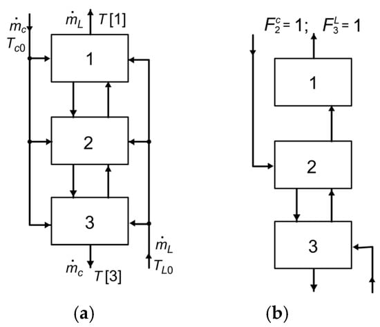
Figure 1.
Multi-node model. (a) General scheme; (b) Example of the flow arrangement corresponding to supplying the second node in the producing loop.
To maintain stratification in the tank, inlet streams are directed to nodes corresponding to their inlet temperatures. For example, when Tc0 < T[1] in the producing loop, the water is introduced into node 2. Similarly, the load loop is supplied according to the value of TL0; node 3, 2 or 1 is selected depending on the inlet temperature. Node 3 is supplied when TL0 < T[3].
For both loops, functions Fc and FL were defined to indicate the nodes to which the streams are delivered. A value Fc[i] = 0 means that the producing loop does not supply node i, whereas Fc[i] = 1 indicates that node i is supplied by this loop. Appendix B presents the algorithm used to determine the values of both functions. The energy balance for each node i = 1, 2, …, N is given by:
The heat accumulated in node i is expressed by:
The heat flow rate supplied from the producing loop to node i is given by:
The heat flow rate delivered to node i from the load loop (cold-water supply) is:
The mass flow rates between nodes i and i + 1 are defined as:
where
Based on the mass flow rates, the inter-node heat flows are determined as:
The heat flow rate exchanged with the surroundings is given by:
Consequently, the energy balance for node i takes the form:
The resulting model is described by a system of N ordinary differential equations. The initial conditions are specified as:
An example of the corresponding flow arrangement is shown in Figure 1b. It is assumed that the inlet temperature Tc0 is lower than T[1] but higher than T[2]; therefore the producing loop supplies node 2. At the same time, the cold-water stream (load loop) supplies node 3. For the flow arrangement shown in Figure 1b, the functions take the values Fc[2] = 1 and FL[3]= 1, while all other entries of Fc and FL are zero. The mass flow rate between nodes 1 and 2 is [1] = −, while that between nodes 2 and 3 is [2] = − .
To solve Equation (8), standard numerical methods for systems of ordinary differential equations are sufficient, such as the fourth-order Runge–Kutta method.
3. Simulation of Flow Through the Tank Under Variable Inlet Conditions
The analyzed tank is supplied with hot water from the top and with cold water from the bottom. The tank configuration is shown in Figure 2. For given inlet conditions, the value of T[1] depends on the degree of mixing in the tank, represented by the number of nodes N.
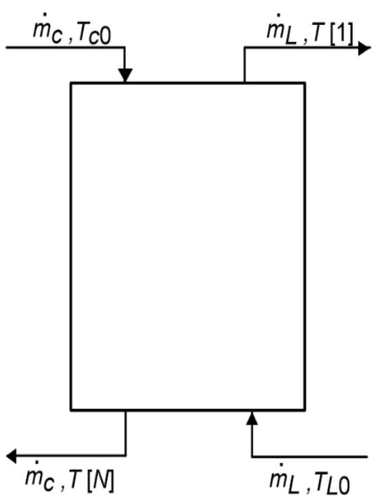
Figure 2.
Configuration of the tank considered in the analysis.
Figure 3 shows the time course of the outlet temperature for a tank supplied with a hot-water stream at a flow rate of 1.8 kg/min and an inlet temperature varying over a daily cycle according to:
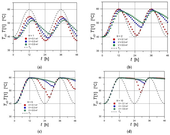
Figure 3.
The effect of tank volume V on the time courses of T[1] for fixed values of N. (a) N = 1; (b) N = 2; (c) N = 5; (d) N = 10.
The cold-water stream is supplied from the bottom at a flow rate of 0.2 kg/min and a temperature of TL0 = 10 °C. The temperature T[1] was calculated using the multi-node stratification model for various combinations of tank volume V and values of N representing the degree of stratification.
The dashed line indicates the time course of the hot-water inlet temperature Tc0. Figure 3a–d illustrate the influence of tank volume V at a fixed value of N. For ideal mixing (Figure 3a), a distinct drop in outlet temperature is observed, resulting from the immediate influence of the cold water supplied from the bottom. Stratification weakens this effect, which is already visible for N = 2 (Figure 3b), and becomes more pronounced for higher values of N. The smallest influence of the cold-water inflow occurs for large tank volumes and strong stratification (Figure 3d). In this case, the temperature T[1]—except for the initial transient during the first 12 h—remains close to 60 °C, corresponding to the maximum inlet temperature of the hot-water stream. Even for a small volume of V = 0.1 m3 and N = 10, the outlet temperature of the first node remains close to 60 °C for half of the daily cycle. A high degree of stratification therefore enables the outlet temperature to remain stable.
Stratification therefore has a clear stabilizing effect. To account for more realistic operating conditions, an additional random term was introduced to represent fluctuations in the inlet temperature. The variable Tc0′ was calculated according to:
where σ denotes the standard deviation. The random variable was assumed to follow a normal distribution. The deviations were generated using a random error generator (RND). Random numbers with a normal distribution were generated according to formula [27]:
where Ri denotes values of the random variable R with a uniform distribution in the interval (0,1). The generated values of X have zero mean and unit standard deviation.
Example time courses of Tc0′ for different values of σ are shown in Figure 4. For σ = 0, the profile follows directly from relation (10) and corresponds to the time courses shown in Figure 3. As σ increases, the spread of temperature values increases. In the subsequent analysis, σ = 3 was used. Figure 5 presents the time courses of T[1] for a tank supplied with water at temperature Tc0′. The comparison of the temperature profiles for N = 1 and N = 5 clearly shows that stratification reduces outlet temperature fluctuations.
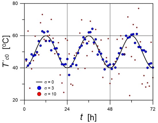
Figure 4.
Numerical generation of the temperature time courses Tc0′.
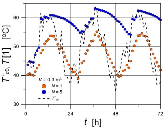
Figure 5.
Simulation of the time course of T[1] for a tank supplied with water of randomly varying temperature.
A simulation was also performed for the case in which the inlet cold-water flow rate, (equal to the outlet flow rate from the first node), varies according to:
The profile of this function corresponds to a situation in which the cold-water inflow is switched off during periods of low hot-water supply temperature. In Figure 6, the resulting temperature courses are presented. A strong influence of the number of nodes on the evolution of T[1] is evident. The differences between the profiles for N = 1 and N = 2 are particularly pronounced. During periods when Tc0 is close to its maximum value (60 °C), the outlet temperature T[1] reaches its minimum for the fully mixed tank (N = 1), in contrast to profiles obtained for higher values of N. For N ≥ 2, the values of T[1] do not fall below 50 °C. This means that for N = 1 (complete mixing throughout the tank volume), both the average level and stability of T[1] are reduced. In the considered case, the temperatures Tc0 and T[N] are not coupled; so the time course of Tc0 does not depend on the evolution of T[N]. Higher values of T[1] for N ≥ 2 therefore lead to a corresponding change in T[N], as dictated by the tank’s energy balance, but the variation in T[N] has no effect on the time course of Tc0.
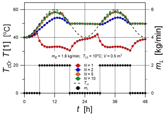
Figure 6.
Simulation of the time course of T[1] for a tank supplied with water at a time-dependent flow rate.
4. Solar Heating of DHW
4.1. System Description
The installation consists of solar collectors, a storage tank, an auxiliary heater, heat exchanger, and a mixing unit. The flow configuration of the system is shown in Figure 7. Devices responsible for fluid transport and measurement instrumentation are not included in the diagram.
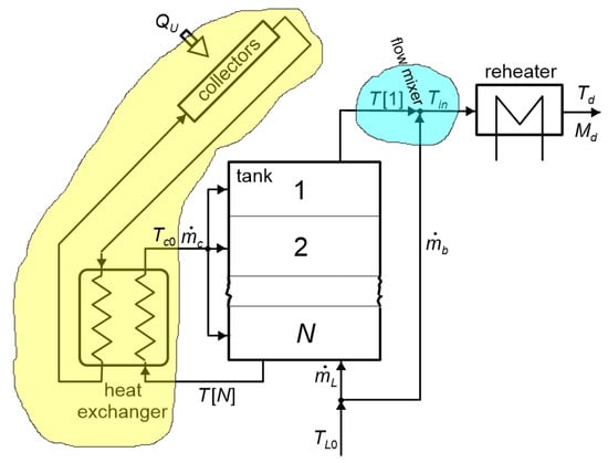
Figure 7.
Schematic of the DHW heating system.
The hot-water storage tank is modelled as a system composed of N ideally mixed nodes. Water from the producing (collector) loop enters the tank at temperature Tc0, while cold water (e.g., from the mains) at temperature TL0 is supplied from the bottom. Two streams leave the tank: water exiting from the bottom and feeding the collector at temperature T[N], and water exiting from the top at temperature T[1]. The flow rates through the tank are in the producing loop and in the consuming loop.
To supply domestic hot water at the required temperature, the system uses solar heat stored in the tank and/or heat delivered by an auxiliary heater. If the water leaving the first node has a temperature higher than the desired domestic hot-water temperature Td, it is mixed with a cold-water stream in the mixing unit before entering the domestic hot-water network. If the water temperature in the tank is below Td, the auxiliary heater is activated to raise it to Td. In this case, the cold-water bypass is switched off, and Tin = T[1].
4.2. Process Model
The calculations are based on the daily insolation on the collector surface, HT, for each day of the year. This value was determined from the insolation on a horizontal surface, H, and the coefficient R, defined as the ratio of total radiation on a tilted plane to that on a horizontal plane.
The coefficient R depends on the collector tilt angle, the clearness index, the fraction of diffuse radiation in the total radiation Hd/H, and the ground reflectance ρg, which depends on the local terrain. The values of H were taken from the literature [28] and approximated using the relation given in [29]:
The coefficient R was determined using the following relation [2]:
where Rb is the ratio of daily average beam radiation on the tilted surface to that on a horizontal surface. The time dependence of R was determined for a collector tilt angle of β = 60° and a diffuse reflectance ρg = 0.4. The resulting day-by-day values were approximated using the relation given in [30]:
The daily irradiation on the tilted plane, HT, is obtained as the product of H and R:
In the present model, the concept of solar utilizability, ϕ, is used. The daily utilizability ϕ is defined as the ratio of the useful energy gained during a day to the total solar energy incident on the collector over the same period. The quantity ϕ accounts for the fact that part of the incoming solar energy is not utilized during periods when the radiative flux is lower than the heat-loss rate from the collector to the surroundings. The critical solar irradiance, ITc, therefore plays a key role; it represents the irradiance level below which the collectors do not deliver heat to the system. The value of ϕ therefore depends on ITc and, indirectly, on the collector inlet temperature T[N], that is, the temperature in the Nth node of the tank. The relationships between these quantities are described using empirical expressions. These relations, as well as the procedure for determining utilizability ϕ according to Klein’s algorithm, are described in detail in the monographs by Duffie and Beckman [2] and by Chiasson [31].
4.3. Calculation Algorithm
4.3.1. Calculations for a Single Time Step
First, the daily irradiation on the collector surface, HT, was determined using relation (17). Based on the temperature in the last node, T[N], the critical solar irradiance ITc was calculated, followed by the utilizability ϕ. Using HT and ϕ, the useful heat produced by the collector during the day and delivered to the storage tank, Qu, was then obtained:
where Ac is the collector area and is the modified collector heat-removal factor. From Equation (A2), the expression for the collector outlet water temperature follows:
As a result of the mixing process described in Section 4.1, the inlet temperature to the auxiliary heater is the lower of Td and T[1], and thus:
If T[1] ≥ Td, then Tin = Td. If T[1] ≤ Td, then Tin = T[1]; and in this case the bypass flow is switched off ( = 0). In all cases, the inlet cold-water flow rate supplied to the tank, , can be determined from:
as given by Equation (A1).
Thus, for both streams supplied to the tank, the inlet temperatures Tc0 and TL0, as well as the flow rates and , are known. The system of differential Equation (8) can therefore be solved, allowing the temperatures in all tank nodes to be determined at the end of the time interval.
4.3.2. Calculations for Successive Days of the Year
Initial trial values of the water temperature in each tank node were assumed at the beginning of the year. For each day, the calculations consisted of determining the final temperatures in all nodes, which then served as the initial conditions for the following day. The computed final temperatures in the individual nodes on the last day of the year were required to match the assumed initial temperatures. As the convergence criterion, agreement of the temperature in the last node of the tank (i = N) within 0.1 °C was required. If this condition was not met, the calculations were repeated with a corrected initial condition.
For each day, the daily values of Qa and Qd were calculated. The daily amount of energy supplied by the auxiliary source is:
The daily amount of energy required to heat the desired mass of domestic hot water, Md, is:
The values of Qa and Qd were summed over all days of the year to obtain the annual quantities ΣQa and ΣQd. The difference between these values represents the annual amount of solar heat used for DHW production: ΣQs = ΣQd − ΣQa. Annual summation was also performed for the irradiation HT, yielding ΣHT. These totals provide the basis for determining the solar heating performance indicators SF and SE.
4.3.3. Calculation of Process Performance Indicators
The primary indicators are the solar fraction SF and the solar efficiency SE. The annual solar fraction is defined as the ratio of the solar energy used for water heating, ΣQs, to the total energy required for water heating, ΣQd:
where the summation is performed over all days of the year. For complete coverage of the heating demand by solar energy, SF = 1. The annual solar efficiency SE is defined as the ratio of the solar energy delivered for water heating, ΣQs, to the total solar energy incident on the collectors.:
If the solar energy incident on the collectors is fully used for water heating, then SE = 1.
5. DHW Heating—Calculation Results
The calculations were performed for different values of the operating parameters of the water heating installation, as indicated in the figure legends. The remaining numerical values, kept constant throughout the simulations, are listed in Table 1.

Table 1.
Data used in the simulations.
The modified collector heat removal factor applies to the case in which a heat exchanger is located between the collector and the storage tank (as shown in Figure 7). Consequently, there exists a circuit ‘c’ between the collector and the heat exchanger, and a circuit ‘t’ between the heat exchanger and the storage tank. The collector itself is characterized by the heat removal factor . The relationship between the factors and is given as follows [2,3]:
where the subscript min refers to either circuit c or t, depending on which mass flow rate product has the smaller value. In the calculations, = 1 and ε = 0.6 were assumed. The resulting value = 0.88 was used in the subsequent calculations.
In Figure 8, the time courses of H, R, and HT are presented, determined from relations (14), (16) and (17), respectively.
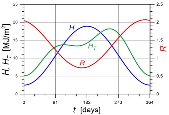
Figure 8.
The time courses of H, R and HT.
The temperature of the mains water varies throughout the year. Under the climatic conditions considered in this study, it ranges from 8 to 14 °C. Assuming that the minimum temperature occurs on day 14 of the year, its annual variation can be approximated by:
The temperature profiles at various places within the solar installation are shown in Figure 9. Throughout the entire period, the inequality T[1] > T[N] holds, although the temperatures in the extreme nodes differ only slightly. The inlet temperature to the auxiliary heater does not reach Td for approximately 125 days; during this period, the water must be heated by a non-solar source. The lowest curve represents the cold-water supply temperature TL0, given by relation (27). The figure also shows the time course of the mass flow rate of water entering the tank from the bottom. When T[1] < Td, the flow rate satisfies = Md/Δt, so the entire volume of cold water supplied to the system passes through the tank. For higher tank temperatures, part of the cold water bypasses the tank, resulting in the time-dependent behaviour of shown in the figure.
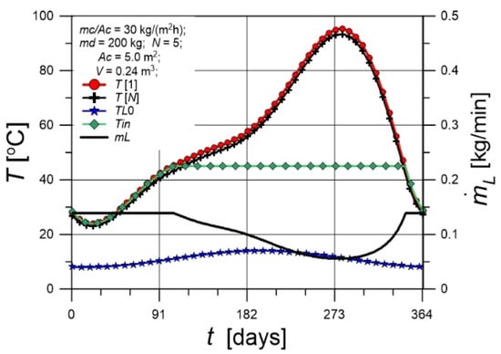
Figure 9.
Time courses of temperatures and of the flow rate in the solar water heating installation.
Figure 10 presents the daily heat quantities transferred within the solar water heating installation. The relative positions of the curves for Qu, Qd, and QL show that the solar energy delivered to the tank (Qu) is insufficient to raise the domestic hot water to the desired temperature. The algebraic sum of these heat quantities yields the curve representing the daily energy demand supplied by the auxiliary heating device. The auxiliary heat Qa must be provided during the winter period, with its maximum daily value occurring in January and February.
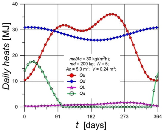
Figure 10.
Time courses of the daily heat quantities transferred in the solar water heating installation.
In Figure 11, the time courses of the dimensionless quantities characterizing the instantaneous performance of the process are presented. The instantaneous solar fraction Qs/Qd remains equal to its maximum value (equal to 1) for most of the year, indicating that auxiliary heating is not required during this period. Integration of this quantity over the entire year yields the annual solar fraction SF. The instantaneous solar efficiency takes values far from unity and is particularly low in late summer, when heat losses from the tank are highest and the inlet cold-water temperature reaches its maximum. The figure also shows the utilizability and the critical radiation level ITc, discussed in Section 4.2. Under the considered conditions, the average annual value of ϕ was approximately 0.6. The time course of ITc is shown for different values of N. As shown, the influence of stratification on ITc is minimal, which results in no noticeable effect on ϕ, and consequently, on Qu and the indicators SF and SE.
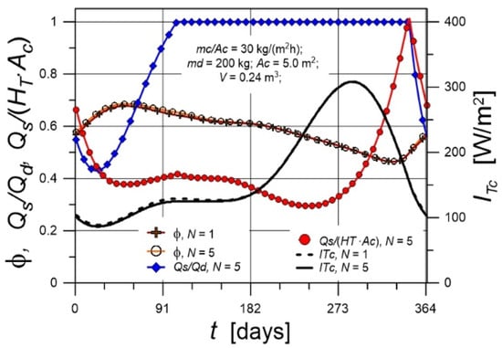
Figure 11.
Time courses of various heating-performance indicators and of the critical radiation level.
In Figure 12, the temperature profiles in the thermally stratified tank are presented. The results correspond to the autumn–winter period (days 307–349 of the year), during which the tank temperature decreases rapidly due to the depletion of energy accumulated during the summer. The calculations were carried out for N = 50. The temperature difference between the top and bottom of the tank reaches several degrees, with the largest temperature jump occurring at the last node. As the temperatures in the tank decrease, the profiles gradually become more uniform.
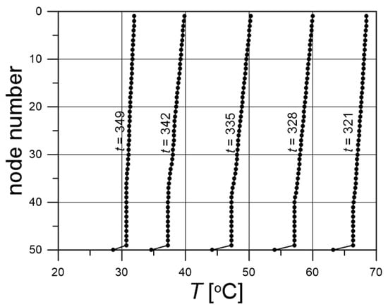
Figure 12.
Temperature profiles in the stratified tank for N = 50.
In Figure 13, the evolution of the temperature profiles in the tank is presented for N = 5.
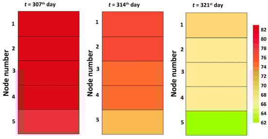
Figure 13.
Layered temperature profiles in the stratified tank for N = 5.
In Figure 14, the time-dependent changes in the locations at which the producing-loop stream enters the tank are presented, expressed as the node numbers i. These locations correspond to the arguments of the function Fc[i] for which Fc[i] = 1. The node numbers were determined according to the flowchart given in Appendix B. The plot covers the autumn–winter period (November–January), during which the temperature of the water supplied from the collectors to the tank varied rapidly. Calculations were performed for several combinations of tank volume V and mass flow rate in the producing loop, . A value of N = 5 was assumed, corresponding to five possible inlet locations. During the spring–summer season, the collector stream enters node 1. As the inlet temperature decreases over time, the inlet is switched to node 2 and subsequently to node 3 or 4. Later in the season, the flow returns to nodes 3, 2, and finally 1. The smaller the tank volume, the higher the inlet temperature, and therefore the shorter the period during which the stream enters nodes with i > 1.
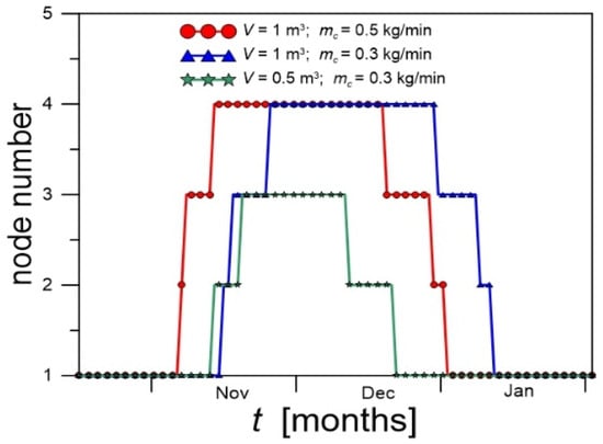
Figure 14.
Graphical presentation of the changes in the locations at which hot water is introduced into the tank.
Figure 15 and Figure 16 present the influence of the operating parameters of the solar domestic hot-water system on the key performance indicators—the solar fraction SF and the energy efficiency SE. The dominant factor affecting these indicators is the area of the installed solar collectors. Figure 15 shows that SF increases with increasing Ac, while SE decreases. The effect of the degree of stratification on SF and SE is small. Both indicators are slightly higher for larger values of N, but this effect diminishes as Ac increases. Figure 16 presents the effect of tank volume on SF and SE. This influence is practically negligible, as demonstrated for various combinations of Ac and N. In the study by Araujo [10], a noticeable influence of thermal stratification on the solar fraction was reported. The source of this discrepancy may lie in both the different models used in the calculations and the differing climatic conditions under which the simulations were performed.
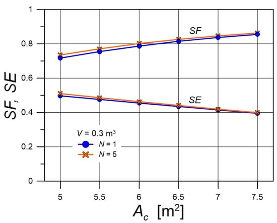
Figure 15.
The influence of collector area Ac and parameter N on the performance indicators SF and SE of the solar water heating process.
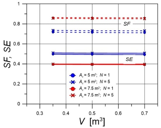
Figure 16.
The effect of tank volume V on the performance indicators SF and SE for various operating conditions of the solar water heating process.
6. Conclusions
Calculations focused on thermal stratification in a water storage tank were performed. The analysis was based on a multi-node model. A long-term (annual) operating period was considered, during which the tank was supplied with solar energy. Useful energy was evaluated using approximated climatic data derived from real measurements for Kraków, Poland. The objective of the study was to assess the influence of thermal stratification on the performance of solar water heating systems. The effects of water flow with variable temperature through a stratified tank were also investigated. Based on the performed calculations, it was found that:
- Incorporating the degree of stratification through the multi-node model does not pose computational difficulty, even though it requires solving a system of differential equations whose size equals the number of nodes. The system can be solved straightforwardly using standard numerical methods. Moreover, increasing the number of nodes beyond N = 10 is unnecessary, as it does not lead to meaningful changes in the results.
- No influence of the degree of stratification on process performance was observed for typical domestic hot-water conditions. In the design of small-scale solar systems, simplified heating models based on the assumption of perfect mixing in the tank should therefore be recommended.
- The collector area Ac has the dominant influence on performance indicators. The limitation is the maximum allowed water temperature in the tank, which may be exceeded when Ac becomes too large.
- It was demonstrated that the effect of thermal stratification in the storage tank on stabilizing the temperature of the water produced by the system is more significant than the effect resulting from increasing the tank volume.
- The degree of stratification plays an important role on the short-term (daily) scale. During the autumn–winter period, strong thermal stratification prevents temporary drops in DHW temperature when the tank volume is not sufficiently large. The numerical results show that stratification has a significant effect on stabilizing the outlet temperature when the inlet conditions vary over time.
Author Contributions
Conceptualization, K.K.; methodology, K.K. and B.K.; software, K.K. and B.K.; validation, K.K. and B.K.; formal analysis, K.K.; investigation, K.K. and B.K.; data curation, K.K. and B.K.; writing—original draft preparation, K.K.; writing—review and editing, K.K. and B.K.; visualization, K.K. and B.K.; supervision, K.K. and B.K.; All authors have read and agreed to the published version of the manuscript.
Funding
This research received no external funding.
Data Availability Statement
Dataset available on request from the authors.
Conflicts of Interest
The authors declare no conflicts of interest.
Nomenclature
| A[i] | surface area of the tank (node), m2 |
| Ac | solar collectors’ surface area, m2 |
| c | heat capacity, J/(kgK) |
| Fc, FL | functions defined in the flowchart (Figure A1) |
| FR | collector heat removal factor |
| FR’ | modified collector heat removal factor |
| H | daily radiation on the horizontal surface, J/m2 |
| HT | daily radiation on a tilted surface, J/m2 |
| i | node number |
| init | initial value |
| ITc | critical radiation level, W/m2 |
| n | day of the year |
| N | number of nodes |
| water flow rate in the collector circuit, kg/s | |
| water flow rate in the consumption circuit, kg/s | |
| water flow rate in the by-pass, kg/s | |
| Md | the mass of DHW consumed daily, kg |
| M[i] | the mass of water in node i |
| Qa | daily heat from auxiliary source, J |
| Qd | the heat required to produce the daily amount of DHW, J |
| QL | daily tank heat losses, J |
| Qu | daily useful heat, J |
| SE | solar efficiency defined by Equation (25) |
| SF | solar fraction defined by Equation (24) |
| T | temperature, °C |
| Ta | air temperature, °C |
| Td | DHW temperature, °C |
| Tg | tank surroundings temperature, °C |
| Tin | reheaters’ inlet temperature, °C |
| Tc | production circuit temperature, °C |
| TL | consumption circuit temperature, °C |
| t | time |
| ∆t | time step (= 1 day) |
| Ut | overall heat transfer coefficient between the tank and the surroundings, W/(m2K) |
| V | volume of tank, m3 |
| (τα) | effective transmittance—absorptance product |
| β | collectors slope, rad or ° |
| ρ | water density, kg/m3 |
| ∑ | summing from 1 to 365 days |
| ϕ | daily utilizability |
| ψ | latitude, ° |
| Abbreviations | |
| CFD | Computational Fluid Dynamics |
| DHW | Domestic Hot Water |
| PCM | Phase Change Material |
| RND | Random Error Generator |
Appendix A. Heat Balances
Mixing node (balance area marked in cyan in Figure 7)
The mixed stream, leaving the flow mixer at temperature Tin, flows with the average rate . The mass and heat balances take the form:
Producing loop (balance area marked in yellow in Figure 7)
Water enters the collector at inlet temperature T[N] and leaves at temperature Tc0. The mass flow rate of water through the collector is , and over a day the water absorbs a useful heat quantity Qu. Thus:
Appendix B. Flowcharts
In Figure A1, the flowcharts for determining the values of the functions Fc and FL, which specify the inlet locations of the producing and consuming streams in the tank, are presented.

Figure A1.
Flowchart for determining the functions Fc and FL.
References
- Braun, J.E.; Klein, S.A.; Mitchell, J.W. Seasonal Storage of Energy in Solar Heating. Sol. Energy 1981, 26, 403–411. [Google Scholar] [CrossRef]
- Duffie, J.A.; Beckman, W.A. Solar Engineering of Thermal Processes; Wiley: Hoboken, NJ, USA, 2013. [Google Scholar] [CrossRef]
- Kalogirou, S.A. Solar Energy Engineering, 3rd ed.; Elsevier: Amsterdam, The Netherlands, 2023. [Google Scholar]
- Kleinbach, E.; Beckman, W.A.; Klein, S.A. Performance Study of One-Dimensional Models for Stratified Thermal Storage Tanks. Sol. Energy 1993, 50, 155–166. [Google Scholar] [CrossRef]
- Han, Y.; Wang, R.; Dai, Y. Thermal Stratification within the Water Tank. Renew. Sustain. Energy Rev. 2009, 13, 1014–1026. [Google Scholar] [CrossRef]
- Liu, B.; Gao, W.; Li, Q.; Chen, H.; Zhang, Y.; Ding, X. Quantification of Thermal Stratification and Its Impact on Energy Efficiency in Solar Hot Water Storage Tanks. Energy 2025, 326, 136243. [Google Scholar] [CrossRef]
- Rosen, M.A. The Exergy of Stratified Thermal Energy Storages. Sol. Energy 2001, 71, 173–185. [Google Scholar] [CrossRef]
- Rosen, M.A.; Tang, R.; Dincer, I. Effect of Stratification on Energy and Exergy Capacities in Thermal Storage Systems. Energy 2004, 29, 1115–1127. [Google Scholar] [CrossRef]
- Riebel, A.; Wolde, I.; Escobar, R.; Barraza, R.; Cardemil, J.M. Transient Modeling of Stratified Thermal Storage Tanks: Comparison of 1D Models and the Advanced Flowrate Distribution Method. Case Stud. Therm. Eng. 2024, 61, 105084. [Google Scholar] [CrossRef]
- Araújo, A.; Silva, R. Energy Modeling of Solar Water Heating Systems with On–Off Control and Thermally Stratified Storage Using a Fast Computation Algorithm. Renew. Energy 2020, 150, 891–906. [Google Scholar] [CrossRef]
- Andersen, E.; Furbo, S. Stratification Devices. In Proceedings of the Conference on Thermal Storage, Prague, Czech Republic, 13–14 March 2008. [Google Scholar]
- Andersen, E.; Furbo, S. Long-Time Durability Tests of Fabric Inlet Stratification Pipes. In Proceedings of the EuroSun 2008 Congress, Lisbon, Portugal, 7–10 October 2008. [Google Scholar]
- Wang, Z.; Zhang, H.; Huang, H.; Dou, B.; Huang, X.; Goula, M.A. Experimental Investigation of Thermal Stratification in a Solar Hot Water Tank. Renew. Energy 2019, 134, 862–874. [Google Scholar] [CrossRef]
- Cònsul, R.; Rodríguez, I.; Pérez-Segarra, C.D.; Soria, M. Virtual Prototyping of Storage Tanks by Means of Three-Dimensional CFD and Heat Transfer Simulations. Sol. Energy 2004, 77, 179–191. [Google Scholar] [CrossRef]
- Ievers, S.; Lin, W. Numerical Simulation of Three-Dimensional Flow Dynamics in a Hot Water Storage Tank. Appl. Energy 2009, 86, 2604–2614. [Google Scholar] [CrossRef]
- Yaïci, W.; Entchev, E.; Ghorab, M.; Hayden, A.C. Three-Dimensional Unsteady CFD Simulations of a Thermal Storage Tank Performance for Optimum Design. Appl. Therm. Eng. 2013, 60, 152–163. [Google Scholar] [CrossRef]
- Bouhal, T.; Fertahi, S.; Agrouaz, Y.; El Rhafiki, T.; Kousksou, T.; Jamil, A. Numerical Modeling and Optimization of Thermal Stratification in Solar Hot Water Storage Tanks for Domestic Applications: CFD Study. Sol. Energy 2017, 157, 441–455. [Google Scholar] [CrossRef]
- Kumar, K.; Singh, S. Investigating Thermal Stratification in a Vertical Hot Water Storage Tank under Multiple Transient Operations. Energy Rep. 2021, 7, 7186–7199. [Google Scholar] [CrossRef]
- Liu, B.; Gao, W.; Zhang, Y.; Ding, X.; Li, Q.; Wang, J. Effect of Initial Temperature of Water in a Solar Hot Water Storage Tank on Thermal Stratification under Discharging Mode. Renew. Energy 2023, 212, 994–1004. [Google Scholar] [CrossRef]
- Gómez, M.A.; Collazo, J.; Porteiro, J.; Míguez, J.L. Numerical Study of an External Device for Improving Thermal Stratification in Hot Water Storage Tanks. Appl. Therm. Eng. 2018, 144, 996–1009. [Google Scholar] [CrossRef]
- Kong, L.; Yuan, W.; Zhu, N. CFD Simulations of Thermal Stratification in a Heat-Storage Water Tank with an Inside Cylinder with Openings. Procedia Eng. 2016, 146, 394–399. [Google Scholar] [CrossRef]
- Abdidin, A.; Seitov, A.; Toleukhanov, A.; Belyayev, Y.; Botella, O.; Kheiri, A.; Khalij, M. Three-Dimensional CFD Analysis of a Hot Water Storage Tank with Various Inlet/Outlet Configurations. Energies 2024, 17, 5716. [Google Scholar] [CrossRef]
- Lou, W.; Luo, L.; Hua, Y.; Fan, Y.; Du, Z. A Review on Performance Indicators and Influencing Factors for Thermocline Thermal Energy Storage Systems. Energies 2021, 14, 8384. [Google Scholar] [CrossRef]
- Janus, J.; Filipowska, M.; Jabłoński, H.; Wieliński, M.; Sornek, K. Overview of Technologies for Solar Systems and Heat Storage: The Use of Computational Fluid Dynamics for Performance Analysis and Optimization. Energies 2024, 17, 6001. [Google Scholar] [CrossRef]
- Barrasso, M.; Langella, G.; Amoresano, A.; Iodice, P. Latest Advances in Thermal Energy Storage for Solar Plants. Processes 2023, 11, 1832. [Google Scholar] [CrossRef]
- Bai, Y.; Yang, M.; Fan, J.; Li, X.; Chen, L.; Yuan, G.; Wang, Z. Influence of Geometry on the Thermal Performance of Water Pit Seasonal Heat Storages for Solar District Heating. Build. Simul. 2021, 14, 579–599. [Google Scholar] [CrossRef]
- Smith, S.W. The Scientist and Engineer’s Guide to Digital Signal Processing, 2nd ed.; California Technical Publishing: San Diego, CA, USA, 1997. [Google Scholar]
- Photovoltaic Geographical Information System (PVGIS). Available online: https://joint-research-centre.ec.europa.eu/photovoltaic-geographical-information-system-pvgis_en (accessed on 3 December 2025).
- Kupiec, K.; Król, B. Optimal Collector Tilt Angle to Maximize Solar Fraction in Residential Heating Systems: A Numerical Study for Temperate Climates. Sustainability 2025, 17, 6385. [Google Scholar] [CrossRef]
- Kupiec, K.; Pater, S. On the Possibility of Achieving High Solar Fractions for Space Heating in Temperate Climates. Sol. Energy 2025, 300, 113789. [Google Scholar] [CrossRef]
- Chiasson, A.D. Geothermal Heat Pump and Heat Engine System; Wiley: Hoboken, NJ, USA, 2016. [Google Scholar]
Disclaimer/Publisher’s Note: The statements, opinions and data contained in all publications are solely those of the individual author(s) and contributor(s) and not of MDPI and/or the editor(s). MDPI and/or the editor(s) disclaim responsibility for any injury to people or property resulting from any ideas, methods, instructions or products referred to in the content. |
© 2026 by the authors. Licensee MDPI, Basel, Switzerland. This article is an open access article distributed under the terms and conditions of the Creative Commons Attribution (CC BY) license.