Dual-Agent Deep Reinforcement Learning for Low-Carbon Economic Dispatch in Wind-Integrated Microgrids Based on Carbon Emission Flow

Abstract

High renewable penetration in microgrids makes low-carbon economic dispatch under uncertainty challenging, and single-agent deep reinforcement learning (DRL) often yields unstable cost–emission trade-offs. This study proposes a dual-agent DRL framework that explicitly balances operational economy and environmental sustainability. A Proximal Policy Optimization (PPO) agent focuses on minimizing operating cost, while a Soft Actor–Critic (SAC) agent targets carbon emission reduction; their actions are combined through an adaptive weighting strategy. The framework is supported by carbon emission flow (CEF) theory, which enables network-level tracing of carbon flows, and a stepped carbon pricing mechanism that internalizes dynamic carbon costs. Demand response (DR) is incorporated to enhance operational flexibility. The dispatch problem is formulated as a Markov Decision Process, allowing the dual-agent system to learn policies through interaction with the environment. Case studies on a modified PJM 5-bus test system show that, compared with a Deep Deterministic Policy Gradient (DDPG) baseline, the proposed method reduces total operating cost, carbon emissions, and wind curtailment by 16.8%, 11.3%, and 15.2%, respectively. These results demonstrate that the proposed framework is an effective solution for economical and low-carbon operation in renewable-rich power systems.

1. Introduction

The accelerating global transition toward a low-carbon economy has become a critical pathway for mitigating climate change and achieving sustainable energy development. In this context, the integration of renewable energy resources into power grids has received significant attention. According to the World Energy Transitions Outlook by the International Renewable Energy Agency (IRENA), renewable energy is projected to account for approximately three-quarters of the global energy mix by 2050, while electricity will become the dominant energy carrier, meeting more than 50% of total energy consumption [1]. Microgrids, as decentralized and flexible energy systems, provide an effective platform for integrating renewable generation and enhancing the resilience, efficiency, and low-carbon characteristics of modern power networks [2]. However, the intermittency and uncertainty of renewable resources present substantial challenges, specifically regarding voltage violations caused by reverse power flow, frequency instability due to low inertia, and the difficulty of maintaining real-time power balance under extreme weather conditions.

To address the dual objectives of economic efficiency and emission reduction, extensive research has been conducted on low-carbon economic dispatch in integrated energy systems. In [3], a multi-energy microgrid optimization framework incorporating Power-to-Gas (P2G) and Carbon Capture and Storage (CCS) technologies was developed to improve system efficiency and reduce carbon emissions. Meanwhile, the role of carbon pricing and trading mechanisms in promoting emission reduction has been widely investigated [4]. Studies have shown that these mechanisms effectively internalize the environmental cost of power generation, thereby altering the dispatch merit order to favor lower-carbon sources over fossil-fuel-intensive ones. For example, stepwise carbon pricing schemes have been introduced to enhance the effectiveness of carbon emission constraints [5], while combined green certificate and carbon trading mechanisms have been proposed to promote low-carbon transitions in multi-regional systems [6], which demonstrated that a coupled market mechanism could reduce total system emissions by approximately 15% compared to independent trading markets. Nevertheless, these models often rely on deterministic assumptions and static formulations that fail to capture the stochastic and time-varying nature of renewable generation [7,8]. For instance, static optimization often relies on day-ahead forecasts with error margins exceeding 20%, leading to frequent real-time power imbalances that require costly redispatching.

With the rapid development of artificial intelligence, DRL has emerged as a promising paradigm for addressing complex, high-dimensional, and uncertain optimization problems in power systems. DRL enables adaptive decision-making by learning optimal operational strategies that balance multiple objectives, such as minimizing costs and reducing carbon emissions, under dynamic and uncertain environments [9]. For instance, Ref. [10] employed DRL with self-adaptive hyperparameter adjustment to achieve real-time multi-objective scheduling for multi-energy microgrids integrating post-carbon and direct-air carbon capture systems. Similarly, Ref. [11] utilized DRL to handle the uncertainty of wind and photovoltaic generation while optimizing system costs, network losses, and voltage stability indicators. Moreover, advanced DRL algorithms such as the Soft SAC [12] and PPO [13] have demonstrated superior stability and convergence performance in complex dispatch tasks. However, most existing DRL-based approaches are developed within a single-agent learning framework, which may lead to suboptimal results when dealing with multiple conflicting objectives, particularly in balancing economic operation and carbon emission mitigation.

To overcome these limitations, this paper proposes a dual-agent DRL framework for low-carbon economic dispatch in microgrids. The proposed framework integrates two cooperative agents, namely a PPO-based agent for economic optimization and an SAC-based agent for carbon emission minimization. Through coordinated learning and decision-making, the two agents effectively manage the trade-off between operational cost and emission reduction, providing a more robust and stable dispatch strategy compared with conventional single-agent approaches such as DDPG [14]. Furthermore, a DR mechanism [15] is incorporated to enhance system flexibility by enabling load adjustments in response to real-time carbon pricing signals, thereby improving the adaptability and overall efficiency of microgrid operations.

The main contributions of this study are summarized as follows. First, a novel dual-agent DRL architecture is developed to jointly optimize economic and carbon objectives, addressing the limitations of conventional single-agent DRL models. Second, a DSR mechanism is integrated into the framework to enhance operational flexibility and further improve economic and environmental performance. Finally, comprehensive case studies are conducted to validate the effectiveness of the proposed model, demonstrating superior performance over existing benchmark algorithms in terms of cost reduction, emission mitigation, and renewable energy utilization.

2. Carbon Emission Flow Theory Research

CEF is an innovative carbon emission analysis method that has been gradually applied and developed in power systems [15]. The core idea is to treat carbon emissions in a power system as a flowing process. By combining carbon emissions with power flow analysis, the CEF theory dynamically examines the distribution and flow of carbon emissions across various sectors. As shown in Figure 1, the carbon emission flow structure illustrates how emissions are traced from generation to consumption. This theory helps to reveal the specific sources of carbon emissions in the power production and consumption process, as well as quantify the contribution of each sector.

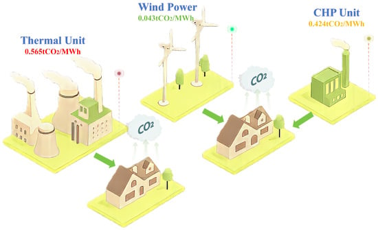
Figure 1. Carbon emission flow structure.

2.1. Basic Concepts of Carbon Emission Flow in Power Systems

In power systems, the primary source of carbon emissions comes from power generation, and different generation technologies have distinct carbon emission characteristics. Therefore, carbon emission flow is not just a byproduct of electricity production but is closely related to power flow, forming a new analytical tool. Through carbon emission flow analysis, we can obtain indicators such as carbon flow, carbon flow rate, and carbon flow density on each branch, reflecting the distribution and transmission of carbon emissions in the power system.

The carbon flow on a branch refers to the total amount of carbon emissions passing through a branch of the power system within a unit of time. It can be calculated using the following formula:

$$F_s={\int }_{t_1}^{t_2}{R}_{s}dt$$

(1)

where $F_s$ represents the carbon flow on branch s, and $R_s$ is the carbon flow rate on branch s, usually measured in ${\mathrm{tCO}}_2/\mathrm{h}$.

The carbon flow rate represents the carbon flow per unit of time through a branch and is generally associated with the active power flow. It can be calculated as:

$$R_s={\displaystyle \frac{d{F}_s}{dt}}$$

(2)

where $R_s$ is the carbon flow rate, measured in ${\mathrm{tCO}}_2/\mathrm{h}$ or ${\mathrm{kgCO}}_2/\mathrm{s}$. The carbon flow rate dynamically reflects the carbon emission situation at different time points in the power system.

2.2. Carbon Flow Density and Its Relationship with Power Flow

One of the key characteristics of carbon emission flow is its close relationship with power flow. Carbon flow density is defined as the ratio of the carbon flow rate to the active power flow on a branch [16]:

$$\rho ={\displaystyle \frac{R_s}{P_s}}$$

(3)

where $R_s$ is the carbon flow rate on branch s and $P_s$ is the active power flow on branch s. This formula reveals the relationship between the carbon flow density and power flow, reflecting the transmission process of carbon emissions in the power system.

2.3. Node Carbon Potential

Node carbon potential refers to the carbon emission intensity at a particular node in the power system, indicating the amount of carbon emissions generated per unit of electricity consumed at that node [16]. The node carbon potential can be calculated as:

$$e_{nj}={\displaystyle \frac{{\sum }_{s\in L_j^{+}}{P}_s·{\rho }_s}{{\sum }_{s\in L_j^{+}}{P}_s}}$$

(4)

where $e_{nj}$ represents the carbon potential at node j, $P_s$ is the power flow on branch s, ${\rho }_s$ is the carbon flow density on branch s, and $L_j^{+}$ is the set of branches connected to node j.

3. Generator Carbon Emission Calculation Model

In modern low-carbon power system scheduling, carbon emission calculation and the stepwise carbon pricing calculation model play a critical role [17]. By accurately quantifying carbon emissions and associated carbon costs, these models provide a foundation for optimizing scheduling strategies and enable the rational pricing of carbon emissions within the system.

Therefore, a dynamic carbon emission calculation model has been proposed. This model divides the generator’s output into several different intervals, with the number of intervals increasing as the output power increases. The carbon emission intensity in each interval gradually stabilizes. The carbon emission of each generator at a specific time is calculated by first determining the output in each interval and combining it with the carbon emission intensity of that interval. The total carbon emission is then obtained by summing the emissions from all intervals. The model is expressed as follows:

$$B(i,t)=\left\{\begin{array}{c}{\psi }_1[P(i,t)-P_0],\hfill \\ min(P_{\min },P_0)\le P(i,t)<P_0+p\hfill \\ {\psi }_1[P(i,t)-P_0]+{\psi }_1[P(i,t)-P_0]{\xi }_1,\hfill \\ P_0+p\le P(i,t)<P_0+2p\hfill \\ {\psi }_1[P(i,t)-P_0]+{\psi }_1[P(i,t)-P_0]{\xi }_2,\hfill \\ P_0+2p\le P(i,t)<P_0+3p\hfill \\ ⋮\hfill & \\ {\psi }_1[P(i,t)-P_0]+\dots +{\psi }_1[P(i,t)-P_0]{\xi }_n,\hfill \\ P_0+(n-1)p\le P(i,t)<min(P_0+np,P_{\max })\hfill \end{array}\right.$$

(5)

where $B(i,t)$ represents the total carbon emissions of unit i at time t; $P(i,t)$ is the power output of unit i at time t; $P_0$ is the minimum power output of the unit; $P_{\min }$ and $P_{\max }$ represent the minimum and maximum power outputs of the unit, respectively; p is the interval length; ${\xi }_1,{\xi }_2,\dots ,{\xi }_n$ are the increment factors for the corresponding intervals, which increase as the carbon emission intensity increases.

To effectively reduce peak carbon emissions, the carbon emission at each moment is divided into several different intervals. These intervals are associated with different costs, including low-carbon, mid-carbon, and high-carbon intervals. As the carbon emissions increase, the pricing for each interval gradually rises. The total carbon emission cost is calculated by summing the carbon emission of each interval multiplied by the corresponding carbon emission cost. The stepwise carbon pricing model is defined as:

$$C_{\mathrm{emi},i,t}=\left\{\begin{array}{c}{\psi }_2[B(i,t)-B_c],\hfill \\ B(i,t)<B_c+b\hfill \\ {\psi }_2[B(i,t)-B_c]+{\psi }_2[B(i,t)-B_c-b]\omega ,\hfill \\ B_c+b\le B(i,t)<B_c+2b\hfill \\ {\psi }_2[B(i,t)-B_c]+{\psi }_2[B(i,t)-B_c-b]\omega +{\psi }_2[B(i,t)-B_c-2b]\omega ,\hfill \\ B_c+2b\le B(i,t)<B_c+3b\hfill \\ ⋮\hfill & \end{array}\right.$$

(6)

where $C_{\mathrm{emi},i,t}$ represents the carbon emission cost of unit i at time t; ${\psi }_2$ is the base value of carbon emission cost; $B_c$ is the standard carbon emission value for the unit; b is the interval width; $\omega$ is the cost factor for the interval. In this study, $B_c=3000{\mathrm{tCO}}_2$ and $b=1000{\mathrm{tCO}}_2$, with the base carbon price set to ${\psi }_2=30\$/{\mathrm{tCO}}_2$ and the step growth factor set to $\omega =1.2$, selected to represent a typical daily cumulative emission level of the PJM-5 benchmark and to ensure a stable yet sufficiently discriminative tier transition. As the carbon emissions increase, the cost increases gradually.

4. Problem Formulation

As shown in Figure 2, the microgrid dispatch process is formulated as an agent–environment interaction in the reinforcement learning paradigm. At each time step, the agent observes the system state (e.g., load demand, wind power forecasts, previous dispatch decisions, and carbon-related indicators), determines dispatch actions for thermal generation, demand response, and wind utilization, and then receives a reward that reflects the trade-off between operating cost, carbon emissions, and renewable energy accommodation. This closed-loop interaction enables the agent to iteratively improve its policy through trial-and-error learning under uncertainty.

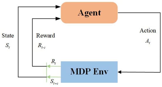
Figure 2. Agent–Environment interaction.

4.1. Optimization Model

4.1.1. Objective Function

The multi-objective optimization problem for low-carbon economic dispatch in microgrids aims to minimize the total system operating cost, which comprehensively considers power generation costs, carbon emission costs, and demand response costs. The mathematical formulation is expressed as:

$$min\sum _{t=1}^T\left[C_{\mathrm{gen}}\left(t\right)+C_{\mathrm{carbon}}\left(t\right)+C_{\mathrm{dr}}\left(t\right)\right]$$

(7)

where $C_{\mathrm{gen}}\left(t\right)$ represents the total power generation cost at time t, $C_{\mathrm{carbon}}\left(t\right)$ denotes the total carbon emission cost at time t, calculated using the stepped carbon pricing mechanism, $C_{\mathrm{dr}}\left(t\right)$ indicates the demand response cost at time t, and T is the dispatch period (24 h).

4.1.2. Detailed Cost Component Modeling

Power Generation Cost Function:

$$C_{\mathrm{gen}}\left(t\right)=\sum _{i=1}^{N_g}{C}_{g,i}\left(t\right)+\sum _{j=1}^{N_w}{C}_{w,j}\left(t\right)$$

(8)

where $N_g$ is the number of thermal power units, $N_w$ is the number of wind power units, $C_{g,i}\left(t\right)$ represents the generation cost of the i-th thermal unit at time t, and $C_{w,j}\left(t\right)$ represents the generation cost of the j-th wind unit at time t.

Thermal Unit Cost Model:

$$C_{g,i}\left(t\right)=a_i·P_{g,i}^2\left(t\right)+b_i·P_{g,i}\left(t\right)+c_i$$

(9)

where $a_i,b_i,c_i$ are the cost coefficients of the i-th thermal unit, and $P_{g,i}\left(t\right)$ is the output power of the i-th thermal unit at time t.

Wind Unit Cost Model:

$$C_{w,j}\left(t\right)=k_w·P_{w,j}\left(t\right)$$

(10)

where $k_w$ is the wind power generation cost coefficient, and $P_{w,j}\left(t\right)$ is the output power of the j-th wind unit at time t.

4.1.3. Carbon Emission Cost Model

The carbon emission cost is calculated using the stepped carbon pricing mechanism defined in Section 3:

$$C_{\mathrm{carbon}}\left(t\right)=\sum _{i=1}^{N_g}{C}_{\mathrm{emi},i,t}$$

(11)

4.1.4. Demand Response Cost Model

$$C_{\mathrm{dr}}\left(t\right)=\sum _{m=1}^{N_{\mathrm{dr}}}{\lambda }_m\left(t\right)·\left|P_{\mathrm{dr},m}\left(t\right)\right|$$

(12)

where $N_{\mathrm{dr}}$ is the number of load nodes participating in demand response, ${\lambda }_m\left(t\right)$ is the load transfer cost coefficient of node m at time t, and $P_{\mathrm{dr},m}\left(t\right)$ is the load transfer power of node m at time t.

4.2. Markov Decision Process Modeling

4.2.1. State Space Definition

The microgrid dispatch problem is formulated as a Markov Decision Process with the following state vector [18]:

$$\begin{array}{cc}\hfill s_t=& \left[{\tilde{P}}_L\left(t\right),{\tilde{P}}_W^{\mathrm{forecast}}\left(t\right),{\tilde{P}}_L^{\mathrm{forecast}}(t+1),{\tilde{P}}_W^{\mathrm{forecast}}(t+1),{\tilde{P}}_G(t-1),\right.\hfill \\ \hfill & {\left.{\tilde{P}}_W(t-1),\tau \left(t\right),d\left(t\right),{\tilde{B}}_{\mathrm{cum}}\left(t\right),{\tilde{U}}_{\mathrm{cum}}\left(t\right),{\tilde{\mathbf{e}}}_n\left(t\right)\right]}^T\hfill \end{array}$$

(13)

The components are defined as follows: ${\tilde{P}}_L\left(t\right)$: normalized nodal load vector at time t; ${\tilde{P}}_W^{\mathrm{forecast}}\left(t\right)$: normalized wind power forecast vector at time t; ${\tilde{P}}_L^{\mathrm{forecast}}(t+1)$: one-step-ahead forecasts of load; ${\tilde{P}}_W^{\mathrm{forecast}}(t+1)$: one-step-ahead forecasts of wind power; ${\tilde{P}}_G(t-1)$: normalized outputs of thermal units at the previous time step; ${\tilde{P}}_W(t-1)$: normalized outputs of dispatched wind power at the previous time step; $\tau \left(t\right)$: normalized time index, $d\left(t\right)$: demand-response indicator (donor, receiver, or non-DR period); ${\tilde{B}}_{\mathrm{cum}}\left(t\right)$: cumulative carbon emission vector up to time t; ${\tilde{U}}_{\mathrm{cum}}\left(t\right)$: cumulative wind curtailment vectors up to time t; and ${\tilde{\mathbf{e}}}_n\left(t\right)$: the normalized node carbon potential vector calculated via CEF theory at time t. Here, the tilde “∼” denotes that the corresponding quantity is normalized.

4.2.2. Action Space Design

The action space comprises continuous decision variables:

$$a_t=\left[P_G\left(t\right),P_{dr}\left(t\right),a_W\left(t\right)\right]$$

(14)

where $P_G\left(t\right)\in {\mathbb{R}}^{N_g}$: dispatch decision vector for thermal units; $P_{dr}\left(t\right)\in {\mathbb{R}}^{N_{dr}}$: load transfer power decision vector; and $a_W\left(t\right)\in {[0,1]}^{N_w}$: wind power utilization decision vector.

4.2.3. Reward Function Design

A multi-objective reward function is designed to balance economic efficiency and low-carbon performance:

$$R(s_t,a_t)=w_1{R}_{\mathrm{economic}}+w_2{R}_{\mathrm{carbon}}+w_3{R}_{\mathrm{renewable}}$$

(15)

Economic Reward:

$$R_{\mathrm{economic}}=-{\displaystyle \frac{C_{\mathrm{total}}\left(t\right)}{C_{\mathrm{norm}}}}$$

(16)

where $C_{\mathrm{total}}\left(t\right)=C_{\mathrm{gen}}\left(t\right)+C_{\mathrm{carbon}}\left(t\right)+C_{\mathrm{dr}}\left(t\right)$ and $C_{\mathrm{norm}}$ is the cost normalization coefficient.

Low-carbon Reward:

$$R_{\mathrm{carbon}}=-{\displaystyle \frac{{\sum }_{i=1}^{N_g}{B}_{g,i}\left(t\right)}{B_{\mathrm{norm}}}}$$

(17)

Renewable Energy Utilization Reward:

$$R_{\mathrm{renewable}}={\displaystyle \frac{{\sum }_{j=1}^{N_w}{p}_{w,j}\left(t\right)}{{\sum }_{j=1}^{N_w}{p}_{\mathrm{forecast},w,j}\left(t\right)}}$$

(18)

The weight coefficients satisfy $w_1+w_2+w_3=1$ and are dynamically adjusted according to dispatch objectives.

Note that this global reward is used as an overall evaluation metric to quantify the Pareto trade-off, while the two agents are trained with objective-specific rewards.

4.3. System Operational Constraints

4.3.1. Power Balance Constraint

$$\sum _{i=1}^{N_g}{P}_{g,i}\left(t\right)+\sum _{j=1}^{N_w}{P}_{w,j}\left(t\right)=\sum _{n=1}^N{P}_{L,n}\left(t\right)+\sum _{m=1}^{N_{dr}}{P}_{dr,m}\left(t\right)$$

(19)

4.3.2. Generator Operational Constraints

Output Power Limits:

$$P_{g,i}^{\min }\le P_{g,i}\left(t\right)\le P_{g,i}^{\max },\forall i\in [1,N_g],\forall t\in [1,T]$$

(20)

$$0\le P_{w,j}\left(t\right)\le P_{w,j}^{\mathrm{forecast}}\left(t\right),\forall j\in [1,N_w],\forall t\in [1,T]$$

(21)

Ramp Rate Constraints:

$$-R_{g,i}^{\mathrm{down}}\le P_{g,i}\left(t\right)-P_{g,i}(t-1)\le R_{g,i}^{\mathrm{up}},\forall i\in [1,N_g],\forall t\in [2,T]$$

(22)

4.3.3. Demand Response Constraints

Capacity Constraints:

$$|P_{dr,m}\left(t\right)|\le P_{dr,m}^{\max },\forall m\in [1,N_{dr}],\forall t\in [1,T]$$

(23)

Time Period Constraints:

$$P_{dr,m}\left(t\right)\le 0,\forall t\in T_{\mathrm{donor}}$$

(24)

$$P_{dr,m}\left(t\right)\ge 0,\forall t\in T_{\mathrm{receiver}}$$

(25)

where $T_{\mathrm{donor}}$ and $T_{\mathrm{receiver}}$ represent load reduction periods and load recovery periods, respectively.

4.3.4. Network Security Constraints

Line Power Flow Constraints:

$$|P_l\left(t\right)|\le P_l^{\max },\forall l\in [1,L],\forall t\in [1,T]$$

(26)

Node Voltage Constraints:

$$V_n^{\min }\le V_n\left(t\right)\le V_n^{\max },\forall n\in [1,N],\forall t\in [1,T]$$

(27)

This optimization problem constitutes a high-dimensional, nonlinear, multi-timescale complex constrained optimization problem that is challenging to solve effectively using traditional optimization methods, thus motivating the adoption of a deep reinforcement learning framework for solution.

5. Solving Low-Carbon Dispatch Model Based on Dual-Agent

5.1. PPO for Economic Dispatch

The PPO algorithm is a model-free reinforcement learning method that optimizes a surrogate objective function based on the policy gradient approach. PPO has demonstrated robustness in training deep reinforcement learning models, offering a more stable alternative to conventional policy optimization techniques, such as TRPO (Trust Region Policy Optimization). In the context of economic dispatch, the objective is to minimize the operating costs of the microgrid system, which involves reducing generation costs, wind curtailment penalties, and carbon-related costs [19].

The PPO algorithm operates by optimizing the following objective function, defined at each time step t:

$$L\left(\theta \right)={\mathbb{E}}_t\left[min\left(r_t\left(\theta \right){\widehat{A}}_t,\mathrm{clip}(r_t\left(\theta \right),1-ϵ,1+ϵ){\widehat{A}}_t\right)\right]$$

(28)

where:

(a) $r_t\left(\theta \right)$ is the probability ratio of the new and old policies:

$$r_t\left(\theta \right)={\displaystyle \frac{{\pi }_{\theta }\left(a_t\right|s_t)}{{\pi }_{{\theta }_{\mathrm{old}}}\left(a_t\right|s_t)}}$$

(29)

Here, ${\pi }_{\theta }\left(a_t\right|s_t)$ represents the current policy, and ${\pi }_{{\theta }_{\mathrm{old}}}\left(a_t\right|s_t)$ is the previous policy.

(b) ${\widehat{A}}_t$ is the advantage function, which estimates the relative value of taking action $a_t$ in state $s_t$ compared to the baseline (value function):

$${\widehat{A}}_t=R_t-V_{\theta }\left(s_t\right)$$

(30)

where $R_t$ is the actual return observed after taking action $a_t$, and $V_{\theta }\left(s_t\right)$ is the state value function, which represents the expected return starting from state $s_t$.

(c) The clip operation is a critical component in PPO, ensuring that large policy updates are constrained, which helps maintain stable learning:

$$\mathrm{clip}(r_t\left(\theta \right),1-ϵ,1+ϵ)$$

(31)

where $ϵ$ is a hyperparameter that controls the magnitude of the policy update, typically set between 0.1 and 0.3.

The PPO objective function ensures that the policy is updated in a stable manner by limiting the variance of the policy gradient. The update is performed iteratively, utilizing stochastic gradient ascent to maximize the expected cumulative reward, defined over the states and actions taken by the policy.

The reward in this context is associated with the economic objectives, such as minimizing the total generation cost, curtailment cost, and carbon penalties. These rewards can be expressed as:

$$R_{\mathrm{economic}}=-C_{\mathrm{total}}=-(C_{\mathrm{thermal}}+C_{\mathrm{wind}}+C_{\mathrm{curtailment}}+C_{\mathrm{dr}}+C_{\mathrm{carbon}})$$

(32)

where $C_{\mathrm{thermal}}$ is the cost associated with thermal power generation, $C_{\mathrm{wind}}$ is the cost related to wind power generation, including curtailment penalties, $C_{\mathrm{curtailment}}$ penalizes wind curtailment, $C_{\mathrm{dr}}$ reflects the cost associated with demand response programs, and $C_{\mathrm{carbon}}$ accounts for carbon emissions from thermal generation.

5.2. SAC for Low-Carbon Dispatch

The SAC algorithm is an off-policy, model-free reinforcement learning approach designed to optimize continuous action spaces. SAC incorporates the principle of entropy regularization, which encourages exploration and stabilizes the training process by maximizing the entropy of the policy. This is particularly advantageous in scenarios with high uncertainty and multiple local optima, such as low-carbon dispatch in microgrids [20].

In SAC, the objective is to minimize the carbon emissions and wind curtailment while maximizing the utilization of renewable energy sources. The SAC algorithm optimizes the following objective function, where the agent learns to maximize the expected cumulative soft Q-value and the policy entropy:

$$J\left(\theta \right)={\mathbb{E}}_t\left[Q_{\varphi }(s_t,a_t)-\alpha log{\pi }_{\theta }\left(a_t\right|s_t)\right]$$

(33)

where $Q_{\varphi }(s_t,a_t)$ is the Q-function, which represents the expected return from taking action $a_t$ in state $s_t$, ${\pi }_{\theta }\left(a_t\right|s_t)$ is the policy function, which defines the probability distribution over actions, $\alpha$ is the temperature parameter, controlling the balance between exploration and exploitation by adjusting the entropy term $H\left({\pi }_{\theta }\right)$, and $H\left({\pi }_{\theta }\right)$ is the entropy of the policy, which measures the uncertainty in the actions taken by the agent.

The SAC algorithm aims to jointly maximize the soft Q-value and the entropy of the policy, thereby encouraging sufficient exploration while improving performance. This is achieved by solving the following Bellman equation:

$$Q_{\varphi }(s_t,a_t)=r_t+\gamma ·{\mathbb{E}}_{a_{t+1}\sim {\pi }_{\theta }}\left[Q_{\varphi }(s_{t+1},a_{t+1})-\alpha log{\pi }_{\theta }\left(a_{t+1}\right|s_{t+1})\right]$$

(34)

where $r_t$ is the immediate reward at time step t, and $\gamma$ is the discount factor that determines the importance of future rewards.

The soft Bellman backup is used to update the Q-values, and the policy update is done by maximizing the expected Q-values over all possible actions, adjusted by the entropy term.

The reward for the SAC agent is designed to penalize carbon emissions and curtailment while encouraging the maximization of renewable energy use. The low-carbon reward is given by:

$$R_{\mathrm{low}-\mathrm{carbon}}=-(\mathrm{carbon}\mathrm{penalties}+\mathrm{curtailment}\mathrm{penalties})$$

(35)

where carbon penalties are calculated based on the carbon emission associated with thermal generation, and curtailment penalties reflect the loss of renewable energy due to curtailment.

5.3. Dual-Agent Coordination and Action Fusion Strategy

To achieve the optimal balance between economic dispatch and low-carbon objectives, a dual-agent system is implemented. The final control action $a_{\mathrm{fused}}$ is obtained by combining the actions of the PPO and SAC agents through a weighted sum:

$$a_{\mathrm{fused}}=\alpha ·a_{\mathrm{PPO}}+\beta ·a_{\mathrm{SAC}}$$

(36)

where $\alpha$ and $\beta$ are the dynamic weights assigned to each agent, which reflect the relative importance of economic and low-carbon objectives. These weights are adjusted throughout the training process to achieve an optimal trade-off between the two conflicting goals. As shown in Figure 3, the overall dual-agent architecture and the action-fusion process are illustrated, highlighting how the two agents cooperate to balance economic and low-carbon objectives.

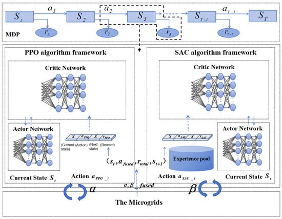
Figure 3. Dual-Agent system algorithm structure.

Since the economic and environmental objectives are inherently conflicting, a single global optimum may not exist. Instead, the proposed framework seeks a Pareto-optimal solution. The weighting factors $\alpha$ and $\beta$ in Equation (36) serve as dynamic negotiation coefficients, allowing the system to trade off marginal costs against marginal emission reductions, thereby preventing the policy from collapsing into extreme local optima (e.g., zero emissions with excessive load shedding). This weighted combination ensures that both economic and environmental considerations are addressed simultaneously, and the system can adaptively balance the emphasis on each goal based on the real-time performance of the microgrid.

6. Simulation Analysis

This study examines the impact of stepped carbon pricing and low-carbon dispatch mechanisms on source–load coordination through an intraday scheduling case study of a wind–thermal–demand response (DR) microgrid. The simulation is carried out on the PJM 5-bus test system [21], with the wind generation unit connected to bus E, as shown in Figure 4.

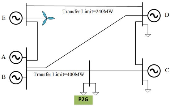
Figure 4. PJM-5-bus system.

The simulation spans a 24-h horizon with a 1-h resolution. Figure 5 shows the day-ahead forecasts of wind power (0–700 MW) and load (400–1000 MW). Wind generation is relatively high during 00:00–07:00, 12:00–15:00, and 21:00–23:00, but lower during 08:00–11:00 and 16:00–20:00. The load remains high between 07:00 and 20:00 and, except for 03:00–05:00, consistently exceeds wind generation.

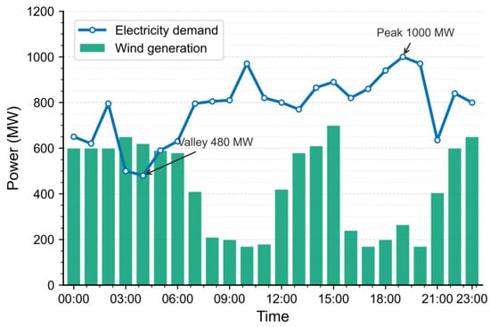
Figure 5. Wind Generation and Electricity Demand.

Table 1 summarizes the generator parameters for each bus. Carbon emissions are quantified using life-cycle assessment (LCA) coefficients, with 0.565 t/MWh assigned to coal-fired units. A stepped carbon-pricing scheme is employed in the carbon trading mechanism. The unit operating costs are specified as $4.2/MWh for thermal generation and $1.4/MWh for wind generation.

Table 1. Generator Parameters of the PJM 5-bus System.

Bus	Unit Type	Max Output (MW)	Bid Price ($/MWh)	Carbon Emission Factor (t/MWh)
A	Thermal Unit	110	14	0.565
B	Thermal Unit	100	15	0.565
C	CHP Unit	520	30	0.424
D	CHP Unit	200	35	0.424
E	Wind Power	700	10	0.043

Table values are based on the PJM 5-bus test system.

To evaluate the proposed dispatch method, the DDPG algorithm is adopted as the baseline [22]. While DDPG provides a representative single-agent baseline for continuous-action dispatch, it is acknowledged that the present comparison is limited and does not yet include PPO-only, SAC-only, or classical multi-objective optimization baselines. Extending the benchmark set to include these methods (e.g., single-agent PPO/SAC and traditional multi-objective optimization approaches) will be part of our future work to further validate the generality and competitiveness of the proposed framework. For comparative analysis, a dual-agent framework is constructed, combining PPO for the economic objective with SAC for the low-carbon objective. The parameter settings are summarized in Table 2, including learning rates and batch sizes, were selected based on a grid-search performance analysis. For instance, actor learning rates were tested in the range of ${10}^{-3}$, ${10}^{-4}$, and ${10}^{-5}$, with $2\times {10}^{-4}$ yielding the most stable convergence. To assess robustness, we repeat each method with 5 independent runs, Compared with single-agent approaches that often struggle with the conflicting gradients of economic and environmental rewards, the proposed Dual-Agent framework demonstrates higher robustness, maintaining lower variance in reward convergence across 5 independent training runs.

Table 2. Hyperparameters of DDPG and Dual-Agent.

Parameter	DDPG	Dual-Agent (PPO + SAC)
Replay Buffer Capacity	50,000	50,000
Discount Factor	0.95	0.95
Batch Size	64	PPO: 64/SAC: 256
Training Episodes	1000	1000
Soft Update Factor	0.0001	0.005
Actor Learning Rate	0.0002	PPO: 0.0002/SAC: 0.0002
Critic Learning Rate	0.0002	PPO: 0.0002/SAC: 0.0002

Comparisons of the pre- and post-DR load profiles and wind-power outputs obtained from DDPG and the Dual-Agent framework are shown in Figure 6. As illustrated in Figure 6a,b, during the evening peak (18:00–22:00), the post-DR curve under DDPG retains pronounced spikes, whereas the Dual-Agent leaves only minor residual peaks. In the early-morning valley (02:00–06:00), DDPG exhibits sharp hour-to-hour oscillations, while the Dual-Agent achieves more restrained and continuous valley filling. This improvement stems from goal decomposition with $\alpha$–$\beta$ decision fusion. PPO captures the economic policy by considering cost minimization, curtailment penalties, and stepped carbon pricing, while SAC focuses on the low-carbon policy of reducing emissions and curtailment. Their fused actions mitigate conflicts between objectives and suppress policy jitter, leading to temporally stable load reshaping. As a result, the Dual-Agent achieves a smaller peak-to-valley amplitude and smoother hour-to-hour transitions, demonstrating a more typical “peak shaving and valley filling” effect.

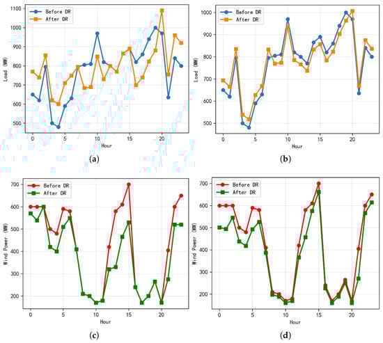
Figure 6. Simulation Results of the two Models: (a) Load Comparison Before/After DR by DDPG. (b) Load Comparison Before/After DR by Dual-Agent. (c) Wind Output Before/After DR by DDPG. (d) Wind Output Before/After DR by Dual-Agent.

Figure 6c,d show that, for the Dual-Agent, the pre- and post-DR wind outputs almost coincide, with deviations appearing only in capped deep valleys. This outcome reflects reduced curtailment and more continuous grid integration. Therefore, the Dual-Agent demonstrates superior performance in coordinating wind accommodation, load shifting, and thermal generation, making it better suited for dispatch under high renewable penetration.

Table 3 presents the comparative analysis of the two methods’ operating cost, carbon emissions, and wind curtailment after the implementation of DR. The Dual-Agent method outperforms DDPG across all three metrics. Specifically, the operating cost decreases from $422,867 to $351,894, carbon emissions decrease from 3978.0 t to 3526.9 t, and curtailment decreases from 1657.0 MWh to 1403.6 MWh. These improvements arise from goal decomposition with $\alpha$–$\beta$ weighted fusion. PPO optimizes the economic objective, while SAC targets the low-carbon and renewable-accommodation objective, thereby reducing conflicts inherent in a single value function. Magnitude-capped DR shifts demand toward wind-rich hours and prevents overcompensation. Thermal generation is coordinated more smoothly under ramp-rate and minimum-output constraints, which increases headroom for wind integration. The cost function also incorporates explicit carbon charges and curtailment penalties, steering the policy toward greater wind utilization. Consequently, the Dual-Agent delivers a more economical, cleaner, and more stable dispatch than the DDPG method.

Table 3. Comparison of Metrics between DDPG and Dual-Agent.

Metric	DDPG (Baseline)	Dual-Agent (PPO + SAC)
Cost ($)	422,867	351,894
Carbon (t)	3978.0	3526.9
Curtailment (MWh)	1657.0	1403.6

As shown in Table 3, the proposed method reduces the total operating cost by 16.8% and carbon emissions by 11.3% compared to the DDPG baseline. These improvements are significant when viewed against similar studies. For example, ref. [8] reported a cost reduction of approximately 9.5% using a single-agent DRL approach in a similar microgrid setup, suggesting that our collaborative dual-agent architecture unlocks further efficiency gains. Additionally, the wind curtailment reduction of 15.2% exceeds the typical range of 8–12% noted in recent reviews of microgrid dispatch strategies [7]. This superior performance demonstrates that decoupling the economic and low-carbon objectives into separate agents allows for more specialized and effective policy learning.

Although providing a strict convergence proof for deep reinforcement learning in continuous action spaces is beyond the scope of this work, we provide empirical evidence of training stability using logged optimization metrics. Specifically, Figure 7 reports the training evolution of two key objectives—total carbon emissions and total operating cost—versus episode for both the DDPG baseline and the proposed Dual-Agent framework. As training progresses, both metrics exhibit a clear stabilization trend, indicating that the learned policies converge to a steady performance level. Moreover, compared with DDPG, the proposed method consistently achieves lower carbon emissions and operating cost after convergence, which supports the robustness of the proposed framework in long-horizon dispatch optimization.

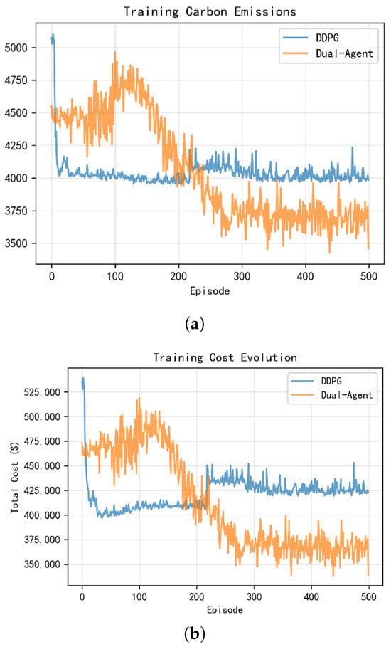
Figure 7. Training evolution of key metrics for DDPG and the proposed Dual-Agent framework: (a) total carbon emissions and (b) total operating cost versus episode.

7. Conclusions

A dual-agent deep reinforcement learning framework is proposed for low-carbon, source–load coordinated dispatch in wind-integrated distribution networks. The framework integrates the PPO algorithm, which optimizes economic performance by accounting for generation costs, curtailment penalties, and stepped carbon pricing, and the SAC algorithm, which focuses on carbon reduction and renewable accommodation. The final control action is derived via $\alpha$–$\beta$ weighted fusion, with policy-level constraints guiding DR to wind-rich periods and regulating its magnitude, while thermal power generation is coordinated with wind output under ramp-rate and minimum-output limits. Case studies on the PJM-5 test system show that, compared with a DDPG-based baseline, the proposed framework reduces operating costs by 16.8%, carbon emissions by 11.3%, and wind curtailment by 15.2% while increasing the share of renewable generation. These results underscore the framework’s application potential in high-renewable-penetration microgrids, integrated energy systems, and feeder-level dispatch, especially under carbon pricing and demand response conditions.

References

- International Renewable Energy Agency (IRENA). World Energy Transitions Outlook 2024: 1.5 °C Pathway; International Renewable Energy Agency: Abu Dhabi, United Arab Emirates, 2024; Available online: https://www.irena.org/publications (accessed on 10 December 2025).
- Arévalo, P.; Ochoa-Correa, D.; Villa-Ávila, E. Optimizing Microgrid Operation: Integration of Emerging Technologies and Artificial Intelligence for Energy Efficiency. Electronics 2024, 13, 3754. [Google Scholar] [CrossRef]
- Liu, Z.; Gao, Y.; Li, T.; Zhu, R.; Kong, D.; Guo, H. Considering the tiered low-carbon optimal dispatching of multi-integrated energy microgrid with P2G-CCS. Energies 2024, 17, 3414. [Google Scholar] [CrossRef]
- Ouyang, T.; Li, Y.; Xie, S.; Wang, C.; Mo, C. Low-carbon economic dispatch strategy for integrated power system based on the substitution effect of carbon tax and carbon trading. Energy 2024, 294, 130960. [Google Scholar] [CrossRef]
- Wei, Y.; Wang, X.; Zheng, J.; Ding, Y.; He, J.; Han, J. The carbon reduction effects of stepped carbon emissions trading and hybrid renewable energy systems. Environ. Sci. Pollut. Res. 2023, 30, 2184–2198. [Google Scholar] [CrossRef]
- Ji, X.; Li, M.; Li, M.; Han, H. Low-carbon dispatch of multi-regional integrated energy systems considering integrated demand side response. Front. Energy Res. 2024, 12, 1361306. [Google Scholar] [CrossRef]
- Sohrabi Tabar, V.; Abbasi, V. Energy management in microgrid with considering high penetration of renewable resources and surplus power generation problem. Energy 2019, 189, 116264. [Google Scholar] [CrossRef]
- Chen, S.; Liu, J.; Cui, Z.; Chen, Z.; Wang, H.; Xiao, W. A Deep Reinforcement Learning Approach for Microgrid Energy Transmission Dispatching. Appl. Sci. 2024, 14, 3682. [Google Scholar] [CrossRef]
- Mu, C.; Shi, Y.; Xu, N.; Wang, X.; Tang, Z.; Jia, H.; Geng, H. Multi-objective interval optimization dispatch of microgrid via deep reinforcement learning. IEEE Trans. Smart Grid 2023, 14, 1790–1799. [Google Scholar] [CrossRef]
- Alabi, T.M.; Lawrence, N.P.; Lu, L.; Yang, Z.; Gopaluni, R.B. Automated deep reinforcement learning for real-time scheduling strategy of multi-energy system integrated with post-carbon and direct-air carbon capture systems. Appl. Energy 2023, 333, 120633. [Google Scholar] [CrossRef]
- Huang, S.; Li, P.; Yang, M.; Gao, Y.; Yun, J.; Zhang, C. A control strategy based on deep reinforcement learning under the combined wind-solar storage system. IEEE Trans. Ind. Appl. 2021, 57, 6547–6558. [Google Scholar] [CrossRef]
- Bian, J.; Wang, Y.; Dang, Z.; Xiang, T.; Gan, Z.; Yang, T. Low-carbon dispatch method for active distribution network based on carbon emission flow theory. Energies 2024, 17, 5610. [Google Scholar] [CrossRef]
- Cao, D.; Hu, W.; Xu, X.; Wu, Q.; Huang, Q.; Chen, Z.; Blaabjerg, F. Deep reinforcement learning based approach for optimal power flow of distribution networks embedded with renewable energy and storage devices. J. Mod. Power Syst. Clean Energy 2021, 9, 1101–1110. [Google Scholar] [CrossRef]
- Long, Y.; Li, Y.; Wang, Y.; Cao, Y.; Jiang, L.; Zhou, Y.; Deng, Y.; Nakanishi, Y. Low-carbon economic dispatch considering integrated demand response and multistep carbon trading for multi-energy microgrid. Sci. Rep. 2022, 12, 6218. [Google Scholar] [CrossRef] [PubMed]
- Li, J.F.; He, X.T.; Li, W.D.; Zhang, M.; Wu, J. Low-carbon optimal learning scheduling of the power system based on carbon capture system and carbon emission flow theory. Electr. Power Syst. Res. 2023, 218, 109215. [Google Scholar] [CrossRef]
- Wu, X.; Chen, Q.; Zheng, W.; Xie, J.; Xie, D.; Chen, H.; Yu, X.; Yang, C. Low-Carbon Dispatch Method Considering Node Carbon Emission Controlling Based on Carbon Emission Flow Theory. Energies 2025, 18, 5050. [Google Scholar] [CrossRef]
- Liu, J.; Zhao, H.; Wang, S.; Liu, G.; Zhao, J.; Dong, Z.Y. Real-time emission and cost estimation based on unit-level dynamic carbon emission factor. Energy Convers. Econ. 2023, 4, 47–60. [Google Scholar] [CrossRef]
- Liu, W.C.; Mao, Z.Z. Microgrid economic dispatch using information-enhanced deep reinforcement learning with consideration of control periods. Electr. Power Syst. Res. 2025, 239, 111244. [Google Scholar] [CrossRef]
- Gu, Y.; Cheng, Y.; Chen, C.L.P.; Wang, X. Proximal policy optimization with policy feedback. IEEE Trans. Syst. Man Cybern. Syst. 2021, 52, 4600–4610. [Google Scholar] [CrossRef]
- Zhao, L.; Li, F.; Zhou, Y.; Fan, W. Soft Actor-Critic-based grid dispatching with distributed training. In Proceedings of the 2023 International Conference on Mobile Internet, Cloud Computing and Information Security (MICCIS), Nanjing, China, 24–26 November 2023; pp. 1–6. [Google Scholar] [CrossRef]
- Li, G.Q.; Zhang, R.F.; Jiang, T.; Chen, H.; Bai, L.; Cui, H.; Li, X. Optimal dispatch strategy for integrated energy systems with CCHP and wind power. Appl. Energy 2017, 192, 408–419. [Google Scholar] [CrossRef]
- Silver, D.; Lever, G.; Heess, N.; Degris, T.; Wierstra, D.; Riedmiller, M. Deterministic policy gradient algorithms. In Proceedings of the International Conference on Machine Learning (ICML), Beijing, China, 21–26 June 2014; pp. 387–395. [Google Scholar]
Disclaimer/Publisher’s Note: The statements, opinions and data contained in all publications are solely those of the individual author(s) and contributor(s) and not of MDPI and/or the editor(s). MDPI and/or the editor(s) disclaim responsibility for any injury to people or property resulting from any ideas, methods, instructions or products referred to in the content. |
© 2026 by the authors. Licensee MDPI, Basel, Switzerland. This article is an open access article distributed under the terms and conditions of the Creative Commons Attribution (CC BY) license.